A Trip Generation Model for a Petrol Station with a Convenience Store and a Fast-Food Restaurant

Abstract

A trip generation manual and database are important for transportation planners and engineers to forecast new trip generation for any new development. Nowadays, many petrol stations have fast-food restaurant outlets. However, this land use category has yet to be included in the Malaysian Trip Generation Manual. Therefore, this study attempted to develop a new trip generation model for the new category of “petrol station with convenience store and fast-food restaurant”. Significant factors influencing the trip generation were also determined. Manual vehicle counts at the selected sites were conducted for 3 h during morning, afternoon and evening peak hours. Regression analysis was used in this study to develop the model. A simple trip generation model based on the independent variable number of restaurant seats showed a greater value for the coefficient of determination, R², compared with the independent variables gross floor area in thousand square feet and number of pumps. The multivariable trip generation model using three independent variables generated the highest R² among all of the models but was still below a satisfactory level. Further study is needed to improve the model for this new land use category. We must ensure more accuracy in trip generation estimation for future planning and development.

1. Introduction

Land use and transportation are interdependent; therefore, it is very important to understand the relationship between land use and transportation in order to plan for a sustainable and safe transportation system [1]. When land is developed or expanded, engineers and transport planners need to predict the vehicle trips to be generated with regard to the developments, bringing additional trips to the existing road network. The extra demands for transport have resulted in some existing roads losing their capacity to accommodate traffic, resulting in traffic congestion, traffic jams and severe accidents [2]. Therefore, an accurate prediction of trips is important to investigate the impact of the development on the performance of the existing road and junctions. From this estimate, a developer has to provide sufficient road facilities to accommodate the additional trips. As a result, even with a further increase in traffic volume on the road network, the sustainability of the road network can be maintained, which will benefit current and future road users.

A trip generation manual or database is used by transportation and town planners to estimate the number of trips generated by a specific new development or an expansion of an existing development. A petrol station, also known as a filling station or gas station, is a place that sells fuel for road vehicles [3]. Nowadays, petrol stations offer a variety of goods and services in order to attract more customers and to increase business opportunities. Many big oil and gas companies around the world have established partnerships with fast-food companies, such as Casey’s and TravelCenters of America partnering with A&W [4], Sinopec Corp and China National Petroleum Corporation (CNPC) partnering with Kentucky Fried Chicken (KFC) [5] and, in Malaysia, Petronas also partnering with KFC [6].

The Malaysian Trip Generation Manual (MTGM) consists of 160 categories of land use, including petrol stations with or without convenience stores [7]. Petrol stations in this category are located along main roads for motorists to easily refuel their vehicles. Most of them provide extra services, such as convenience stores, minor motor vehicle repairs or a servicing and car wash center. Thus, with changes in the typical profile of petrol stations in Malaysia, the category of petrol station in the manual is no longer reliable. Therefore, this study focuses on a model made to predict trips for petrol stations with fast-food restaurants.

2. Background

Trip generation is the first step in the conventional four-step transport forecasting process and is widely used for forecasting travel demands [8]. Thus, it is crucial to perform it right from the beginning to ensure the next steps—trip distribution, mode choice and route assignment—are properly conducted and that the end results are correct. Furthermore, trip generation study is important for in-depth traffic analyses, decongestion strategies [9] and traffic impact assessments [10].

Trip generation estimates the total number of trips produced from a zone and attracted to a zone [11]. In addition to each unique land use characteristic, many studies found other demographic and socioeconomic factors also influence trip generation, such as age, education level, occupation, license ownership, vehicle ownership, household income, household size and population [12,13,14]. Household trip questionnaires are used to collect this information; however, they are very expensive to conduct, and many cities cannot afford to carry out surveys as often as would be useful [15,16]. Therefore, a model that requires less data is more appropriate [17]. It is impractical to use a trip generation model with demographic and socioeconomic variables for a traffic impact study if there was a lack of suitable data at the early stage of development. Therefore, the study focuses on land use characteristics prevalent during this stage.

A trip generation model is built on the relationships between trip generation and independent variables representing land uses in order to correctly forecast future trips when the variables are known [18]. A suitable independent variable based on land use characteristics should be investigated when determining the trip generation model. The Institute of Transportation Engineers’ (ITE) Trip Generation Manual currently has five land use categories related to gas stations with or without convenience stores. One of them is a truck stop that provides dedicated diesel pumps, others are differentiated by the gross floor area of the convenience store and the number of pumps. The independent variables for the gas station land use category in the ITE manual are thousand square feet of gross floor area (GFA) of the convenience store, AM/PM peak hour traffic on the adjacent street, the number of employees and the number of pumps [19]. Studies on trip generation for petrol stations mostly use GFA and the number of pumps as independent variables in developing a trip generation model, such as studies conducted in Florida [20], Nigeria (along Lasu-Isheri road corridor) [21] and Maryland and New Jersey [22]. However, Utainarumola and Ampawasuvanb [23] found that other significant variables can affect the traffic into and out of the fuel station located on an arterial road in Thailand, such as the traffic volume on the arterial road, the size of the fuel station, the number of pumps and the density of fuel stations located on routes toward food center areas and convenience store areas. Cunningham et al. [24] recommended the trip generation equation for fueling centers should incorporate average daily traffic (ADT) and whether the station is a hybrid station, whereby the station does not have a fast-food outlet but a customer can order certain food, such as sandwiches and soft drinks or coffee, and there is a drive through facility.

Regression models are regularly used in trip generation analysis [12,13,14,25,26]. The cross-classification method is another technique used [27,28]; however, the main drawback is that it is too costly due to its sample size requirements and lack of goodness of fit measures [29]. Besides, regression models are accommodative to multiple independent variables [30]. Multiple stepwise regression was used in Shi and Zhu’s study [8] to calculate the commuting trip production and attraction rates for all residential land and each subdivided housing type during morning peak hours. Multiple stepwise regression may be used to screen and remove variables that may cause multicollinearity. Logistic or logit regression analysis may overcome several constraints of linear regression analysis, which assumes independent variable linearity with dependent variables, and category analysis, which requires a large sample size. It can be used to determine a decision boundary for a binary classification problem. In Hanoi, Vietnam, Nguyen et al. [31] used a logit model for destination choice and an ordered probit model for trip generation with socio-demographic, mobility and accessibility and built environment factors. Gim [32] used multinomial logistic regression models to analyze the relationship between land use and destination choice separately for weekday and weekend travel with land use variables, trip characteristics and individual and household socio-demographics. However, these studies focused on personal trips and trip purpose, which could not be addressed in this study.

Land use forecasting can include single-variable and multivariable regression analysis [33]. A trip generation linear regression model can be developed based on the assumption that there are linear relationships between dependent and independent variables. Another assumption is that the calculation of the dependent variable’s value will be better with more independent variables [34]. Initially, the trip generation model developed by the ITE used simple regression analysis [13]. Nevertheless, in its 10th edition, the ITE introduced a multivariable trip generation equation for three land use categories. Two of them are related to petrol stations, namely the gasoline/service station with convenience market and super convenience market/gas station [35]. Cunningham et al. [24] found that multivariable equations are able to give more accuracy in trip estimation for modern fueling centers compared to single-variable methods. The multiple regression models developed had reasonable correlations and provided superior predictions in comparison to the single-variable models. A study in New Jersey found that neither the size of the convenience store nor the number of pumps alone are sufficient as a trip generation variable when single-variable regression analysis is performed. Therefore, future trip generation analysis should consider multivariable regression analysis of these factors [22].

The Trip Generation Manual published by the ITE is the most comprehensive document on trip generation [36]. The manual provides trip generation rates for numerous types of land use. The ITE procedure is to forecast the inbound and outbound traffic for land use during a specific period based on the given rate. However, the ITE manual was developed based on travel behavior in the United States and Canada. Thus, the model may not be suitable for other countries. Several countries have conducted studies to develop local trip generation rates based on the characteristics observed in their communities; some even have their own trip generation databases and manuals. For example, TRICS for the UK and Ireland [37]; the Guide to Traffic Generating Developments by Australia Road and Maritime Services [38]; the Trips Database Bureau (TDB), which consists of data on parking and traffic surveys in New Zealand and Australia [39]; the South African Trip Data Manual; and the Trip Generation and Parking Rates Manual Emirate of Abu Dhabi [10]. In Malaysia, a total of 1178 sites from various land use types and locations throughout Malaysia were surveyed since 1995 to publish the current 2010 MTGM [40].

In MTGM, the petrol station trip generation model used GFA and number of pumps as independent variables. Unfortunately, from the statistical analysis, no linear relationship between number of trips and GFA or between number of trips and number of pumps was shown [41]. Thus, the model is not suitable to use for prediction. Motivated by this reason and the changes in petrol stations’ features in Malaysia, this study had the objective of developing a novel and more accurate trip generation model for the new category of petrol station with a convenience store and a fast-food restaurant. Firstly, the significant factors influencing the trip were determined. Subsequently, a mathematical model describing the relationships between trips generated by the new petrol station category and its characteristics were derived using statistical analysis. In addition, this study tested the hypotheses that the use of our model for petrol stations in MTGM would result in inaccurate predictive trip generation for a petrol station with a fast-food restaurant and that a multivariable model would be better for predicting trips to a petrol station with a fast-food restaurant compared to a simple model. The model developed must be included in MTGM under a new subcategory, ensuring the forecasted rate for this category is accurate and reliable.

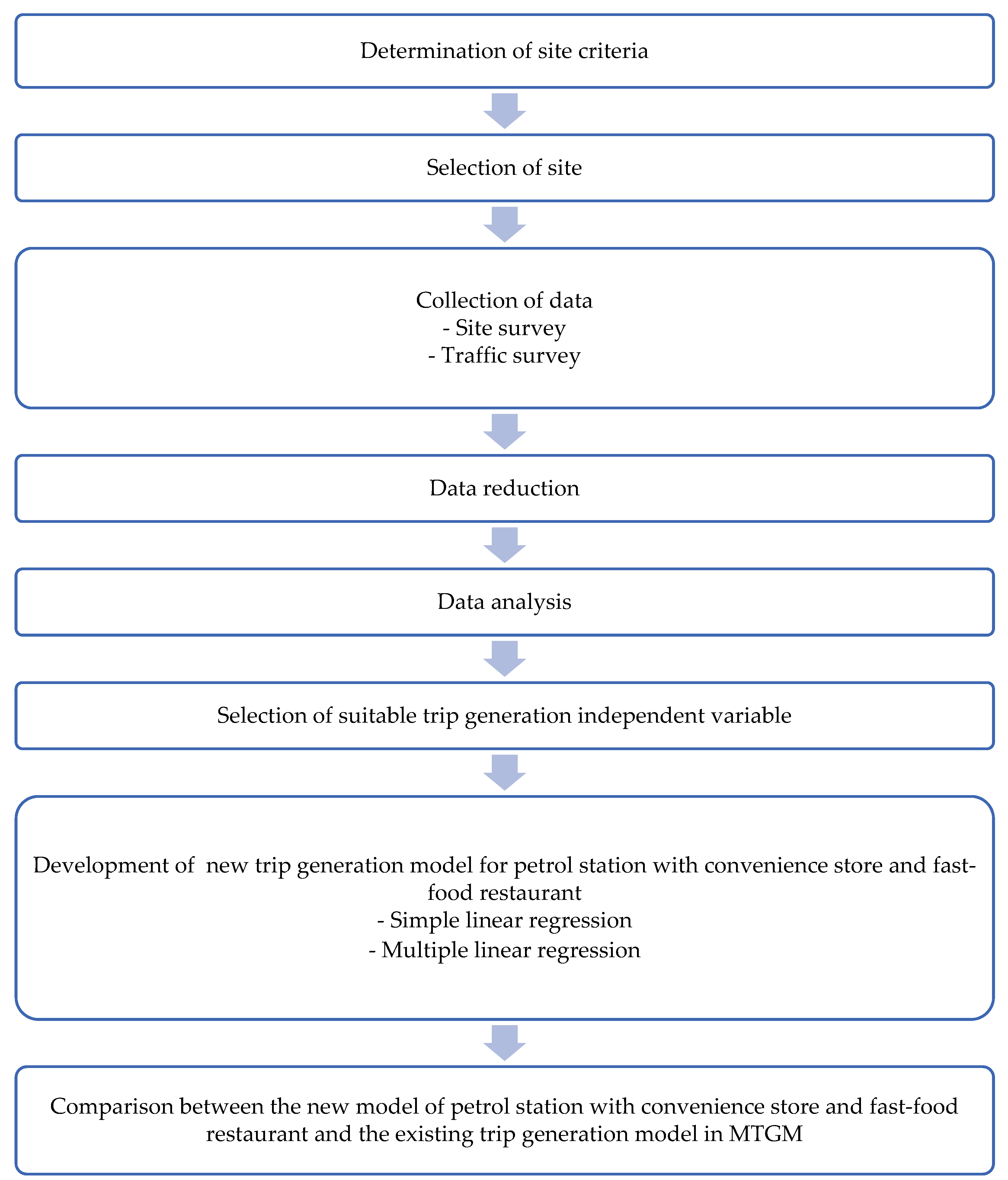
3. Research Methodology

Figure 1 summarizes the methodology applied to achieve the objectives of this study. The methodology used is similar to that of the Malaysian Trip Generation Study Phase IV [40]. The Malaysian Trip Generation Study Phase IV methodology was developed based on the ITE method. Even though this method is unable to account for multimodal behavior in urban contexts [10,42], this method has been widely used due to its simplicity and the availability of data. The cost is moderate because there is no need for special equipment or software. In this study, additional site selection criteria were added. The petrol station selected had to share the same access road and parking with the attached fast-food restaurant with a drive-through facility. In terms of analysis, this study also looked at multiple linear regression, not only using single linear regression as in the MTGM. Other criteria included that the site should be mature (at least 2 years old) and that there is no major activity within the vicinity, such as on site or nearby construction, which might affect trip patterns. In addition, site information had to be available, such as floor area, number of pumps and number of restaurant seats. Last but not least, approval from the station owners for the study to be conducted at their station was needed. Site reconnaissance was conducted in Klang Valley and in Penang state to identify petrol stations with the criteria that were predetermined in the early stage of the study. Klang Valley and Penang were selected because of their high-density populations [43]. There is no established statistical approach to choosing the number of sites required to provide statistically significant trip generating estimates. However, the ITE suggests surveying at least three (preferably five) sites [44], though a larger number of studies depend on time and financial restrictions. Furthermore, in trip generating studies, particularly on newly established land use sub-categories (such as “petrol station with a convenience store and a fast-food restaurant”), it is usual practice to collect data at just several sites that satisfy the required site selection criteria to study the trend before a proper trip generation estimation model can be established. Additionally, because this land use category is still in its early stages of development, only a few petrol stations were available for data collection and some of them were inaccessible due to the owners’ unwillingness to participate. Therefore, only ten petrol stations in Klang Valley and in Penang state were selected for observation in this study. Data collection was performed via site survey and traffic survey.

3.1. Site Survey

Table 1. Site details.

Site		GFA	Pump	Seat	Operational Hours		ATM Services	No. of Entrance/Exit Points 1 and Their Location
No.	Details				Petrol Station	Restaurant
1	Petronas/McDonald’s/Subway	10.82	9	140	18 (0600–0000)	24	Yes	1C–Federal Road 1C–Local Street
2	Petronas/ Kentucky Fried Chicken	10.89	16	112	24	24	Yes	1E–Expressway 1T–Expressway 1C–Local Street
3	Petronas/McDonald’s	8.80	16	128	24	24	Yes	1E–Federal Road 2T–Federal Road
4	Petronas/Burger King	9.20	13	92	24	15 (0800–2300)	Yes	1E–Federal Road 1T–Federal Road 1C–Local Street
5	Petronas/ Starbucks/Dunkin’ Donuts	10.42	14	138	24	20 ½ (0630–0300)	Yes	1E–Federal Road 1T–Federal Road
6	Petronas/ Kentucky Fried Chicken	7.41	12	112	24	12 (1000–2200)	No	1E–Federal Road 2T–Federal Road
7	Shell/ McDonald’s	5.77	19	102	24	24	Yes	1E–Federal Road 1T–Federal Road
8	Shell/ McDonald’s/ 7-Eleven	9.17	20	71	24	24	Yes	1E–Federal Road 1T–Federal Road
9	Shell/ McDonald’s/ 7-Eleven	12.83	16	124	18 (0600–0000)	24	Yes	1E–Federal Road 1T–Federal Road
10	BHPetrol/McDonald’s	9.94	13	167	24	24	Yes	1E–Federal Road 1C–Local Street

¹ C—combined entrance and exit, E—entrance only, T—exit only.

shows the details of each site gathered from the station’s owner or staff and from on-site observation. All stations except site number 6 had an automatic teller machine (ATM). Total GFA, number of pumps (pump) and number of restaurant seats (seat) were identified as independent variables for the model. GFA was between 5.77 and 12.83 thousand square feet (tsf). Site 9 had the largest GFA, 12.83 tsf. Site 7 had the smallest floor area, 5.77 tsf, but the second largest number of pumps—19 pumps. The fast-food restaurant at site 8 had the smallest number of seats, 71, whereas site 10 had the largest number of seats, 167. All stations operate 24 h a day, except site 1 and site 9, which operate from 6 a.m. to 12 a.m. only. The fast-food restaurant at sites 4, 5 and 6 do not operate 24 h a day, even though the petrol stations do. All sites except site 2 are located beside federal roads. Site 2 is located at the access road beside an expressway. It has one entrance and exit point from the expressway and another access point from a local street. Sites 1, 4 and 10 also have access roads connected to local streets.

3.2. Traffic Count

Each manual vehicle counting survey was conducted for nine hours per day, divided into 3-h sessions for a morning period (0645–0945), an afternoon period (1130–1430) and an evening period (1645–1945) on a typical working day, Tuesday, Wednesday or Thursday. This was to identify the peak period (hour) that recorded the highest total of inbound and outbound trips at each site in the morning, afternoon and evening. On-site equipment included a pen, a survey form and a video camera for data verification later. Enumerators were stationed at each access point to record numbers of vehicles entering and exiting the station, including the drive-through users in a 15 min interval based on types of vehicles. The categories of vehicle in this study are the same as those in the MTGM, as shown in

Table 2. Vehicle types and passenger car unit (pcu) factor used in the MTGM.

Vehicle Type	pcu
Car	1.00
Taxi	1.00
Small van	1.00
Large van, light lorry (2 axles)	1.75
Heavy lorry (>2 axles)	2.25
Bus	2.25
Motorcycle	0.33

. Through traffic (rat-running) that used the site as a shortcut was also identified; it was excluded from the analysis because it does not represent purposeful trips to the area.

4. Results and Discussion

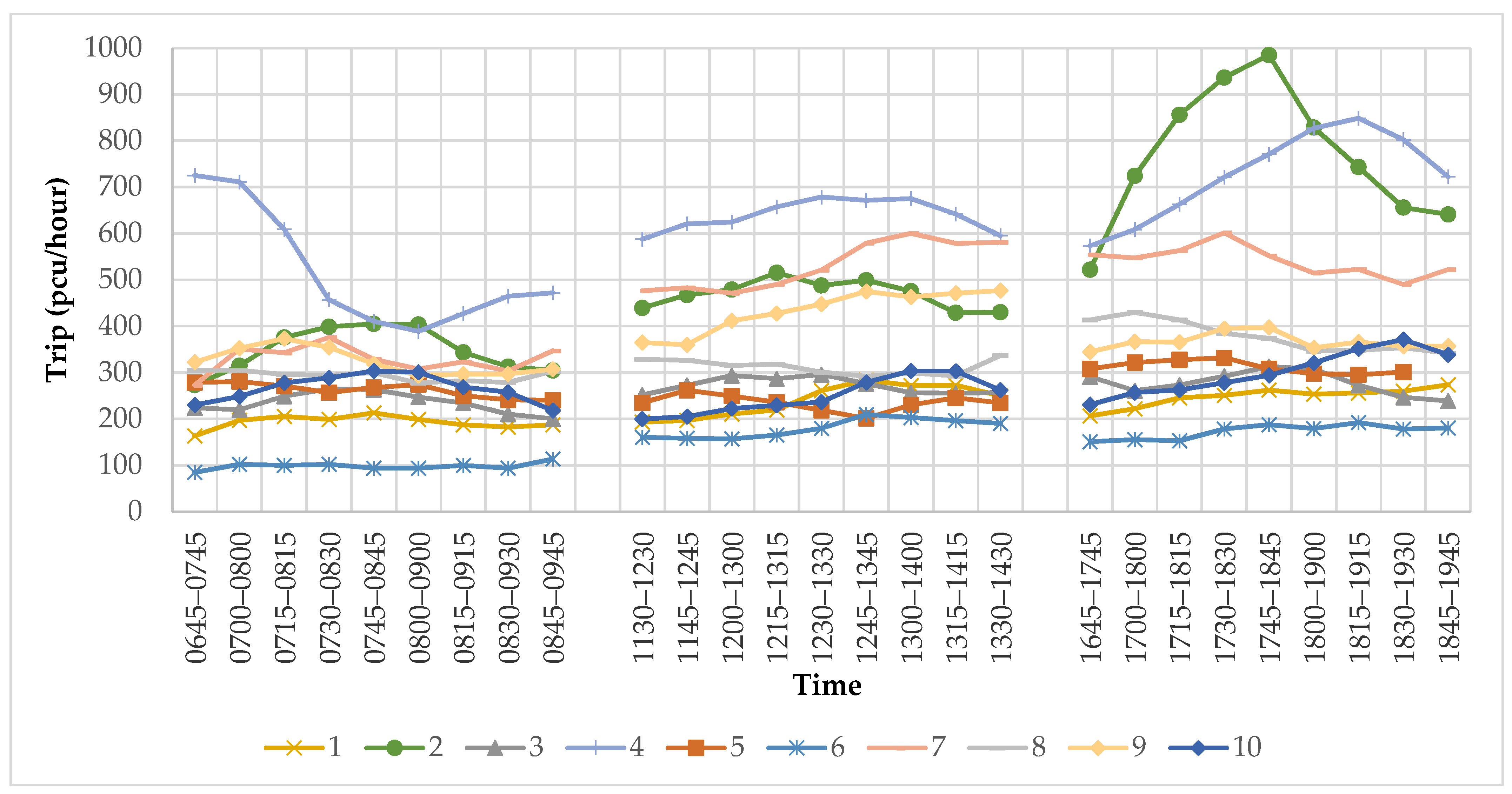
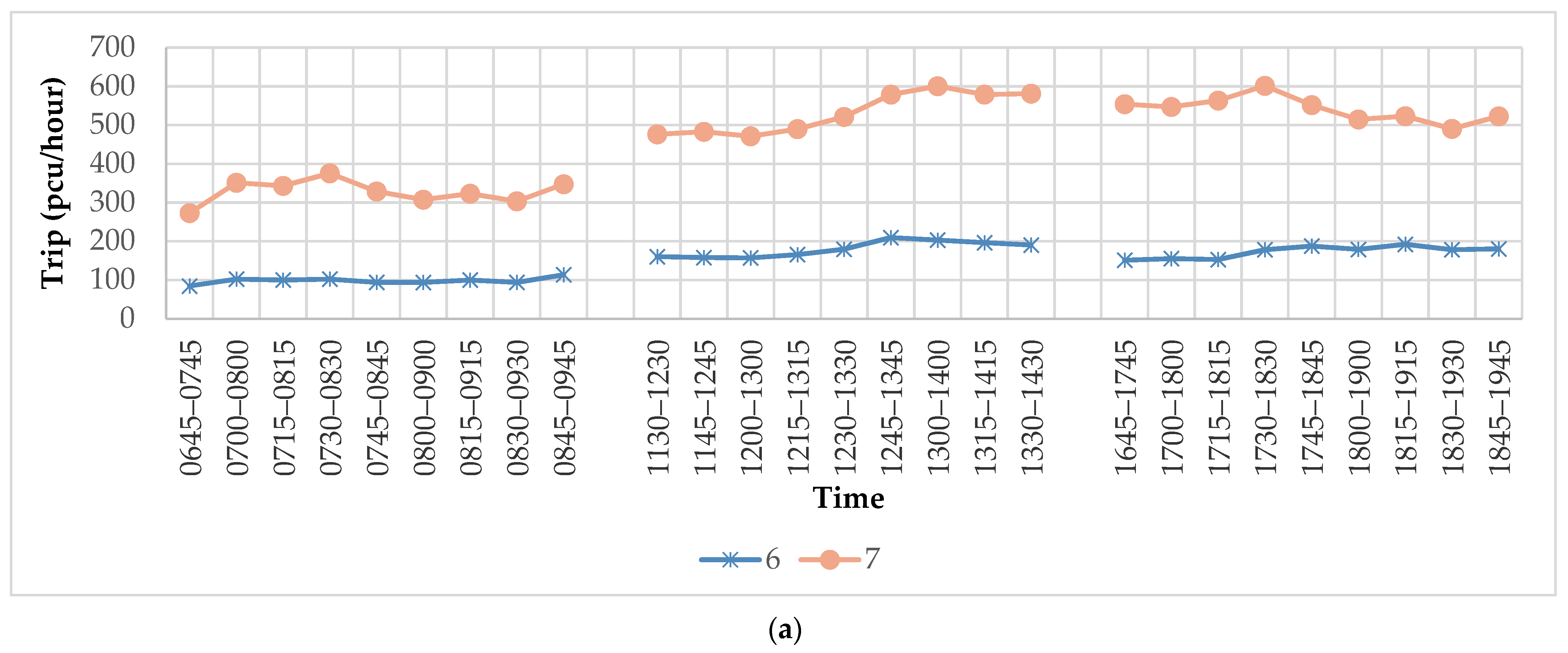
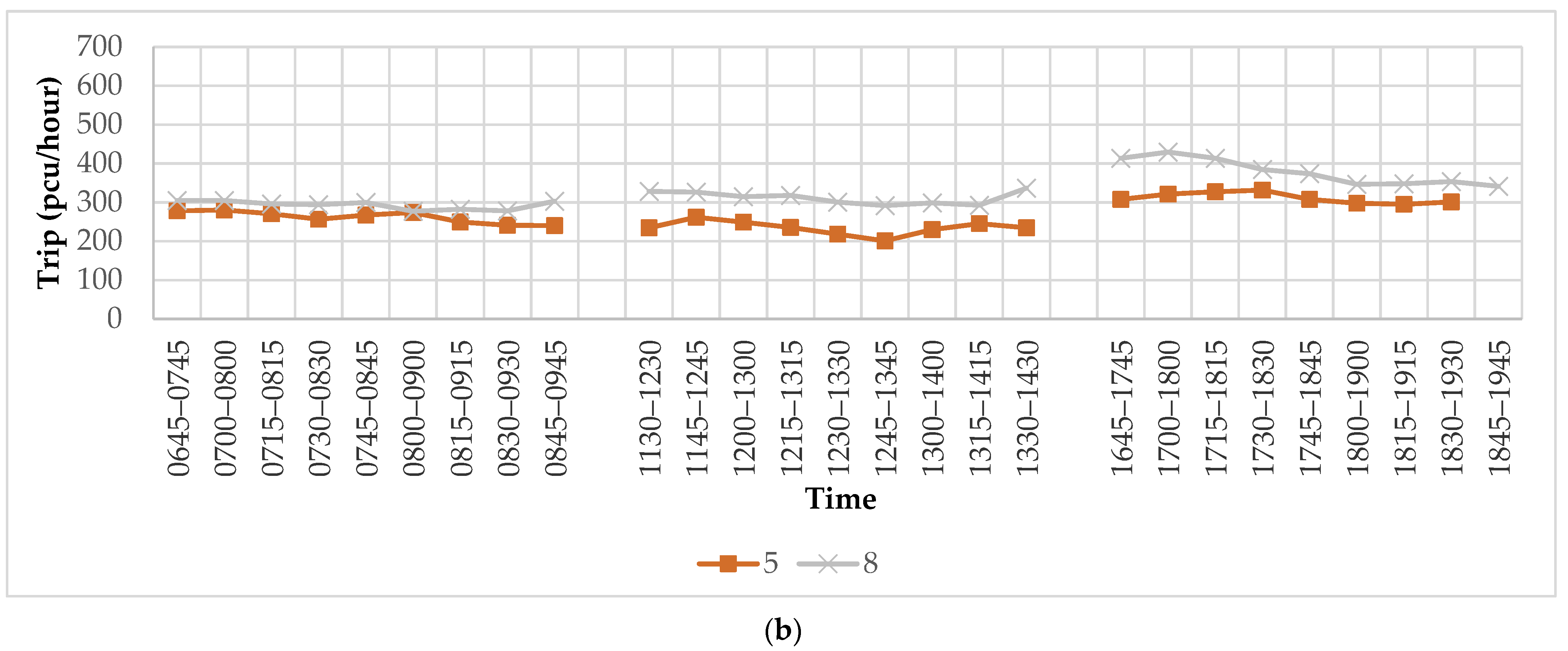
4.1. Peak Hour Traffic Volume

Table 3. Peak hour trip types and vehicle types.

Site No.	Peak	Time	Trip (pcu/h)	Trip (%)		Trip (%)	Vehicle Type (%)
				Inbound	Outbound	Drive-Through	Car/ Taxi/ Small Van	Large Van/ Light Lorry	Heavy Lorry	Bus	Motorcycle
1	Morning peak	0745–0845	213	53	47	4	64	2	0	0	34
	Afternoon peak	1245–1345	284	53	47	3	57	5	0	1	37
	Evening peak	1845–1945	273	56	44	6	64	3	0	0	34
2	Morning peak	0745–0845	405	52	48	0	66	3	0	1	30
	Afternoon peak	1215–1315	516	59	41	4	78	3	1	0	19
	Evening peak	1745–1845	985	53	47	3	77	1	0	0	21
3	Morning peak	0730–0830	265	47	53	10	69	1	1	0	29
	Afternoon peak	1230–1330	296	47	53	9	70	19	1	0	10
	Evening peak	1745–1845	313	43	57	13	73	7	1	0	20
4	Morning peak	0645–0745	725	52	48	0	69	2	0	0	29
	Afternoon peak	1230–1330	679	38	62	2	75	3	0	0	22
	Evening peak	1815–1915	849	24	76	2	70	1	0	0	29
5	Morning peak	0700–0800	281	50	50	2	83	9	0	0	7
	Afternoon peak	1145–1245	262	52	48	4	84	6	1	0	8
	Evening peak	1730–1830	332	43	57	6	84	3	1	0	12
6	Morning peak	0845–0945	113	54	46	2	65	5	0	0	30
	Afternoon peak	1245–1345	210	44	56	13	75	5	1	0	20
	Evening peak	1815–1915	192	49	51	7	56	0	0	0	44
7	Morning peak	0730–0830	376	53	47	6	66	3	0	0	31
	Afternoon peak	1300–1400	600	58	42	11	82	4	0	0	13
	Evening peak	1730–1830	601	53	47	5	66	1	0	0	33
8	Morning peak	0700–0800	305	60	40	8	80	5	0	1	15
	Afternoon peak	1330–1430	337	62	38	7	83	5	0	0	12
	Evening peak	1700–1800	430	59	41	8	76	5	1	0	18
9	Morning peak	0715–0815	373	58	42	6	60	2	0	0	38
	Afternoon peak	1330–1430	477	65	35	14	79	2	0	0	19
	Evening peak	1745–1845	397	60	40	15	73	1	0	0	26
10	Morning peak	0745–0845	303	54	46	7	76	2	2	0	20
	Afternoon peak	1300–1400	304	56	44	11	80	5	0	0	15
	Evening peak	1830–1930	371	60	40	13	84	1	0	0	14
Average	Morning peak			53	47	5	70	3	0	0	26
	Afternoon peak			53	47	8	76	6	0	0	18
	Evening peak			50	50	8	72	2	0	0	25

shows the trips per hour and the composition of vehicle types during peak hours. Vehicle count data were changed to pcu units (Table 2) for analysis purposes. Site 4 recorded the highest trip count during the morning peak, with 725 pcu/h, and during the afternoon peak, with 679 pcu/h. For evening peak hour, site 2 recorded the highest number of trips, with 985 pcu/h. Site 6 recorded the lowest number of trips for all peak hour periods, with 113 pcu/h (morning), 210 pcu/h (afternoon) and 192 pcu/h (evening). All sites recorded the most visitation during their evening peak hours, except for sites 1, 6 and 9. At those sites, the most traffic was recorded during the afternoon peak.

Average percentages of inbound and outbound trips (in the given 3-h intervals) accounted for by morning and afternoon peak hours were 53% and 47%, respectively, and 50% was accounted for by the evening peak. Drive-through trips were less than 10% of total trips for all sites except at site 3 (morning and evening), sites 6 and 7 (afternoon) and sites 9 and 10 (afternoon and evening). All sites recorded the least drive-through trips, proportionally, during the morning peak period.

In terms of types of vehicles, the car/taxi/small van category made up the highest percentage for all peak hours, with more than 70%, followed by motorcycles. Site 5 recorded the lowest percentages of motorcycle trips, with 7%, 8% and 12% (morning, afternoon and evening).

Figure 2 shows the traffic volume fluctuations based on data collected at each site. Site 4 had the highest trips per hour during both morning (except between 0800 and 0900) and afternoon periods. This is because of its location next to a hypermarket and its distance from other stations is quite far. On the other hand, site 2 had the highest number of trips per hour for the evening period, from 1745 to 1845, with 985 pcu/h. In contrast, site 6 had the lowest number of trips per hour; the largest recorded value was only 210 pcu/h, from 1245 to 1345. Sites 2 and 4 have access from local roads, but not site 6. The access points to site 6 are from Federal Road, which is quite far from the housing and business area and might be the reason for the lowest trip numbers. In addition, competition with a station next door that is very close might be the other reason. Semih and Seyhan found that amongst the criteria that play key roles in selecting a gas station site, there is access to the station from both directions; location on a local or state road; other competitors in the area; and factors related to the neighborhood, such as other close-by businesses affecting the traffic [45].

Sites 6 and 7 are located next to each other, similarly to sites 5 and 8. However, the difference in traffic volume recorded between sites 6 and 7 is more obvious than that between sites 5 and 8. This is clearly depicted in Figure 3a,b. The big gap in traffic volume between sites 6 and 7 may be contributed to by the station’s brand and the fast-food restaurant’s brand. A survey finding showed that customers select petrol stations based on location, quality of service, station size and brand image [46]. As for fast-food restaurants, a survey conducted among undergraduates shows that the most preferred brand is McDonald’s, followed by KFC, Pizza Hut, Wing Zone and Domino’s Pizza [47]. Three main factors that influence the choice of fast-food restaurants are price, customer service and restaurant environment [46,47]. Brand reputation is the main factor for customers in Bangladesh in choosing their fast-food restaurants. Other reasons are proximity and accessibility [48]. Thus, in the case of two fast-food restaurants located beside each other, brand reputation is the main consideration.

4.2. Trip Generation Variable

Based on studies discussed in Section 2, the number of pumps and GFA are always considered as independent variables for a petrol station trip generation model. Al-Madadhah and Imam [49] found that the number of seats is the best predictor for a fast-food restaurant. Hence, in this study, the dependent variable was the total number of inbound and outbound trips entering and leaving a petrol station, and the independent variables were number of pumps, GFA and number of restaurant seats. GFA is the total floor area of a building, including its corridor, calculated in thousand square feet. Number of pumps refers to the total number of filling points at each station at any one time, and the number of seats does account for some seats having room for multiple people.

4.3. Trip Generation Model

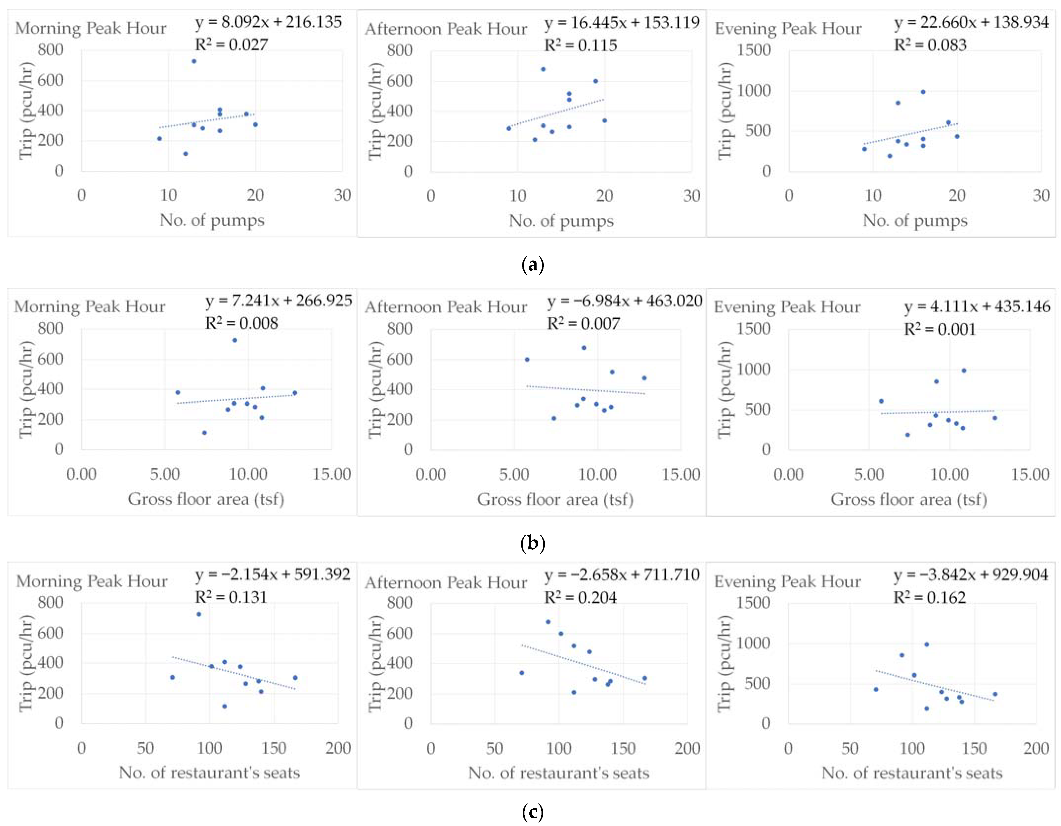
4.3.1. Simple Linear Regression

Regression is the statistical technique of modeling the relationship between variables. It can be used to predict outcomes for the independent and dependent variables in data. When there is only one independent variable in the linear regression model, the model is called a simple linear regression model. The coefficient of determination, R², represents the percent of variation in the dependent variable that can be explained by variation in the independent variable using the regression line [50]. The R² always lies between 0 and 1. A higher R² indicates a better model fit. Figure 4 shows the simple linear regression graph of the trip generation model using the number of pumps, GFA and the number of restaurant seats for three peak hour periods as independent variables. The trip generation model developed for all the independent variables shows a low R² value of less than 0.21. Therefore, more than 79% of the variation in trip cannot be explained by the variation in number of pumps, GFA and number of restaurant seats by the regression line. The MTGM recommends using a trip generation equation if the R² value is at least 0.50 [7], whereas the ITE recommends at least 0.75 [46]. Thus, it is not recommendable to use this regression equation to predict trip generation. Nevertheless, the trip number showed positive relationships with number of pumps and GFA (except for the afternoon peak model) but showed a negative linear relationship with the number of restaurant seats. Moreover, Ahmed [51] could not establish a clear relationship between trips and number of seats and found that the number of seats could not reliably predict trips to fast-food restaurants in Malaysia.

The Shapiro–Wilk test is used to examine the normality of data with a sample size less than 50 [52]. If p < 0.05, it rejects the null hypothesis of a normal population in a distribution. All models retained the null hypothesis of population normality because p > 0.05 except for the number of pumps variable in the evening peak model. The Shapiro–Wilk test showed a significant departure from normality for that model, W(10) = 0.770, p = 0.006, which indicates the model was biased. Any outlier causing the model to fail in the normality test needed to be identified. Standardized residuals were computed to identify the existence of outliers in the model. A large, standardized residual of (d > 3) indicates an outlier [53]. All data points indicate d < 3, which means there were no potentially high-influence points.

However, due to low sample sizes, this finding should not be interpreted as a conclusive finding for this study but rather as a basis for further investigation. Nevertheless, in order to improve on the predictive capability of the regression model, a further attempt to add more variables in the regression model was conducted through multiple linear regression analysis.

4.3.2. Multiple Linear Regression

Multiple regression is an extension of simple linear regression. It is a model for predicting the value of one dependent variable based on two or more independent variables. The regression analysis results in

Table 4. Results of regression analysis on number of pumps, total GFA and number of restaurant seats with trip.

Model 1	Independent Variable (x)	Dependent Variable (y): Trip
		Morning			Afternoon			Evening
		β	Constant	R2	β	Constant	R2	β	Constant	R2
1	Pumps	8.092	216.135	0.027	16.445	153.119	0.115	22.660	138.934	0.083
2	GFA	7.241	266.925	0.008	−6.984	463.020	0.007	4.111	435.146	0.001
3	Seats	−2.154	591.392	0.131	−2.658	711.710	0.204	−3.842	929.904	0.162
4	Pumps	9.920	78.393	0.046	16.491	149.594	0.115	25.045	−40.852	0.096
	GFA	11.621			0.297			15.168
5	Pumps	−3.374	669.561	0.135	5.600	581.982	0.213	6.418	781.225	0.167
	Seats	−2.392			−2.263			−3.389
6	GFA	20.220	459.927	0.185	6.777	667.650	0.210	26.009	760.799	0.197
	Seats	−2.670			−2.831			−4.505
7	Pumps	−2.316	515.271	0.186	5.995	524.387	0.220	7.843	573.352	0.203
	GFA	19.960			7.451			26.891
	Seats	−2.826			−2.425			−3.974

¹ Note: Significance level, p > 0.05.

show that model 7, with independent variables number of pumps, total GFA and number of restaurant seats, produced the highest value of R² for all three peak hours, as compared to the other models. However, these R² values are considered very low: 18.6% for the morning peak hour, 22.0% for the afternoon peak hour and 20.3% for the evening peak. The model tried to explain the variation using the number of pumps, total GFA and number of restaurant seats.

The equations of multiple regression model 7 are:

Morning:   y = −2.361x₁ + 19.960x₂ − 2.826x₃ + 515.271

(1)

Afternoon:   y = 5.995x₁ + 7.451x₂ − 2.425x₃ + 524.387

(2)

Evening:    y = 7.843x₁ + 26.891x₂ − 3.974x₃ + 573.352

(3)

where y is a trip generated from the petrol station, x₁ is the number of pumps, x₂ is GFA and x₃ is the number of restaurant seats.

The variables for all models were not significant predictors of trip. Due to multicollinearity, several important variables can become statistically insignificant in multiple regression analysis [54]. The variance inflation factor (VIF) was used to determine how much the variance of the predicted regression coefficient was inflated due to the correlations among the independent variables. There is a moderate correlation between the variables if the value of VIF is 1 < VIF < 5. There was no indication of multicollinearity among the variables studied.

From the Shapiro–Wilk test, all models retained the null hypothesis of population normality because p > 0.05, except for model 4 for morning and evening peak hours. The test showed a significant departure from normality for model 4 morning peak, W(10) = 0.747, p = 0.003, and evening peak, W(10) = 0.736, p = 0.002. All data points in the models indicate d < 3, which means there were no potential high-influence points.

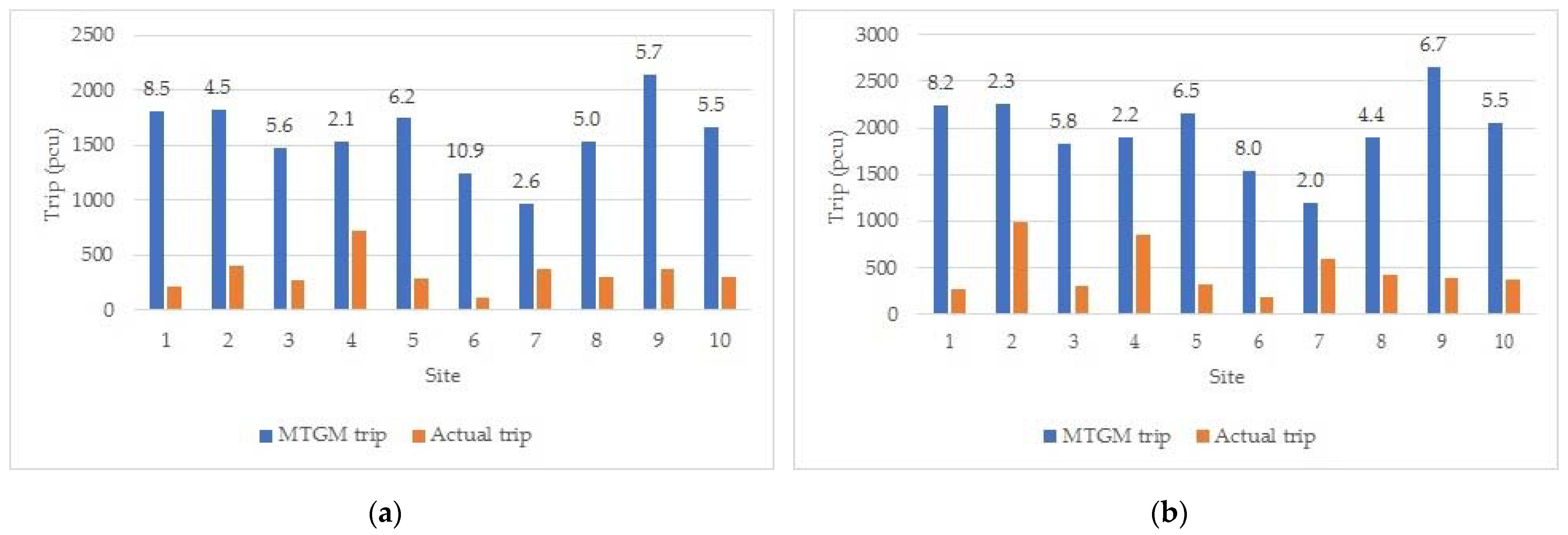
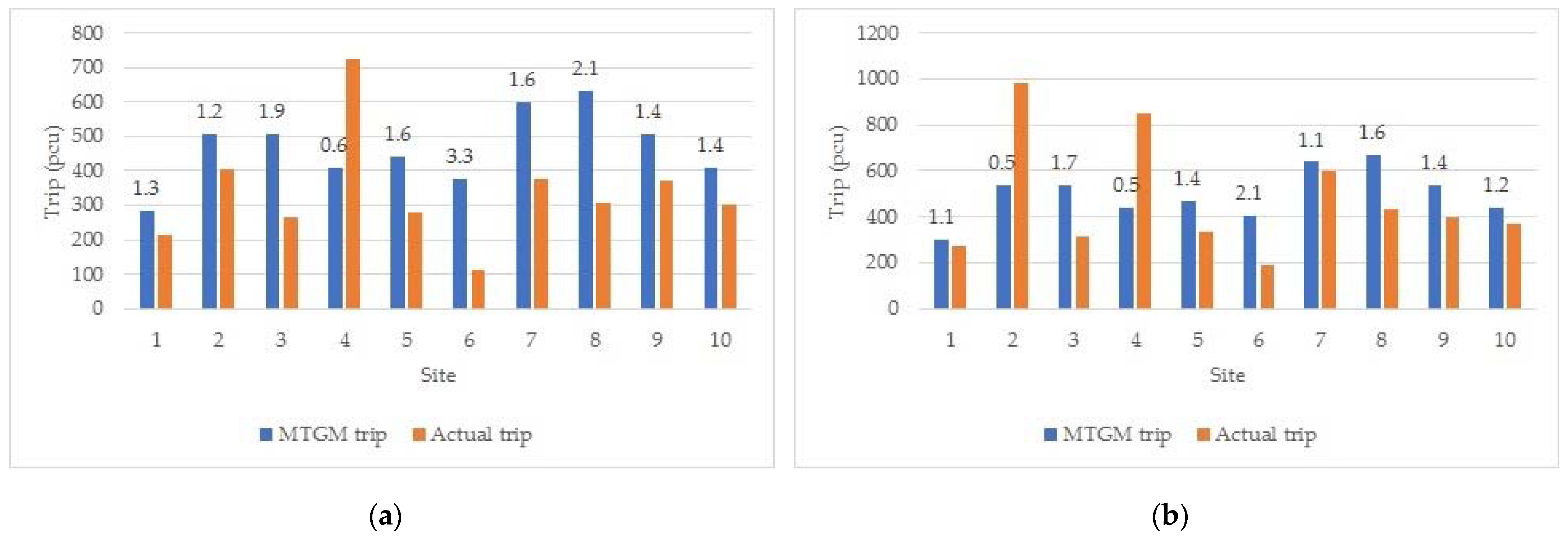
4.4. Comparison of Study Model and MTGM

The trip generation model published in the MTGM uses a simple linear regression equation. For the petrol station category, only two independent variables are used: number of pumps and GFA. Even though the number of samples in the MTGM is more than 20, the R² is still considered low at less than 13%. However, this value is higher than the R² of this study, except for the evening peak hour for which we obtained 8.3% of the variation in trips explained by the number of pumps. Besides the linear regression equation, weighted average trip is also used to forecast trip generation. The average trip rate generated in this study is also lower than the rate in the MTGM. These and other comparisons are depicted in

Table 5. Statistical comparison between this study and MTGM.

Time	Independent Variable (x)	Study				MTGM
		n 1	Equation	R2	Average Rate	n 1	Equation	R2	Average Rate
Morning peak	Pumps	10	y = 8.092x + 216.135	0.027	23.25	27	y = 5.990x + 209.443	0.033	36.21
	GFA		y = 7.241x + 266.925	0.008	36.59	22	y = −1.480x + 282.691	0.039	176.32
Evening peak	Pumps	10	y = 22.660x + 138.934	0.083	32.30	27	y = 8.401x + 194.007	0.058	36.81
	GFA		y = 4.111x + 435.146	0.001	52.05	22	y = −2.840x + 295.429	0.126	221.45

¹ n = Number of samples.

.

Based on the equations shown in Table 5, it can be concluded that the R² value derived from the regression equation of the MTGM data for petrol stations is lower than 0.50. Therefore, for this category, the manual recommends using the average rate for calculating trip generation. Trip generation estimation for the petrol stations surveyed in this study used this average rate method. There are noticeable differences in trip generation estimation values for independent variable GFA using average rate against actual trips observed during peak hours, as depicted in Figure 5. The number of estimated trips is larger by 2.1 to 10.9 times than the number of trips observed during the morning peak, and for the evening peak it is 2.0 to 8.2 times larger. Sites 4 and 7 show the smallest differences between estimated trips and actual trips, with only 2.1 and 2.6 times larger estimates for their morning peaks and 2.2 and 2.0 times larger estimates for their evening peaks. On the other hand, the largest differences were recorded at sites 1 and 6, with 8.5 and 10.9 times larger estimates for their morning peaks and 8.2 and 8.0 times larger estimates for their evening peaks.

As for the number of pumps as an independent variable, trip estimation figures are bigger than the actual counts from most sites, in between 1.2 and 2.1 times larger for morning peaks and 1.1 and 2.1 times larger for evening peaks. This is shown in Figure 6. Thus, trip generation rates calculated using the number of pumps variable are closer to the actual numbers of trips observed as compared to trip generation rate estimates based on GFA. Moreover, there was one site for which the MTGM estimation was less than the trips counted during the morning peak hour and two sites that had real tallies that were similar to the estimates for their evening peak hours. At site 2, the actual trips counted during the evening peak was double the estimated figure. The trip estimates for site 4 were about 60 percent less than the actual number of trips during the morning peak and 50 percent less than those during the evening peak.

5. Conclusions

In summary, the findings from this study show that the trip generation model using the number of seats at the fast-food restaurant as an independent variable had the highest value of R² (compared with models using total GFA and number of pumps). On the other hand, the multiple regression model with all three independent variables generated the best value of R² among all of the models applied in this study. Even though the R² value is still below the satisfactory level, this study managed to provide a foundation for further studies to create a valid multiple regression model for this new land use category to be included in the MTGM. This approach can be used for other developments, such as mixed-use buildings that combine more than one land use category such as residential units together with commercial units.

In this preliminary study, data were only collected from selected stations in Penang state and Klang Valley. Thus, the sample data are insufficient. Since this land use category is still new and developing, most of the existing petrol stations do not fulfil the requirements needed for this study, and therefore not many petrol stations are available for data collection. Furthermore, we encountered a few station owners who were reluctant to participate in this study. Therefore, it is recommended to collect more data from different petrol stations across the country for future study to ensure that more comprehensive statistical analysis can be performed to validate the model. In addition, with adequate data, future study would be able to explore other non-linear regression methods for more complicated data and analysis.

Apart from the small number of samples involved in this study, there might be other variables affecting trip generation for petrol stations with convenience stores and fast-food restaurants. Independent variables to be taken into consideration in future studies are the average daily traffic on adjacent roads, site location and density of petrol stations. In addition, socioeconomic and demographic factors should also be considered in order to improve the trip generation model for this category.

The number of vehicles on the road network in our country has continued to increase each year. As a result, demand for petrol and other related services will keep on increasing and this will lead to new petrol stations opening nationwide. It has recently become a popular trend that new petrol stations provide other services, such as convenience stores and fast-food restaurants. Federal and state governments, together with local authorities, should create a policy to encourage this type of land use combination to reduce vehicular trip, thereby reducing road congestion and carbon emissions. With the availability of good models, forecasting trips will become more accurate and road sustainability could be maintained.

References

1. Morimoto, A. Traffic and safety sciences: Interdisciplinary wisdom of IATSS. In Traffic and Safety Sciences: Interdisciplinary Wisdom of IATSS; International Association of Traffic and Safety Sciences: Tokyo, Japan, 2015; pp. 22–30. ISBN 978-4-9900252-3-6. [Google Scholar]
2. Kazaura, W.G.; Burra, M.M. Land Use Change and Traffic Impact Analysis in Planned Urban Areas in Tanzania: The Case of Dar Es Salaam City. Curr. Urban Stud. 2017, 5, 1–19. [Google Scholar] [CrossRef] [Green Version]
3. Science Daily. Available online: https://www.sciencedaily.com/terms/filling_station.htm (accessed on 15 August 2021).
4. A&W. All American Food. Available online: https://www.awfranchising.com/2019/07/why-aw-is-a-great-brand-for-your-convenience-store-or-gas-station/ (accessed on 15 August 2021).
5. Goh, B. MarketScreener. Available online: https://www.marketscreener.com/quote/stock/CHINA-PETROLEUM-CHEMICA-6497363/news/Yum-China-to-open-KFC-outlets-at-Chinese-gas-stations-28150581/ (accessed on 15 August 2021).
6. Lim, J. Restaurant Operator Collaborates with Petroleum Company to Widen Reach. 2018. Available online: https://www.thestar.com.my/metro/metro-news/2018/05/19/more-options-for-food-and-fuel-restaurant-operator-collaborates-with-petroleum-company-to-widen-reac (accessed on 24 August 2021).
7. Highway Planning Unit Ministry of Works. Malaysia Trip Generation Manual; Highway Planning Unit: Kuala Lumpur, Malaysia, 2010. [Google Scholar]
8. Shi, F.; Zhu, L. Analysis of Trip Generation Rates in Residential Commuting Based on Mobile Phone Signaling Data. J. Transp. Land Use 2019, 12, 201–220. [Google Scholar] [CrossRef]
9. Kasikoen, K.M.; Syafwandi; Hardiyani, R.; Lisnawati, S. Calculation of Trip Generation of Industrial Activities around Legok Street in Tangerang District. Int. J. Innov. Creat. Chang. 2020, 13, 1051–1070. [Google Scholar]
10. Al-Sahili, K.; Eisheh, S.A.; Kobari, F. Estimation of New Development Trip Impacts through Trip Generation Rates for Major Land Uses in Palestine. Jordan J. Civ. Eng. 2018, 12, 669–682. [Google Scholar]
11. Jayasinghe, A.; Sano, K.; Rattanaporn, K. Application for Developing Countries: Estimating Trip Attraction in Urban Zones Based on Centrality. J. Traffic Transp. Eng. (Engl. Ed.) 2017, 4, 464–476. [Google Scholar] [CrossRef]
12. Anggraini, R.; Sugiarto, S.; Pramanda, H. Factors Affecting Trip Generation of Motorcyclist for the Purpose of Non-Mandatory Activities. In Proceedings of the 3rd International Conference on Construction and Building Engineering (ICONBUILD), Palembang, Indonesia, 14–17 August 2017; AIP Publishing: Palembang, Indoneisa, 2017; Volume 1903, p. 060011. [Google Scholar]
13. Altaher, M.G.M.; Abdallah, A.M.; Elsayed, M.A.; Baz, A.E.; Abd, B.; Mahfouz, E.-S. Creating Trip Generation Models for Unplanned Cities. Int. J. Sci. Eng. Res. 2019, 10, 396–406. [Google Scholar]
14. Aboelenen, K.E.; Mohammad, A.N.; Elgaar, M.I.; Choe, P. Trip Generation Rates Using Household Surveys in the State of Qatar. J. Traffic Logist. Eng. 2021, 9, 10–19. [Google Scholar] [CrossRef]
15. Kulpa, T.; Szarata, A. Analysis of Household Survey Sample Size in Trip Modelling Process. In Proceedings of the 6th Transport Research Arena, Warsaw, Poland, 18–21 April 2016; Elsevier, B.V.: Krakow, Poland, 2016; Volume 14, pp. 1753–1761. [Google Scholar]
16. Breyer, N. Methods for Travel Pattern Analysis Using Large-Scale Passive Data; Linköping University Electronic Press: Norrköping, Sweden, 2021. [Google Scholar]
17. Llorca, C.; Ji, J.; Molloy, J.; Moeckel, R. The Usage of Location Based Big Data and Trip Planning Services for the Estimation of a Long-Distance Travel Demand Model. Predicting the Impacts of a New High Speed Rail Corridor. Res. Transp. Econ. 2018, 72, 27–36. [Google Scholar] [CrossRef]
18. Millard-Ball, A. Phantom Trips: Overestimating the Traffic Impacts of New Development. J. Transp. Land Use 2015, 8, 31–49. [Google Scholar] [CrossRef] [Green Version]
19. WisDOT. Convenience Store Gas Station Interim Guidance; Bureau of Traffic Operations WisDOT Division of Transportation System Development: Madison, WI, USA, 2021. [Google Scholar]
20. Florida Department of Transportation. Trip Generation: Characteristics of Large Gas Stations/Convenience Stores and Student Apartments; Florida Department of Transportation: Tallahassee, FL, USA, 2012. [Google Scholar]
21. Akinsulire, E.O.; Fadare, S.O. An Assessment on the Locational Pattern of Petrol Filling Stations along Lasu-Isheri Road Corridor. Am. Int. J. Multidiscip. Sci. Res. 2020, 6, 6–29. [Google Scholar] [CrossRef]
22. Mahmoudi, J. Trip Generation Characteristics of Super Convenience Market—Gasoline Pump Stores. ITE J. 2012, 82, 16–21. [Google Scholar]
23. Utainarumola, S.; Ampawasuvanb, S. Fuel Station Trips Generation on Arterial Road in Thailand: A Case Study in Chonburi Province. Int. J. Eng. Innov. Technol. 2018, 8, 14–20. [Google Scholar] [CrossRef]
24. Cunningham, C.M.; Findley, D.J.; Schroeder, B.; Foyle, R.S. Traffic Operational Impacts of Contemporary Multi-Pump Island Fueling Centers. ITE J. 2011, 81, 24–33. [Google Scholar]
25. Patel, B.V.; Kadiya, D.K.; Varia, H.R. Developing Industrial Trip Generation Model for Himatnagar Industrial Area. Int. J. Eng. Res. Technol. (IJERT) 2017, 6, 768–775. [Google Scholar]
26. Yulianto, B.; Prasetyo, R.A. Study of Standard Trip Attraction Models of Various Land Use in the Surakarta City. J. Phys. Conf. Ser. 2020, 1625, 12037. [Google Scholar] [CrossRef]
27. Al-Masaeid, H.R.; Fayyad, S.S. Estimation of Trip Generation Rates for Residential Areas in Jordan. Jordan J. Civ. Eng. 2018, 12, 162–172. [Google Scholar]
28. Hameed Naser, I.; Shaia, H. Estimation Trip Generation for Urban Area of Nasiriyh City. J. Glob. Sci. Res. 2020, 3, 451–460. [Google Scholar]
29. Moeckel, R.; Huntsinger, L.; Donnelly, R. From Macro to Microscopic Trip Generation: Representing Heterogeneous Travel Behavior. Open Transp. J. 2017, 11, 31–43. [Google Scholar] [CrossRef] [Green Version]
30. Huntsinger, L.F.; Rouphail, N.M.; Bloomfield, P. Trip Generation Models Using Cumulative Logistic Regression. J. Urban Plan. Dev. 2013, 139, 176–184. [Google Scholar] [CrossRef]
31. Nguyen, H.N.T.; Chikaraishi, M.; Fujiwara, A.; Zhang, J. Exploring the Influence of Social Capital at Different Levels on Trip Generation and Destination Choice for Discretionary Activities. J. East. Asia Soc. Transp. Stud. 2017, 12, 2345–2361. [Google Scholar] [CrossRef]
32. Gim, T.H.T. Analysing the Effects of Land Use on the Choice of Intra-Zonal Trip Destinations—A Comparison Between Weekday and Weekend Travel. Promet–Traffic Transp. 2020, 32, 527–542. [Google Scholar] [CrossRef]
33. Garrett, M. Encyclopedia of Transportation: Social Science and Policy; Garrett, M., Ed.; SAGE Publications, Inc.: Los Angeles, CA, USA, 2014; Volume 1, ISBN 148334651X. [Google Scholar]
34. Minhans, A.; Zaki, N.H.; Shahid, S.; Abdelfatah, A. A Comparison of Deterministic and Stochastic Approaches for the Estimation of Trips Rates. J. Transp. Syst. Eng. 2014, 1, 1–11. [Google Scholar]
35. Bureau of Traffic Operations Wisconsin Department of Transportation. Traffic Impact Analysis Guidelines; Bureau of Traffic Operations Wisconsin Department of Transportation: Madison, WI, USA, 2021. [Google Scholar]
36. Ahmed, I.; Abdulrahman, S.; Hainin, M.R.; Hassan, S.A. Trip Generations at “Polyclinic” Land Use Type in Johor Bahru, Malaysia. Promet-Traffic Transp. 2014, 26, 467–473. [Google Scholar] [CrossRef] [Green Version]
37. Asad, F.H. Travel Demand Forecasting Using UK TRICS Database. J. Intell. Transp. Urban Plan. 2015, 3, 98–107. [Google Scholar] [CrossRef] [Green Version]
38. Road & Maritime Services Transport for NSW TDT 2013/04a Guide to Traffic Generating Developments Updated Traffic Surveys. 2013. Available online: https://roads-waterways.transport.nsw.gov.au/trafficinformation/downloads/td13-04a.pdf (accessed on 24 August 2021).
39. Trips Database Bureau—Transportation Group NZ. Available online: https://www.transportationgroup.nz/trips-database-bureau/ (accessed on 23 August 2021).
40. Hamzah, M.O.; Sadullah, A.F.M.; Mat, H.; Osman, A.; Leong, L.V.; Mohd Shafie, S.A.; Jusoh, J. Trip Generation Study Phase Iv; Final Report; Universiti Sains Malaysia: Nibong Tebal, Malaysia, 2009. [Google Scholar]
41. Mohd Shafie, S.A. Pembentukan Model Alternatif Untuk Model Penjanaan Perjalanan Malaysia Bagi Guna Tanah Perumahan, Institusi, Pendidikan Dan Komersial. Master’s Thesis, Universiti Sains Malaysia, Penang, Malaysia, June 2011. [Google Scholar]
42. Schneider, R.J.; Shafizadeh, K.; Handy, S.L. Method to Adjust Institute of Transportation Engineers Vehicle Trip-Generation Estimates in Smart-Growth Areas. J. Transp. Land Use 2015, 8, 69–83. [Google Scholar] [CrossRef] [Green Version]
43. Jabatan Perangkaan Malaysia. Taburan Penduduk dan Ciri-ciri Asas Demografi 2010. Available online: https://www.mycensus.gov.my/index.php/ms/produk-banci/penerbitan/banci-2010/664-taburan-penduduk-dan-ciri-ciri-asas-demografi-2010 (accessed on 24 October 2021).
44. Institute of Transportation Engineers (ITE). Trip Generation Manual; Institute of Transportation Engineers (ITE): Washington, DC, USA, 2012. [Google Scholar]
45. Semih, T.; Seyhan, S. A Multi-Criteria Factor Evaluation Model for Gas Station Site Selection. J. Glob. Manag. 2011, 2, 12–21. [Google Scholar]
46. Lam, W.S.; Lam, W.H.; Liew, K.F.; Chen, J.W. An Empirical Study on the Preference of Fast Food Restaurants in Malaysia with AHP-TOPSIS Model. J. Eng. Appl. Sci. 2018, 13, 3226–3231. [Google Scholar] [CrossRef]
47. Sharif, S.; Lwee, X.Y. Measuring Market Share of Petrol Stations Using Conditional Probability Approach. In Proceedings of the International Conference on Education, Mathematics and Science 2016 (ICEMS2016) in conjunction with the 4th International Postgraduate Conference on Science and Mathematics 2016 (IPCSM2016), Tanjung Malim, Perak, Malaysia, 19 November 2016; AIP Publishing: New York, NY, USA, 2017; Volume 1847, p. 020014. [Google Scholar]
48. Islam, N.; Ullah, G.M.S. Factors Affecting Consumers’ Preferences on Fast Food Items in Bangladesh. J. Appl. Bus. Res. 2010, 26, 131–146. [Google Scholar] [CrossRef]
49. Al-Madadhah, A.; Imam, R. Developing Trip Generation Rates for Restaurants in Amman. Int. J. Inf. Bus. Manag. 2020, 12, 69–80. [Google Scholar]
50. Barbara, I.; Susan, D. Introductory Statistics; OpenStax: Houston, TX, USA, 2013. [Google Scholar]
51. Ahmed, I.; Abdulameer, A.; Puan, O.C.; Minhans, A. Trip Generation at Fast—Food Restaurants in Johor Bahru, Malaysia. J. Teknol. 2014, 70, 91–95. [Google Scholar] [CrossRef] [Green Version]
52. Das, K.R.; Rahmatullah Imon, A.H.M. A Brief Review of Tests for Normality. Am. J. Theor. Appl. Stat. 2016, 5, 5–12. [Google Scholar] [CrossRef] [Green Version]
53. Arimie, C.O.; Biu, E.O.; Ijomah, M.A. Outlier Detection and Effects on Modeling. Open Access Libr. J. 2020, 7, e6619. [Google Scholar] [CrossRef]
54. Shrestha, N. Detecting Multicollinearity in Regression Analysis. Am. J. Appl. Math. Stat. 2020, 8, 39–42. [Google Scholar] [CrossRef]
Figure 1. Study methodology.
Sustainability 13 12815 g001
Figure 2. Traffic volume fluctuations at all sites.
Sustainability 13 12815 g002
Figure 3. Trip volume comparison per hour for two adjacent sites. (a) Traffic volume fluctuations at site 6 and site 7. (b) Traffic volume fluctuations at site 5 and site 8.
Sustainability 13 12815 g003aSustainability 13 12815 g003b
Figure 4. Trip generation model: (a) number of pumps as the independent variable, (b) GFA as the independent variable, (c) number of restaurant seats as the independent variable.
Sustainability 13 12815 g004
Figure 5. Comparison between estimated trip volume calculated using average trip rate according to GFA and actual trip volume calculated at the surveyed site during peak hours: (a) comparison at morning peak, (b) comparison at evening peak.
Sustainability 13 12815 g005
Figure 6. Comparison between estimated trip volume calculated using average trip rate according to number of pumps and actual trip volume calculated at the surveyed site during peak hours: (a) comparison at morning peak, (b) comparison at evening peak.
Sustainability 13 12815 g006