
The Effects of Rock Index Tests on Prediction of Tensile Strength of Granitic Samples: A Neuro-Fuzzy Intelligent System


 ,
, 

 and
and
Abstract
:1. Introduction
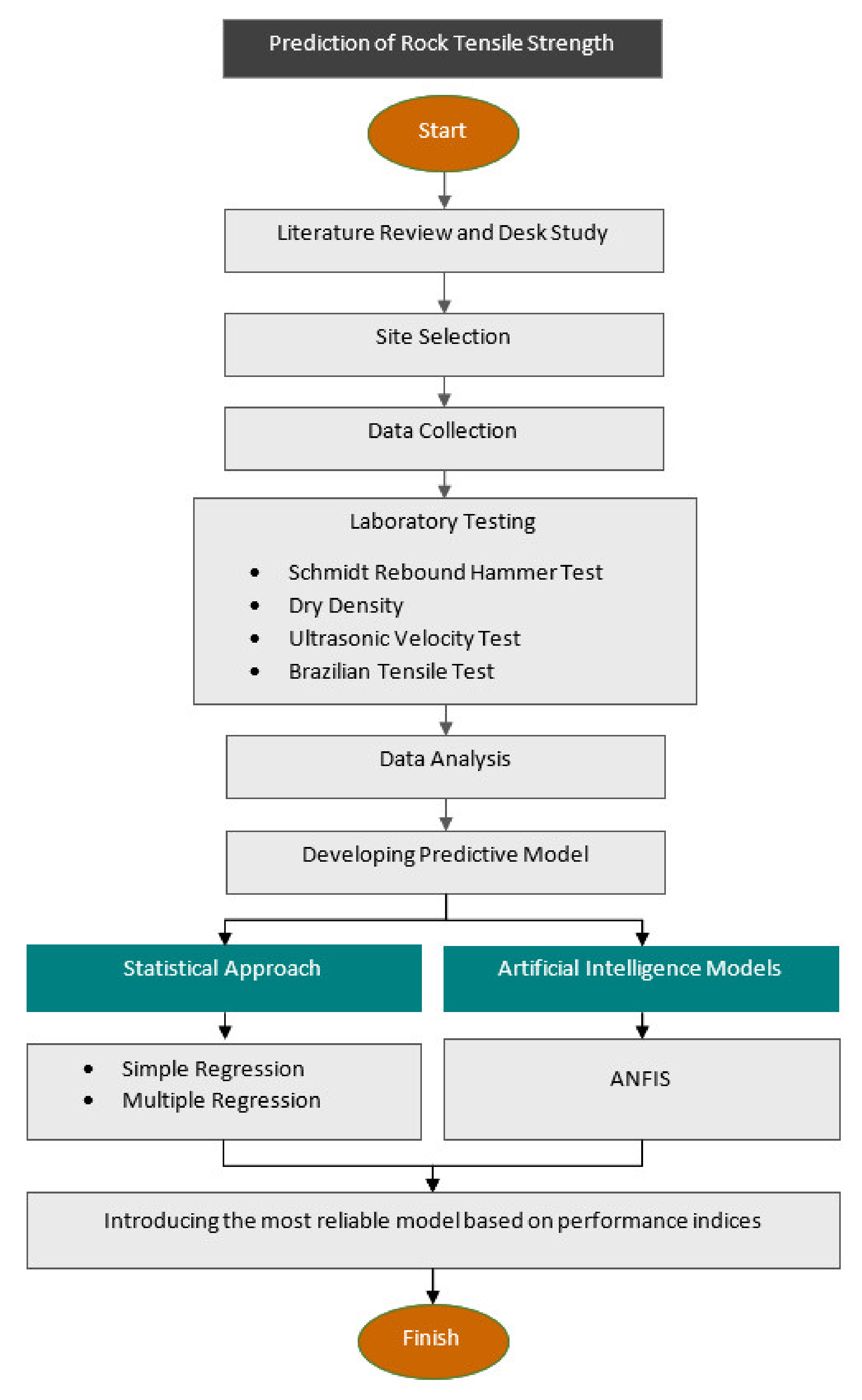
2. Methods and Material
2.1. Laboratory Tests
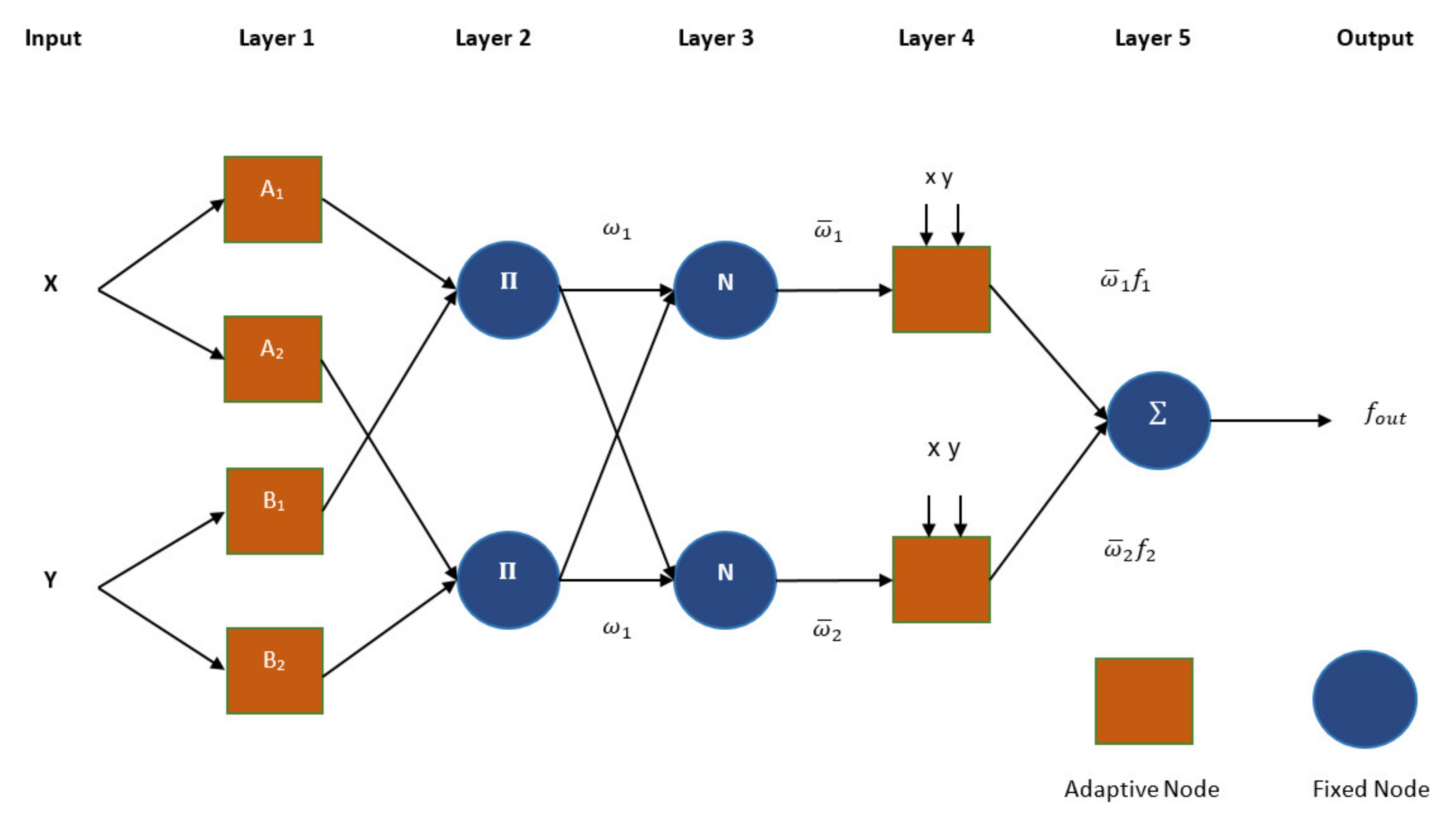
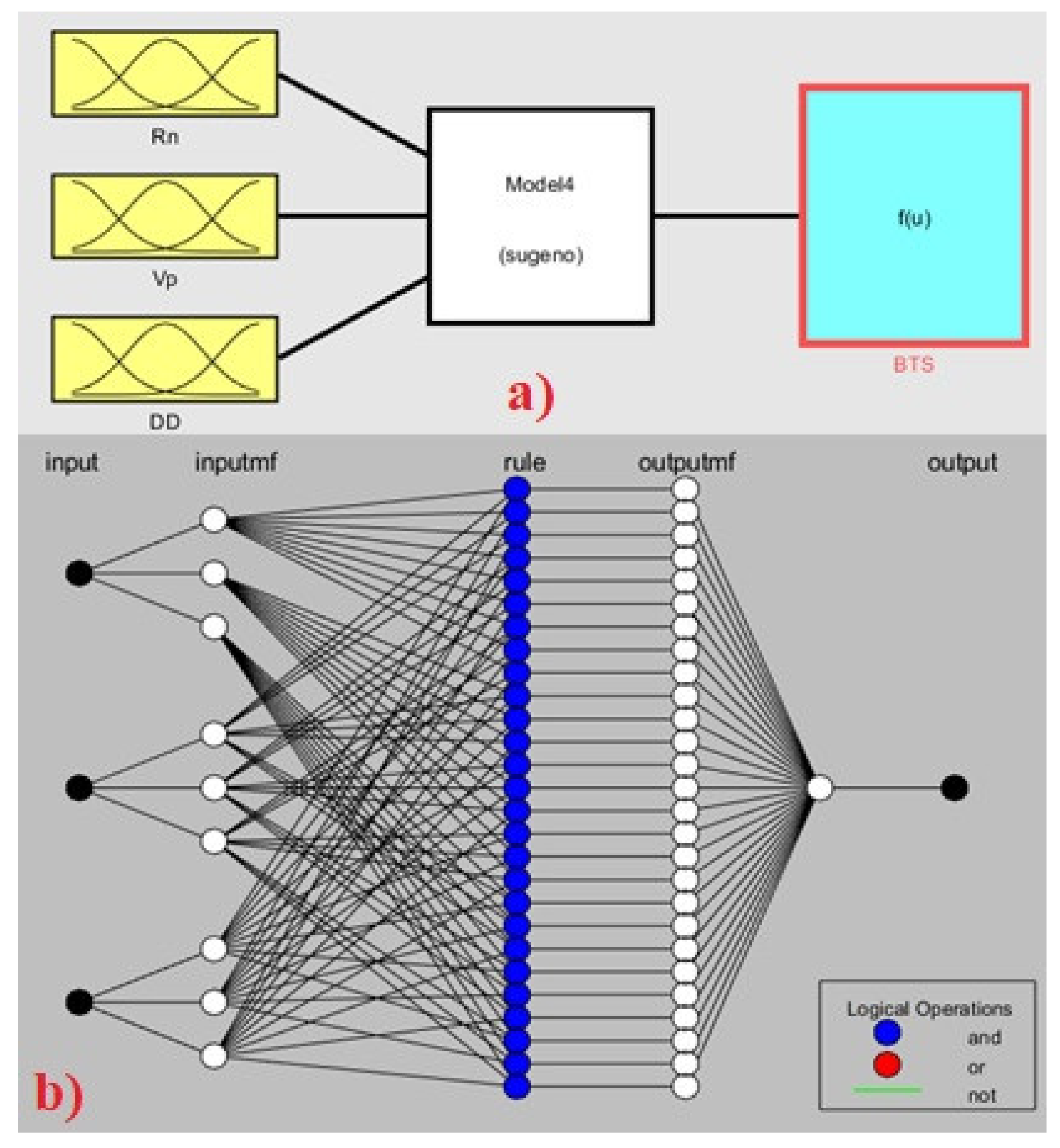
2.2. ANFIS Background
- Layer 1 (fuzzy layer): Comprises adaptive nodes with functions expressed (Equations (3) and (4)) as:where and indicate the input nodes, and denotes the linguistic labels, implies the MFs.
- Layer 2 (product layer): Includes the product layer of two fixed nodes labelled expressed as Equation (5).
- Layer 3 (normalised layer): Node function is to normalise the weight function of the following process and is labelled as N, Equation (6):
- Layer 4 (defuzzy layer): Contains adaptive nodes marked by a square, Equation (7):
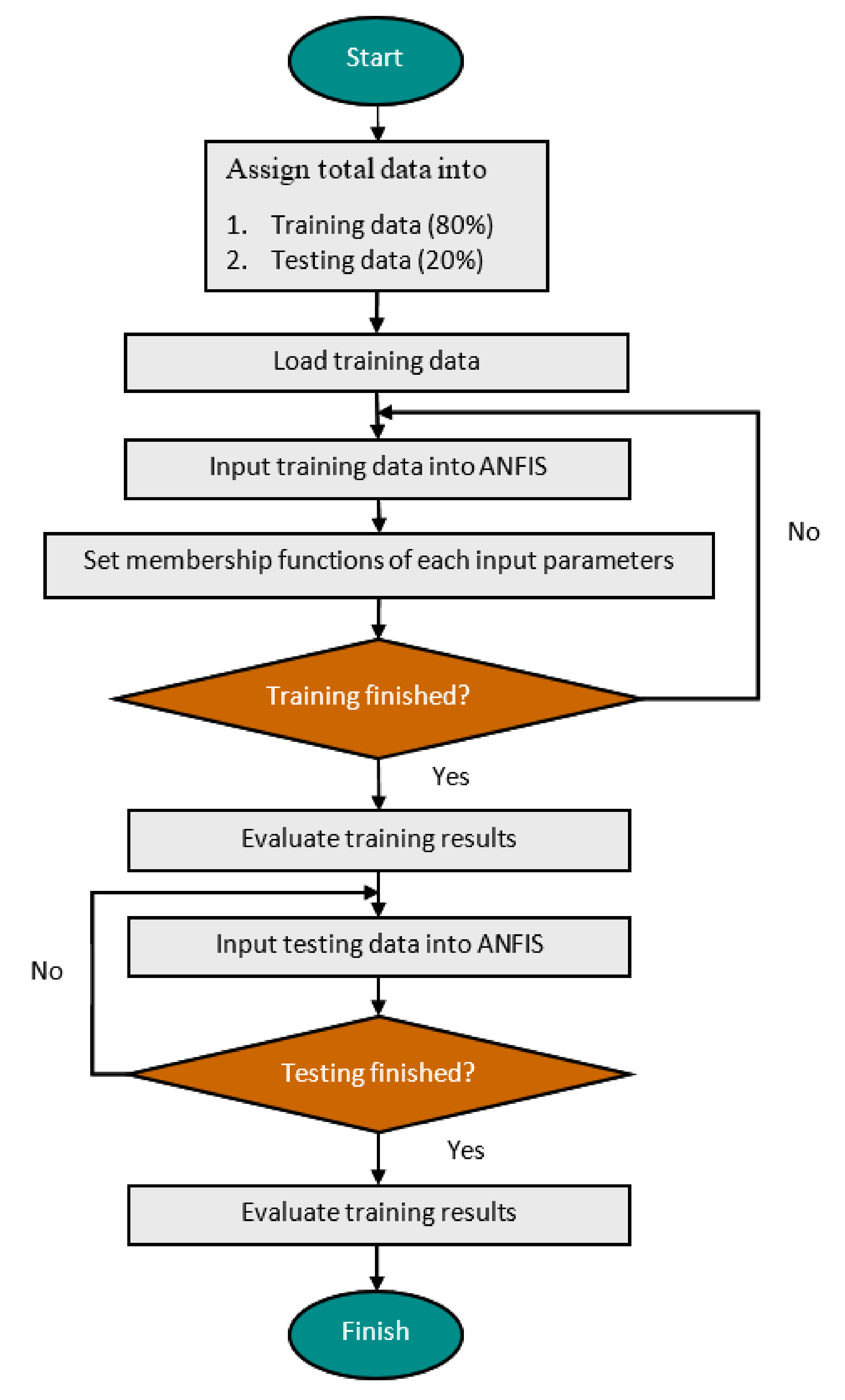
- Layer 5 (total output layer): Contains fixed node with function to compute overall output, Equation (8):where denotes the output of each layer and represents the weight function of the next layer. Figure 1 illustrates the architecture of ANFIS. In addition, the overview of ANFIS flowchart is illustrated in Figure 2.
2.3. Step-by-Step Overview of Research
2.4. Statistical Index
3. Modelling, Analysis, and Results
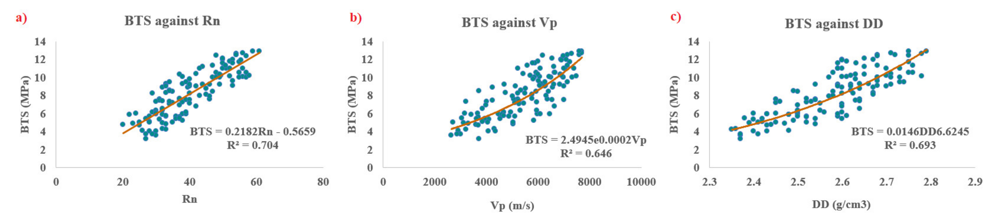
3.1. SR Modelling
3.2. MLR Modelling
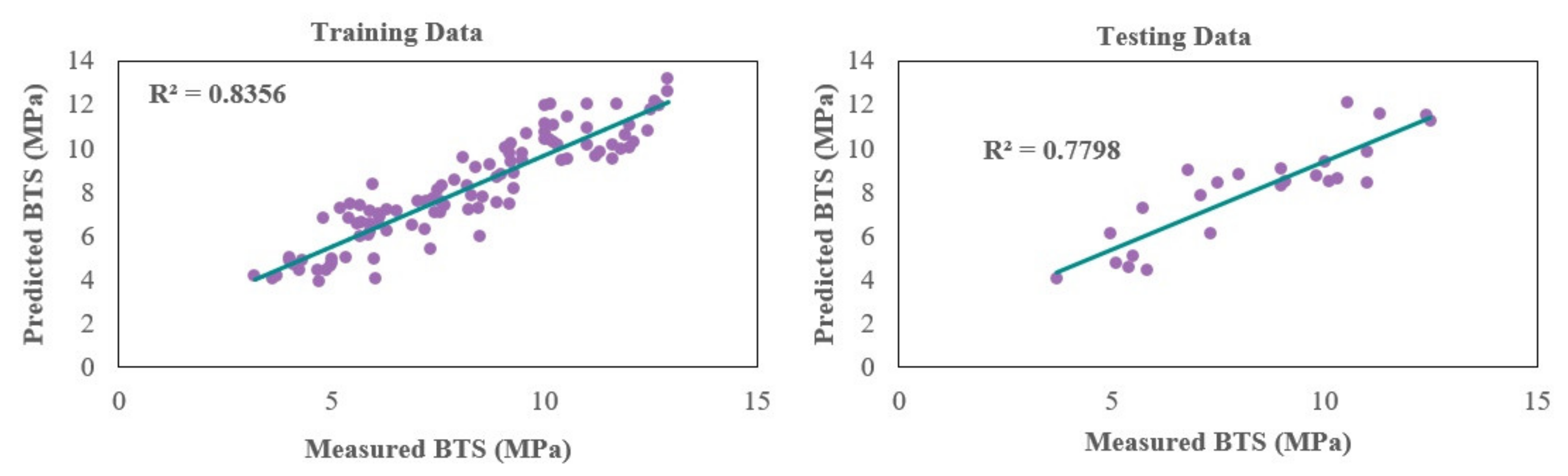
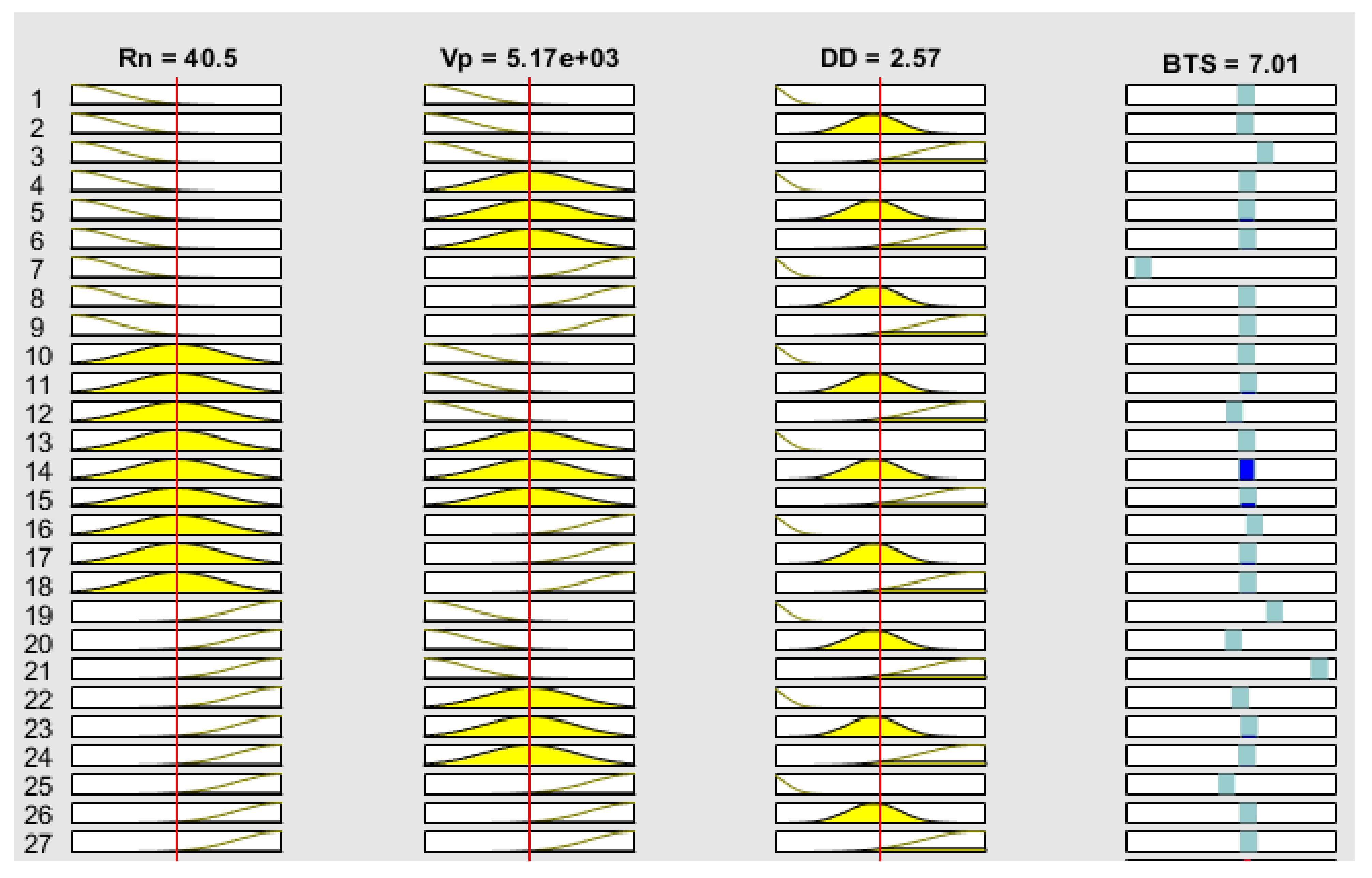
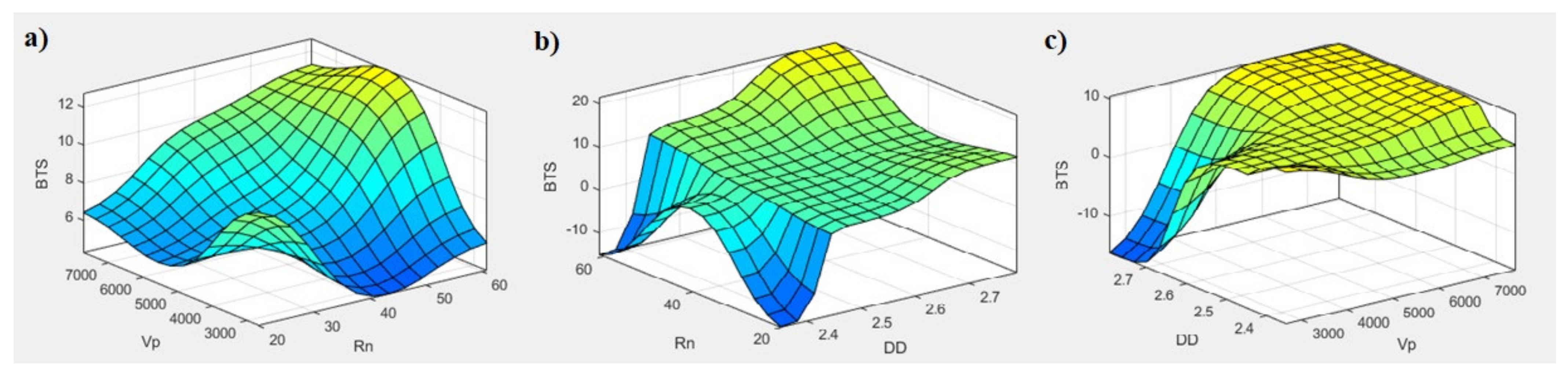
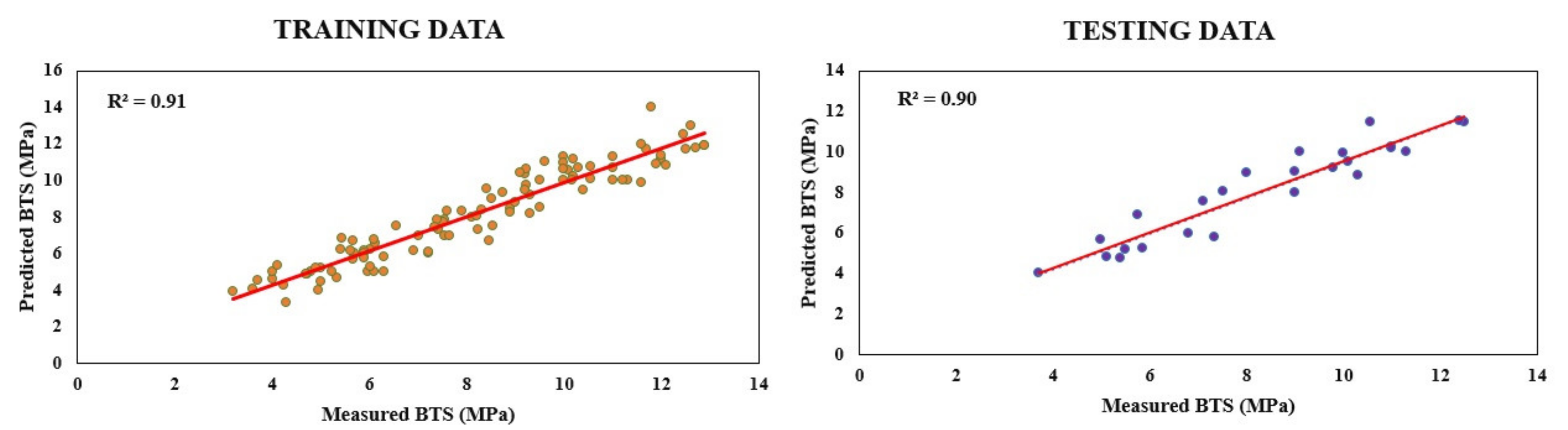
3.3. ANFIS Modelling
4. Discussion
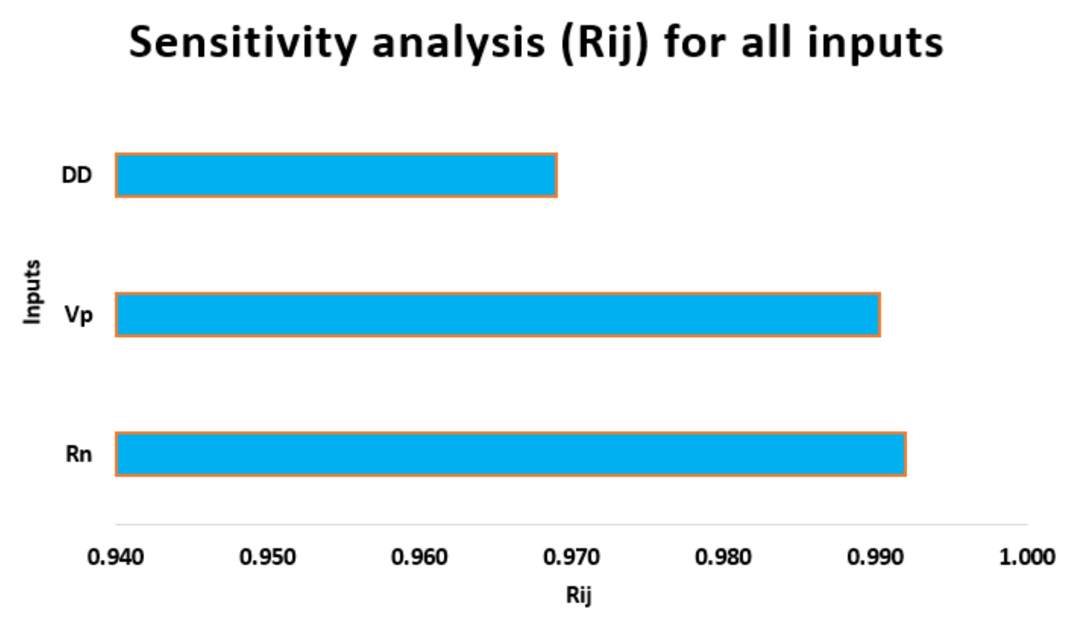
5. Sensitivity Analysis
6. Limitations and Future Works
7. Conclusions
Author Contributions
Funding
Institutional Review Board Statement
Informed Consent Statement
Data Availability Statement
Acknowledgments
Conflicts of Interest
Appendix A

| Sample No. | Rn | Vp (m/s) | DD (g/cm3) | BTS (MPa) |
| 1 | 33 | 4670 | 2.61 | 5.75 |
| 2 | 34 | 3210 | 2.53 | 7.34 |
| 3 | 52 | 6102 | 2.59 | 11 |
| 4 | 54 | 7155 | 2.68 | 12.5 |
| 5 | 43 | 5217 | 2.59 | 11 |
| 6 | 42 | 6635 | 2.6 | 6.8 |
| 7 | 33 | 6080 | 2.68 | 9.1 |
| 8 | 57 | 6980 | 2.68 | 12.4 |
| 9 | 40 | 7003 | 2.54 | 7.5 |
| 10 | 27 | 3615 | 2.42 | 5.4 |
| 11 | 22 | 3430 | 2.48 | 5.85 |
| 12 | 37 | 6005 | 2.65 | 10.3 |
| 13 | 40 | 5832 | 2.63 | 9.8 |
| 14 | 50.8 | 7152 | 2.76 | 11.3 |
| 15 | 28 | 3866 | 2.42 | 5.1 |
| 16 | 48 | 6503 | 2.57 | 10 |
| 17 | 38 | 6430 | 2.6 | 10.1 |
| 18 | 37 | 3050 | 2.38 | 5.5 |
| 19 | 43 | 6320 | 2.58 | 7.99 |
| 20 | 57 | 6659 | 2.76 | 10.55 |
| 21 | 28 | 5040 | 2.52 | 4.99 |
| 22 | 29 | 2870 | 2.37 | 3.7 |
| 23 | 40 | 5463 | 2.55 | 7.1 |
| 24 | 42 | 7002 | 2.59 | 8.99 |
| 25 | 33 | 5125 | 2.7 | 9 |
References
- Wu, H.; Kemeny, J.; Wu, S. Experimental and numerical investigation of the punch-through shear test for mode II fracture toughness determination in rock. Eng. Fract. Mech. 2017, 184, 59–74. [Google Scholar] [CrossRef]
- Demirdag, S.; Tufekci, K.; Sengun, N.; Efe, T. Determination of the Direct Tensile Strength of Granite Rock by Using a New Dumbbell Shape and its Relationship with Brazilian Tensile Strength Determination of the Direct Tensile Strength of Granite Rock by Using a New Dumbbell Shape and its Relationship. In IOP Conference Series: Earth and Environmental Science; IOP Publishing: Bristol, UK, 2019. [Google Scholar]
- Li, D.; Wong, L.N.Y. The brazilian disc test for rock mechanics applications: Review and new insights. Rock Mech. Rock Eng. 2013, 46, 269–287. [Google Scholar] [CrossRef]
- He, W.; Chen, K.; Zhang, B.; Dong, K. Improving Measurement Accuracy of Brazilian Tensile Strength of Rock by Digital Image Correlation. Rev. Sci. Instrum. 2018, 89, 115107. [Google Scholar] [CrossRef] [PubMed]
- Yao, W.; Xia, K.; Li, X. Non-Local Failure Theory and Two-Parameter Tensile Strength Model for Semi-Circular Bending Tests of Granitic Rocks. Int. J. Rock Mech. Min. Sci. 2018, 110, 9–18. [Google Scholar] [CrossRef]
- Choi, B.H.; Lee, Y.K.; Park, C.; Ryu, C.H.; Park, C. Measurement of Tensile Strength of Brittle Rocks Using a Half Ring Shaped Specimen. Geosci. J. 2019, 23, 649–660. [Google Scholar] [CrossRef]
- Xia, K.; Yao, W.; Wu, B. Dynamic Rock Tensile Strengths of Laurentian Granite: Experimental Observation and Micromechanical Model. J. Rock Mech. Geotech. Eng. 2017, 9, 116–124. [Google Scholar] [CrossRef]
- Xu, X.; Wu, S.; Gao, Y.; Xu, M. Effects of Micro-structure and Micro-parameters on Brazilian Tensile Strength Using Flat-Joint Model. Rock Mech. Rock Eng. 2016, 49, 3575–3595. [Google Scholar] [CrossRef]
- Yuan, R.; Shen, B. Numerical Modelling of the Contact Condition of a Brazilian Disk Test and Its Influence on the Tensile Strength of Rock. Int. J. Rock Mech. Min. Sci. 2017, 93, 54–65. [Google Scholar] [CrossRef]
- Ma, Y.; Huang, H. DEM Analysis of Failure Mechanisms in The Intact Brazilian Test. Int. J. Rock Mech. Min. Sci. 2018, 102, 109–119. [Google Scholar] [CrossRef]
- Aydin, A.; Basu, A. The Schmidt hammer in rock material characterization. Eng. Geol. 2005, 81, 1–14. [Google Scholar] [CrossRef]
- Liao, Z.Y.; Zhu, J.B.; Tang, C.A. Numerical investigation of rock tensile strength determined by direct tension, Brazilian and three-point bending tests. Int. J. Rock Mech. Min. Sci. 2019, 115, 21–32. [Google Scholar] [CrossRef]
- Briševac, Z.; Kujundžić, T.; Čajić, S. Sadašnje spoznaje o ispitivanju vlačne čvrstoće stijena uporabom Brazilskoga testa. Rud.-Geol.-Naft. Zb. 2015, 30, 101–114. [Google Scholar]
- Nazir, R.; Momeni, E.; Armaghani, D.J.; Amin, M.F.M. Correlation between unconfined compressive strength and indirect tensile strength of limestone rock samples. Electron. J. Geotech. Eng. 2013, 18, 1737–1746. [Google Scholar]
- Kabilan, N. Correlation between Unconfined Compressive Strength and Indirect Tensile Strength for Jointed Rocks. Int. J. Res. Eng. Technol. 2016, 5, 157–161. [Google Scholar]
- Jahed Armaghani, D.; Mohd Amin, M.F.; Yagiz, S.; Faradonbeh, R.S.; Abdullah, R.A. Prediction of the uniaxial compressive strength of sandstone using various modeling techniques. Int. J. Rock Mech. Min. Sci. 2016, 85, 174–186. [Google Scholar] [CrossRef]
- Jahed Armaghani, D.; Hajihassani, M.; Yazdani Bejarbaneh, B.; Marto, A.; Tonnizam Mohamad, E. Indirect measure of shale shear strength parameters by means of rock index tests through an optimized artificial neural network. Meas. J. Int. Meas. Confed. 2014, 55, 487–498. [Google Scholar] [CrossRef]
- Heidari, M.; Khanlari, G.R.; Kaveh, M.T.; Kargarian, S. Predicting the Uniaxial Compressive and Tensile Strengths of Gypsum Rock by Point Load Testing. Rock Mech. Rock Eng. 2012, 45, 265–273. [Google Scholar] [CrossRef]
- Altindag, R.; Guney, A. Predicting the relationships between brittleness and mechanical properties (UCS, TS and SH) of rocks. Sci. Res. Essays 2010, 5, 2107–2118. [Google Scholar]
- Farah, R. Correlations between Index Properties and Unconfined Compressive Strength of Weathered Ocala Limestone. Master’s Thesis, University North Florida, Jacksonville, FL, USA, 2011. [Google Scholar]
- Kahraman, S.; Fener, M.; Kozman, E. Predicting the compressive and tensile strength of rocks from indentation hardness index. J. South. Afr. Inst. Min. Metall. 2012, 112, 331–339. [Google Scholar]
- Mohamad, E.T.; Armaghani, D.J.; Momeni, E.; Abad, S.V.A.N.K. Prediction of the unconfined compressive strength of soft rocks: A PSO-based ANN approach. Bull. Eng. Geol. Environ. 2015, 74, 745–757. [Google Scholar] [CrossRef]
- Khandelwal, M.; Faradonbeh, R.S.; Monjezi, M.; Armaghani, D.J.; Majid, M.Z.B.A.; Yagiz, S. Function development for appraising brittleness of intact rocks using genetic programming and non-linear multiple regression models. Eng. Comput. 2017, 33, 13–21. [Google Scholar] [CrossRef]
- Mahdiyar, A.; Armaghani, D.J.; Marto, A.; Nilashi, M.; Ismail, S. Rock Tensile Strength Prediction Using Empirical and Soft Computing Approaches. Bull. Eng. Geol. Environ. 2019, 78, 4519–4531. [Google Scholar] [CrossRef]
- Liu, B.; Yang, H.; Karekal, S. Effect of Water Content on Argillization of Mudstone during the Tunnelling process. Rock Mech. Rock Eng. 2019, 53, 799–813. [Google Scholar] [CrossRef]
- Yang, H.; Wang, H.; Zhou, X. Analysis on the damage behavior of mixed ground during TBM cutting process. Tunn. Undergr. Space Technol. 2016, 57, 55–65. [Google Scholar] [CrossRef]
- Zhou, J.; Qiu, Y.; Khandelwal, M.; Zhu, S.; Zhang, X. Developing a hybrid model of Jaya algorithm-based extreme gradient boosting machine to estimate blast-induced ground vibrations. Int. J. Rock Mech. Min. Sci. 2021, 145, 104856. [Google Scholar] [CrossRef]
- Zhou, J.; Li, X.; Mitri, H.S. Classification of rockburst in underground projects: Comparison of ten supervised learning methods. J. Comput. Civ. Eng. 2016, 30, 4016003. [Google Scholar] [CrossRef]
- Armaghani, D.J.; Hajihassani, M.; Mohamad, E.T.; Marto, A.; Noorani, S.A. Blasting-induced flyrock and ground vibration prediction through an expert artificial neural network based on particle swarm optimization. Arab. J. Geosci. 2014, 7, 5383–5396. [Google Scholar] [CrossRef]
- Zhang, W.; Wu, C.; Zhong, H.; Li, Y.; Wang, L. Prediction of undrained shear strength using extreme gradient boosting and random forest based on Bayesian optimization. Geosci. Front. 2021, 12, 469–477. [Google Scholar] [CrossRef]
- Zhang, W.G.; Li, H.R.; Wu, C.Z.; Li, Y.Q.; Liu, Z.Q.; Liu, H.L. Soft computing approach for prediction of surface settlement induced by earth pressure balance shield tunneling. Undergr. Space 2020, 6, 353–363. [Google Scholar] [CrossRef]
- Zhang, W.; Li, H.; Li, Y.; Liu, H.; Chen, Y.; Ding, X. Application of deep learning algorithms in geotechnical engineering: A short critical review. Artif. Intell. Rev. 2021, 1–41. [Google Scholar] [CrossRef]
- Yang, H.; Wang, Z.; Song, K. A new hybrid grey wolf optimizer-feature weighted-multiple kernel-support vector regression technique to predict TBM performance. Eng. Comput. 2020, 1–17. [Google Scholar] [CrossRef]
- Armaghani, D.J.; Mohamad, E.T.; Narayanasamy, M.S.; Narita, N.; Yagiz, S. Development of hybrid intelligent models for predicting TBM penetration rate in hard rock condition. Tunn. Undergr. Space Technol. 2017, 63, 29–43. [Google Scholar] [CrossRef]
- Park, S.-S.; Ogunjinmi, P.D.; Woo, S.-W.; Lee, D.-E. A Simple and Sustainable Prediction Method of Liquefaction-Induced Settlement at Pohang Using an Artificial Neural Network. Sustainability 2020, 12, 4001. [Google Scholar] [CrossRef]
- Mohammed, A.S.; Asteris, P.G.; Koopialipoor, M.; Alexakis, D.E.; Lemonis, M.E.; Armaghani, D.J. Stacking Ensemble Tree Models to Predict Energy Performance in Residential Buildings. Sustainability 2021, 13, 8298. [Google Scholar] [CrossRef]
- Gowida, A.; Moussa, T.; Elkatatny, S.; Ali, A. A hybrid artificial intelligence model to predict the elastic behavior of sandstone rocks. Sustainability 2019, 11, 5283. [Google Scholar] [CrossRef] [Green Version]
- Yang, H.Q.; Lan, Y.F.; Lu, L.; Zhou, X.P. A quasi-three-dimensional spring-deformable-block model for runout analysis of rapid landslide motion. Eng. Geol. 2015, 185, 20–32. [Google Scholar] [CrossRef]
- Zhou, J.; Shen, X.; Qiu, Y.; Li, E.; Rao, D.; Shi, X. Improving the efficiency of microseismic source locating using a heuristic algorithm-based virtual field optimization method. Geomech. Geophys. Geo-Energy Geo-Resour. 2021, 7, 89. [Google Scholar] [CrossRef]
- Zhou, J.; Chen, C.; Wang, M.; Khandelwal, M. Proposing a novel comprehensive evaluation model for the coal burst liability in underground coal mines considering uncertainty factors. Int. J. Min. Sci. Technol. 2021, 18. [Google Scholar] [CrossRef]
- Singh, V.K.; Singh, D.; Singh, T.N. Prediction of strength properties of some schistose rocks from petrographic properties using artificial neural networks. Int. J. Rock Mech. Min. Sci. 2001, 38, 269–284. [Google Scholar] [CrossRef]
- Çanakci, H.; Baykasoǧlu, A.; Güllü, H. Prediction of compressive and tensile strength of Gaziantep basalts via neural networks and gene expression programming. Neural Comput. Appl. 2009, 18, 1031–1041. [Google Scholar] [CrossRef]
- Ceryan, N.; Okkan, U.; Samul, P.; Ceryan, S. Modeling of tensile strength of rocks based on support vector machines approaches. Int. J. Numer. Anal. Methods Geomech. 2012, 37, 2655–2670. [Google Scholar] [CrossRef]
- Gurocak, Z.; Solanki, P.; Alemdag, S.; Zaman, M.M. New considerations for empirical estimation of tensile strength of rocks. Eng. Geol. 2012, 144–145, 1–8. [Google Scholar] [CrossRef]
- Huang, L.; Asteris, P.G.; Koopialipoor, M.; Armaghani, D.J.; Tahir, M.M. Invasive Weed Optimization Technique-Based ANN to the Prediction of Rock Tensile Strength. Appl. Sci. 2019, 9, 5372. [Google Scholar] [CrossRef] [Green Version]
- ISRM Turkish National Group. The Complete ISRM Suggested Methods for Rock Characterization, Testing and Monitoring: 1974–2006; ISRM Turkish National Group: Ankara, Turkey, 2009. [Google Scholar]
- Armaghani, D.J.; Mohamad, E.T.; Momeni, E.; Narayanasamy, M.S. An adaptive neuro-fuzzy inference system for predicting unconfined compressive strength and Young’s modulus: A study on Main Range granite. Bull. Eng. Geol. Environ. 2015, 74, 1301–1319. [Google Scholar] [CrossRef]
- Çaydaş, U.; Hasçalik, A.; Ekici, S. An adaptive neuro-fuzzy inference system (ANFIS) model for wire-EDM. Expert Syst. Appl. 2009, 36, 6135–6139. [Google Scholar] [CrossRef]
- Lo, S.P. The application of an ANFIS and grey system method in turning tool-failure detection. Int. J. Adv. Manuf. Technol. 2002, 19, 564–572. [Google Scholar] [CrossRef]
- Armaghani, D.J.; Harandizadeh, H.; Momeni, E.; Maizir, H.; Zhou, J. An optimized system of GMDH-ANFIS predictive model by ICA for estimating pile bearing capacity. Artif. Intell. Rev. 2021, 1–38. [Google Scholar] [CrossRef]
- Armaghani, D.J.; Mohamad, E.T.; Hajihassani, M.; Yagiz, S.; Motaghedi, H. Application of several non-linear prediction tools for estimating uniaxial compressive strength of granitic rocks and comparison of their performances. Eng. Comput. 2016, 32, 189–206. [Google Scholar] [CrossRef]
- Willmott, C.J.; Matsuura, K. Advantages of the mean absolute error (MAE) over the root mean square error (RMSE) in assessing average model performance. Clim. Res. 2005, 30, 79–82. [Google Scholar] [CrossRef]
- Menard, S. Coefficients of determination for multiple logistic regression analysis. Am. Stat. 2000, 54, 17–24. [Google Scholar]
- Xu, H.; Zhou, J.; Asteris, P.G.; Jahed Armaghani, D.; Tahir, M.M. Supervised Machine Learning Techniques to the Prediction of Tunnel Boring Machine Penetration Rate. Appl. Sci. 2019, 9, 3715. [Google Scholar] [CrossRef] [Green Version]
- Bai, Q.S.; Tu, S.H.; Zhang, C. DEM investigation of the fracture mechanism of rock disc containing hole(s) and its influence on tensile strength. Theor. Appl. Fract. Mech. 2016, 86, 197–216. [Google Scholar] [CrossRef]
- Kumar, B.R.; Vardhan, H.; Govindaraj, M. Prediction of Uniaxial Compressive Strength, Tensile Strength and Porosity of Sedimentary Rocks Using Sound Level Produced During Rotary Drilling. Rock Mech. Rock Eng. 2011, 44, 613–620. [Google Scholar] [CrossRef]
- Gokceoglu, C.; Zorlu, K. A fuzzy model to predict the uniaxial compressive strength and the modulus of elasticity of a problematic rock. Eng. Appl. Artif. Intell. 2004, 17, 61–72. [Google Scholar] [CrossRef]
- Liang, M.; Mohamad, E.T.; Faradonbeh, R.S.; Jahed Armaghani, D.; Ghoraba, S. Rock strength assessment based on regression tree technique. Eng. Comput. 2016, 32, 343–354. [Google Scholar] [CrossRef]
- Hasanipanah, M.; Zhang, W.; Armaghani, D.J.; Rad, H.N. The potential application of a new intelligent based approach in predicting the tensile strength of rock. IEEE Access 2020, 8, 57148–57157. [Google Scholar] [CrossRef]
- Al-Hmouz, A.; Shen, J.; Al-Hmouz, R.; Yan, J. Modeling and simulation of an Adaptive Neuro-Fuzzy Inference System (ANFIS) for mobile learning. IEEE Trans. Learn. Technol. 2012, 5, 226–237. [Google Scholar] [CrossRef]
- Zorlu, K.; Gokceoglu, C.; Ocakoglu, F.; Nefeslioglu, H.A.; Acikalin, S. Prediction of uniaxial compressive strength of sandstones using petrography-based models. Eng. Geol. 2008, 96, 141–158. [Google Scholar] [CrossRef]


| References | Proposed Equations | Regression Type | R2 | Description |
|---|---|---|---|---|
| Heidari et al. [18] | L | 0.9 | 40 Gypsum rocks | |
| Altindag and Guney [19] | NL | 0.8 | 143 rock samples | |
| Farah [20] | NL | 0.6 | 195 of limestone specimens | |
| Kahraman et al. [21] | L | 0.5 | Igneous rocks | |
| Nazir et al. [14] | NL | 0.9 | 40 laboratory strength tests on dry limestone | |
| Mohamad et al. [22] | L | 0.8 | 40 sets soft rock samples | |
| Khandelwal et al. [23] | NL | 0.9 | 13 types of rock from USA | |
| Mahdiyar et al. [24] | NL | 0.7 | 100 granite block samples | |
| Mahdiyar et al. [24] | NL | 0.7 | 100 granite block samples |
| References | Model | Input Parameters | Model Performance | Description |
|---|---|---|---|---|
| Singh et al. [41] | ANN | Petrographical characteristics | MAPE = 11% | Schistose rocks |
| Çanakci et al. [42] | ANN | Vp, DD, Rn, WA | R2 = 0.99 | 86 samples of basalt from Turkey |
| Gurocak et al. [44] | MLPN | Is50, Rn, γ | R2 = 0.84 | 174 samples from Turkey |
| Ceryan et al. [43] | LS-SVM | POR, Vp, SDI, aggregate impact | R2 = 0.86 | 55 carbonate rocks from Turkey |
| Mahdiyar et al. [24] | PSO-ANN | Is50, DD, Rn | R2 = 0.93 | Granite rock samples |
| Huang et al. [45] | IWO-ANN | Is50, DD, Rn | R2 = 0.92 | 100 granite samples |
| Parameters Symbol | Group | Unit | Min | Max | Ave. | Sd. |
|---|---|---|---|---|---|---|
| Rn | Input | - | 20 | 61 | 40.5 | 9.93 |
| Vp | Input | m/s | 2643 | 7702 | 5172.5 | 1331.60 |
| DD | Input | g/cm3 | 2.35 | 2.79 | 2.57 | 0.11 |
| BTS | Output | MPa | 3.2 | 12.9 | 8.05 | 2.58 |
| Model | Input | Equation Type | Equation | R2 | Rank |
|---|---|---|---|---|---|
| 1 | Rn | Exponential | 0.657 | 1 | |
| Linear | 0.704 | 4 | |||
| Logarithmic | 0.690 | 3 | |||
| Power | 0.659 | 2 | |||
| 2 | Vp | Exponential | 0.646 | 4 | |
| Linear | 0.638 | 2 | |||
| Logarithmic | 0.611 | 1 | |||
| Power | 0.638 | 2 | |||
| 3 | DD | Exponential | 0.689 | 3 | |
| Linear | 0.670 | 1 | |||
| Logarithmic | 0.671 | 2 | |||
| Power | 0.693 | 4 |
| Model No. | Input | Equation |
|---|---|---|
| MR1 | Vp, DD | |
| MR2 | Rn, DD | |
| MR3 | Rn, Vp | |
| MR4 | Rn, Vp, DD |
| Model No. | Training Data | Training Ranking | Total Rank | ||||||
|---|---|---|---|---|---|---|---|---|---|
| RMSE | VAF (%) | R2 | a20-Index | RMSE | VAF | R2 | a20-Index | ||
| MR1 | 1.24 | 76.97 | 0.77 | 0.75 | 1 | 1 | 1 | 1 | 4 |
| MR2 | 1.09 | 82.17 | 0.82 | 0.84 | 3 | 3 | 3 | 3 | 12 |
| MR3 | 1.22 | 77.75 | 0.78 | 0.75 | 2 | 2 | 2 | 1 | 7 |
| MR4 | 1.05 | 83.56 | 0.84 | 0.84 | 4 | 4 | 4 | 3 | 15 |
| Model No. | Testing Data | Testing Ranking | Total Rank | ||||||
|---|---|---|---|---|---|---|---|---|---|
| RMSE | VAF (%) | R2 | a20-Index | RMSE | VAF | R2 | a20-Index | ||
| MR1 | 1.43 | 67.42 | 0.68 | 0.72 | 1 | 1 | 1 | 1 | 4 |
| MR2 | 1.18 | 78.94 | 0.79 | 0.76 | 4 | 4 | 4 | 3 | 15 |
| MR3 | 1.39 | 70.13 | 0.71 | 0.72 | 2 | 2 | 2 | 1 | 7 |
| MR4 | 1.20 | 77.87 | 0.78 | 0.80 | 3 | 3 | 3 | 4 | 13 |
| Model Name | Input | Output | Epoch | |
|---|---|---|---|---|
| MF No. | MF Type | MF Type | ||
| Model 1 | 222 | Bell Membership | Constant | 117 |
| Model 2 | 333 | Bell Membership | Constant | 10 |
| Model 3 | 222 | Gaussian | Constant | 23 |
| Model 4 | 333 | Gaussian | Constant | 88 |
| Model 5 | 222 | Gaussian 2 | Constant | 17 |
| Model 6 | 333 | Gaussian 2 | Constant | 6 |
| Model 7 | 222 | Bell Membership | Linear | 9 |
| Model 8 | 222 | Gaussian 2 | Linear | 10 |
| Model Name | Training Datasets | Testing Datasets | ||||||||||||||||
|---|---|---|---|---|---|---|---|---|---|---|---|---|---|---|---|---|---|---|
| Statistical Index | Rank | Total | Statistical Index | Rank | Total | |||||||||||||
| RMSE | VAF (%) | R2 | a20-Index | RMSE | VAF | R2 | a20-Index | RMSE | VAF (%) | R2 | a20-Index | RMSE | VAF | R2 | a20-Index | |||
| Model 1 | 0.98 | 85.69 | 0.86 | 0.89 | 3 | 3 | 5 | 5 | 16 | 1.10 | 81.19 | 0.81 | 0.84 | 7 | 7 | 6 | 7 | 27 |
| Model 2 | 0.90 | 87.90 | 0.88 | 0.91 | 5 | 5 | 6 | 7 | 23 | 1.39 | 69.74 | 0.88 | 0.73 | 1 | 2 | 7 | 4 | 14 |
| Model 3 | 1.01 | 84.80 | 0.85 | 0.87 | 2 | 2 | 4 | 3 | 11 | 1.15 | 79.37 | 0.79 | 0.80 | 5 | 5 | 4 | 6 | 20 |
| Model 4 | 0.70 | 90.53 | 0.91 | 0.92 | 8 | 8 | 8 | 8 | 32 | 0.84 | 89.68 | 0.90 | 0.96 | 8 | 8 | 8 | 8 | 32 |
| Model 5 | 1.01 | 84.73 | 0.85 | 0.88 | 2 | 1 | 4 | 4 | 11 | 1.14 | 79.50 | 0.80 | 0.84 | 6 | 6 | 5 | 7 | 22 |
| Model 6 | 0.96 | 86.40 | 0.86 | 0.90 | 4 | 4 | 5 | 6 | 19 | 1.38 | 69.43 | 0.71 | 0.76 | 2 | 1 | 2 | 5 | 10 |
| Model 7 | 0.85 | 89.20 | 0.89 | 0.88 | 7 | 7 | 7 | 4 | 25 | 1.32 | 71.82 | 0.73 | 0.84 | 3 | 3 | 3 | 7 | 16 |
| Model 8 | 0.86 | 89.05 | 0.89 | 0.91 | 6 | 6 | 7 | 7 | 26 | 1.19 | 78.56 | 0.79 | 0.80 | 4 | 4 | 4 | 6 | 18 |
| Number of Layers | 5 |
| Training Data Size | 102 × 4 |
| Testing Data Size | 25 × 4 |
| FIS Properties | Grid Partition |
| Input FIS Structure | |
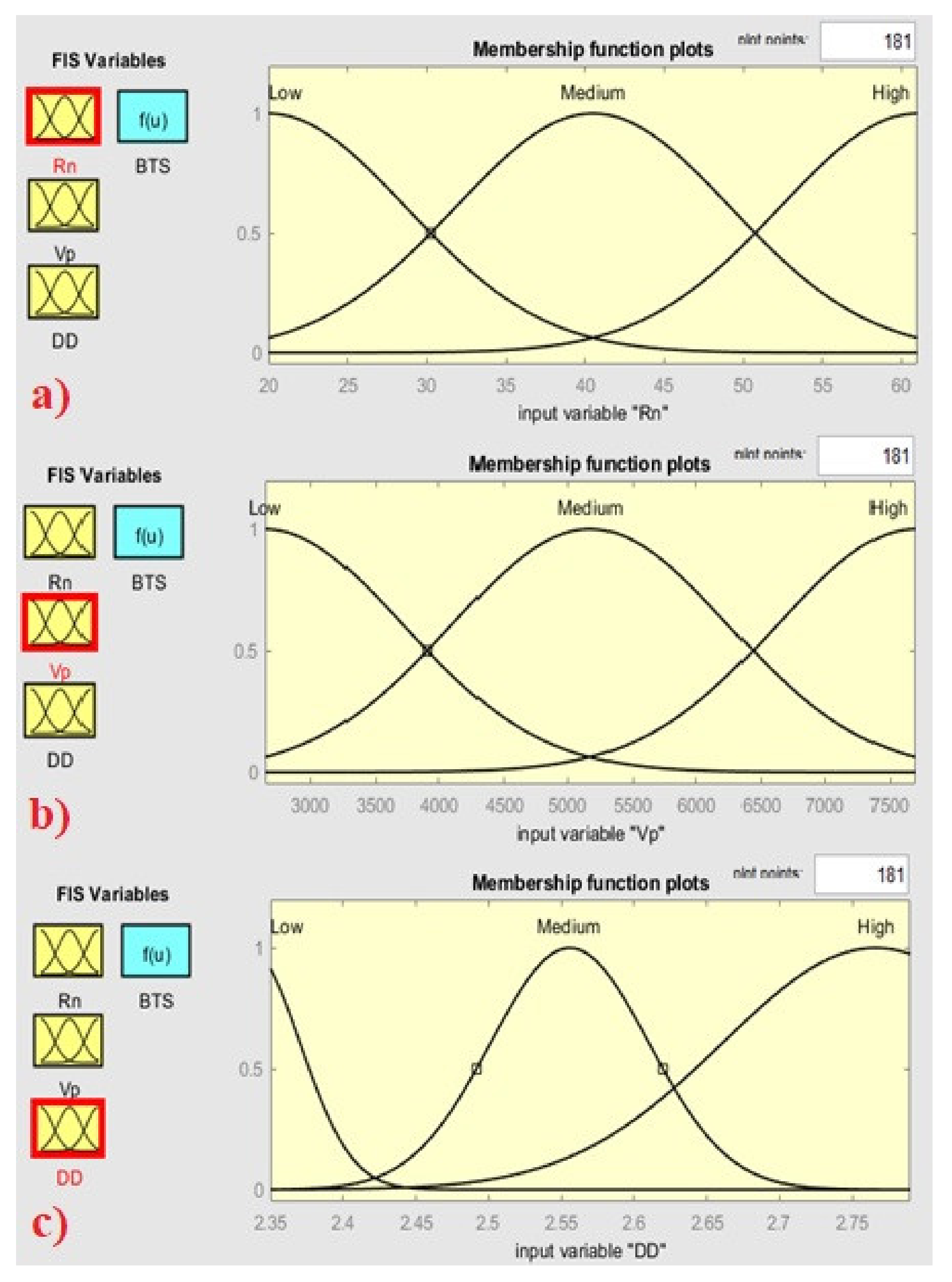
| MF Type | Gaussian |
| MF Number | 333 |
| Output FIS Structure | |
| MF Type | Constant |
| FIS Training | |
| Optimum Method | Hybrid |
| Error Tolerance | 0 |
| Epochs Number | 88 |
| FIS System | |
| Input | 3 |
| Output | 1 |
| Rules Number | 27 |
| Model Name | Train | Test | ||||||
|---|---|---|---|---|---|---|---|---|
| RMSE | VAF (%) | R2 | a20-Index | RMSE | VAF (%) | R2 | a20-Index | |
| ANFIS Model | 0.70 | 90.53 | 0.91 | 0.96 | 0.84 | 89.68 | 0.90 | 0.96 |
| MLR4 | 1.05 | 83.56 | 0.84 | 0.84 | 1.20 | 77.87 | 0.78 | 0.80 |
Publisher’s Note: MDPI stays neutral with regard to jurisdictional claims in published maps and institutional affiliations. |
© 2021 by the authors. Licensee MDPI, Basel, Switzerland. This article is an open access article distributed under the terms and conditions of the Creative Commons Attribution (CC BY) license (https://creativecommons.org/licenses/by/4.0/).
Share and Cite
Li, Y.; Hishamuddin, F.N.S.; Mohammed, A.S.; Armaghani, D.J.; Ulrikh, D.V.; Dehghanbanadaki, A.; Azizi, A. The Effects of Rock Index Tests on Prediction of Tensile Strength of Granitic Samples: A Neuro-Fuzzy Intelligent System. Sustainability 2021, 13, 10541. https://doi.org/10.3390/su131910541
Li Y, Hishamuddin FNS, Mohammed AS, Armaghani DJ, Ulrikh DV, Dehghanbanadaki A, Azizi A. The Effects of Rock Index Tests on Prediction of Tensile Strength of Granitic Samples: A Neuro-Fuzzy Intelligent System. Sustainability. 2021; 13(19):10541. https://doi.org/10.3390/su131910541
Chicago/Turabian StyleLi, Yan, Fathin Nur Syakirah Hishamuddin, Ahmed Salih Mohammed, Danial Jahed Armaghani, Dmitrii Vladimirovich Ulrikh, Ali Dehghanbanadaki, and Aydin Azizi. 2021. "The Effects of Rock Index Tests on Prediction of Tensile Strength of Granitic Samples: A Neuro-Fuzzy Intelligent System" Sustainability 13, no. 19: 10541. https://doi.org/10.3390/su131910541