Multi-Criteria Analysis of Green Bonds: Hybrid Multi-Method Applications

Abstract

There is an increasing pressure by the community and customers forcing companies to insert environmental concerns in their practices. To help companies initiatives, the green bonds market was created. Our research question is “How to select bonds in a growing billion-dollar market?” This paper presents a multi-criteria decision analysis (MCDA) model to enable investors identify opportunities based not only in opinions, but grounded on objective facts. Analytic hierarchy process (AHP), complex proportional assessment (COPRAS), full consistency method (FUCOM), step-wise Weights Assessment Ratio Analysis (SWARA), and technique of order preference similarity to the ideal solution (TOPSIS) are MCDA methods applied in this paper. Top-fifteen green bonds ranked by specialized media were assessed with the proposed MCDA model. Criteria included the Environmental Performance Index (EPI) proposed by Yale University, and common financial indicators as assets, risks ($\beta$), and dividends. The new ranks from MCDA are compared each other and compared with the rank published by specialized media.

1. Introduction

Developed by Yale University, the Environmental Performance Index (EPI) provides a data-drive summary of the state of sustainability around the world [1]. EPI is obtained with 32 indicators, across 11 categories under two policy objectives: ecosystem vitality and environmental health [2,3]. With EPI, it is possible to identify the greenest countries around the world.

Zooming into company-level, the increased pressures from community and environmentally conscious consumers force companies to insert environmental concerns in their management practices [4,5]. To help companies initiatives, green bonds were inserted in 2007, as bonds issued to support environmental projects [6]. As a matter of fact, the green bond market is a potential source of climate finance for developing countries [7].

Over 600 billion United States dollars (USD) were issued in green bonds in 2020, nearly doubling the 326 billion USD issued the year before [8]. This 53% growth, in a twelve-month basis, includes green, social and sustainability bonds. The multi-billion-dollar market is tracked by most popular financial services worldwide [9,10]. Nevertheless, most relevant investment funds have already moved assets on this path. The question is no longer if green bonds have a relevant market. The question is how to select bonds in this new reality. This is the main goal of this article: to offer a simple framework for bonds selection, beyond financial reports and reviews. This paper presents a multi-criteria decision analysis (MCDA) model to enable investors identify opportunities based not in opinions, but grounded on objective facts. Since green bonds are a new trend in corporate finance, the MCDA proposal for their assessment is the major novelty of this work. The application of MCDA methods allows decision-makers and policy-makers to consider the best alternative of an array of options based on multiple factors [11].

Green bonds assessment is the problem this work intents to solve. Despite there are green bonds ranked by specialized media, this paper presents alternative ranks, resulted from the application of MCDA methods. As presented in Section 2, MCDA was not previously applied in green bonds assessment. Therefore, there are two related contributions, one in the field of green bonds and another in the field of MCDA. This paper’s hypothesis is “MCDA methods may be applied for green bonds assessment”.

MCDA is divided in two branches: multi-attribute decision analysis and multi-objective decision analysis [12]. Multi-attribute deals with a finite number of alternatives, extremely, only two alternatives. Conversely, multi-objective analysis deals with larger sets of alternatives, even infinite alternatives [13]. This paper is on multi-attribute analysis, since a finite number of alternatives will be considered. This work does not deals with optimization, as for instance from an exhaustive analysis of all possible criteria and every available green bond. This is a major delimitation for this work.

There are dozens methods for MCDA [14]. Analytic hierarchy process (AHP), complex proportional assessment (COPRAS), full consistency method (FUCOM), step-wise weights assessment ratio analysis (SWARA), and technique of order preference similarity to the ideal solution (TOPSIS) are the MCDA methods applied in this paper. These methods were chosen, at first, because they are methods for multi-attribute analysis. At second, AHP and TOPSIS were chosen because they are traditional methods [15,16]. Since green bonds assessment with MCDA is unprecedented, the choice for consolidated methods sounds safer. To surpass AHP limitations, COPRAS, FUCOM, and SWARA, newer multi-attribute analysis methods [17] were also chosen to be applied. Then, the hybrid multi-method application brings strengths from traditional and newer methods, as presented in Section 3. Hybrid methods application is a new trend in MCDA literature [18,19].

Section 2 presents a literature review, highlighting the novelty of MCDA application in green bonds assessment. Section 3 presents methodology, with methods AHP, COPRAS, FUCOM, SWARA, and TOPSIS. Section 4 presents the results of the hybrid multi-method application. Section 5 presents a discussion on the main results. Finally, Section 6 presents conclusions and directions for future research.

2. Literature Review

Literature on green bonds is just beginning. The search TITLE-ABS-KEY (“green bond”) on Scopus Database resulted in only 265 documents, by 7 August 2021. None with AHP, COPRAS, FUCOM, MCDA, SWARA, and TOPSIS, in title, abstract or keywords (TITTLE-ABS-KEY). Therefore, there is a research gap on MCDA applications on green bonds. The objective of this paper is to present an MCDA model to green bonds assessment.

Table 1. Most cited publications on green bonds.

Reference	Year	Citations	Main Findings
[21]	2019	93	Low impact of investors pro-environmental preferences on bond prices.
[22]	2018	63	Green bonds have negligible diversification benefits for investors in corporate and treasury markets.
[23]	2020	49	Firm’s issuance of green bonds is beneficial to its existing shareholders.
[24]	2018	r48	Liquidity has explanatory power for the yield spread of green bonds.
[25]	2018	48	Financial and corporate green bonds trade tighter than their comparable non-green bonds, and government-related bonds on the other hand trade marginally wider.
[26]	2019	44	Green bonds are more financially convenient than non-green ones, then they can potentially play a major role in greening the economy without penalizing financially the issuers.
[27]	2019	41	The issuer’s reputation or green third-party verification are essential to reduce informational asymmetries, avoid suspicion of green bond washing, and produce relatively more convenient financing conditions.
[28]	2016	42	Asian economies should focus on reducing financial barriers towards renewable energy projects.
[6]	2016	41	A shock in the conventional bond market tends to spillover into the green bond market, where this spillover effect is variable over time.

Source: Scopus Database (2021).

presents an overview of most cited publications on green bonds. A similar overview was presented by Kucera, Vochozka and Rowland [20], for their research on the economic value added.

Publications on green bonds resulted varied findings, for instance, on benefits, on diversification, on preferences, or on volatility. The absence of MCDA in green bonds literature suggests a research gap: green bonds researches have been developed with single-criterion analyses. Therefore, this paper contributes to green bonds literature presenting an MCDA model for bonds assessment.

In this work, AHP [29] is applied to weight the criteria, with pairwise comparisons. When the set of alternatives and the set of criteria increase, the effort for the AHP application is also increased [30]. Therefore, FUCOM [31] and SWARA [32] are also applied to weight the criteria. COPRAS [33] and TOPSIS [34] are applied, in this work, to assess the alternatives, which are real green bonds.

The major topic for AHP and TOPSIS applications is supply chain management (SCM), but there are recent researches on sustainability [35]. COPRAS has been applied for the economic selection alternatives, mainly in manufacturing applications [36,37]. Literature on FUCOM and SWARA is incipient, as presented in

Table 2. Publications on MCDA.

Subject	Overall	2019	2020	2021	2021/Overall
MCDA	49,261	4638	5402	3579	7.3%
AHP	41,512	3811	4380	2833	6.8%
TOPSIS	11,227	1430	1778	1329	11.8%
COPRAS	1246	114	127	98	7.8%
SWARA	299	56	62	55	18.4%
FUCOM	53	14	15	15	28.3%

Source: Scopus Database (2021).

. FUCOM application is a new trend in MCDA applied to engineering [38,39].

As expected due their greater age, AHP and TOPSIS publications individually overcome publications on COPRAS, FUCOM, and SWARA, together. Publications on AHP started in the 1970s, on TOPSIS in the 1980s, and on COPRAS in the 1990s. SWARA was only proposed in 2010, and FUCOM in 2018.

As presented in this section, this paper increases green bonds literature with MCDA application. This works also upgrades MCDA literature combining the application of traditional methods with newer methods, in a novel theme: Green bonds assessment.

3. Methodology

3.1. Generalities

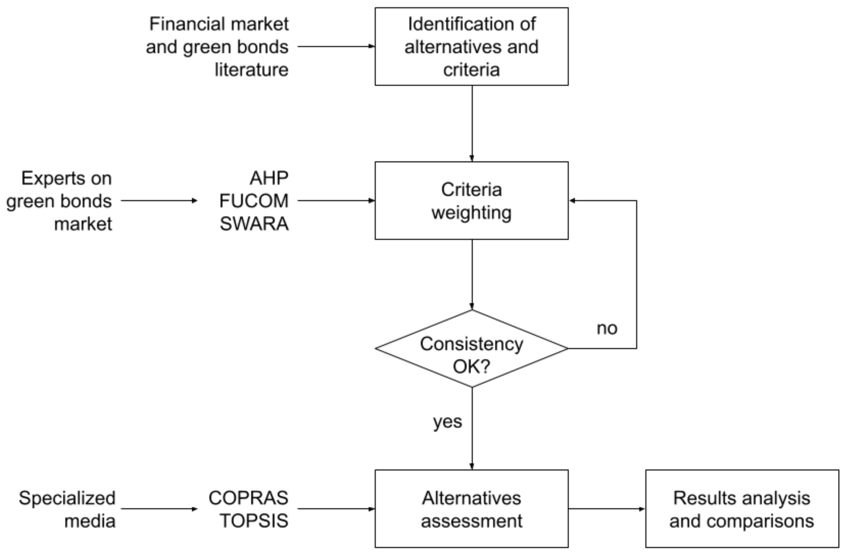
This paper presents combined applications of different methods of MCDA in the assessment of green bonds. Figure 1 presents the steps of the proposed research methodology, inside the boxes of a flow-chart.

In the first step, the criteria and alternatives for multi-criteria analysis are identified with data and information collected from literature on financial markets and green bonds. The next step is weighting the criteria with applications of AHP, FUCOM, and SWARA. If data provided by experts were not consistent, in the AHP application, inconsistent data needs to be revised. If the consistency is okay, next step is the assessment of alternatives (green bonds) with COPRAS and TOPSIS. In the final step, green bonds ranking with MCDA is compared with Kiplinger’s rank [40]. Kiplinger is a North-American media outlet specialized in investments forecasts and analysis, founded in Washington, DC, back in the 1920s, and nowadays part of the Dennis Publishing Ltd., a British independent corporation. Kiplinger’s rank is similar to Benzinga’s, Bloomberg’s, and Stock Rover’s, to name a few. While most data regarding bonds trade are usually charged [41], Kiplinger’s rank is free. Considering data used on such assessments are streamed from stock exchanges directly, there are no questions regarding quality or reliability [42,43].

Mutually exclusive and collectively exhaustive (MECE) are desirable features for a set of criteria [44]. Collectively exhaustive criteria means that all important factors are being considered in decision-making. Mutually exclusive criteria are independent of each other. If any dependencies are identified between the criteria or between the alternatives, then the Analytic Network Process (ANP) method is preferable for MCDA than AHP, FUCOM, or SWARA. This is because ANP takes in consideration inner and outer dependency [45]. In AHP Theory, the analysis of benefits, opportunities, costs, and risks (BOCR Model) has been successfully applied for the determination of MECE criteria [46].

From green bonds literature (Table 1) and Kiplinger database, seven indicators identified as criteria for MCDA application, alphabetically by acronym, are:

• Assets (AST): Volume of capital invested on each fund, expressed in USD.
• Risk (BET, for Greek letter beta, $\beta$): Risk exposure of a company, stock, fund or any other form of investment traded in open market.
• Dividend Yield (DIV): How much a company pays yearly on dividends per its stock prices. It is a ratio that express the profitability of an investment.
• Country’s EPI (EPI): Environmental Performance Index of bond’s country, as in Yale’s 2020 ranking.
• Share (SHR): The cost of each participation quota on a fund, in USD.
• Expenses (XPS): Administrative costs of each fund, expressed as a percentage for every dollar invested by a group or individual.
• Returns (YTD, from year-to-date): Amount of profits or losses realized by a given investment, since the first trade of the current calendar year, in USD.

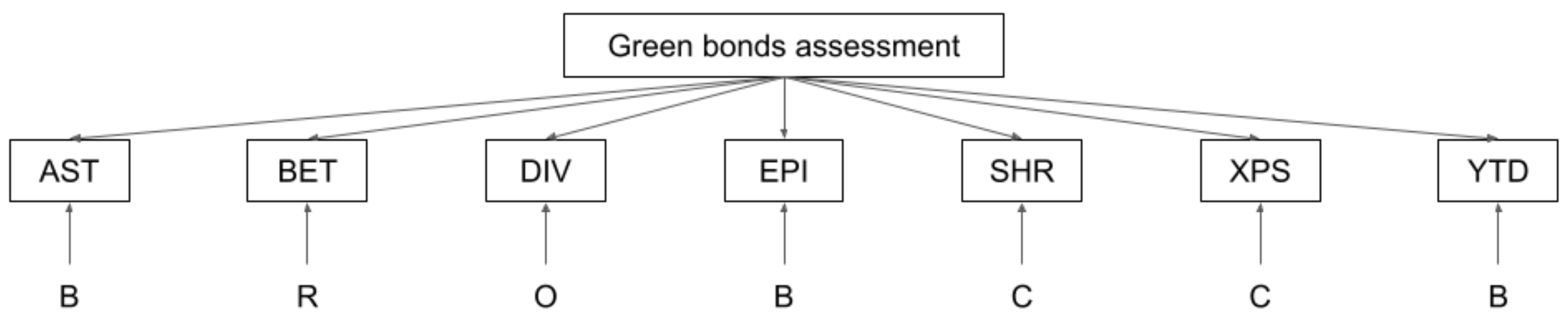
Figure 2 associates the set of criteria, proposed in this paper to assess green bonds, with the elements of BOCR Model. As it can be seen, all four elements of BOCR were considered in the set of criteria. Therefore, this is an exhaustive set of criteria, according to AHP Theory.

According to Figure 2, AST and EPI and YTD were criteria associated with benefits, id est, certain and favourable factors; DIV were associated with opportunities, i.e., uncertain favourable factors. Aligned with COPRAS Theory, all these four criteria may be considered as beneficial criteria. SHR and XPS were associated with costs, i.e., certain unfavourable factors, and BET is a risk, i.e., uncertain unfavourable factor. In addition, according to COPRAS, BET, SHR, and XPS are non-beneficial criteria.

As presented in Section 4, three experts on financial market provided data for weighting criteria in AHP, FUCOM, and SWARA:

• Expert 1 is a professional consultant with extensive experience in banking and international business consulting. He also acts as a lecturer for business and engineering colleges. As a PhD candidate, Expert 1 has the most scholar profile from the three experts. He was 49 years old in June 2021, when he provided data for this research.
• Expert 2 is a private investor, risk-taker levering investments in pursue for returns above market average. Recently graduated in a major course of industrial engineering, she moved her professional career to investment analysis already before her graduation. She was 25 years old in June 2021.
• Expert 3 is an investment fund manager, bearing a conservative position, accepting risks with caution, and pursuing safer returns. He has a bachelor degree in Economics and a Master in Business Administration. Expert 3 was 43 years old when he provided data for this research.

Therefore, there are three different positions from data provided by experts: Risk aversion (Expert 3), risk neutrality (Expert 1), and risk seeking (Expert 2). These positions results from their investor’s profiles: Aggressive (Expert 2), conservative (Expert 3), and moderate (Expert 1).

3.2. Analytic Hierarchy Process

AHP is a leading MCDA method [15] in diverse areas, such as chemical engineering, computer science, ecology, energy sector, health sector, higher education sector, manufacturing, mathematical advances, and supply chain management [47]. One important limitation of AHP is on the number of alternatives and criteria. Due the use of pairwise comparison matrices, a three-level hierarchy model must have no more than nine criteria or alternatives [48]. This limitation is one of the main reasons for a new trend in MCDA literature: hybrid-method application, mainly with AHP and TOPSIS [49]. This paper moves ahead this trend by combining AHP with COPRAS, FUCOM, and SWARA.

In AHP, weights for the criteria, usually named priorities, are obtained normalizing the right eigenvector $w=\left[w_j\right]$ of the pairwise comparison matrix $A=\left[a_{ij}\right]$, as in Equation (1), where ${\lambda }_{max}$ is its maximum eigenvalue.

$$Aw={\lambda }_{max}w$$

(1)

Usually, in AHP, the vector of weights $\widehat{w}=\left[\widehat{w_j}\right]$ is normalized from the eigenvector, as in Equation (2), for all $j=1,2\dots n$.

$$\widehat{w_j}=\frac{w_j}{{\sum }_{j=1}^n{w}_j}$$

(2)

Consistency checking is one of the great advantages of AHP against other MCDA methods. A consistent pairwise matrix A satisfies $a_{ij}=a_{ik}{a}_{kj}$, for all $i=1,2\dots n$, $j=1,2\dots n$, and $k=1,2\dots n$, resulting in ${\lambda }_{max}=n$, where n is the number of criteria. Consistency index $\mu$ is a measure of consistency of a pairwise matrix, as in Equation (2).

$$\mu =\frac{{\lambda }_{max}-n}{n-1}$$

(3)

Consistency ratio $CR$ is a better measure since it compares $\mu$ with a random index $RI$, computed by Oak Ridge Laboratory with more than 50,000 matrices [29], as in Equation (4).

$$CR=\frac{\mu }{RI}$$

(4)

Consistent matrices have ${\lambda }_{max}=n$, then $\mu =0$ and $CR=0$. Inconsistent matrices have at least one comparison, and its reciprocal, $a_{ij}\ne a_{ik}{a}_{kj}$, resulting in ${\lambda }_{max}>n$. It is desirable that $CR\le 0.1$, then A may be accepted, meaning “conformity with previous practice” [50], i.e., it means that experts did not change their minds, when fulfilling a pairwise comparison matrix.

3.3. Full Consistency Method

“Too many comparisons” is a frequent complaint expressed by AHP users [51]. For $n=7$ criteria, $n(n-1)/2=21$ comparisons are needed for a complete pairwise matrix. Incomplete pairwise comparisons (IPC) is an algorithm proposed to reduce the required number of comparisons for pairwise comparison matrices [52]. With IPC only $n=7$ comparisons will be needed. But, due to its complexity, IPC was, de facto, not applied in practice [53].

In the FUCOM Algorithm [31], only $n-1$ comparisons, generating a spanning tree [54], are required. The greatest advantage of FUCOM against IPC is its simplicity. However, FUCOM needs more interaction from the experts. At first, every expert need to rank the set of criteria, starting with the criterion that is expected to have the highest weight to the criterion of the least weight. For the ranked set of criteria $C=\{C_k,C_{k+1},C_{k+2}\dots C_{k+n}\}$, experts need to provide pairwise comparisons, named “comparative priority” ${\varphi }_{k/k+1}$. In this paper, Saaty Fundamental Scale [29], a linear 1–9 scale, will be used, for $a_{ij}$ in AHP, and for ${\varphi }_{k/k+1}$ in FUCOM, besides the use of this scale is not mandatory in FULCOM.

The weight of criteria $w_k$ in FUCOM must satisfy two conditions presented in Equations (5) and (6), for all $k=1,2\dots n$:

$$\frac{w_k}{w_{k+1}}={\varphi }_{k/k+1}$$

(5)

$$\frac{w_k}{w_{k+2}}=\left({\varphi }_{k/k+1}\right)\left({\varphi }_{(k+1)/(k+2)}\right)$$

(6)

Equation (6) results from mathematical transitivity $\frac{w_k}{w_{k+2}}=\frac{w_k}{w_{k+1}}\frac{w_{k+1}}{w_{k+2}}$. When both conditions are satisfied, the deviation for full consistency $\chi$ is minimum, i.e., $\chi =0$. The weights of criteria $w_k$ are obtained with Model (7), for all $k=1,2\dots n$:

$$\begin{array}{c}\hfill min\chi \\ \hfill \mathrm{subject}\mathrm{to}\\ \hfill |\frac{w_k}{w_{k+1}}-{\varphi }_{k/k+1}|\le \chi \\ \hfill |\frac{w_k}{w_{k+2}}-\left({\varphi }_{k/k+1}\right)\left({\varphi }_{(k+1)/(k+2)}\right)|\le \chi \\ \hfill \sum _{k=1}^n{w}_k=1\\ \hfill w_k\ge 0\end{array}$$

(7)

3.4. Step-Wise Weighting Assessment Ratio Analysis

SWARA has some similarities with FUCOM, despite having been developed earlier [17]. For instance, at first, the set of criteria needs to be ranked, from most important to the least. Then, criteria must be pairwise compared, but, as in FUCOM, only $n-1$ comparisons are needed. The first fundamental difference with SWARA is that Saaty Fundamental Scale is not adopted for the pairwise comparisons. Comparisons $s_k$ are the relative importance, i.e., how much one criterion is more important than another, in percentage, expressed in the $[0,1]$ interval. Comparison $s_1$ is between $C_1$ and $C_2$, $s_2$ is between $C_2$ and $C_3$... and $s_{n-1}$ is between $C_{n-1}$ and $C_n$.

In the next step, coefficients ${\kappa }_k$ are obtained for the criteria, as in Equation (8), for all $k=1,2\dots n$.

$${\kappa }_k=\{\begin{array}{ccc}\hfill 1& \hfill & \hfill \mathrm{if}k=1\\ \hfill 1+s_k& \hfill & \hfill \mathrm{if}k>1\end{array}$$

(8)

Initial weights $q_k$ are obtained for the criteria, as in Equation (9), for all $k=1,2\dots n$.

$$q_k=\{\begin{array}{ccc}\hfill 1& \hfill & \hfill \mathrm{if}k=1\\ \hfill q_{k-1}/{\kappa }_k& \hfill & \hfill \mathrm{if}k\ge 1\end{array}$$

(9)

Final weights $w_k$ are obtained for the criteria, as in Equation (10), for all $k=1,2\dots n$.

$$w_k=\frac{q_k}{{\sum }_{j=1}^n{q}_k}$$

(10)

3.5. Complex Proportional Assessment

There are available data for green bonds performance on all criteria presented in Section 3.1. However, these performances are measured in different units as US dollars, for AST, SHR, and YTD, or percentages for EPI and XPS, and even with ratios for BET and DIV. Different measures cannot be summed. They can be barely compared, at first glance. Perhaps, they can be subjectively compared by an expert after seeing them again, twice or more.

MCDA provides an objective way to operate and work with these measures. This is done with the major tool of multi-attribute analysis: The decision matrix $X=\left[x_{ij}\right]$, composed by performances of alternatives i regarding the criteria j, with $i=1,2\dots m$ and $j=1,2\dots n$.

In COPRAS, X must be firstly normalized to $R=\left[r_{ij}\right]$, as in Equation (11), for all $i=1,2\dots m$ and $j=1,2\dots n$.

$$r_{ij}=\frac{x_{ij}}{{\sum }_{j=1}^n{x}_{ij}}$$

(11)

Then, the normalized decision matrix R must be weighted to $D=\left[d_{ij}\right]$, as in Equation (12), where $w_j$ are the weights of criteria, for all $i=1,2\dots m$ and $j=1,2\dots n$.

$$d_{ij}=r_{ij}{w}_j$$

(12)

Criteria must be identified as “beneficial” or “non-beneficial” [36]. Then, for every Alternative i weighted normalized performances must be summed for beneficial, $s^{+}$, and non-beneficial criteria, $s^{-}$, as in Equations (13) and (14), for all $i=1,2\dots m$:

$$s_i^{+}=\sum _{j=1}^n{d}_{ij}\mathrm{for}\mathrm{beneficial}\mathrm{criteria}$$

(13)

$$s_i^{-}=\sum _{j=1}^n{d}_{ij}\mathrm{for}\mathrm{non}-\mathrm{beneficial}\mathrm{criteria}$$

(14)

Then, the significance of alternative i, $q_i$, is obtained with Equation (15), for $i=1,2\dots m$.

$$q_i=s_i^{+}+\frac{min\left(s_i^{-}\right){\sum }_{i=1}^m{s}_i^{-}}{s_i^{-}{\sum }_{i=1}^m\frac{min\left(s_i^{-}\right)}{s_i^{-}}}$$

(15)

Finally, relative utility of Alternative i, $u_i$, is obtained with Equation (16), for $i=1,2,3\dots m$.

$$u_i=\frac{q_i}{max\left(q_i\right)}$$

(16)

Despite the same name, U is not the linear utility function, as in Multi-Attribute Utility Theory [30]. Eventually, a COPRAS application may result alternatives without zero utilities and even negative utilities. Alternative i with the highest utility, $u_i=1$, is the best one.

3.6. Technique of Order Preference by Similarity to Ideal Solution

The first step to assess alternatives with TOPSIS is also a normalization of decision matrix X. Among several normalization procedures proposed in TOPSIS Theory, the max-min linear procedure was adopted in this research, due the consistency of this procedure. A case study on Turkish financial market [55] qualified this normalization procedure as reliable for TOPSIS, according to four conditions: (i) similar statistical distribution properties, (ii) similar identification of best and poor performers, (iii) similar ranking of alternatives, and (iv) equivalent performance scores. Furthermore, the consistency of the max-min linear normalization in TOPSIS was confirmed by other studies [56,57].

Equations (17) and (18) present the max-min linear normalization procedure of $V=\left[v_{ij}\right]$, for all $i=1,2\dots m$ and $j=1,2\dots n$:

$$v_{ij}=\frac{x_{ij}}{max\left(x_{ij}\right)}$$

(17)

Equation (17) is applicable for criteria to be maximized, i.e., the “beneficial” criteria, in COPRAS. For criteria to be minimized, or the “non-beneficial”, Equation (18) must be applied, for all $i=1,2\dots m$ and $j=1,2\dots n$.

$$v_{ij}=\frac{min\left(x_{ij}\right)}{x_{ij}}$$

(18)

A special case for Equation (18) occurs when $min\left(x_{ij}\right)=0$. In this case, $v_{ij}=1$, for $x_{ij}=min\left(x_{ij}\right)$, and $v_{ij}=0$, for all other $x_{ij}$. Then, $v_{ij}$ becomes a binary variable for this j.

In the next step, the normalized decision matrix V needs to be weighted by criteria weights w, resulting in $Y=\left[y_{ij}\right]$, as in Equation (19), for all $i=1,2\dots m$ and $j=1,2\dots n$.

$$y_{ij}=v_{ij}{w}_j$$

(19)

Besides the TOPSIS name refers to ideal solution, this method also works with the anti-ideal solution, also referred as negative ideal solution. Positive ideal solution $a^{+}$, and negative ideal solution $a^{-}$ can be obtained as in Equations (20) and (21), for all $i=1,2\dots m$ and $j=1,2\dots m$.

$$a_j^{+}=max\left(y_{ij}\right)$$

(20)

$$a_j^{-}=max\left(y_{ij}\right)$$

(21)

Then, Euclidean distances to negative ideal solution $d^{-}=\left[d_i^{-}\right]$ and to positive ideal solution $d^{+}=\left[d_i^{+}\right]+$ are obtained with Equations (22) and (23), for all $i=1,2\dots n$.

$$d_i^{-}=\sqrt{\sum _{j=1}^n{(y_{ij}-a_j^{-})}^2}$$

(22)

$$d_i^{-}=\sqrt{\sum _{j=1}^n{(y_{ij}-a_j^{-})}^2}$$

(23)

Finally, closeness coefficients $c_i$ are obtained, as in Equation (24), for all $i=1,2\dots n$.

$$c_i^{-}=\frac{d_i^{-}}{d_i^{-}+d_i^{+}}$$

(24)

When weighted performances $y_{ij}$ of alternatives i are closer to $a^{+}$ than $a^{-}$, then $c_i\ge 0.5$.

4. Results

4.1. Criteria Weighting

4.1.1. AHP Application

Table 3. Pairwise comparison matrix and normalized weights of criteria from Expert 1 (AHP).

Criterion	AST	BET	DIV	EPI	SHR	XPS	YTD	Weight
Assets (AST)	1	1/3	1	7	3	3	1	17.1%
Risk (BET)	3	1	1	7	1	5	1/3	18.4%
Dividend Yield (DIV)	1	1	1	9	3	3	1	20.7%
Country’s EPI	1/7	1/7	1/9	1	1/5	1/5	1/9	2.1%
Share (SHR)	1/3	1	1/3	5	1	3	1/3	10.2%
Expenses (XPS)	1/3	1/5	1/3	5	1/3	1	1/5	5.5%
Returns (YTD)	1	3	1	9	3	5	1	26.1%

presents a pairwise comparison matrix $A^1$ and the normalized weights of criteria ${\widehat{w}}^1$. Superscript 1 indicates that comparisons were provided by Expert 1. As presented in Section 3.1, Expert 1 has moderate profile for investing, and risk neutral position. The consistency ratio, $C{R}^1\approx 0.077$ indicates that $A^1$ can be accepted.

Table 4. Weights of criteria with AHP.

Criterion	Expert 1	Expert 2	Expert 3
AST	17.1%	14.8%	3.8%
BET	18.4%	1.7%	22.1%
DIV	20.7%	20.2%	25.6%
EPI	2.1%	3.1%	12.4%
SHR	10.2%	7.3%	1.7%
XPS	5.5%	12.5%	4.6%
YTD	26.1%	40.4%	29.8%

presents weights of criteria for Experts 1, 2, and 3. Weights from Experts 2 and 3 resulted from consistent comparison matrices, respectively, with $C{R}^2\approx 0.098$ and $C{R}^3\approx 0.097$.

Dividend yield (DIV) and returns to-date (YTD) are the top-two criteria for all experts. This was expected, since Experts 1, 2, and 3 have expertise as investors in traditional bonds markets. Expert 3 is a conservative investor, with risk aversion. Then, Risks (BET) is the third criteria for this expert. BET’s weight is higher for Expert 3 than for other experts, because Expert 3 considers more the impact of risks for bonds selections than Experts 1 and 2. Conversely, BET is the bottom-one criteria for Expert 2, which is an aggressive risk-taker investor. For Expert 2, YTD has more than 40% of weight. Again, very expected result, since this is an aggressive investor, seeking for returns.

EPI, the only non-financial criterion, had a low weight for Experts 1 and 3. EPI had the lowest weight for both aggressive investor, Expert 2, and for the moderate neutral-to-risk Expert 1. On the other hand, for the conservative investor, Expert 3, EPI has the third highest weight.

4.1.2. FUCOM Application

For Expert 1, the ranked set of criteria is $C^1=\{YTD,DIV,BET,AST,SHR,XPS,$$EPI\}$. As in AHP, superscript 1 indicates data collected from Expert 1.

Table 5. Pairwise comparisons and weights of criteria from Expert 1 (FUCOM).

Criterion	YTD	DIV	BET	AST	SHR	XPS	EPI	Raw Weight	Normal. Weight
YTD	1	1						1	28.7%
DIV		1	1					1	28.7%
BET			1	3				1	28.7%
AST				1	3			1/3	9.6%
SHR					1	3		1/9	3.2%
XPS						1	5	1/27	1.1%
EPI							1	1/135	0.2%

presents $n-1$ pairwise comparisons $\varphi$ between Criterion k and Criterion $k+1$, for $k=1,2\dots 6$, and their resulting weights, in raw and normalized.

Table 6. Weights of criteria with FUCOM.

Criterion	Expert 1	Expert 2	Expert 3
AST	9.6%	16.0%	3.8%
BET	28.7%	0.7%	11.5%
DIV	28.7%	16.0%	34.5%
EPI	0.2%	0.6%	3.8%
SHR	3.2%	3.2%	11.5%
XPS	1.1%	16.0%	0.4%
YTD	28.7%	48.0%	34.5%

presents weights of criteria from Experts 1, 2, and 3. Criteria set from Experts 2 and 3 were $C^2=${YTD, DIV, AST, XPS, SHR, EPI, BET} and $C^3=${YTD, DIV, BET, EPI, XPS, AST, SHR}.

Dividend yield (DIV) and returns to-date (YTD) are the top-two criteria for all experts, also with FUCOM, as with AHP. However, for Expert 1, Risks (BET) were tied-first with DIV and YTD. FUCOM application results tied weights from all experts. For Expert 2 Assets (AST) and Expenses (XPS) tied-second with DIV. Surprisingly, for Expert 3, BET tied-third with Share (SHR). More surprisingly, BET’s weight was higher for moderate investor Expert 2 than for conservative investor Expert 1. Experts were consulted about the result, confirming their comparison and expressing some understanding on results: “I do care about risk, but risks are not everything”, said Expert 3.

4.1.3. SWARA Application

After AHP and FUCOM applications, experts were asked to compared again the set of criteria, but not with Saaty Scale.

Table 7. Pairwise comparisons and weights of criteria from Expert 1 (SWARA).

Criterion	YTD	DIV	BET	AST	SHR	XPS	EPI	Raw Weight	Normal. Weight
YTD	1	0.25						1	26.4%
DIV		1	0.15					0.800	21.2%
BET			1	0.10				0.696	18.4%
AST				1	0.70			0.632	16.7%
SHR					1	0.85		0.372	9.8%
XPS						1	1.50	0.201	5.3%
EPI							1	0.080	2.1%

presents $n-1$ relative importance $s^1$ of Criterion k over Criterion $k+1$, according to Expert 1, for $k=1,2\dots 6$, and their resulting weights, in raw and normalized.

Table 8. Weights of criteria with SWARA.

Criterion	Expert 1	Expert 2	Expert 3
AST	16.7%	15.5%	5.5%
BET	18.4%	2.4%	20.9%
DIV	21.2%	20.9%	24.1%
EPI	2.1%	4.3%	12.0%
SHR	9.8%	7.6%	3.1%
XPS	5.3%	12.9%	6.8%
YTD	26.4%	36.5%	27.7%

presents weights of criteria from Experts 1, 2, and 3.

As for AHP and FUCOM, Dividend yield (DIV) and Returns to-date (YTD) are the top-two criteria for all experts, also with SWARA. Other results with SWARA are very close, or almost the same with the ones with AHP. Despite SWARA required less comparisons than AHP, and the same ones asked to experts for FUCOM, AHP’s and SWARA’s results are very much closer than FUCOM’s and SWARA’s.

4.2. Alternatives Assessment

4.2.1. COPRAS Application

Table 9. Decision matrix.

Bond	AST [USD]	BET	DIV	EPI	SHR [USD]	XPS	YTD [USD]
1	13,200,000,000	1.03	1.05	69.3	40.97	0.14%	12.02
2	478,000,000	0.90	0.93	69.3	98.22	0.49%	5.51
3	27,610,000,000	0.86	0.40	69.3	60.70	0.84%	13.23
4	7,880,000,000	0.95	0.18	69.3	44.02	0.98%	7.95
5	16,500,000,000	1.20	1.20	69.3	95.23	0.15%	13.05
6	7,300,000,000	1.20	1.30	69.3	44.90	0.25%	6.38
7	5,400,000,000	1.20	1.60	69.3	79.21	0.20%	8.68
8	5,500,000,000	1.20	0.40	69.3	23.24	0.46%	−19.17
9	1,100,000,000	0.99	1.20	69.3	104.77	0.20%	12.85
10	870,000,000	0.99	0.95	81.3	33.06	0.78%	5.00
11	917,000,000	0.96	1.25	69.3	37.49	0.35%	16.03
12	834,000,000	0.00	0.50	69.3	44.00	0.40%	5.00
13	6,600,000,000	1.13	1.53	69.3	10.55	0.64%	5.00
14	783,000,000	1.57	2.02	69.3	27.63	0.18%	−1.71
15	193,000,000	1.01	0.70	69.3	23.67	0.10%	5.00

presents the decision matrix X. Data were collected from https://epi.yale.edu (accessed on 17 September 2021) and https://www.kiplinger.com (accessed on 17 September 2021). Bonds names were suppressed for confidentiality reasons. After all, despite their data, including their names, are public data, this paper is not intended to advertise or to promote individual green bonds.

Table 10. Normalized decision matrix for COPRAS.

Bond	AST	BET	DIV	EPI	SHR	XPS	YTD
1	0.139	0.068	0.069	0.066	0.053	0.020	0.127
2	0.005	0.059	0.061	0.066	0.0128	0.069	0.058
3	0.290	0.057	0.026	0.066	0.079	0.119	0.140
4	0.083	0.063	0.012	0.066	0.057	0.139	0.084
5	0.173	0.079	0.079	0.066	0.124	0.021	0.138
6	0.077	0.079	0.086	0.066	0.058	0.035	0.067
7	0.057	0.079	0.105	0.066	0.103	0.028	0.092
8	0.058	0.079	0.026	0.066	0.030	0.065	−0.202
9	0.012	0.065	0.077	0.066	0.136	0.028	0.136
10	0.009	0.065	0.063	0.077	0.043	0.110	0.053
11	0.010	0.063	0.082	0.066	0.049	0.050	0.169
12	0.009	0.000	0.033	0.066	0.057	0.057	0.053
13	0.069	0.074	0.101	0.066	0.014	0.091	0.053
14	0.008	0.103	0.133	0.066	0.036	0.025	−0.018
15	0.002	0.066	0.046	0.066	0.031	0.142	0.053

presents the normalized decision matrix R, obtained from X, as in Equation (11).

Table 11. Normalized weighted decision matrix with Expert 1’s AHP weights for COPRAS.

Bond	AST	BET	DIV	EPI	SHR	XPS	YTD
1	0.02377	0.01251	0.01428	0.00139	0.00541	0.00110	0.03315
2	0.00086	0.01086	0.01263	0.00139	0.01306	0.00380	0.01514
3	0.04959	0.01049	0.00538	0.00139	0.00806	0.00655	0.03654
4	0.01419	0.01159	0.00248	0.00139	0.00581	0.00765	0.02192
5	0.02958	0.01454	0.01635	0.00139	0.01265	0.00116	0.03602
6	0.01317	0.01454	0.01780	0.00139	0.00592	0.00193	0.01749
7	0.00975	0.01454	0.02174	0.00139	0.01051	0.00154	0.02401
8	0.00992	0.01454	0.00538	0.00139	0.00306	0.00358	−0.05272
9	0.00205	0.01196	0.01594	0.00139	0.01387	0.00154	0.03550
10	0.00154	0.01196	0.01304	0.00162	0.00439	0.00605	0.01383
11	0.00171	0.01159	0.01697	0.00139	0.00500	0.00275	0.04411
12	0.00154	0.00000	0.00683	0.00139	0.00581	0.00314	0.01383
13	0.01180	0.01362	0.02091	0.00139	0.00143	0.00501	0.01383
14	0.00137	0.01895	0.02753	0.00139	0.00367	0.00138	−0.00470
15	0.00034	0.01214	0.00952	0.00139	0.00316	0.00781	0.01383

presents the normalized weighted decision matrix D, obtained with R multiplied by weights from Expert 1 for AHP $w^1$, as in Equation (12).

Assets (AST), Dividend Yield (DIV), Country’s EPI, and Returns (YTD) were considered as beneficial criteria. Conversely, Expenses (XPS), Risks (BET), and Share (SHR) were considered as non-beneficial criteria.

Table 12. Results with COPRAS application.

		AHP			FUCOM			SWARA
Bond	${\mathit{u}}^1$	${\mathit{u}}^2$	${\mathit{u}}^3$	${\mathit{u}}^1$	${\mathit{u}}^2$	${\mathit{u}}^3$	${\mathit{u}}^1$	${\mathit{u}}^2$	${\mathit{u}}^3$
1	1	0.956	0.813	1	0.992	1	1	1	1
2	0.306	0.412	0.533	0.412	0.331	0.489	0.320	0.352	0.438
3	0.949	1	0.776	0.894	1	0.789	0.948	0.963	0.775
4	0.408	0.509	0.495	0.424	0.475	0.433	0.412	0.454	0.438
5	0.847	0.982	0.850	0.929	0.907	0.933	0.866	0.898	0.843
6	0.510	0.649	0.636	0.600	0.500	0.644	0.515	0.528	0.584
7	0.582	0.719	0.738	0.729	0.593	0.800	0.588	0.620	0.697
8	−0.367	−0.456	−0.336	−0.529	−0.703	−0.644	−0.392	−0.546	−0.506
9	0.561	0.754	0.804	0.741	0.678	0.856	0.577	0.657	0.742
10	0.306	0.421	0.533	0.400	0.314	0.478	0.309	0.343	0.449
11	0.653	0.904	0.907	0.859	0.814	1	0.670	0.769	0.854
12	0.245	0.404	1	0.306	0.280	0.367	0.247	0.287	0.360
13	0.490	0.579	0.626	0.600	0.449	0.644	0.495	0.500	0.573
14	0.265	0.386	0.467	0.400	0.119	0.478	0.268	0.231	0.404
15	0.255	0.570	0.514	0.341	0.288	0.411	0.268	0.296	0.382

presents the relative utilities $u_i^e$ for green bonds i, according to Experts e, for all $e=1,2,3$ and $i=1,2\dots 15$.

4.2.2. TOPSIS Application

Table 13. Normalized decision matrix for TOPSIS.

Bond	AST	BET	DIV	EPI	SHR	XPS	YTD
1	0.478	0	0.520	0.852	0.075	0.714	0.750
2	0.017	0	0.460	0.852	0.031	0.204	0.344
3	1	0	0.198	0.852	0.050	0.119	0.825
4	0.285	0	0.089	0.852	0.070	0.102	0.496
5	0.598	0	0.594	0.852	0.032	0.667	0.814
6	0.264	0	0.644	0.852	0.068	0.400	0.398
7	0.196	0	0.792	0.852	0.039	0.500	0.536
8	0.199	0	0.201	0.852	0.944	0.217	−1.196
9	0.040	0	0.594	0.852	0.029	0.500	0.802
10	0.032	0	0.470	1	1	0.128	0.312
11	0.033	0	0.619	0.852	0.082	0.286	1
12	0.030	1	0.248	0.852	0.070	0.250	0.312
13	0.239	0	0.757	0.852	0.290	0.156	0.312
14	0.028	0	1	0.852	0.111	0.556	−0.107
15	0.007	0	0.347	0.852	0.129	1	0.312

presents the normalized decision matrix V, obtained from X, as in Equation (17) (applied for AST, DIV, EPI, and YTD) and Equation (18) (applied for BET, SHR, and XPS).

Table 14. Normalized weighted decision matrix with Expert 1’s AHP weights for TOPSIS.

Bond	AST	BET	DIV	EPI	SHR	XPS	YTD
1	0.0817	0	0.1076	0.0179	0.008	0.039	0.196
2	0.003	0	0.095	0.018	0.003	0.011	0.090
3	0.171	0	0.041	0.018	0.005	0.007	0.215
4	0.049	0	0.018	0.018	0.007	0.006	0.130
5	0.102	0	0.123	0.018	0.003	0.037	0.212
6	0.045	0	0.133	0.018	0.007	0.022	0.104
7	0.034	0	0.163	0.018	0.004	0.027	0.140
8	0.034	0	0.042	0.018	0.096	0.012	−0.312
9	0.007	0	0.123	0.018	0.003	0.028	0.209
10	0.006	0	0.097	0.021	0.102	0.007	0.081
11	0.006	0	0.128	0.018	0.008	0.016	0.261
12	0.005	0.184	0.051	0.018	0.007	0.014	0.081
13	0.041	0	0.157	0.018	0.030	0.009	0.081
14	0.005	0	0.207	0.018	0.011	0.031	−0.028
15	0.001	0	0.072	0.018	0.013	0.055	0.081
$a+$	0.171	0.184	0.207	0.021	0.102	0.055	0.261
$a-$	0.001	0	0.018	0.018	0.003	0.006	−0.312

presents the normalized weighted decision matrix Y, obtained with R multiplied by weights from Expert 1 for AHP $w^1$, as in Equation (19). Negative ideal solution $a^{-}$ and positive ideal solution $a^{+}$ are also presented.

Table 15. Results with TOPSIS application.

		AHP			FUCOM			SWARA
Bond	${\mathit{c}}^1$	${\mathit{c}}^2$	${\mathit{c}}^3$	${\mathit{c}}^1$	${\mathit{c}}^2$	${\mathit{c}}^3$	${\mathit{c}}^1$	${\mathit{c}}^2$	${\mathit{c}}^3$
1	0.672	0.817	0.690	0.634	0.844	0.738	0.675	0.802	0.685
2	0.281	0.332	0.363	0.297	0.323	0.374	0.285	0.332	0.361
3	0.497	0.618	0.467	0.416	0.662	0.467	0.496	0.595	0.465
4	0.245	0.294	0.308	0.244	0.294	0.242	0.246	0.291	0.308
5	0.517	0.702	0.535	0.466	0.743	0.580	0.520	0.684	0.534
6	0.319	0.355	0.383	0.324	0.331	0.366	0.322	0.364	0.385
7	0.433	0.524	0.504	0.453	0.515	0.567	0.439	0.523	0.501
8	0.355	0.375	0.361	0.345	0.380	0.366	0.354	0.371	0.360
9	0.451	0.607	0.532	0.461	0.629	0.588	0.457	0.586	0.526
10	0.460	0.658	0.524	0.458	0.707	0.602	0.464	0.619	0.501
11	0.509	0.678	0.585	0.512	0.703	0.655	0.515	0.650	0.575
12	0.350	0.168	0.427	0.412	0.129	0.260	0.350	0.189	0.428
13	0.368	0.376	0.431	0.397	0.335	0.482	0.373	0.388	0.429
14	0.334	0.321	0.389	0.363	0.292	0.417	0.338	0.336	0.392
15	0.238	0.293	0.314	0.250	0.292	0.262	0.238	0.312	0.326

presents the closeness coefficients $c_i^e$ for green bonds i, according to Experts e, for all $e=1,2,3$ and $i=1,2\dots 15$.

5. Discussion

Table 16. Ranks with MCDA methods applications according to Expert 1.

	AHP	AHP	FUCOM	FUCOM	SWARA	SWARA
Bond	COPRAS	TOPSIS	COPRAS	TOPSIS	COPRAS	TOPSIS
1	1	1	2	1	1	1
2	10	13	10	13	10	13
3	2	4	1	7	2	4
4	9	14	8	15	9	14
5	3	2	3	3	3	2
6	7	12	7	12	7	12
7	5	7	6	6	5	7
8	15	9	15	11	15	9
9	6	6	5	4	6	6
10	10	5	11	5	11	5
11	4	3	4	2	4	3
12	14	10	13	8	14	10
13	8	8	9	9	8	8
14	12	11	14	10	12	11
15	13	15	12	14	12	15

presents ranks of Kiplinger’s top-fifteen green bonds with MCDA methods applications. The ranks resulted from criteria weights according to Expert 1, a moderate neutral-to-risk investor.

Bond 1, ranked first by Kiplinger, was also ranked first by Expert 1, with almost all methods. The only exception was with FUCOM–COPRAS application ranking Bond 1 in second. Bond 11 was the most up-ranked green bond, moving up to second, third, or fourth ranks, depending on the MCDA method applied. Bonds 3 and 5 have also better ranks with MCDA than in the original Kiplinger’s rank. On the other hand, Bonds 2, 4, and 8 were the most down-ranked green bonds. And, Bond 15 was in the bottom-ranks.

Ranks resulted from COPRAS applications were moderately correlated with original Kiplinger’s rank. Spearman’s rank correlation coefficient $r_s$ [58] varied from 0.55 to 0.59 for the three COPRAS applications. Ranks resulted with TOPSIS were not correlated with Kiplinger’s. For TOPSIS applications, $r_s$ varies from 0.13 to 0.28.

Table 17. Ranks with MCDA methods applications according to Expert 2.

	AHP	AHP	FUCOM	FUCOM	SWARA	SWARA
Bond	COPRAS	TOPSIS	COPRAS	TOPSIS	COPRAS	TOPSIS
1	3	1	2	1	1	1
2	12	11	10	11	10	12
3	1	5	1	5	2	5
4	10	13	8	12	9	14
5	2	2	3	2	3	2
6	7	10	7	10	7	10
7	6	7	6	7	6	7
8	15	9	15	8	15	9
9	5	6	5	6	5	6
10	11	4	11	3	11	4
11	4	3	4	4	4	3
12	13	15	13	15	13	15
13	8	8	9	9	8	8
14	14	12	14	14	14	11
15	9	14	12	13	12	13

and

Table 18. Ranks with MCDA methods applications according to Expert 3.

	AHP	AHP	FUCOM	FUCOM	SWARA	SWARA
Bond	COPRAS	TOPSIS	COPRAS	TOPSIS	COPRAS	TOPSIS
1	1	1	1	1	1	1
2	10	12	10	10	10	12
3	3	7	2	8	4	7
4	9	15	9	15	10	15
5	2	3	3	5	3	3
6	7	11	7	11	7	11
7	6	6	5	6	6	5
8	15	13	15	12	15	13
9	5	4	6	4	5	4
10	11	5	11	3	9	6
11	4	2	4	2	2	2
12	14	9	14	14	14	9
13	7	8	8	7	8	8
14	11	10	12	9	12	10
15	13	14	12	13	13	14

present more ranks of Kiplinger’s top-fifteen green bonds with MCDA methods applications. These ranks resulted from criteria weights according to Experts 2 and 3, respectively, an aggressive risk-taker investor and a conservative investor with risk aversion.

According to Expert 2’s criteria weights, Bond 1 was also top ranked. However, not so best as for Expert 1, Bond 1 was third ranked with AHP–COPRAS. Bonds 3 and 5 were also in the top. Bonds 2, 4 and 8 were also down ranked in Table 17. Expert 2’s criteria weights favoured Bond 15, no longer being the last bond with any MCDA method.

Despite more variable, ranks with Expert 2’s weights were more correlated with original Kiplinger’s rank. Ranks resulted with AHP–COPRAS were less correlated, with $r_s\approx 0.41$. All other ranks kept or increased their $r_s$. For instance, $r_s$ for FUCOM–TOPSIS’s rank increased from 0.13, according to Expert 1, to 0.45 according to Expert 2.

According to Expert 3’s criteria weights, Bond 1 was top ranked with all MCDA methods. Bonds 3 and 5 were also in the top. Bonds 2, 4 and 8 were also down ranked in Table 18. As for Expert 2’s criteria weights, Bond 15 was also favoured, not being the last bond with any MCDA method application.

Ranks with Expert 2’s weights had two patterns of correlation with original Kiplin-ger’s rank. Ranks resulted with COPRAS were more correlated, with $r_s$ from 0.48 to 0.55. Ranks resulted with TOPSIS had $r_s\approx 0.16$. Correlation with TOPSIS was deeply impacted by Bond 4 worst performance, due the poor performance of the bond in YTD.

In addition to differences in results, the paper showed differences in processes. Experts were unanimous in their preference for the pair of methods SWARA–COPRAS. Among them, only Expert 1 had previously applied MCDA methods, also in a Sustainability problem, but with AHP and TOPSIS [13]. In the case of evaluating green bonds, SWARA proved to be more efficient than AHP and more effective than FUCOM. After all, SWARA required only six comparisons against the 21 required by AHP. COPRAS application provided better discriminated performance of alternatives, regarding risks (BET), than TOPSIS did. Experts 1 and 2 clearly preferred criteria weights with AHP and SWARA.

6. Conclusions

This paper achieved its main objective presenting a hybrid MCDA assessment of green bonds, with applications of AHP, COPRAS, FUCOM, SWARA, and TOPSIS. Consistent pairwise comparison matrices were provided on the criteria, by three experts in financial market. Data were collected from specialized database as Kiplinger magazine and Yale University’s Center for Environmental Law & Policy.

As it could be expected, different ranks were obtained with different experts and different methods of MCDA. However, there is moderate positive correlation between some ranks. Outstandingly, all the ranks coincided in the pole position. Coincidence is an indication those ranks pointing for the same direction. Divergence was due to different ranking methodologies. Data collected from different experts was another source for diverging results. Despite their expertise in investment analysis, experts’ profiles differ on decision-making behavior regarding risks: from risk aversion to risk seeking, including risk neutrality. Considering objective and subjective positions from different decision-makers, results are not matter of validation, comparing to a “correct answer” [59].

The green bonds assessment with multi-method MCDA applications is the major novelty of this paper. Literature searches have not found an MCDA study in the promising field of green bonds. In addition to the unprecedented application of MCDA in this field, the paper innovated with the application of novel MCDA methods, in a hybrid way with traditional methods.

Future research directions include the extension of green bonds from other countries than the United Kingdom (Bond 10) and the United States of America (all other bonds. This was a major delimitation of this work. As a recommendation, when aiming bonds for another country, it is very important to contact experts on investment analysis from that country, or in markets where those bonds are traded.

Other MCDA methods may also include incorporating decision approaches as Delphi Method or Fuzzy Systems. Dependency and feedback among criteria could be incorporated to another model, with the ANP. In addition, techniques for group decision-making may be useful for aggregating data from experts.

Experts expressed their preference for newer methods, COPRAS and SWARA, over traditional MCDA methods, AHP and TOPSIS. However, this finding needs to be interpreted with caution, as this paper presents only one study. As a consequence, more cases are needed to confirm their opinion as a fact.

References

- Wendling, Z.A.; Emerson, J.W.; de Sherbinin, A.; Esty, D.C.; Hoving, K.; Ospina, C.D.; Murray, J.M.; Gunn, L.; Ferrato, M.; Schreck, M.; et al. 2020 Environmental Performance Index; Yale Center for Environmental Law & Policy: New Haven, CT, USA, 2020. [Google Scholar]
- Kara, S.E.; Ibrahim, M.D.; Daneshvar, S. Dual efficiency and productivity analysis of renewable energy alternatives of OECD countries. Sustainability 2021, 13, 7401. [Google Scholar] [CrossRef]
- Wood, T. Mapped: The greenest countries in the world. Visual Capitalist. Available online: https://www.visualcapitalist.com/greenest-countries-in-the-world (accessed on 9 June 2021).
- Carvalho, H.; Duarte, S.; Machado, V.C. Lean, agile, resilient and green: Divergences and synergies. Int. J. Lean Six Sigma 2011, 2, 151–179. [Google Scholar] [CrossRef]
- Zhu, Q.; Sarkis, J.; Lai, K. Confirmation of a measurement model for green supply chain management practices implementation. Int. J. Prod. Econ. 2008, 111, 261–273. [Google Scholar] [CrossRef]
- Pham, L. Is it risky to go green? A volatility analysis of the green bond market. J. Sustain. Financ. Invest. 2016, 6, 263–291. [Google Scholar] [CrossRef]
- Banga, J. The green bond market: A potential source of climate finance for developing countries. J. Sustain. Financ. Invest. 2019, 9, 17–32. [Google Scholar] [CrossRef]
- Environmental Finance. Available online: https://www.environmental-finance.com/content/the-green-bond-hub/environmental-finances-sustainable-bonds-insight-2021-introduction.html (accessed on 9 June 2021).
- Bloomberg Financial Services. Available online: https://www.bloomberg.com/professional/solution/sustainable-finance/ (accessed on 9 June 2021).
- S&P Global. Available online: https://www.spglobal.com/ratings/en/products-benefits/products/sustainable-finance-reviews-opinions (accessed on 9 June 2021).
- Vázquez-Rowe, I.; Córdova-Arias, C.; Brioso, X.; Santa-Cruz, S. A method to include life cycle assessment results in choosing by advantage (CBA) multicriteria decision analysis. A case study for seismic retrofit in Peruvian primary schools. Sustainability 2021, 13, 8139. [Google Scholar] [CrossRef]
- Zavadskas, E.K.; Turkis, Z.; Kildiene, S. State of art surveys of overviews on MCDM/MADM methods. Technol. Econ. Dev. Econ. 2014, 20, 165–179. [Google Scholar] [CrossRef] [Green Version]
- Lombardi Netto, A.; Salomon, V.A.P.; Ortiz-Barrios, M.A.; Florek-Paszkowska, A.K.; Petrillo, A.; De Oliveira, O.J. Multiple criteria assessment of sustainability programs in the textile industry. Int. Trans. Oper. Res. 2020, 28, 1550–1572. [Google Scholar] [CrossRef]
- Saaty, T.L.; Ergu, D. When a is a decision-making method trustworthy? Criteria for evaluating multi-criteria decision-making methods. Int. J. Inf. Technol. Dec. 2015, 14, 1171–1187. [Google Scholar] [CrossRef]
- Khan, S.A.; Chaabane, A.; Dweiri, F.T. Multi-criteria decision-making methods application in supply chain management: A systematic literature review. In Multi-Criteria Methods and Techniques Applied to Supply Chain Management; Salomon, V.A.P., Ed.; Intech Open: London, UK, 2018; pp. 3–31. [Google Scholar]
- Tramarico, C.L.; Mizuno, D.; Salomon, V.A.P.; Marins, F.A.S. Analytic hierarchy process and supply chain management: A bibliometric study. Procedia Comput. Sci. 2015, 55, 441–450. [Google Scholar] [CrossRef] [Green Version]
- Alinezhad, A.; Khalili, J. New Methods and Applications in Multiple Attribute Decision Making; Springer Nature: Cham, Switzerland, 2019. [Google Scholar]
- Ortiz-Barrios, M.; Cabarcas-Reyes, J.; Ishizaka, A.; Barbati, M.; Jaramillo-Rueda, N.; Carrascal-Zambrano, G.J. A hybrid fuzzy multi-criteria decision making model for selecting a sustainable supplier of forklift filters: A case study from the mining industry. Ann. Oper. Res. 2020. [Google Scholar] [CrossRef]
- Ortiz-Barrios, M.; Alfaro-Saiz, J.-J. A hybrid fuzzy multi-criteria decision-making model to evaluate the overall performance of public emergency departments: A case study. Int. J. Inf. Technol. Dec. 2020, 19, 1485–1548. [Google Scholar] [CrossRef]
- Kucera, J.; Vochozka, M.; Rowland, Z. The ideal debt ratio of an agricultural enterprise. Sustainability 2021, 13, 4613. [Google Scholar] [CrossRef]
- Zerbib, O.B. The effect of pro-environmental preferences on bond prices: Evidence from green bonds. J. Bank. Finance 2019, 98, 39–60. [Google Scholar] [CrossRef]
- Reboredo, J.C. Green bond and financial markets: Co-movement, diversification and price spillover effects. Energy Econ. 2018, 74, 38–50. [Google Scholar] [CrossRef]
- Tang, D.Y.; Zhang, Y. Do shareholders benefit from green bonds? J. Corp. Finance 2020, 61, 101427. [Google Scholar] [CrossRef]
- Febi, W.; Schäfer, D.; Stephan, A.; Sun, C. The impact of liquidity risk on the yield spread of green bonds. Financ. Res. Lett. 2018, 27, 53–59. [Google Scholar] [CrossRef]
- Hachenberg, B.; Schiereck, D. Are green bonds priced differently from conventional bonds? J. Assets Man. 2018, 19, 371–383. [Google Scholar] [CrossRef]
- Gianfrate, G.; Peri, M. The green advantage: Exploring the convenience of issuing green bonds. J. Clean. Prod. 2019, 219, 127–135. [Google Scholar] [CrossRef]
- Bachelet, M.J.; Becchetti, L.; Manfredonia, S. The green bonds premium puzzle: The role of issuer characteristics and third-party verification. Sustainability 2019, 11, 1098. [Google Scholar]
- Ng, T.H.; Tao, J.Y. Bond financing for renewable energy in Asia. Energy Policy 2016, 40, 509–517. [Google Scholar] [CrossRef] [Green Version]
- Saaty, T.L. The Analytic Hierarchy Process; McGraw-Hill: New York, NY, USA, 1980. [Google Scholar]
- Ishizaka, A.; Nemery, P. Multi-Criteria Decision Analysis; Wiley: Chichester, UK, 2018. [Google Scholar]
- Pamucar, D.; Stevic, Z.; Sremac, S. A new model for determining weight coefficients of criteria in MCDM Models: Full Consistency Method (FUCOM). Symmetry 2018, 10, 939. [Google Scholar] [CrossRef] [Green Version]
- Keršulienė, V.; Zavadskas, E.K.; Turskis, Z. Selection of rational dispute resolution method by applying new step-wise weight assessment ratio analysis (SWARA). J. Bus. Econ. Manag. 2010, 11, 243–258. [Google Scholar] [CrossRef]
- Zavadskas, E.K.; Kaklauskas, A.; Sarka, V. The new method of multicriteria complex proportional assessment of projects. Technol. Econ. Dev. Econ. 1994, 3, 131–139. [Google Scholar]
- Hwang, C.-L.; Yoon, K. Multiple Attribute Decision Making; Springer: New York, NY, USA, 1981. [Google Scholar]
- Zyoud, S.H.; Fuchs-Hanusch, D. A bibliometric-based survey on AHP and TOPSIS techniques. Expert Syst. Appl. 2017, 78, 158–181. [Google Scholar] [CrossRef]
- Mousavi-Nasab, S.H.; Sotoudeh-Anvari, A. A comprehensive MCDM-based approach using TOPSIS, COPRAS and DEA as an auxiliary tool for material selection problems. Mater. Des. 2017, 121, 237–253. [Google Scholar] [CrossRef]
- Pitchipoo, P.; Vincent, D.S.; Rajini, N.; Rajakarunakaran, S. COPRAS decision model to optimize blind spot in heavy vehicles: A comprehensive perspective. Procedia Eng. 2014, 97, 1049–1059. [Google Scholar] [CrossRef] [Green Version]
- Durmić, E. Evaluation of criteria for sustainable supplier selection using FUCOM method. ORESTA 2019, 2, 91–107. [Google Scholar] [CrossRef]
- Durmić, E.; Stević, Ž.; Chatterjee, P.; Vasiljević, M.; Tomašević, M. Sustainable supplier selection using combined FUCOM–Rough SAW model. Rep. Mech. Eng. 2020, 1, 34–43. [Google Scholar] [CrossRef]
- Hicks, C. 15 Best ESG Funds for Responsible Investors. Kiplinger. Available online: https://www.kiplinger.com/slideshow/investing/t041-s001-15-best-esg-funds-for-responsible-investors/index.html (accessed on 9 June 2021).
- Abraham, F.; Schmukler, S.; Tessada, J. Robo-advisors: Investing through machines. In World Bank Research and Policy Briefs; World Bank Group: Washington, DC, USA, 2019; Volume 134881, Available online: https://papers.ssrn.com/sol3/papers.cfm?abstract_id=3360125 (accessed on 9 June 2021).
- Coe, T.S.; Lasosethakul, K. Applying technical trading rules to beat long-term investing: Evidence from Asian market. Asia-Pac. Financ. Mark. 2021, 1–25. [Google Scholar] [CrossRef]
- Zhang, Y.; Rupp, J.A.; Graham, J.D. Contrasting public and scientific assessments of fracking. Sustainability 2021, 13, 6650. [Google Scholar] [CrossRef]
- Lee, C.-Y.; Chen, B.-S. Mutually-exclusive-and-collectively-exhaustive feature selection scheme. Appl. Soft Comput. 2018, 68, 961–971. [Google Scholar] [CrossRef]
- Mu, E.; Cooper, O.; Peasley, M. Best practices in analytic network process studies. Expert Syst. Appl. 2020, 159, 113536. [Google Scholar] [CrossRef]
- Shih, H.-S.; Cheng, C.-B.; Chen, C.-C.; Lin, Y.-C. Environmental impact on the vendor selection problem in electronics firms: A systematic analytic network process with BOCR. Int. J. AHP 2014, 6, 202–227. [Google Scholar] [CrossRef]
- Emrouznejad, A.; Marra, M. The state of the art development of AHP (1979–2017): A literature review with a social network analysis. Int. J. Prod. Res. 2017, 55, 6653–6675. [Google Scholar] [CrossRef] [Green Version]
- Salomon, V.A.P. Absolute measurement and ideal synthesis on AHP. Int. J. AHP 2016, 8, 538–545. [Google Scholar] [CrossRef]
- Ortiz-Barrios, M.; Miranda-De la Hoz, C.; López-Meza, P.; Petrillo, A.; De Felice, F. A case of food supply chain management with AHP, DEMATEL, and TOPSIS. J. MCDA 2019, 27, 104–128. [Google Scholar] [CrossRef]
- Saaty, T.L. Mathematical Principles of Decision-Making, Kindle ed.; RWS: Pittsburgh, PA, USA, 2013. [Google Scholar]
- Wedley, W.C. Fewer comparisons: Efficiency via sufficient redundancy. In Proceedings of the Tenth International Symposium on the Analytic Hierarchy Process, Pittsburgh, PA, USA, 29 July–1 August 2009; pp. 1–15. [Google Scholar]
- Harker, P.T. Incomplete pairwise comparisons in the analytic hierarchy process. Math. Model. 1987, 9, 837–848. [Google Scholar]
- Fedrizzi, M.; Giove, S. Incomplete pairwise comparison and consistency optimisation. Eur. J. Oper. Res. 2007, 183, 303–313. [Google Scholar] [CrossRef] [Green Version]
- Goodrich, M.T.; Tamassia, R. Algorithm Design; Wiley: New York, NY, USA, 2002. [Google Scholar]
- Çelen, A. Comparative analysis of normalization procedures in TOPSIS method: With an application to Turkish deposit banking market. Informatica 2014, 25, 185–208. [Google Scholar] [CrossRef] [Green Version]
- Shih, H.S.; Shyur, H.J.; Lee, E.S. An extension of TOPSIS for group decision making. Math. Model. 2007, 45, 801–813. [Google Scholar] [CrossRef]
- Bai, C.; Dhavale, D.; Sarkis, J. Integrating Fuzzy C-Means and TOPSIS for performance evaluation: An application and comparative analysis. Expert Syst. Appl. 2014, 41, 4186–4196. [Google Scholar] [CrossRef]
- Falk, R.; Well, A.D. Many faces of correlation coefficient. J. Stat. Educ. 1997, 5. [Google Scholar] [CrossRef]
- Whitaker, R. Validation examples of the analytic hierarchy process and analytic network process. Math. Model. 2007, 46, 840–859. [Google Scholar] [CrossRef]
Figure 1.
Research methodology.
Figure 2.
Set of criteria associated with BOCR Model.