
Pollution Accounting for Corporate Actions: Quantifying the Air Emissions and Impacts of Transportation System Choices Case Study: Food Freight and the Grocery Industry in Los Angeles


Abstract
:1. Executive Summary
2. Background
3. Purpose: Accounting for Air Pollution by Sector and Company
4. Top-Down Approach
4.1. Purpose and Intent
4.2. Method for Quantifying Total Emissions
- 1.
- Data Sources
- 2.
- Geographic Boundary Setting
- 3.
- Commodity Freight Flow Data
- 4.
- Distance Estimation
- 5.
- Calculating Emissions
- 6.
- Translating to monetary and health impacts
4.3. Method for Apportioning Emissions to Companies
- 1.
- Grocery industry and store share of food consumption
- 2.
- Corporate attribution
4.4. Analytical Demonstration of Top-Down Method
4.5. Results of Top-Down Approach Application
- 1.
- Food freight tonnage and ton-miles
- 2.
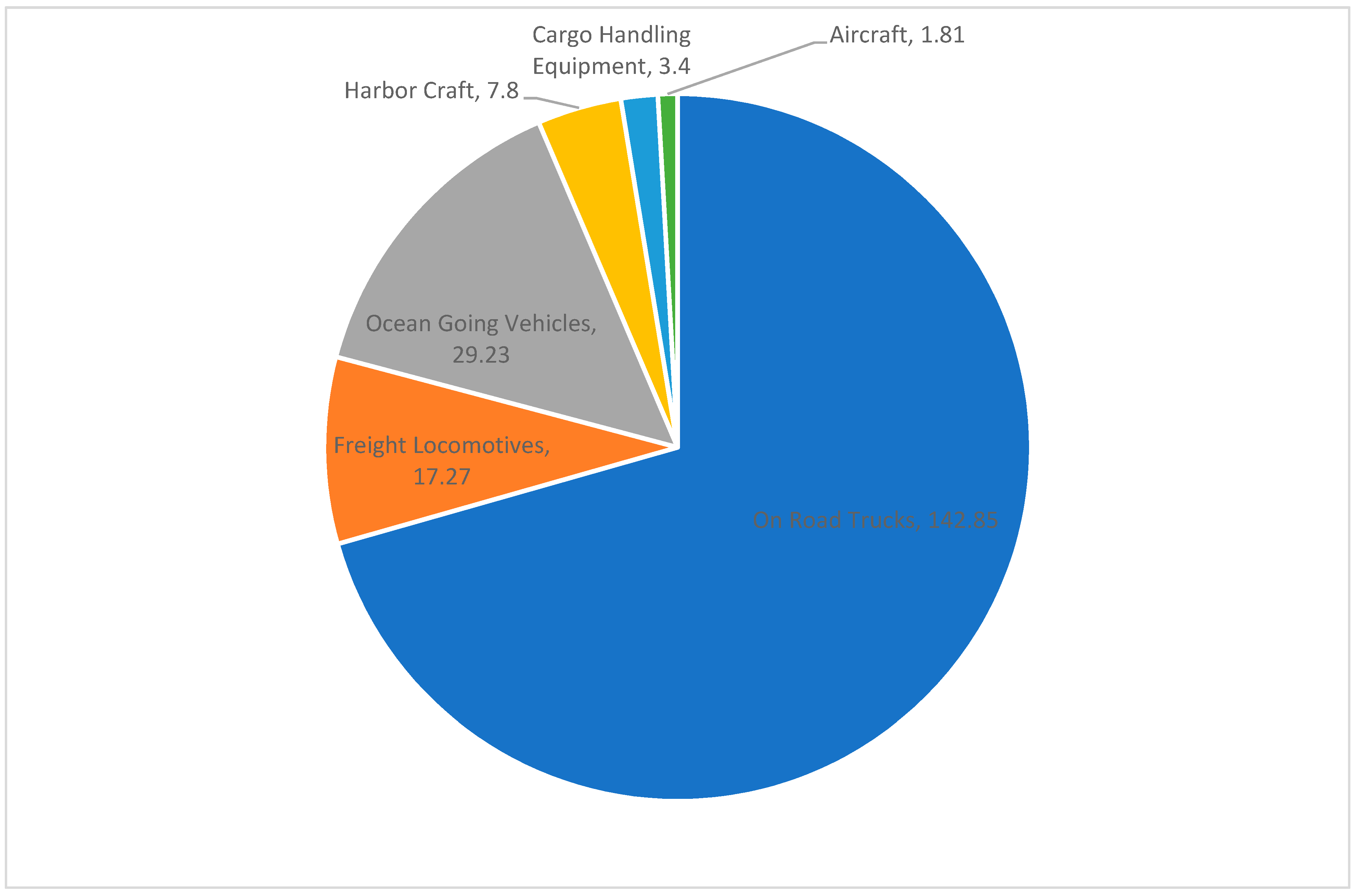
- Emissions impact
- 618,000 tons of CO2,
- 1549 tons of NOx and
- 24.6 tons of PM2.5.
- 3.
- Apportionment to individual companies
5. Bottom-Up Approach
5.1. Purpose and Intent
5.2. Method for Quantifying Corporate-Level Emissions
- 1.
- Distribution segment analytical framework
- Transport from a good’s first point of entry to first destination in region of interest
- Pickup and transport from manufacturing and processing centers
- Pickup and transport from distribution centers
- Drop off at retail/wholesale stores
- Final drop off at customer establishment after pick-up at retail/wholesale store
- 2.
- Scaling to single-truck-level emissions:
- 3.
- Scaling to corporation-level emissions:

- 4.
- Translating to monetary and health impacts
5.3. Areas of Uncertainty and Data Gaps
- 1.
- Distance travelled
- 2.
- Idling time
- 3.
- Emissions factors
- 4.
- Scaling
6. Results
6.1. Summary of Analytical Findings
- 1.
- Top-down method
- 2.
- Bottom-up method
6.2. Discussion: Further Areas of Analysis for Accuracy and Scaling
- First, a comprehensive analysis of goods movement emissions in the Los Angeles area that expands the top-down approach beyond the food sector and then compares observations with the findings of this paper.
- Second, a truck-level analysis that quantifies the air quality benefits from a single zero-emissions truck and the damages of a single diesel truck, depending on VMT and truck type.
- Third, community-level proximity mapping that highlights the disproportionate risk from goods movement emissions on communities of color and provides a detailed spatial assessment of where individual corporations can prioritize investments in local communities.
- Fourth, emissions analysis that evaluates the appropriateness of current emissions factors used for vehicles and ensures those factors accurately represent in-use truck emissions
- 1.
- Comprehensive Goods Movement Emissions Analysis
- 2.
- Truck-Level Analysis
- 3.
- Proximity Mapping
- 4.
- Emissions Factor Analysis
6.3. Relevance to Corporate Actors and Investors
6.4. Relevance to Academic Institutions and Researchers
7. Conclusions
Author Contributions
Funding
Institutional Review Board Statement
Data Availability Statement
Acknowledgments
Conflicts of Interest
Appendix A. Source Data Summary
Appendix A.1. SCAQMD Air Emissions Inventories


Appendix A.2. Multiple Air Toxics Exposure Study
Appendix A.3. AB617 Community Air Initiatives
Appendix A.4. Freight Analysis Framework
Appendix A.5. Corporate Sustainability Reporting
References
- Electrification Coalition. “Electrification Coalition Partners with Nestlé to Electrify Freight Route,” Electrification Coalition. 3 December 2020. Available online: https://www.electrificationcoalition.org/electrification-coalition-partners-with-nestle-to-electrify-freight-route/ (accessed on 8 September 2021).
- Cooper, C.; Sedgwick, S.; Mitra, S. Goods on the Move: Trade and Logistics in Southern California. Los Angeles County Economic Development Corporation (LAEDC). 2017. Available online: https://laedc.org/wp-content/uploads/2017/06/TL_20170515_Final.pdf (accessed on 8 September 2021).
- South Coast Air Quality Management District. Final 2016 Air Quality Management Plan. 2017. Available online: http://www.aqmd.gov/docs/default-source/clean-air-plans/air-quality-management-plans/2016-air-quality-management-plan/final-2016-aqmp/final2016aqmp.pdf?sfvrsn=15 (accessed on 8 September 2021).
- Reichmuth, D. Inequitable Exposure to Air Pollution from Vehicles in California; Union of Concerned Scientists: Cambridge, MA, USA, 2019; Available online: https://www.ucsusa.org/resources/inequitable-exposure-air-pollution-vehicles-california-2019 (accessed on 8 September 2021).
- Office of Environmental Health Hazard Assessment. California Communities Environmental Health Screening Tool, Version 3.0 (CalEnviroScreen 3.0): Guidance and Screening Tool; California Environmental Protection Agency: Sacramento, CA, USA, 2018.
- Tessum, W.; Paolella, D.A.; Chambliss, S.E.; Apte, J.S.; Hill, J.D.; Marshall, J.D. PM2.5 polluters disproportionately and systemically affect people of color in the United States. Sci. Adv. 2021, 7, eabf4491. Available online: https://advances.sciencemag.org/content/7/18/eabf4491 (accessed on 8 September 2021). [CrossRef] [PubMed]
- Coel, D.; Carlson, R. Goods Movement 2016 AQMP Whitepaper. 2015. Available online: http://www.aqmd.gov/docs/default-source/Agendas/aqmp/white-paper-working-groups/wp-goodsmvmt-final.pdf?sfvrsn=2 (accessed on 8 September 2021).
- South Coast Air Quality Management District. Multiple Air Toxics Exposure Study in the South Coast Air Basin. 2015. Available online: http://www.aqmd.gov/docs/default-source/air-quality/air-toxic-studies/mates-iv/mates-iv-final-draft-report-4-1-15.pdf (accessed on 8 September 2021).
- Southerland, V.A.; Anenberg, S.C.; Harris, M.; Apte, J.; Hystad, P.; van Donkelaar, A.; Martin, R.V.; Beyers, M.; Roy, A. Assessing the Distribution of Air Pollution Health Risks within Cities: A Neighborhood-Scale Analysis Leveraging High-Resolution Data Sets in the Bay Area, California. Environ. Health Perspect. 2021, 129, 037006. [Google Scholar] [CrossRef] [PubMed]
- Sinnamon, H. Accelerating to 100% Clean: Zero Emitting Vehicles Save Lives, Advance Justice, Create Jobs. Environmental Defense Fund. 2020. Available online: https://www.edf.org/sites/default/files/documents/TransportationWhitePaper.pdf (accessed on 8 September 2021).
- Mathers, J.; Craft, E.; Norsworthy, M.; Wolfe, C. The Green Freight Handbook. Environmental Defense Fund (EDF). 2019. Available online: https://supplychain.edf.org/resources/the-green-freight-handbook/ (accessed on 8 September 2021).
- Federal Highway Administration. Freight Analysis Framework. 2019. Available online: https://ops.fhwa.dot.gov/freight/freight_analysis/faf/index.htm (accessed on 8 September 2021).
- United States Census Bureau. Commodity Flow Survey (CFS). 2012. Available online: https://www.census.gov/programs-surveys/cfs.html (accessed on 8 September 2021).
- United States Census Bureau. SCTG Commodity Code List. 2020. Available online: https://bhs.econ.census.gov/bhsphpext/brdsearch/scs_code.html (accessed on 8 September 2021).
- Bureau of Transportation Statistics. 2012 CFS Public Use Microdata Visuals. Available online: https://www.bts.gov/content/cfs-areas (accessed on 8 September 2021).
- United States Environmental Protection Agency. 2020 SmartWay Truck Carrier Partner Tool: Truck Tool Technical Documentation. 2020. Available online: https://www.epa.gov/sites/production/files/2020-01/documents/420b20002.pdf (accessed on 8 September 2021).
- United States Environmental Protection Agency. SmartWay Carrier Performance Ranking. 2019. Available online: https://www.epa.gov/smartway/smartway-carrier-performance-ranking (accessed on 8 September 2021).
- Fann, N.; Chan, E. Technical Support Document: Estimating the Benefit per Ton of Reducing PM2.5 Precursors from 17 Sectors. U.S. Environmental Protection Agency. 2018. Available online: https://www.epa.gov/sites/production/files/2018-02/documents/sourceapportionmentbpttsd_2018.pdf (accessed on 8 September 2021).
- Lepeule, J.; Laden, F.; Dockery, D.; Schwartz, J. Chronic Exposure to Fine Particles and Mortality: An Extended Follow-up of the Harvard Six Cities Study from 1974 to 2009. Environ. Health Perspect. 2012, 120, 965–970. [Google Scholar] [CrossRef] [PubMed]
- United States Department of Agriculture: Economic Research Service. Food Service Industry: Market Segments. 2020. Available online: https://www.ers.usda.gov/topics/food-markets-prices/food-service-industry/market-segments/ (accessed on 8 September 2021).
- Saksena, M.J.; Okrent, A.M.; Anekwe, T.D.; Cho, C.; Dicken, C.; Effland, A.; Elitzak, H.; Guthrie, J.; Hamrick, K.S.; Hyman, J.; et al. America’s Eating Habits: Food Away From Home. United States Department of Agriculture Economic Research Service. 2018. Available online: https://www.ers.usda.gov/webdocs/publications/90228/eib-196.pdf (accessed on 8 September 2021).
- ACOSTA. COVID-19: Reinventing How America Eats. 10 September 2020. Available online: https://www.acosta.com/news/new-acosta-report-details-how-covid-19-is-reinventing-how-america-eats/ (accessed on 8 September 2020).
- Peltz, J.; Spacek, R. Southern California’s grocery battle heats up with the spread of discounter Aldi, Los Angeles Times. 27 June 2017. Available online: https://www.latimes.com/business/la-fi-agenda-grocery-wars-20170627-story.html (accessed on 8 September 2021).
- Gara, A. Sysco Cancels $8.2 Billion US Foods Takeover in Big Antitrust Win for FTC, Forbes. 29 June 2015. Available online: https://www.forbes.com/sites/antoinegara/2015/06/29/sysco-cancels-8-2-billion-us-foods-takeover-in-big-antitrust-win-for-ftc/?sh=56a429e742fc (accessed on 8 September 2021).
- Sysco. Sysco Reports Fourth Quarter and Full Year 2019 Results. 12 August 2019. Available online: https://investors.sysco.com/annual-reports-and-sec-filings/news-releases/2019/08-12-2019-130322864 (accessed on 8 September 2021).
- US Foods. US Foods Reports Fourth Quarter and Fiscal Year 2019 Earnings. 11 February 2020. Available online: https://ir.usfoods.com/investors/stock-information-news/press-release-details/2020/US-Foods-Reports-Fourth-Quarter-and-Fiscal-Year-2019-Earnings/default.aspx (accessed on 8 September 2021).
- Khan, M.; Komanduri, A.; Pacheco, K.; Ayvalik, C.; Proussaloglou, K.; Brogan, J.J.; McCourt, M.; Mak, R. Findings from the California Vehicle Inventory and Use Survey. J. Transp. Res. Board 2019, 1673, 349–360. [Google Scholar] [CrossRef]
- EPA. Technical Support Document Estimating the Benefit per Ton of Reducing PM2.5 Precursors from 17 Sectors U.S. Environmental Protection Agency Office of Air and Radiation Office of Air Quality Planning and Standards Research Triangle Park, NC 27711. February 2018. Available online: https://www.epa.gov/sites/default/files/2018-02/documents/sourceapportionmentbpttsd_2018.pdf (accessed on 8 September 2021).
- Gunders, D. Wasted: How America Is Losing Up to 40 Percent of Its Food from Farm to Fork to Landfill. NRDC Issue Paper. 2012. Available online: https://www.nrdc.org/sites/default/files/wasted-food-IP.pdf (accessed on 8 September 2021).
- Berry, T. On Average, How Much Do Stores Mark up Products? 2 December 2008. Available online: https://www.entrepreneur.com/answer/221767 (accessed on 8 September 2021).
- Khan, A.S.; Clark, N.N.; Gautam, M.; Wayne, W.S.; Thompson, G.J.; Lyon, D.W. Idle Emissions from Medium Heavy-Duty Diesel and Gasoline Trucks. J. Air Waste Manag. Assoc. 2009, 59, 354–359. [Google Scholar] [CrossRef] [PubMed]
- ICF. U.S. Freight GHG Emissions by Consuming Industry Segment. 2014. Available online: https://www.icf.com/ (accessed on 8 September 2021).
- South Coast Air Quality Management District, AB 617 Community Air Monitoring Plan (CAMP) for the San Bernardi-no/Muscoy Community. 2018. Available online: http://www.aqmd.gov/docs/default-source/ab-617-ab-134/camps/sbm_camp.pdf?sfvrsn=6 (accessed on 8 September 2021).
- South Coast Air Quality Management District. Final 2016 Air Quality Management Plan, Appendix 3: Base and Future Year Emission Inventory. Attachment A. 2020 Annual Average Emissions by Source Category in South Coast Air Basin. 2017. Available online: http://www.aqmd.gov/docs/default-source/clean-air-plans/air-quality-management-plans/2016-air-quality-management-plan/final-2016-aqmp/appendix-iii.pdf (accessed on 9 September 2021).
- EMFAC. “Emissions Inventory”, California Air Resources Board. 2020. Available online: https://arb.ca.gov/emfac/emissions-inventory (accessed on 8 September 2021).
- EMFAC2017 Volume III—Technical Documentation. California Air Resources Board. 2015. Available online: https://ww3.arb.ca.gov/msei/downloads/emfac2017-volume-iii-technical-documentation.pdf (accessed on 8 September 2021).
- EMFAC2014 Volume III—Technical Documentation. Available online: https://ww3.arb.ca.gov/msei/downloads/emfac2014/emfac2014-vol3-technical-documentation-052015.pdf (accessed on 8 September 2021).
- South Coast Air Quality Management District. Community Emissions Reduction Plan: Wilmington, Carson, West Long Beach. 2019. Available online: http://www.aqmd.gov/docs/default-source/ab-617-ab-134/steering-committees/wilmington/cerp/final-cerp-wcwlb.pdf?sfvrsn=8 (accessed on 8 September 2021).
- South Coast Air Quality Management District. Community Emissions Reduction Plan: East Los Angeles, Boyle Heights, West Commerce. 2019. Available online: http://www.aqmd.gov/docs/default-source/ab-617-ab-134/steering-committees/east-la/cerp/carb-submittal/final-cerp.pdf?sfvrsn=8 (accessed on 8 September 2021).
- South Coast Air Quality Management District. Community Emissions Reduction Plan: San Bernardino, Muscoy. 2019. Available online: http://www.aqmd.gov/docs/default-source/ab-617-ab-134/steering-committees/san-bernardino/cerp/carb-submittal/final-cerp.pdf?sfvrsn=9 (accessed on 8 September 2021).


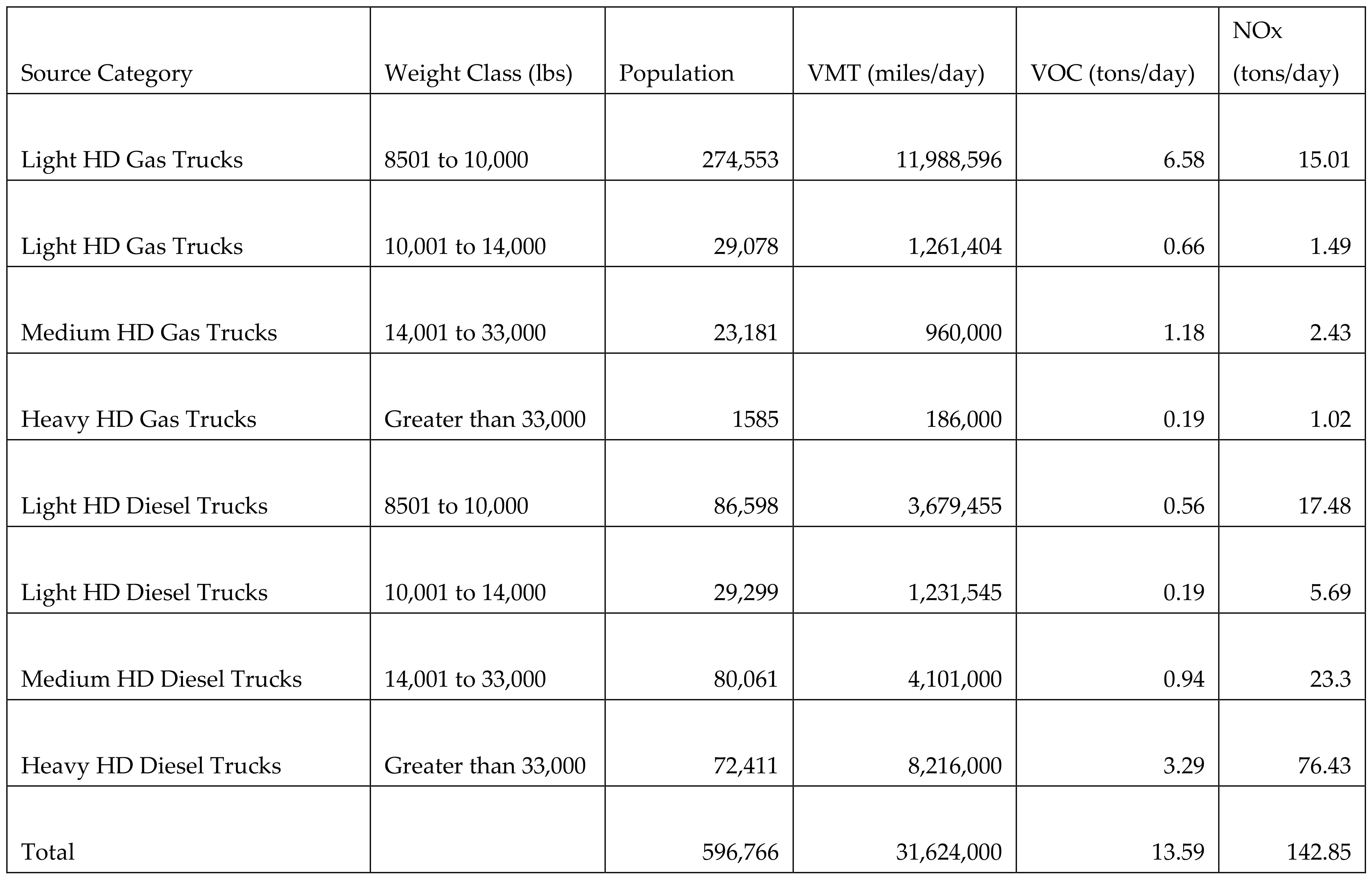
| Source Category | Population | VMT (Miles/Day) | VOC (Tons/Day) | VOC (% of Total) | NOx (Tons/Day) | NOx (% of Total) |
|---|---|---|---|---|---|---|
| Light HD Gas Trucks-1 (8501–10,000 lb.) | 274,553 | 11,988,596 | 6.58 | 48% | 15.01 | 11% |
| Light HD Gas Trucks-2 (10,001–14,000 lb.) | 29,078 | 1,261,404 | 0.66 | 5% | 1.49 | 1% |
| Medium HD Gas Trucks (14,001–33,000 lb.) | 23,181 | 960,000 | 1.18 | 9% | 2.43 | 2% |
| Heavy HD Gas Trucks (>33,000 lb.) | 1585 | 186,000 | 0.19 | 1% | 1.02 | <1% |
| Light HD Diesel Trucks-1 (8501–10,000 lb.) | 86,598 | 3,679,455 | 0.56 | 4% | 17.48 | 12% |
| Light HD Diesel Trucks-2 (10,001–14,000 lb.) | 29,299 | 1,231,545 | 0.19 | 1% | 5.69 | 4% |
| Medium HD Diesel Trucks (14,001–33,000 lb.) | 80,061 | 4,101,000 | 0.94 | 7% | 23.30 | 16% |
| Heavy HD Diesel Trucks (>33,001 lb.) | 72,411 | 8,216,000 | 3.29 | 24% | 76.43 | 54% |
| Total | 596,766 | 31,624,000 | 13.59 | 142.85 |
| Retailer | Market Share (2017) |
|---|---|
| Company A | 21% |
| Company B | 19% |
| Company C | 13% |
| Company D | 11% |
| Company E | 9% |
| Company F | 6% |
| Company G | 6% |
| Company H | 3% |
| Variable | Definition | Value | Source |
|---|---|---|---|
| di | Distance from shipment i’s entry point to central LA | 65, 75, or 225 miles | Google Maps |
| mi | 1 for internal LA shipment, 0 otherwise | FAF | |
| fi | 1 for mixed freight, 0 otherwise | FAF | |
| S | Food share of mixed freight | 35.6% | CFS |
| Ti | Ton miles for shipment i | FAF | |
| Ki | Kilotons in shipment i | FAF | |
| G | Industry share of food shipments | Grocery: 67% Food Service: 33% | Saksena et al., 2018 |
| A | Company’s grocery market share | Table 2 grocery market share (%) | LA Times, 2017 |
| O | Emissions: g/ton-mile CO2 | 87.75 | EPA SmartWay |
| N | Emissions: g/ton-mile NOx | 0.22 | EPA SmartWay |
| P | Emissions: g/ton-mile PM2.5 | 0.0035125 | EPA SmartWay |
| Retailer | CO2 Emissions (Tons Per Year) | NOx Emissions (Tons Per Year) | PM2.5 Emissions (Tons Per Year) | Local Air Pollution Cost (USD Millions Per Year) | Total Social Cost (USD Millions Per Year) |
|---|---|---|---|---|---|
| Company A | 84,769 | 212 | 3.4 | 7.5 | 11.3 |
| Company B | 76,951 | 193 | 3.1 | 6.8 | 10.2 |
| Company C | 54,730 | 137 | 2.2 | 4.8 | 7.3 |
| Company D | 46,500 | 117 | 1.9 | 4.1 | 6.2 |
| Other Grocery | 148,552 | 372 | 5.9 | 13.1 | 19.8 |
| Grocery Total | 411,501 | 1031 | 16.4 | 36.2 | 54.7 |
| Company I | 102,875 | 258 | 4.1 | 9.1 | 13.7 |
| Company J | 51,438 | 129 | 2.1 | 4.5 | 6.8 |
| Other Food Services | 51,438 | 129 | 2.1 | 4.5 | 6.8 |
| Food Services Total | 205,750 | 516 | 8.2 | 18.1 | 27.4 |
| Grand Total | 617,251 | 1547 | 24.6 | 54.3 | 82.1 |
| Variable | Definition |
|---|---|
| dx | Truck ton-miles associated with segment “x” |
| tx | Idling time associated with segment “x” |
| O | Driving emissions: g/mile CO2 |
| N | Driving emissions: g/mile NOx |
| P | Driving emissions: g/mile PM |
| Oh | Idling emissions: g/h CO2 |
| Nh | Idling emissions: g/h NOx |
| Ph | Idling emissions: g/h PM |
Publisher’s Note: MDPI stays neutral with regard to jurisdictional claims in published maps and institutional affiliations. |
© 2021 by the authors. Licensee MDPI, Basel, Switzerland. This article is an open access article distributed under the terms and conditions of the Creative Commons Attribution (CC BY) license (https://creativecommons.org/licenses/by/4.0/).
Share and Cite
Nowlan, A.; Fine, J.; O’Connor, T.; Burget, S. Pollution Accounting for Corporate Actions: Quantifying the Air Emissions and Impacts of Transportation System Choices Case Study: Food Freight and the Grocery Industry in Los Angeles. Sustainability 2021, 13, 10194. https://doi.org/10.3390/su131810194
Nowlan A, Fine J, O’Connor T, Burget S. Pollution Accounting for Corporate Actions: Quantifying the Air Emissions and Impacts of Transportation System Choices Case Study: Food Freight and the Grocery Industry in Los Angeles. Sustainability. 2021; 13(18):10194. https://doi.org/10.3390/su131810194
Chicago/Turabian StyleNowlan, Aileen, James Fine, Timothy O’Connor, and Spencer Burget. 2021. "Pollution Accounting for Corporate Actions: Quantifying the Air Emissions and Impacts of Transportation System Choices Case Study: Food Freight and the Grocery Industry in Los Angeles" Sustainability 13, no. 18: 10194. https://doi.org/10.3390/su131810194