Dynamic Inventory Routing and Pricing Problem with a Mixed Fleet of Electric and Conventional Urban Freight Vehicles

Abstract

Urban freight transport is essential for supporting our society regarding providing the daily needs of consumers and local businesses. In addition, it allows for the movement of goods, is distributed within urban environments, provides thousands of jobs, and supports economic growth. However, a number of issues are associated with urban freight transport, including environmental impacts, road congestion, and land use of freight facilities that conflicts with residential land use. Electric freight vehicles create zero emissions and provide a sustainable delivery system in comparison with conventional freight vehicles. In this study, a novel dynamic inventory routing and pricing problem under a mixed fleet of electric and conventional vehicles was formulated to minimize the total travel and charging costs. The proposed model is capable of deciding on replenishment times and amounts and vehicle routes. We aimed to determine the maximum social welfare (SW) capable of providing an optimal trade-off between the supplier cost and customer delay that uses a mixed fleet of vehicles. Our computational study was conducted on real data generated from a delivery dataset in Tehran. Under the proposed policy with a fleet of only electric vehicles, the SW increased by 3% while the average customer delay reduced by 15% compared with a fleet of conventional vehicles. The results show that the number of served customers and customer delay would be affected by transitioning conventional urban freight vehicles to electric vehicles. Therefore, the proposed delivery system has a significant impact on energy savings and emissions.

1. Introduction

The demand for the transport of goods within cities is rising while significant progress is being made in increasing the number of freight vehicles in daily city logistics operations. Many companies are striving to improve their supply chains by making them more transparent although conventional urban freight transport is a major contributor to greenhouse gases (GHGs) and is associated with substantially increased health risks. Hence, delivery companies in urban logistics must switch to zero-emission-capable road freight in urban areas using electric or hybrid trucks. Electric freight vehicles (EFVs) offer a potential solution for these issues. More precisely, they allow for the movement of goods and are distributed within an urban environment that reduces air and noise pollutions compared with conventional vehicles. However, the actual application of EFVs in urban logistics operations remains restricted.

EFVs become more competitive for logistic companies in order to save operational costs, leading to significantly increasing environmental benefits. However, the implementation of EFVs in urban logistic operations has several operational challenges, including charging, load capacity, and the limited range of energy. Therefore, vehicle routes should be precisely planned as a result of the limited range of vehicles. Our contributions include the following features:

(1)

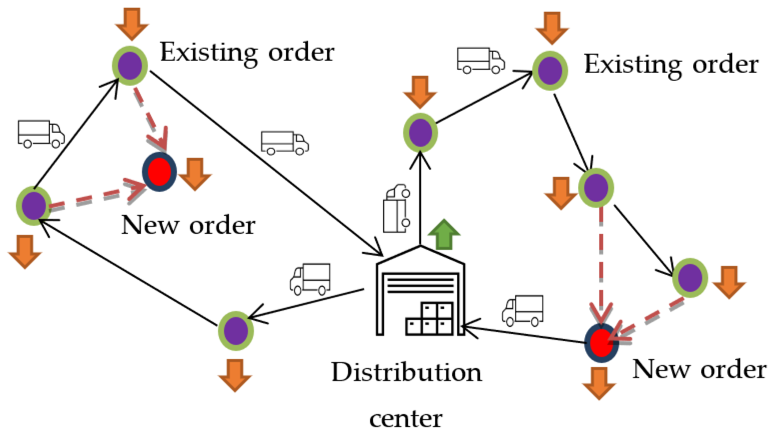
We propose a non-myopic dynamic inventory routing and pricing problem under a mixed fleet of electric and conventional vehicles.

(2)

We introduce a heterogeneous fleet of vehicles and use a realistic energy consumption that considers vehicle speed, cargo load and gradients, vehicle miles traveled (VMT), vehicle emissions, and charging costs.

(3)

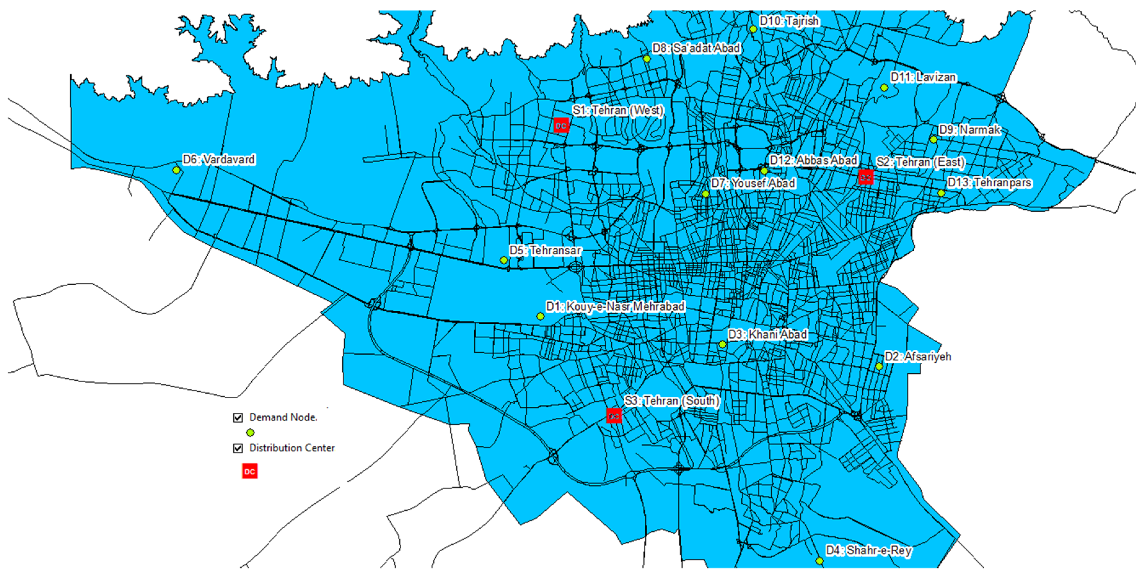
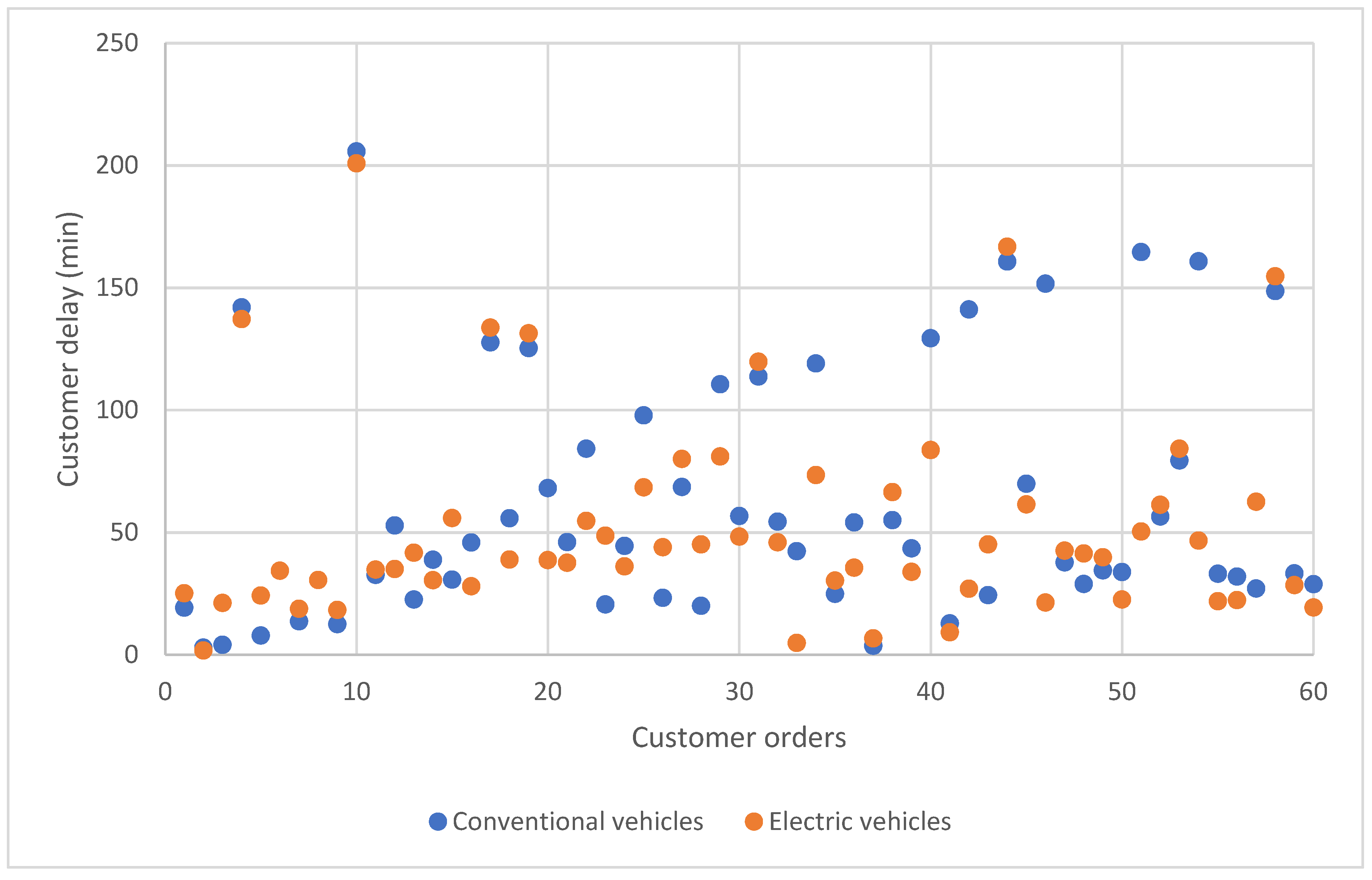
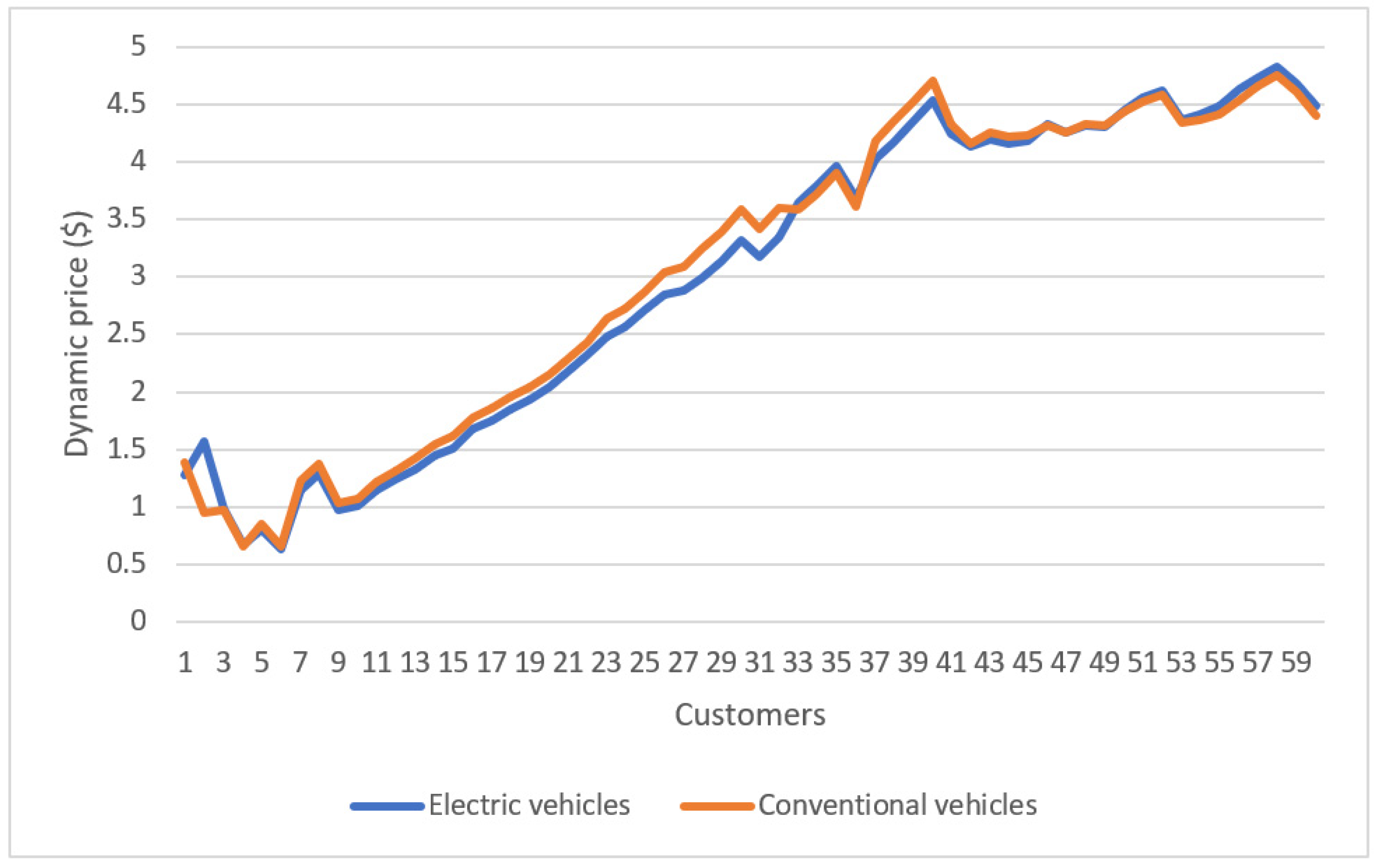
An empirical study is conducted on real data generated from a delivery dataset in Tehran that investigates both fleet sizing (conventional and electric vehicles) and allocation aiming at maximizing social welfare. The results show that the number of served customers and customer delay would be affected by transitioning conventional vehicles to electric vehicles.

Figure 1 presents an overview of the design of the inventory and delivery problem. The supply-chain optimization problems (e.g., the inventory routing problem) aiming at optimal joint decisions of inventory management, vehicle routing, and dispatching of urban freight vehicles have recently received considerable attention. In general, there is a set of pick-up nodes (suppliers) where a set of delivery nodes (customers) should be served by a mixed fleet of electric and conventional vehicles. The products are transported using a fleet of vehicles and customers gradually consuming the products. Pallets and boxes can be used to deliver the products from supply points to demand points. The items can be delivered by each vehicle that has a limited capacity. The type of truck route that must be taken depends on the origins and destinations of deliveries. Due to the activities of private logistics operators, three main classifications for road trucks based on weight are heavy, medium, and light trucks. Heavy-, medium-, and light-duty trucks are vehicles with a gross vehicle weight rating (GVWR) over 26,001 lbs, between 10,001 and 26,000 lbs, and under 10,000 lbs, respectively. This study focuses on a set of trucks to transport goods to a set of geographically scattered retailers.

In addition, the present study investigates a mixed fleet of conventional and EFV freight vehicles that must deliver orders to a set of geographically scattered customers over a long-term horizon look-ahead. The supplier takes on the responsibility of product deliveries and inventory management to customers. Further, a dynamic inventory routing problem is developed between supply and retailer nodes while considering an elastic demand (i.e., a demand that depends on inventory, routing, and pricing). A non-myopic approximation model for the specific case of a closed-loop supply chain problem is studied that considers future states. The policy aims to determine the optimal prices and the customers’ arrival rate in order to maximize social welfare (SW), which is computed as the difference between the revenue and the supplier and customer costs. The advantage of this method is its “self-regulating” nature since it encompasses different relationships between the effective arrival rate, replenishment times and amounts, vehicle route, dynamic price, and control service capacity that needs automation. These automated systems can be used in fully automated freight vehicles for a delivery system [1]. The remaining sections of this study are organized as follows:

Section 2 presents a relevant literature review on the topic to reveal the contribution of the research. A novel design of dynamic routing and the delivery of items under a mixed fleet of trucks is presented in Section 3, followed by an analysis of numerical examples and simulations of a real case in Section 4. Finally, Section 5 provides the concluding remarks.

2. Literature Review

Electric freight vehicles are much more energy efficient compared with conventional freight vehicles, and, therefore, are expected to bring considerable energy savings to urban freight. For example, [2,3] studied several approaches to solve the EVR under partial recharge and multiple recharging technologies for using EFVs. Similarly, [4] proposed a vehicle routing problem related to the use of EFVs under a limited capacity of the battery. Likewise, [5,6] investigated a delivery problem for urban trucks that considers power consumption for managing a limited battery capacity. The authors of [7] proposed a static VRP model under a mixed fleet of electric and conventional trucks while considering linear energy consumption. The authors of [8] proposed a mixed-integer linear programming method for a delivery routing problem with a mixed fleet of electric and conventional vehicles. The authors of [9] also introduced an electric vehicle routing problem (EVRP) model that evaluates slow and fast recharging stations by a nonlinear charging approach. Furthermore, [10] studied an EVRP model with recharging stations under a mixed fleet of vehicles. Moreover, [11] extended the model that focuses on a combined fleet of vehicles, such as conventional, plug-in hybrid, and electric vehicles.

Many existing studies have also considered the design of recharging infrastructures in the EVRP. For example, [12] studied a routing-location problem under stochastic demands aiming at minimizing the total cost including the construction cost of the recharging station and the expected traveling cost of the route. In their study, the authors of [13] investigated a two-stage mixed-integer linear program for an EVRP with a stochastic waiting time at recharging stations. Additionally, [14] proposed a Markov decision process (MDP) for an EVRP with a stochastic waiting time at public recharging stations. In another study, [15], the authors introduced a robust optimization location-routing framework that considers the problem of simultaneously routing vehicles and locating charging stations.

To the best of our knowledge, most studies in this area are related to the EVRP in the context of stochastic decision-making problems. For instance, [16] presented a stochastic EVRP without en-route recharging under a stochastic power consumption function. Strategies that consider future states are defined as non-myopic policies. However, a limited body of research has addressed the dynamic routing of electric vehicles under a non-myopic policy. For example, [17] evaluated online EVs with battery swaps as an MDP using an approximated dynamic programming method with linear temporal differencing. The authors of [18] introduced a new social-based optimization model for the distribution of batteries, where the approach comprises decisions related to loaded and unloaded batteries, routing, and scheduling of vehicles between the battery charging and battery swapping stations. A summary of recent contributions to routing and delivery systems is described in

Table 1. Summary of routing and delivery studies.

Studies	Model Feature(s)
[19]	Incorporated energy consumption in a myopic electric routing problem while not considering vehicle loads.
[20]	Introduced mixed-integer linear programming for the probabilistic inventory routing problem with a homogenous vehicle that considers emissions and energy consumption.
[16]	Minimized the total costs of a myopic electric routing problem.
[21]	Introduced mixed-integer linear programming for a production inventory and delivery problem with a heterogeneous vehicle while not considering energy consumption and environmental concerns.
[18]	Maximized social welfare for the non-myopic distribution of the electric battery problem with homogeneous vehicles while not considering energy consumption, vehicle loads, and environmental concerns.
Current paper	Integrated the non-myopic dynamic optimization of routing, transportation, and inventory with a heterogeneous fleet of vehicles that considers energy consumption and environmental impacts.

.

This study proposes a new routing and scheduling model that considers replenishment times and amounts under a mixed fleet for urban freight transportation problems, stemming from the work of [18]. Currently, there are no dynamic models with a look-ahead policy that incorporate heterogeneous electric freight vehicles and use energy consumption for the problem analysis. In addition, no model has so far investigated both fleet sizing (conventional and electric vehicles) and allocation aiming at maximizing SW or considered a dynamic dispatch system by taking into account the future state that minimizes the total travel and charging costs. Using the real-time urban freight dataset, we show that both customers and system providers are satisfied by the proposed methodology.

3. The Mathematical Model

The proposed algorithm starts by determining the load size, the effective arrival rates, the reward upon completion of service, and the degree of look-ahead for each new customer, followed by updating the locations and service states of the tours determined for the previous analyzed customer. Then, an optimization formulation Problem 1 is applied for each truck to obtain a potential tour, and the optimal arrival rate of the current customer is derived, along with the system revenue. Finally, the truck maximizing SW is chosen, and the potential tour is updated with the selected one while keeping all the others the same as before. In summary, there are three simultaneous decisions to make, including how much to deliver when serving a customer under a mixed fleet of conventional and electric freight trucks, how to route the vehicle among the customers to be served, and when to serve a customer and the amounts.

Table 2. Input parameters and outputs of the proposed model.

Symbol	Description
Indices and sets
$\mathit{i},\mathit{j}$	vertex	$\mathsf{\varpi }$	the fuel-to-air mass ratio
$p$	supply nodes	$\mathsf{\chi }$	the heating value of a typical diesel fuel
$t$	time periods	$\mathsf{\varsigma }$	the conversion factor
$N$	the set of all points in the network	$\varrho$	$\varrho =0.5C_d\rho A$
$S$	the set of the supply nodes, $S\subset N$	$C_d$	expected air drag coefficient
$D$	the set of the demand nodes, $D\subset N$	$\rho$	expected air density
$\tau$	the current location of the trucks, $\tau \in N$	$A$	frontal area
$e$	the dummy end node that all trucks will go to at the end of their tour, $e\in N$	$\gamma$	$\gamma =(1/1000\mho \mathsf{\Psi })$
$T$	the set of needed steps to finish the delivery	$\mho$	efficiency parameter for diesel engines
$O_i$	the number of orders of customer nodes $i\in D$	$\pi$	$\pi =g\sin \left(\alpha \right)+g{C}_r\cos \left(\alpha \right)$
$S_i$	maximum supply nodes $i\in S$	$C_r$	rolling friction coefficient
$K$	the capacity of the truck	$\alpha$	road angle (rad)
$l_0$	an initial load of the truck	$g$	gravitational constant
$d_{ij}$	the distance between points $i$ and $j\in N$	$\vartheta$	curb-weight (kg)
${\Delta }_{ij}$	truck speed (km/h)	$w$	the weight of a full load of items
$\eta$	$\eta =ℒ\varkappa \mathscr{H}$	${\mathsf{\Gamma }}_1$	the energy consumption cost of a conventional vehicle
$ℒ$	the engine displacement	${\mathsf{\Gamma }}_2$	the energy consumption cost of an electric vehicle
$\varkappa$	the engine speed	$\phi$	auxiliary power demand ($W$)
$\mathscr{H}$	the engine friction factor	$\mathsf{\Psi }$	vehicle drivetrain efficiency
$\delta$	$\delta =\mathsf{\varpi }/(\mathsf{\varsigma }\mathsf{\chi })$	$V_f$	type of fuel $f=\left\{1,2\right\}$, where 1 refers to conventional freight vehicles and 2 refers to electric freight vehicles, $v_f=\left\{1,\dots ,\left|V_f\right|\right\}$
Decision variables
$x_{ijt}$	if the truck goes from $i\in N$ to $j\in N$ at step $t$ 1; otherwise 0
$y_{ijt}$	the number of loaded items on the truck going from $i\in N$ to $j\in N$ at step $t$
$l_{it}$	the number of loaded items in $i\in S$ by the truck at time period $t$
$u_{it}$	the number of unloaded items in $i\in D$ by the truck at time period $t$

presents the input and outputs of Problem 1.

3.1. Energy Consumption

The total amount of fuel for the conventional freight vehicle $C$ is calculated by the engine module, which is linear in the travel cost and investigates vehicle speed and cargo load, and gradients [22,23,24,25].

Table 3. Model parameter values.

Parameter	Description	Value	Parameter	Description	Value
$\eta$	$\eta =ℒ\varkappa \mathscr{H}$	33	$w$	the weight of a full load of items	20 kg
$ℒ$	engine displacement	5$\left(\mathrm{l}\right)$	${\mathsf{\Gamma }}_1$	the energy consumption cost of a conventional vehicle	1.4
$\varkappa$	engine speed	33$\left(\mathrm{rev}/\mathrm{s}\right)$	${\mathsf{\Gamma }}_2$	the energy consumption cost of an electric vehicle	0.2
$\mathscr{H}$	engine friction factor	0.2$\left(\mathrm{kJ}/\mathrm{rev}/\mathrm{liter}\right)$	$\phi$	auxiliary power demand ($\mathrm{W}$)	1575
$\delta$	$\delta =\mathsf{\varpi }/(\mathsf{\varsigma }\mathsf{\chi })$	0.00003	$\mathsf{\Psi }$	vehicle drivetrain efficiency	0.4
$\mathsf{\varpi }$	fuel-to-air mass ratio (air–fuel equivalence ratio (AFR), $\mathsf{\varpi }$, is the ratio of actual AFR to stoichiometry for a given mixture $\mathsf{\varpi }=1.0$ is at stoichiometry [29,30])	1	$O$	the number of orders	3951 items
$\mathsf{\chi }$	heating value of a typical diesel fuel	44 ($\mathrm{kJ}/\mathrm{g})$	$\sigma$	the rate of waiting cost	$1
$\mathsf{\varsigma }$	conversion factor	737 ($\mathrm{g}/\mathrm{L})$	$N_d$	the number of supply points	30
$\varrho$	$\varrho =0.5C_d\rho A$ (conventional and electrical trucks)	2.889840, 1.6486537	$N_s$	the number of demand points	5
$C_d$	expected air drag coefficient (conventional and electrical trucks)	0.6, 0.7	$C$	the capacity of items at supply nodes	2500, 2000, 3000
$\rho$	expected air density	1.2041 $\mathrm{kg}/{\mathrm{m}}^3$	$V$	the number of vehicles	10
$A$	frontal area (conventional and electrical trucks)	8, 3.912 ${\mathrm{m}}^2$	$R$	a reward for service	15
$\gamma$	$\gamma =(1/1000\mho \mathsf{\Psi })$	0.005	$\theta$	a weight	0.5
$\mho$	efficiency parameter for diesel engines	0.5	$\hat{\mu }$	the service rate	6
$\pi$	$\pi =g\sin \left(\alpha \right)+g{C}_r\cos \left(\alpha \right)$	0.0981	$\Lambda$	the aggregate arrival rate	4
$C_r$	rolling friction coefficient	0.01	$K$	vehicle capacity	100
$\alpha$	road angle (rad)	0	$\mathsf{\Omega }$	the value of time	0.33
$g$	gravitational constant	9.81($\mathrm{m}/{\mathrm{s}}^2$)	$\beta$	degree of look-ahead	0.2
$\vartheta$	curb-weight (kg)	6350 kg	$\left|T\right|$	the set of needed steps to finish the plan	25
${\Delta }_{ij}$	vehicle speed ($\mathrm{km}/\mathrm{h}$)	40

presents the notations and parameters.

$$C_{ij}={\delta }_k\left({\eta }_k\left(\frac{d_{ij}}{{\Delta }_{ij}}\right)+\left({\gamma }_k{\varrho }_{k1}{d}_{ij}{\Delta }_{ij}{}^2\right)+{\gamma }_k{\pi }_{k1}\left({\vartheta }_{k1}+w_l\right)d_{ij}\right)$$

(1)

Likewise, the total amount of the energy consumption of the road segment for electric freight vehicle $E$ is computed by [16,23,26]

$$e_{ij}=\frac{\left({\varrho }_{k2}{d}_{ij}{\Delta }_{ij}{}^2\right)+{\pi }_{k2}\left({\vartheta }_{k2}+w_l\right)d_{ij}}{3.6\times {10}^6}$$

(2)

$$\mathrm{E}=\{\begin{array}{c}{\Psi }_{k2}.e_{ij}+\frac{{\phi }_k{t}_{ij}}{3.6\times {10}^6},if{e}_{ij}\ge 0\\ \frac{{\phi }_k{t}_{ij}}{3.6\times {10}^6}if{e}_{ij}<0\end{array}$$

(3)

3.2. Incorporating Uncertainty

In this section, a value function in terms of SW under the infinite-horizon look-ahead is determined using the demand function that considers a one-to-one connection between non-myopic pricing and effective customers joining the system, the supplier costs (in terms of the length of tours under a mixed fleet of urban trucks), and the expected customer delay. In this study, an approximation method is proposed to investigate future states by examining the trade-off between “exploitation” and “exploration” policies [27,28]. This study applies an approximation approach according to [18]:

$$\left\{{\hat{\xi }}_n^{*},{\hat{l}}_{v*},{\hat{u}}_{v*},{\hat{y}}_{v*},{\hat{p}}_n^{*}\right\}=\arg \underset{\mathsf{\chi }}{\max }\left[SW\left({\hat{\lambda }}_n;{\hat{\xi }}_n,{\hat{l}}_v,{\hat{u}}_v,{\hat{y}}_v,{\hat{p}}_n\right)-SW\left({\hat{\lambda }}_n;{\hat{\xi }}_{n-1},{\hat{l}}_v,{\hat{u}}_v,{\hat{y}}_v,{\hat{p}}_{n-1}\right)\right],$$

(4)

where $SW\left({\hat{\lambda }}_n;{\hat{\xi }}_n^{*},{\hat{l}}_{v*},{\hat{u}}_{v*},{\hat{y}}_{v*},{\hat{p}}_n^{*}\right)$ is the SW function and $v_f$ represents the set of vehicles by sizes $v$ and the type of fuels $f=\left\{1,2\right\}$, where 1 refers to conventional freight vehicles and 2 refers to electric freight vehicles, $v_f=\left\{1,\dots ,\left|V_f\right|\right\}$. Let $\mathsf{\chi }$ indicate the set of decision variables that contains an optimal decision on replenishment times and amounts where ${\hat{l}}_{v*}$ denotes the optimal number of loaded items at supply nodes and ${\hat{u}}_{v*}$ is the optimal number of unloaded items delivered to customer nodes. In addition, ${\hat{y}}_v$ is the number of loaded items on the vehicle. Further, ${\hat{\xi }}_n^{*}$ is a new tour upon the arrival of a customer and places a new request for new items, and, finally, ${\hat{p}}_n^{*}$ represents the optimal price [18].

$$\begin{array}{cc}\hfill SW\left({\hat{\lambda }}_n;{\hat{\xi }}_n,{\hat{l}}_v,{\hat{u}}_v,{\hat{y}}_v,{\hat{p}}_n\right)& =\Lambda R\frac{1-{\mathsf{\rho }}^{\left(R-{\hat{p}}_n\right)\hat{\mu }}}{1-{\mathsf{\rho }}^{\left(R-{\hat{p}}_n\right)\hat{\mu }+1}}-\frac{\theta }{T\left({\hat{\xi }}_n,{\hat{l}}_v,{\hat{u}}_v,{\hat{y}}_v\right)}\left(T\left({\hat{\xi }}_n,{\hat{l}}_v,{\hat{u}}_v,{\hat{y}}_v\right)-\frac{\psi {\hat{\lambda }}_n}{{\left(\hat{\mu }-{\hat{\lambda }}_n\right)}^2}\right)\hfill \\ & -\frac{\left(1-\theta \right)}{T\left({\hat{\xi }}_n,{\hat{l}}_v,{\hat{u}}_v,{\hat{y}}_v\right)}\left({\displaystyle \sum }_{i=1}^n{S}_i\left({\hat{\xi }}_n,{\hat{l}}_v,{\hat{u}}_v,{\hat{y}}_v\right)+\frac{\hat{\mu }{\hat{\lambda }}_n}{2\left(\hat{\mu }-{\hat{\lambda }}_n\right)}T{\left({\hat{\xi }}_n,{\hat{l}}_v,{\hat{u}}_v,{\hat{y}}_v\right)}^2+\frac{\psi {\hat{\lambda }}_n}{{\left(\hat{\mu }-{\hat{\lambda }}_n\right)}^2}\right)\hfill \end{array}$$

(5)

$$k\left({\hat{p}}_n\right)\le \left[\left(R-{\hat{p}}_n\right)\hat{\mu }/\sigma \right]$$

(6)

$$0<{\lambda }_n\le \Lambda$$

(7)

where $T\left({\hat{\xi }}_n,{\hat{l}}_v,{\hat{u}}_v,{\hat{y}}_v\right)$ is the length of a tour by vehicle $v$, which is determined by solving an optimization module (Section 3.2.1). ${\sum }_{i=1}^n{S}_i\left({\hat{\xi }}_n,{\hat{l}}_v,{\hat{u}}_v,{\hat{y}}_v\right)$ denotes the total sojourn time, which is obtained from the simulation module regarding the potential tours ${\hat{\xi }}_n$. A weight differentiating the objectives is selected by $\theta$, $0\le \theta \le 1,$ and $\beta$ is the policy parameters that differentiate among non-myopic policies and myopic policies.

3.2.1. Mathematical Formulation

An optimization formulation is run to obtain potential tours. It aims to minimize the traveled distance by the mixed fleet of vehicles to visit customers in a distribution and transportation network. The objective function (8) of this study is to minimize the total charging costs, composed of two terms. The first and the second terms correspond to the sum of the total charging costs under the conventional freight vehicle and the electric freight vehicle, respectively.

Problem 1: Integrated optimization of routing and inventory with a mixed fleet of electric and conventional vehicles

$$\begin{array}{c}\mathrm{Z}=\min {\displaystyle \sum }_{i\in N}{\displaystyle \sum }_{j\in N}{\displaystyle \sum }_{t\in T}\delta \left(\left(\frac{\eta }{{\Delta }_{ij}}+\gamma \varrho {\Delta }_{ij}{}^2+\gamma \pi \vartheta \right)d_{ij}{x}_{ijt}+\gamma \pi w{d}_{ij}{y}_{ijt}\right){\mathsf{\Gamma }}_1\\ +{\displaystyle \sum }_{i\in N}{\displaystyle \sum }_{j\in N}{\displaystyle \sum }_{t\in T}\left[\mathsf{\Psi }Va{r}_{ijt}+\left(\frac{\phi \left(\frac{d_{ij}}{{\Delta }_{ij}}\right)}{3.6\times {10}^6}\right)x_{ijt}\right]{\mathsf{\Gamma }}_2\end{array}$$

(8)

Subject to:

$$Va{r}_{ijt}\ge \frac{\left(\varrho {\Delta }_{ij}{}^2+\pi \vartheta \right)d_{ij}{x}_{ijt}+\pi w{d}_{ij}{y}_{ijt}}{3.6\times {10}^6}\forall i,j\in N,t\in T$$

(9)

$${\displaystyle \sum }_{j\ne \tau }{x}_{\tau j1}=1$$

(10)

$$x_{\tau jt}=0\forall j\in N,t\ge 2$$

(11)

$${\displaystyle \sum }_{\begin{array}{c}j\in N\\ j\ne i\end{array}}{x}_{ijt}={\displaystyle \sum }_{\begin{array}{c}j\in N\\ j\notin \left\{i,e\right\}\end{array}}{x}_{jit-1}\forall i\in N\backslash \left\{\tau ,e\right\},t\ge 2$$

(12)

$${\displaystyle \sum }_{i\in N}{\displaystyle \sum }_{j\in N}{x}_{ijt}=1\forall t\in T$$

(13)

$$x_{ejt}=0\forall j\in N,t\in T$$

(14)

$${\displaystyle \sum }_{i\in N}{\displaystyle \sum }_{t\in T}{x}_{iet}=1$$

(15)

$$y_{ijt}\le K{x}_{ijt}\forall i\in N,j\in N,t\in T$$

(16)

$${\displaystyle \sum }_{j\in N}{y}_{ijt}={\displaystyle \sum }_{j\in N}{y}_{jit-1}-u_{it}\forall i\in D,t\ge 2$$

(17)

$${\displaystyle \sum }_{j\in N}{y}_{ijt}={\displaystyle \sum }_{j\in N}{y}_{jit-1}+l_{it}i\in S,\forall t\ge 2$$

(18)

$${\displaystyle \sum }_{j\in N}{y}_{\tau j1}=l_0$$

(19)

$$l_0+{\displaystyle \sum }_{i\in S}{\displaystyle \sum }_{t\in T}{l}_{it}={\displaystyle \sum }_{i\in D}{\displaystyle \sum }_{t\in T}{u}_{it}$$

(20)

$${\displaystyle \sum }_{t\in T}{l}_{it}\le {\mathrm{S}}_i\forall i\in S$$

(21)

$${\displaystyle \sum }_t{u}_{it}=O_{i}i\in D$$

(22)

$$u_{i1}=0\forall i\in N$$

(23)

$$x_{ijt}\in \left\{0,1\right\},y_{ijt}\ge 0,l_{it}\ge 0,u_{it}\ge 0Va{r}_{ijt}\ge 0,\forall i,j\in N,t\in T$$

(24)

The fuel rate of electric vehicles for a path is presented by constraint (9). The flow equivalence in the nodes is guaranteed by constraints (10)–(15). Constraints (17) and (20) cover the case with the loading and unloading of items in the demand/supply nodes. The dummy node is defined to remove the necessity of returning a truck to the initial point. Constraint (18) guarantees that the truck will not pick more items than what is needed for demand points in its scheduled route. Constraints (16)–(21) guarantee that the load of the truck and all picked items from a supply node will not violate the capacity of the truck limitation at the supply node, respectively. The provision of the needed demand for each customer node is stated in constraints (22) and (23). Finally, the type of variable is defined by constraint (24).

The following algorithm, called Algorithm 1, is applied in the online operational routing and delivery problem (and for simulated runs). The status of each truck location regarding the supply and demand nodes is updated upon the arrival of a new request. The remaining tour ($\xi$) shows the status of a mixed fleet of trucks $v\in \left\{V_1,V_2\right\}$, where $V_1$ denotes a set of conventional trucks and $V_2$ refers to a set of electrical trucks. The initially loaded items in the truck and the currently loaded items are determined by $l_0$ and $l$, respectively. The set of all nodes in network $N$ is determined by supply points in the route of the truck ($dem\left(v.\xi \right)$), the new demand points ($n$), and the dummy end node ($e$). The distance between points $d_{ij}$ is determined where the distance between points and the dummy nodes is zero. Then, the inventory and routing with the mixed fleet model are solved and are shown by constraints (8), along with constraint (24) for the given parameters of the truck $v$, the nodes $N$, the capacity of supply nodes $C$, and the demand of customers $O$. The SW function is maximized to find the best decisions, such as the best truck ($v^{*}$) and the optimal delivery items and routes between supply and demand nodes. Eventually, the outputs include the effective optimal arrival time, fare prices, and the sequence of customers visited by each truck and the tour length.

Algorithm 1. Integrated optimization of vehicle routing, transportation, and inventory with the mixed fleet of vehicles

Step 0. Initialization: Input parameters. For $i\in n$

For $v\in \left\{V_1,V_2\right\}$:

Step 1.

Update $v.\left(\xi ,l,l_0\right)$

$N\leftarrow N_s\cup dem\left(v.\xi \right)\cup \left\{n\right\}\cup \left\{v.l\right\}\cup \left\{e\right\}$

$\left[d_{ij}\right]\leftarrow distance\left(N\right)$

${\hat{\xi }}_v,{\hat{l}}_v,{\hat{u}}_v\leftarrow IRMF\left(v,N,\left[d_{ij}\right],C,O\right)$

Step 2.

Compute

$SW\left({\hat{\lambda }}_n;{\hat{\xi }}_n,{\hat{l}}_v,{\hat{u}}_v,{\hat{p}}_n\right)\leftarrow T\left({\hat{\xi }}_n,{\hat{l}}_v,{\hat{u}}_v\right)$

${\hat{\lambda }}_n^{*}\leftarrow \left[\partial D\left({\hat{p}}_n\right)/\partial {\lambda }_n=0\right]$

Step 3.

Calculate

$v^{*}\leftarrow \underset{v\in V}{\mathrm{argmax}}\left\{SW\left({\hat{\lambda }}_n;{\hat{\xi }}_n,{\hat{l}}_v,{\hat{u}}_v,{\hat{p}}_n\right)-SW\left({\hat{\lambda }}_n;{\hat{\xi }}_{n-1},{\hat{l}}_v,{\hat{u}}_v,{\hat{p}}_{n-1}\right)\right\}$

$v^{*}.\left(\lambda ;\xi ,l,u,p\right)\leftarrow \left({\hat{\lambda }}_n^{*};{\hat{\xi }}_n^{*},{\hat{l}}_{v*},{\hat{u}}_{v*},{\hat{p}}_n^{*}\right)$

end

end

4. Results

This section describes our tests of the proposed dynamic model. Section 4.1 explains the generation of our test data. In Section 4.2, the efficiency of our proposed approach is demonstrated in a real-life case study, and scenarios are created in a distribution company in Tehran. The main point of the proposed model is an online delivery of items from supply points to demand points under a mixed fleet of trucks. The branch and bound (B&B) algorithm was implemented using Matlab, running on a desktop with an Intel^® Core™ i5-8550U processor with 16GB of RAM and a 64-bit platform using a Windows 10 operating system.

4.1. Data Collection

For testing, our computational study was run on real data generated from the daily activity of a distribution company in Tehran. The selected area includes three suppliers ($S_1,S_2,S_3$) that serve 13 demand nodes ($D_1\dots ,D_{13}$). The distribution company is presently one of the largest delivery companies in Iran. It blends, packs, sells, and deliveries teas as well as a wide variety of other types of food products, including rice, spices, pistachios, saffron, and so forth. The effects of other types of urban freight vehicles, such as refrigerated trucks, on the charging cost and energy consumption will be modeled in a future study. Figure 2 shows the distribution of items between the supply and demand networks.

The travel cost between road intersections was determined by the Euclidean distance method. The customer arrival rate $\hat{\lambda }$ of items at each demand node appears as the Poisson process and was computed by the historical dataset of a distribution company. The service rate $\hat{\mu }$ of items at each supply node was assumed to follow an exponential distribution and was calculated by the service times from the historical dataset. Table 3 presents the applied input parameters in our simulations.

4.2. Experimental Results

In the following section, the routing and delivery system is examined under the fleet of only electric vehicles or the fleet of only conventional vehicles, followed by evaluating the impact of feet size and demand rates on the performance of the distribution model.

Table 4. The results of only electric vehicles.

Vehicles	Optimal Routes and Replenishment Times and Amounts
${\mathit{V}}_{\mathbf{1}}$	Route: S1–D3–S3–D3–S3–D3–S3–D3–S3–D1–S3–D1–S3–D6–S3–D6
	Time: 6.96–30.53–33.39–36.26–39.13–42.00–44.87–47.73–50.60–75.26–85.73–96.20–106.68–144.11–177.87–211.63
	Load/unload: 80, 42, −42, 57, −57, 19, −19, 73, −73, 80, −80
${\mathit{V}}_{\mathbf{2}}$	Route: S2–D7–S3–D7–S3–D7–S3–D7–S3–D7–S3–D7
	Time: 10.33–28.66–37.54–46.42–55.30–64.18–73.06–81.94–90.83–99.71–108.59–117.47
	Load/unload: 61, −61, 76, −76, 80, −80, 80, −80, 14, −14, 80, −80
${\mathit{V}}_{\mathbf{3}}$	Route: S3–D3–S3–D4–S3–D8–S1–D8–S1–D8–S1–D8–S1–D8–S1–D8
	Time: 1.70–4.77–7.64–26.83–46.01–64.53–66.71–68.89–71.07–73.25–75.43–77.62–79.80–81.98–84.16–86.34
	Load/unload: 66, −25, 25, −66, 55, −55, 46, −46, 80, −80, 80, −80, 80, −80, 80, −80
${\mathit{V}}_{\mathbf{4}}$	Route: S1–D13–S2–D11–S2–D13–S2–D13–S2–D11–S2–D13–S2–D13
	Time: 7.10–31.27–39.13–43.17–47.22–55.07–62.93–70.78–78.64–82.68–86.73–94.58–102.44–110.29
	Load/unload: 73, −73, 62, −62, 79, −79, 80, −80, 44, −44, 80, −80, 80, −80
${\mathit{V}}_{\mathbf{5}}$	Route: S3–D1–S3–D2–S3–D2
	Time: 36.14–46.62–57.09–70.75–84.41–98.07
	Load/unload: 75, −75, 24, −24, 64, −64
${\mathit{V}}_{\mathbf{6}}$	Route: S3–D11–S2–S2–D10–S1–D10–S1–D10–S1–D10–S1–D10–S1–D10–S1–D10
	Time: 4.96–26.15–30.19–35.30–48.96–57.06–65.16–73.26–81.37–89.47–97.57–105.67–113.77–121.87–129.97–138.07–146.17
	Load/unload: 54, −54, 21, 4, −25, 80, −80, 80, −80, 80, −80, 80, −80, 80, −80, 63, −63
${\mathit{V}}_{\mathbf{7}}$	Route: S1–D5–S3–D12–S3–D12–S3–D12–S3–D12–S3–D12
	Time: 8.24–26.97–41.08–52.73–64.39–76.04–87.69–99.35–111.00–122.66–134.31–145.97
	Load/unload: 55, −55, 77, −77, 80, −80, 80, −80, 80, −80, 36, −36
${\mathit{V}}_{\mathbf{8}}$	Route: S2–S3–D1–S3–D11–S2–D11–S3–D4
	Time: 12.52–37.06–47.54–58.01–79.19–83.24–87.28–108.46–127.65
	Load/unload: 35, 35, −70, 56, −56, 58, −58, 57, −57
${\mathit{V}}_{\mathbf{9}}$	Route: S3–D5–S3–D9–S2–D9–S1–D6–S1–D6
	Time: 10.81–55.73–69.41–90.61–94.79–98.96–121.10–154.85–188.61–222.37
	Load/unload: 61, −33, 27, −55, 80, −80, 80, −80, 80, −80
${\mathit{V}}_{\mathbf{10}}$	Route: S1–D9–S2–D9–S2–S2–D10–S1–D10–S1–D10–S1–D10
	Time: 10.17–32.31–36.48–40.66–44.84–47.85–61.51–69.61–77.71–85.81–93.91–102.01–110.11
	Load/unload: 44, −44, 80, −80, 66, 5, −71, 80, −80, 62, −62, 80, −80

provides the results of vehicle routes, loading/unloading of items, and times under the fleet of only electric vehicles. The VMTs for only electric vehicles are 172.7501, 84.86096, 70.232, 34.077, 73.058, 102.920, 102.119, 102.227, 177.344, and 75.408 km, respectively.

Then, the impact of the feet size on the performance of the delivery system was studied. Fleet sizes $V$ are considered in the range 9–15. Next, the VMT and the amount of emissions were determined for each fleet size.

Table 5. The results of only conventional vehicles.

Vehicles	Optimal Routes and Replenishment Times and Amounts
${\mathit{V}}_{\mathbf{1}}$	Route: S1–D3–S3–D3–S3–D3–S3–S3–D1–S3–D6–S1–D6
	Time: 6.96–30.53–33.39–36.26–39.13–42.00–44.87–90.55–101.02–111.49–148.93–182.69–216.45
	Load/unload: 57, −57, 80, −80, 43, −43, 57, 19, −76, 73, −73, 80, −80
${\mathit{V}}_{\mathbf{2}}$	Route: S2–D11–S2–S3–D7–S3–D7–S3–D7–S3–D7–S3–D7
	Time: 4.96–9.01–20.06–45.97–54.85–63.73–72.61–81.49–90.37–99.26–108.14–117.02–125.90
	Load/unload: 54, −54, 56, 24, −80, 80, −80, 80, −80, 80, −80, 10, −10
${\mathit{V}}_{\mathbf{3}}$	Route: S3–D4–S3–D3–S3–S1–D10–S1–D10–S1–D10–S1–D10–S1–S10–S1–D10–S1–D10–S1–D10–S1–D10–S1–D10
	Time: 1.70–20.89–41.84–44.71–48.77–70.33–78.43–86.54–94.64–102.74–110.84–118.94–127.04–135.14–143.24–151.34–159.44–167.54–175.64–183.74–191.84–199.95–208.05–216.15–224.25
	Load/unload: 66, −66, 53, −42, 5, 64, −80, 61, −61, 80, −80, 80, −80, 80, −80, 80, −80, 80, −80, 80, −80, 80, −80, 80, −80
${\mathit{V}}_{\mathbf{4}}$	Route: S1–D9–S2–D9–S2–D2–S3–D2
	Time: 10.17–32.31–36.48–40.66–44.84–65.34–78.99–92.65
	Load/unload: 44, −44, 80, −80, 24, −24, 64, −64
${\mathit{V}}_{\mathbf{5}}$	Route: S2–D13–S1–D8–S1–D8–S1–D8–S1–D9–S2–D9
	Time: 7.10–14.95–41.61–43.79–45.97–48.15–50.34–52.52–56.04–78.17–82.35–86.53
	Load/unload: 73, −73, 80, −80, 55, −55, 80, −80, 76, −76, 59, −59
${\mathit{V}}_{\mathbf{6}}$	Route: S3–D3–S3–D13–S2–D13–S2–D13–S2–D13–S2–D13
	Time: 3.04–5.91–16.30–36.02–43.87–51.73–59.58–67.44–75.29–83.15–91.00–98.86
	Load/unload: 25, −25, 75, −75, 4, −4, 80, −80, 80, −80, 80, −80
${\mathit{V}}_{\mathbf{7}}$	Route: S1–D7–S3–D10–S3–D12–S3–D12–S3–D12–S3–D12
	Time: 10.33–22.80–36.28–47.93–59.59–71.24–82.90–94.55–106.21–117.86–129.52–141.17
	Load/unload: 61, −61, 80, −80, 72, −72, 80, −80, 80, −80, 41, −41
${\mathit{V}}_{\mathbf{8}}$	Route: S2–D1–S3–D1–S1–D8–S1–D8–S1–D8
	Time: 11.85–44.43–54.91–65.38–86.64–88.82–91.00–93.19–95.37–97.55
	Load/unload: 75, −75, 70, −70, 80, −80, 80, −80, 46, −46
${\mathit{V}}_{\mathbf{9}}$	Route: S3–D5–S3–S2–D11–S2–D11–S2–D11
	Time: 8.24–21.92–52.03–76.62–80.66–84.71–88.75–92.80–96.84
	Load/unload: 55, −55, 38, 42, −80, 80, −80, 60, −60
${\mathit{V}}_{\mathbf{10}}$	Route: S1–D5–S3–D4–S3–D6–S1–D6
	Time: 10.81–59.33–73.01–92.19–111.38–148.81–182.57–216.33
	Load/unload: 61, −33, 29, −57, 80, −80, 80, −80

presents the results of vehicle routes, the loading/unloading of items, and times under the fleet of only conventional vehicles. The VMT for the only conventional vehicles scenario is 175.962, 89.392, 155.970, 34.396, 55.590, 66.512, 94.751, 70.937, 51.937, and 173.317 km, respectively. Thus, the proposed model has a significant impact on energy savings and the environment.

The application of electric trucks is extremely slow since the operational cost and user cost remain extremely high in comparison with diesel or petrol cars. Using the proposed model, the customer delays would not be affected by transitioning conventional urban freight vehicles to electric vehicles. We compared the time that a customer is waiting to receive their demands with electric and conventional vehicles. The average customer delay for the two types of fleets for the delivery of items is shown in Figure 3. The results show that the average customer delay for electric vehicles and conventional vehicles is 52.54 min and 62.39 min, respectively.

The optimal price that a customer is willing to pay is presented in Figure 4. The results show that the socially optimal prices are sensitive to customer delays due to service demands with electric and conventional vehicles. Therefore, the proposed model proposes a competitive price to the customer that considers the customer waiting time and the value of time.

The study also focused on the type of fleets used to distribute items between supply and demand nodes and evaluated the solutions considering different fleet sizes. Then, the impact of the two types of fleets on vehicle miles traveled (VMT) was determined, which is an interesting result for delivery companies. Accordingly, guidelines are provided to make the right fleet sizing decisions according to different fleet size policies regarding the minimization of SW. The levels of the emissions of GHGs due to the delivery of items between supply and demand nodes were computed using the results of our simulated runs:

$$\mathrm{Emissions}=\mathrm{VMT}\times \mathrm{Emission}\mathrm{factor}\left(\mathrm{g}/\mathrm{km}\right)$$

(25)

NOx emissions average 0.225 g/km while CO₂ emissions average 450.49 g/km.

Table 6. Results of electric and conventional vehicles under different fleet sizes.

Prob.	Fleet Size	Only Electric Vehicles	Only Conventional Vehicles
1	9	VMT: 975.13 (km) SW: 3147.796 Customer delay: 62.56 (min)	VMT: 992.93 (km) Emissions: CO2 (447,305.04 g), NOx (223.41 g) SW: 3152.628 Customer delay: 57.08 (min)
2	10	VMT: 1037.367 (km) SW: 3156.63 Customer delay: 52.54 (min)	VMT: 1005.387 (km) Emissions: CO2 (452,916.79 g), NOx (226.21 g) SW: 3147.942 Customer delay: 62.39 (min)
3	11	VMT:1051.61 (km) SW: 3160.41 Customer delay: 48.56 (min)	VMT: 1012.495 (km) Emissions: CO2 (456,118.87 g), NOx (227.81 g) SW: 3158.874 Customer delay: 50 (min)
4	12	VMT: 1045.708 (km) SW: 3163.442 Customer delay: 44.82 (min)	VMT: 1061.988 (km) Emissions: CO2 (478,414.97 g), NOx (238.95 g) SW: 3164.159 Customer delay: 44.011 (min)
5	13	VMT: 1041.121 (km) SW: 3165.474 Customer delay: 42.52 (min)	VMT: 1037.963 (km) Emissions: CO2 (467,591.95 g), NOx (233.54 g) SW: 3169.412 Customer delay:38.05 (min)
6	14	VMT: 1141.817 (km) SW:3 168.571 Customer delay: 39 (min)	VMT: 1064.196 (km) Emissions: CO2 (479,409.66 g), NOx (239.44 g) SW: 3166.278 Customer delay: 41.60 (min)
7	15	VMT: 1131.038 (km) SW: 3168.771 Customer delay: 38.78 (min)	VMT: 1085.712 (km) Emissions: CO2 (489,102.40 g), NOx (244.29 g) SW: 3165.42 Customer delay: 42.58 (min)

summarizes the performance differences of the two types of fleets for the delivery of items. More precisely, it presents the results of electric and conventional fleets, as expressed by the SW, the VMT, the amount of emissions in terms of NOx and CO₂ emissions, and the customer delay. Under the results of only electric vehicles when the fleet size is 10 (Prob 2), the SW increases by 0.28%, and the average customer delay reduces by 15% compared with a delivery system with a fleet of conventional vehicles. Therefore, it is proven that the number of served customers and customer delays would not be affected by transitioning conventional urban freight vehicles to electric vehicles.

In order to consider the pollution from the power charging system, we have to study different types of recharging methods. For instance, battery swapping is an efficient and fast recharging method enabling drivers to go to a battery swapping station (BSS) and replace their empty batteries with full ones. The battery charging stations (BCS) are responsible for distributing full batteries to the BSS nodes. However, batteries can be charged at BCSs with renewable energy sources [18,31].

In our experiment, we analyzed the performance of different density rates of customer arrivals at supply nodes for the base case with respect to four key performance indicators with a fleet of 10 vehicles, including VMT, customer delay, SW, and the amount of emissions.

Table 7. The summary of different densities of demand at supply nodes.

Prob.	Inter-Arrival Times	Only Electric Vehicles	Only Conventional Vehicles
1	0.1	VMT: 851.395 (km) (8%-) SW: 2197.90 (3%+) Customer delay: 75.55 (min) (7%-)	VMT: 926.51 (km) Emissions: CO2 (417,383.49 g), NOx (208.46 g) SW: 2128.92 Customer delay: 81.69 (min)
2	0.3	VMT: 969.451 (km) SW: 2969.56 Customer delay: 73.48 (min)	VMT: 1057.48 (km) Emissions: CO2 (476,384.17 g), NOx (237.93 g) SW: 2988.698 Customer delay: 66.61 (min)
3	0.5	VMT: 1012.42 (km) SW: 3057.835 Customer delay: 79.69 (min)	VMT: 974.48 (km) Emissions: CO2 (438,993.50 g), NOx (219.26 g) SW: 3079.47 Customer delay: 66.75 (min)
4	0.7	VMT: 982.475 (km) SW: 3100.221 Customer delay: 69.69 (min)	VMT: 1050.996 (km) Emissions: CO2 (473,463.19 g), NOx (236.47 g) SW: 3092.443 Customer delay: 75.37(min)
5	0.9	VMT: 1011.105 (km) SW: 3126.25 Customer delay: 66.73 (min)	VMT: 980.88 (km) Emissions: CO2 (441,876.63 g), NOx (220.70 g) SW: 3138.25 Customer delay: 55.83 (min)
6	1.1	VMT: 1031.66 (km) SW: 3146.20 Customer delay: 59.20 (min)	VMT: (1010.32 km) Emissions: CO2 (455,139.06 g), NOx (227.32 g) SW: 3148.19 Customer delay: 57.09 (min)

provides the results of different density rates with only electric and only conventional fleets. Under a high density (0.1), the VMT and customer delay decrease by 8 and 7%, respectively, while the SW increases by 3% in comparison with a fleet of only conventional vehicles. Therefore, the results reveal that the proposed model provides better performance under the high density of demands, because each vehicle can use its capacity. However, the conventional vehicles under a lower density have better performance.

5. Conclusions

Urban freight vehicles in cities increase traffic-air and noise-pollution issues. Gases emitted by combustion engines cause illnesses and deaths and have a significant impact on economics and public health. However, the application of zero-emissions traffic is extremely slow (i.e., less than 1% of the overall automotive market) since costs remain extremely high in comparison with diesel or petrol cars. Electronic urban vehicles play a key role in reducing the greenhouse effect and saving the driver’s energy expenditure. This study proposed a novel dynamic non-myopic model for deciding about the allocation of a mixed fleet for the delivery of items between supply and demand nodes. For this purpose, it was shown how to assign incoming customer requests to fleet types, derive an optimized schedule for the delivery service, and reroute the vehicles as a dynamic non-myopic dynamic distribution system. Accordingly, a dynamic system was provided for integrating routing, transportation, and inventory problems using a mixed fleet of electric and conventional trucks. Additionally, a look-ahead policy was used in the SW function to improve the opportunity costs by considering future states. These components are embedded within a simulation system to evaluate the performance of various fleet for serving customer demands. To investigate the proposed strategy, an experimental example was generated from a delivery system in Tehran. Our experiments indicated substantial improvements in energy and the environment over simpler methods.

For future research, a dynamic model will be proposed to guide trucks by finding an optimal route that considers traffic congestion in the road network. In addition, an energy consumption function for electric vehicles can be developed to manage the limited battery capacity. Many cities around the world are starting to discuss what automated vehicles will mean to their land use, traffic management, and transit planning. A dynamic model can be considered for fully automated freight vehicles in future research that considers joint decisions on charging location, the scheduling of charging, routing, and inventory for a delivery system. Finding the optimal hub location and parking locations for urban freight network design can be considered in future research [32,33]. The impacts of other types of vehicles, such as refrigerated trucks, on energy consumption and charging costs can be obtained and modeled in a future study [34]. Eventually, some customer nodes will be able to receive items indirectly using a nearby node drop, so a flexible routing and delivery system with elastic logistics can be considered in future research [35].

References

1. Masood, K.; Zoppi, M.; Fremont, V.; Molfino, R.M. From Drive-By-Wire to Autonomous Vehicle: Urban Freight Vehicle Perspectives. Sustainability 2021, 13, 1169. [Google Scholar] [CrossRef]
2. Felipe, A.; Ortuño, M.T.; Righini, G.; Tirado, G. A heuristic approach for the green vehicle routing problem with multiple technologies and partial recharges. Transp. Res. Part E Logist. Transp. Rev. 2014, 71, 111–128. [Google Scholar] [CrossRef]
3. Schiffer, M.; Walther, G. The electric location routing problem with time windows and partial recharging. Eur. J. Oper. Res. 2017, 260, 995–1013. [Google Scholar] [CrossRef]
4. Conrad, R.G.; Figliozzi, M.A. The Recharging Vehicle Routing Problem. In Proceedings of the Industrial Engineering Research Conference; Doolen, T., Aken, E.V., Eds.; Institute of Industrial Engineers: Norcross, GA, USA, 2011; pp. 2785–2792. [Google Scholar]
5. Preis, H.; Frank, S.; Nachtigall, K. Energy-optimized routing of electric vehicles in urban delivery systems. In Proceedings of the Operations Research; Helber, S., Breitner, M., Rösch, D., Schön, C., von der Schulenburg, J.-M.G., Sibbertsen, P., Steinbach, M., Weber, S., Wolter, A., Eds.; Springer International Publishing: Cham, Switzerland, 2014; pp. 583–588. [Google Scholar] [CrossRef]
6. Schneider, M.; Stenger, A.; Goeke, D. The electric vehicle-routing problem with time windows and recharging stations. Transp. Sci. 2014, 48, 500–520. [Google Scholar] [CrossRef]
7. Goeke, D.; Schneider, M. Routing a mixed fleet of electric and conventional vehicles. Eur. J. Oper. Res. 2015, 245, 81–99. [Google Scholar] [CrossRef]
8. Soysal, M.; Belbag, S.; Sel, C. A closed vendor managed inventory system under a mixed fleet of electric and conventional vehicles. Comput. Ind. Eng. 2021, 156, 107210. [Google Scholar] [CrossRef]
9. Montoya, A.; Guéret, C.; Mendoza, J.E.; Villegas, J.G. The electric vehicle routing problem with nonlinear charging function. Transp. Res. Part B Methodol. 2017, 103, 87–110. [Google Scholar] [CrossRef] [Green Version]
10. Hiermann, G.; Puchinger, J.; Ropke, S.; Hartl, R.F. The electric fleet size and mix vehicle routing problem with time windows and recharging stations. Eur. J. Oper. Res. 2016, 252, 995–1018. [Google Scholar] [CrossRef] [Green Version]
11. Hiermann, G.; Hartl, R.F.; Puchinger, J.; Vidal, T. Routing a mix of conventional, plug-in hybrid, and electric vehicles. Eur. J. Oper. Res. 2019, 272, 235–248. [Google Scholar] [CrossRef] [Green Version]
12. Zhang, S.; Chen, M.; Zhang, W. A novel location-routing problem in electric vehicle transportation with stochastic demands. J. Clean. Prod. 2019, 221, 567–581. [Google Scholar] [CrossRef]
13. Keskin, M.; Çatay, B.; Laporte, G. A Simulation-Based Heuristic for the Electric Vehicle Routing Problem with Time Windows and Stochastic Waiting Times at Recharging Stations. Comput. Oper. Res. 2020. [Google Scholar] [CrossRef]
14. Kullman, N.; Goodson, J.; Mendoza, J.E. Electric Vehicle Routing with Public Charging Stations. Technical Report. ffhal-01928730v2. 2021. Available online: https://hal.archives-ouvertes.fr/hal-01928730v2/document (accessed on 24 March 2021).
15. Schiffer, M.; Walther, G. Strategic planning of electric logistics networks: A robust location routing approach. Omega 2018, 80, 31–42. [Google Scholar] [CrossRef]
16. Pelletier, S.; Jabali, O.; Laporte, G. The electric vehicle routing problem with energy consumption uncertainty. Transp. Res. Part B Methodol. 2019, 126, 225–255. [Google Scholar] [CrossRef]
17. Adler, J.D.; Mirchandani, P.B. Online routing and battery reservations for electric vehicles with swappable batteries. Transport. Res. Part B Method. 2014, 70, 285–302. [Google Scholar] [CrossRef]
18. Sayarshad, H.R.; Mahmoodian, V. An intelligent method for dynamic distribution of electric taxi batteries between charging and swapping stations. Sustain. Cities Soc. 2021, 65, 102605. [Google Scholar] [CrossRef]
19. Fontana, M.W. Optimal Routes for Electric Vehicles Facing Uncertainty, Congestion, and Energy Constraints. Ph.D. Thesis, Massachusetts Institute of Technology, Cambridge, MA, USA, 2013. Available online: https://core.ac.uk/download/pdf/19879328.pdf (accessed on 9 August 2013).
20. Fang, X.; Du, Y.; Qiu, Y. Reducing carbon emissions in a closed-loop production routing problem with simultaneous pickups and deliveries under carbon cap-and-trade. Sustainability 2017, 9, 2198. [Google Scholar] [CrossRef] [Green Version]
21. Kuvvetli, Y.; Erol, R. Coordination of production planning and distribution in closed loop supply chains. Neural Comput. Appl. 2020, 1–19. [Google Scholar] [CrossRef]
22. Barth, M.; Boriboonsomsin, K. Real-world CO2 impacts of traffic congestion. Transp. Res. Rec. J. Transp. Res. Board 2008, 2058, 163–171. [Google Scholar] [CrossRef] [Green Version]
23. Barth, M.; Younglove, T.; Scora, G. Development of a Heavy-Duty Diesel Modal Emissions and Fuel Consumption Model; California PATH Program, Institute of Transportation Studies, University of California at Berkeley, 2005; Available online: https://escholarship.org/uc/item/67f0v3zf (accessed on 1 January 2005).
24. Demir, E.; Bektas, T.; Laporte, G. A comparative analysis of several vehicle emission models for road freight transportation. Transp. Res. Part D Transp. Environ. 2011, 16, 347–357. [Google Scholar] [CrossRef]
25. Franceschetti, A.; Honhon, D.; Van Woensel, T.; Bektas, T.; Laporte, G. The time dependent Pollution-Routing problem. Transp. Res. Part B Methodol. 2013, 56, 265–293. [Google Scholar] [CrossRef] [Green Version]
26. Asamer, J.; Graser, A.; Heilmann, B.; Ruthmair, M. Sensitivity analysis for energy demand estimation of electric vehicles. Transp. Res. Part D Transp. Environ. 2016, 46, 182–199. [Google Scholar] [CrossRef]
27. Nadimi-Shahraki, M.H.; Taghian, S.; Mirjalili, S. An improved grey wolf optimizer for solving engineering problems. Expert Syst. Appl. 2021, 166, 113917. [Google Scholar] [CrossRef]
28. Nadimi-Shahraki, M.H.; Taghian, S.; Mirjalili, S.; Faris, H. MTDE: An effective multi-trial vector-based differential evolution algorithm and its applications for engineering design problems. Appl. Soft Comput. 2020, 97, 106761. [Google Scholar] [CrossRef]
29. Peng, T.; Yang, X.; Xu, Z.; Liang, Y. Constructing an Environmental Friendly Low-Carbon-Emission Intelligent Transportation System Based on Big Data and Machine Learning Methods. Sustainability 2018, 12, 8118. [Google Scholar] [CrossRef]
30. Murakami, K. A new model and approach to electric and diesel-powered vehicle routing. Transp. Res. Part E 2017, 107, 23–37. [Google Scholar] [CrossRef]
31. Sayarshad, H.R.; Mahmoodian, V.; Gao, H.O. Dynamic non-myopic routing of electric taxis with battery swapping station. Sustain. Cities Soc. 2020. [Google Scholar] [CrossRef]
32. Hwang, J.; Lee, J.S.; Kho, S.; Kim, D. Hierarchical hub location problem for freight network design. IET Intell. Transp. Syst. 2018, 12. [Google Scholar] [CrossRef]
33. Sayarshad, H.R.; Sattar, S.; Gao, H.O. A scalable non-myopic atomic game for smart parking mechanism. Transp. Res. Part E Logist. Transp. Rev. 2020, 140, 101974. [Google Scholar] [CrossRef]
34. Wang, M.; Wang, Y.; Liu, W.; Ma, Y.; Xiang, L.; Yang, Y.; Li, X. How to achieve a win–win scenario between cost and customer satisfaction for cold chain logistics? Phys. A 2021, 566, 125637. [Google Scholar] [CrossRef]
35. Lee, M.; Hong, J.; Cheong, T.; Lee, H. Flexible Delivery Routing for Elastic Logistics: A Model and an Algorithm. IEEE Trans. Intell. Transp. Syst. 2021. [Google Scholar] [CrossRef]
Figure 1. An illustration of the dynamic inventory routing problem.
Sustainability 13 06703 g001
Figure 2. The selected supply–demand nodes within the city of Tehran. Source: ArcGIS. Delivery dataset (October 2020).
Sustainability 13 06703 g002
Figure 3. Customer delay under conventional and electric vehicles.
Sustainability 13 06703 g003
Figure 4. Dynamic prices under conventional and electric vehicles.
Sustainability 13 06703 g004