Modeling Traffic Flow, Energy Use, and Emissions Using Google Maps and Google Street View: The Case of EDSA, Philippines

Abstract

The general framework of the bottom-up approach for modeling mobile emissions and energy use involves the following major components: (1) quantifying traffic flow and (2) calculating emission and energy consumption factors. In most cases, researchers deal with complex and arduous tasks, especially when conducting actual surveys in order to calculate traffic flow. In this regard, the authors are introducing a novel method in estimating mobile emissions and energy use from road traffic flow utilizing crowdsourced data from Google Maps. The method was applied on a major highway in the Philippines commonly known as EDSA. Results showed that a total of 370,855 vehicles traveled along EDSA on average per day in June 2019. In comparison to a government survey, only an 8.63% error was found with respect to the total vehicle count. However, the approximation error can be further reduced to 4.63% if cars and utility vehicles are combined into one vehicle category. The study concludes by providing the limitations and opportunities for future work of the proposed methodology.

1. Introduction

Climate change, the effects of global warming, and air pollution are some of the contemporary crucial issues faced by the global community [1]. Countries, especially developing economies, are susceptible to risks of climates change as well as to the adverse impacts of increasing air pollution and energy intensity caused by rapid industrialization in recent years [2]. The rising global energy consumption demand brought about by increased manufacturing outputs and transportation of goods and services has resulted in a record high of 33.1 Gt CO₂ in 2018 [3]. The latest 2.3% increase in CO₂ emissions is almost twice the average annual growth rate of CO₂ emissions since 2010. The increase in CO₂ emissions is alarming despite the implementation of the Paris Climate Agreement, which aims to limit global warming to a temperature increase of 2 °C in a 10-year span by reducing greenhouse gas (GHG) emissions. All 196 countries who are signatories of the Paris Climate Accord must develop individual long-term plans called nationally determined contributions in lowering GHG emissions. In connection to that, conferences are held every five years by all stakeholders to evaluate the progress in reducing GHG emissions based on the best available research [4]. Air pollution can be directly linked to climate change: it not only intensifies the effects of global warming but also contributes dreadful repercussions to human health which result in increasing morbidity and mortality [5]. Approximately 60% of the total air pollution globally is attributable to outdoor particulate matter [6]. Particulate matter was responsible for 2.42 million deaths worldwide in 2007, while the mortality cases increased by more than half a million in 2017 or about 21.6% [7].

The transportation sector accounts for about 21% of the total carbon emissions globally due to its high fossil fuel consumption [8]. Carbon emissions by the transportation sector are steadily increasing. In 2018, it was estimated to be responsible for 24% of the global carbon emissions, wherein road transportation was one of the main contributors [8,9,10]. Road transportation accounts for as high as 77% of the total GHG emissions from transportation globally [10]. With regard to air pollution and its health impacts, the share of transportation-related PM_2.5-associated mortality at the global scale was estimated to be at 11.6% in 2015, while the health costs due to PM_2.5 transportation-attributable deaths were $891 billion [11]. These estimates are significant and there is an exigency to regularly quantify, monitor, and evaluate whether the goals in curbing carbon emissions and improving air quality are being met. A yearly cross-sectional study is highly recommended to objectively meet this requirement.

The increase in CO₂ emissions is often correlated to increases in energy consumption [12,13]. According to IEA [14], the transport sector had the highest share (35%) in final energy consumption globally in 2018. Furthermore, 89% of the total transport energy consumption was from road transport. However, a high percentage share does not imply high utility. Generally, the efficiency of energy use in the transport sector is low [15]. On the bright side, the efficiency is gradually increasing, and a 30% reduction in fuel consumption is expected by 2050 due to improvements in the technologies of the internal combustion engine [16]. That being said, much more needs to be done in order to have better efficiency in road transport energy use.

Emissions and energy use from road transport are quantified based on the number of vehicles traveling along a road. The traditional methods of traffic flow data collection fall under two main categories: (1) the manual counting method and (2) the automatic counting method [17]. The manual counting method can be conducted by individuals standing by the roadside collecting and recording their observations on tally sheets [18]. Alternatively, manual counting can also be done by people in a moving vehicle [19,20], where the observers categorically count the number of vehicles moving in the opposite direction. This may also be done along the same direction of the moving vehicle, which will take into account the number of vehicles that are overtaking and are overtaken. The automatic counting method, on the other hand, uses detectors based on electromagnetics and wireless communication to observe vehicular presence on or proximate to the road [21]. Examples of the most common detectors used in automatic counting are: (1) pneumatic tubes, (2) inductive loops, (3) weigh-in-motion sensors, (4) micro-millimeter wave radar, and (5) video camera [17]. The majority of previous studies in traffic flow analysis utilized the manual counting and automatic counting methods as the gold standard. However, these methods require considerable amounts of resources and manpower, which can be considered impediments to some developing countries in conducting such studies. Thus, there is a need for an alternative methodology that is less resource-intensive but also compendious.

Previous researchers have developed alternative approaches with regard to quantifying traffic flow and eventually converting these into emissions and energy use estimates. Zhao et al. [22] recommended an approach to obtain traffic flow characteristic parameters such as traffic volume, average travel speed, and traffic density using electronic toll collection (ETC) data. Seo and Kusakabe [23] introduced a method of estimating traffic flow dynamics on the basis of spacing and positioning data of probe vehicles. Aksoy et al. [24] integrated a fuel emission and consumption calculation model in logistics to develop strategies to increase economic benefits and reduce the environmental impacts of pollution and energy use. Jabali et al. [25] analyzed CO₂ emissions and fuel consumption in time-dependent vehicle routing by assigning and scheduling predetermined destinations of vehicles. Bharadwaj et al. [26] analyzed the fuel consumption and greenhouse gas emissions from road transport using vehicle kilometers traveled, obtained from an actual traffic survey. Nesamani et al. [27] analyzed air pollutant emissions and energy use of vehicles in relation to various operating conditions of vehicles such as geometric design elements, traffic characteristics, the roadside environment, weather conditions, and driving style. Maes et al. [28] proposed a methodology that evaluates road transport emission inventories in high resolution. The authors employed a probabilistic bottom-up approach in their transportation model while utilizing fleet data such as engine size, model-year, and fuel types of vehicles. Iqbal et al. [29] introduced an innovative approach through a mesoscopic model where the magnitude of emission variations as well as the underlying factors that affect emissions were evaluated. Zhang et al. [30] performed a microscopic analysis by characterizing toxic emissions from gasoline and diesel vehicles on a busy mountain road. The authors acquired real-world measurements through the use of a portable emissions measurement system. Iqbal et al. [31] introduced a technique involving Monte Carlo simulation for probabilistic health risk assessment in an urban area with respect to vehicular emissions. While these studies and other related research have been extremely useful in evaluating traffic flow, emissions, and energy use, the fact remains that conducting research in this context is a challenge for developing countries, especially considering the time and costs of doing it.

On this note, crowdsourcing is an emerging tool that can provide cost-effective solutions to traditional problems [32,33]. In transportation planning, crowdsourcing is an effective tool that can consolidate data from a large group of individuals on the same platform in order to address a shared problem among its members [34]. Key areas in which crowdsourcing proved to be very useful in transportation are the following: (1) development of strategies for managing traffic flow in an urban environment; (2) efficient detour routing of vehicles to avoid traffic congestion; (3) monitoring and assessment of road conditions; (4) data analysis on traffic accident and road crime; and many more [35,36,37,38,39]. Transport modeling provides insights for the possible future development of a particular area [40]. In the road transport sector, transportation modeling is an essential tool used in estimating emissions and energy use.

To assess the potential of using publicly available crowdsourced data for transport planning, the authors introduce in this paper a novel method for modeling road transport emissions and energy use. In particular, crowdsourced data from Google Maps and Google Street View are utilized to estimate vehicle and traffic data. Furthermore, emission and energy consumption factors are derived from various references to calculate the total emission load and energy usage, respectively, with respect to the estimated vehicle count. For the purpose of demonstrating the methodology, greenhouse gas emissions in terms of CO₂eq and air pollution in terms of PM_2.5 emissions are also presented. The proposed approach aims to provide an alternative to resource-constrained transport planners for traffic data gathering. While data uncertainty from Google Maps and Google Street View is not yet tackled in this manuscript, the results presented here are validated with an actual government-commissioned annual average daily traffic survey (AADT), and recommendations on how to tackle data uncertainty are provided towards the end of the manuscript.

The paper proceeds as follows: Section 2 describes the proposed methodology in detail; Section 3 provides an illustrative case study in Epifanio de los Santos Avenue (EDSA), Philippines; Section 4 discusses limitations and opportunities for future work of the proposed methodology; and Section 5 concludes the study.

2. Methods and Data

2.1. Research Methodology

The proposed general procedure in estimating road transport emissions and energy use by means of utilizing crowdsourced data from Google Maps is presented in Figure 1. The average travel time and segment length for each road segment are collected in Google Maps to estimate the bulk speed or the average speed of all vehicles. The computed bulk speed is subsequently used as an independent variable to estimate hourly vehicle flows in terms of passenger car units (PCU) for the full 24 h of the day from a speed-flow curve. A speed-flow curve is empirically generated and plots bulk speed as a function of the flow rate of PCUs. With the help of a speed-flow curve which refers to a roadside friction index (RSFI), the PCU count is estimated by either manually plotting bulk speed values on the curve or using it as an input to a fitted regression equation. The hourly PCU counts for one whole day must be consolidated into a daily PCU count and then translated into an overall PCU count based on the intended periodicity of the study (e.g., monthly, annually, etc.). The PCU count is eventually broken down into different vehicle categories (i.e., modal share) through classified vehicle counting using the Street View feature of Google Maps and using passenger car equivalence factors (PCEF). This will be further elaborated on the succeeding sections below. Finally, the total road transport energy use and emission load are estimated by multiplying the overall vehicle count with the assumed energy economy and emission factors, respectively.

The proposed detailed process for estimating energy consumption and emissions from road transport using Google Maps and Google Street View data is outlined below:

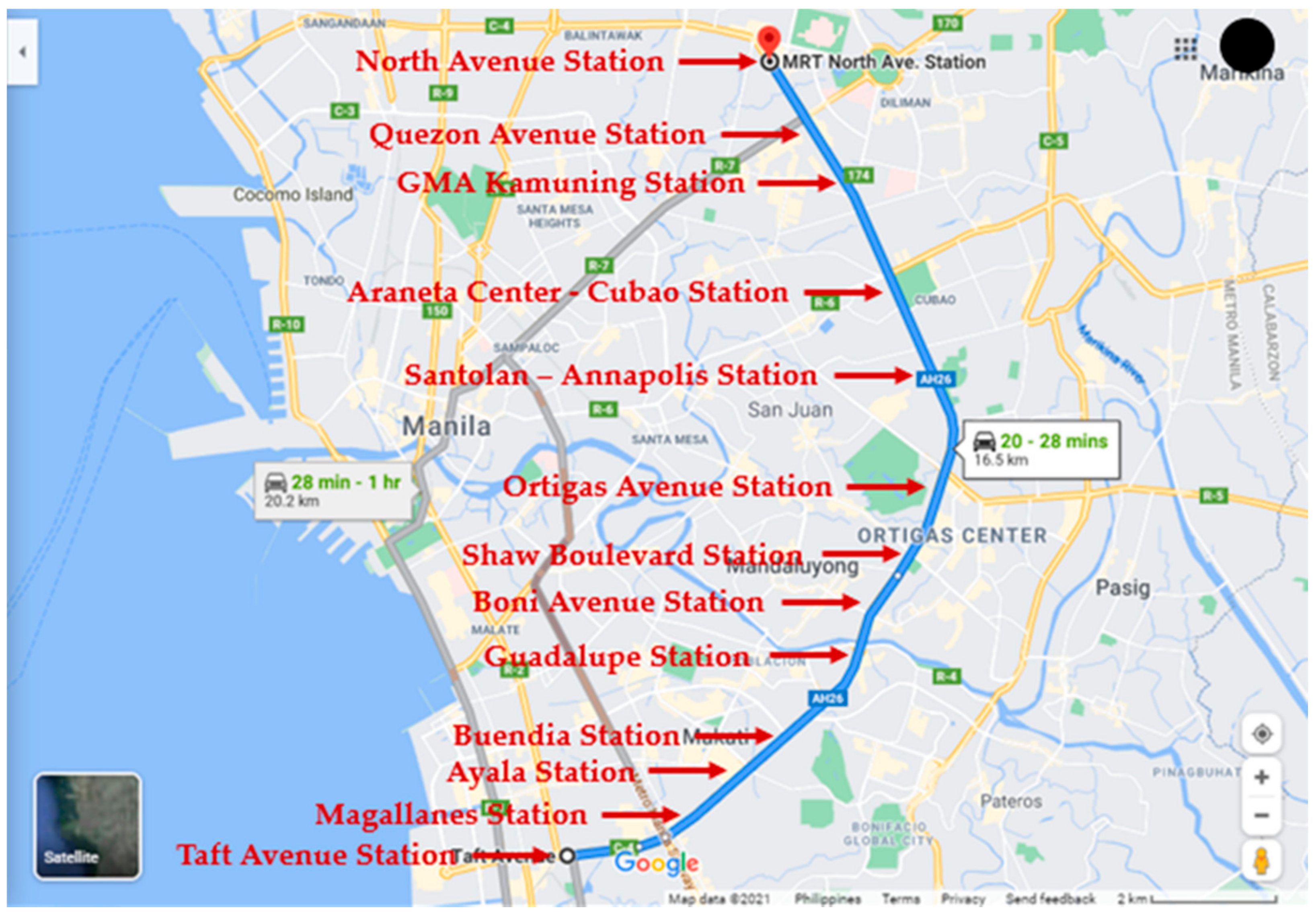
• To begin, identify the specific road or highway that will be studied and determine its starting and end points in Google Maps. The road must be divided into a preferred number of segments. The segment length in kilometers (km) and the actual number of lanes on each side of the road (e.g., northbound and southbound) shall be recorded;
• Decide on the periodicity (e.g., weekly, monthly, and yearly) of the study and select the days of the week from which data collection will be made. Days can be classified according to the identicality of their traffic situations. For example, the modeler can opt to assume that Tuesday, Wednesday, and Thursday have similar traffic conditions;
• Across each road segment, collect and tabulate the average travel time, T_Ave, from Google Maps. By default, this is provided by Google in terms of minutes (min). Convert the unit of time from minutes to hours (hr). Do this at least 24 times, getting at least one data point per hour of the day (i.e., from 0:00 to 23:00). Note that this will be repeated for all the days covered in the study. This tabulation was done manually in the illustrative case study below, but the modeler has the option to automate this using Google Maps’ API service.
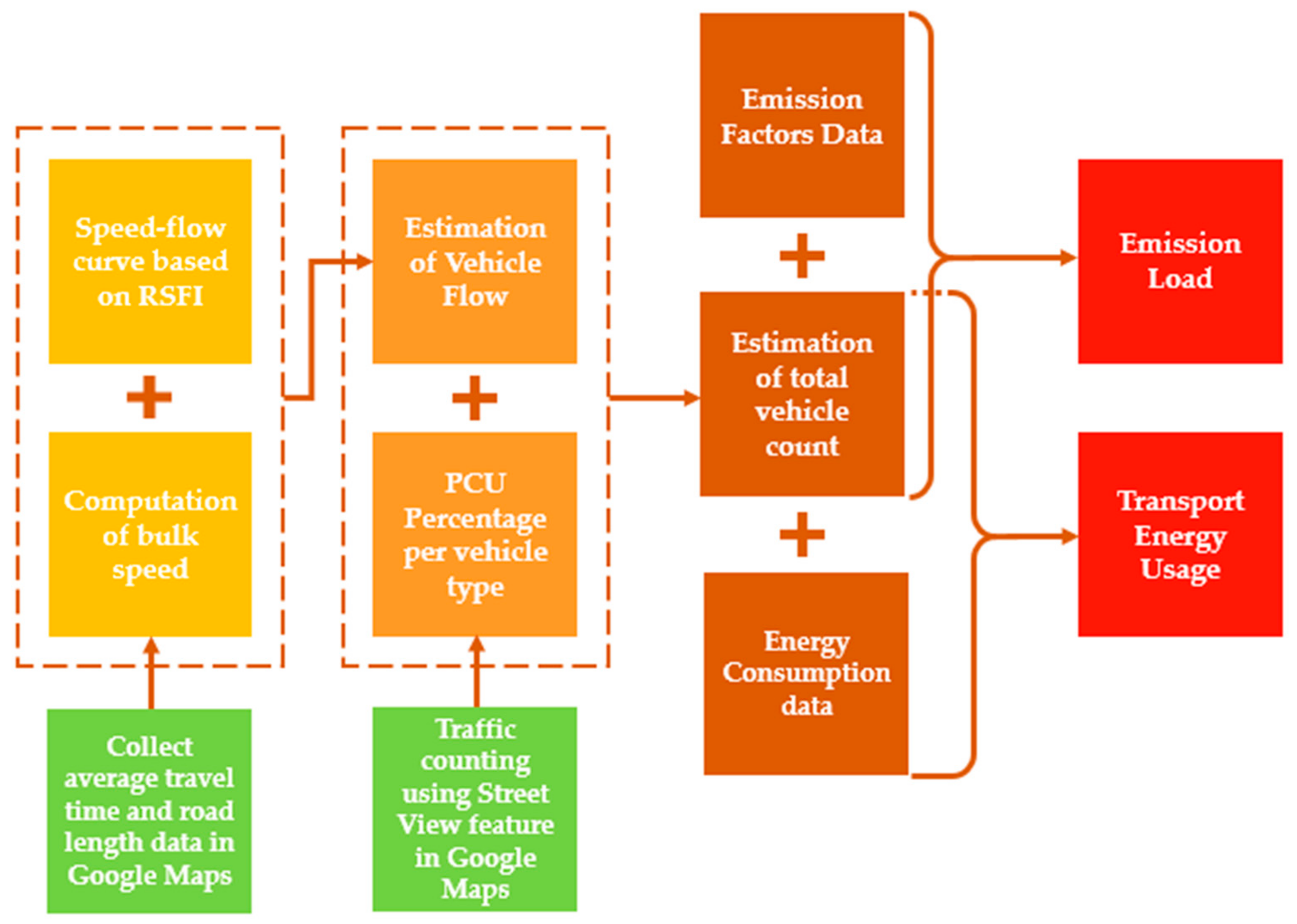
• Calculate the bulk speed, V_B, in terms of kilometers per hour (km/hr) by dividing each segment length, L_S, by the hourly average travel time, T_Ave [41] (see Equation (1) below);

  $${\mathrm{V}}_{\mathrm{B}}=\frac{{\mathrm{L}}_{\mathrm{S}}}{{\mathrm{T}}_{\mathrm{Ave}}}$$

  (1)
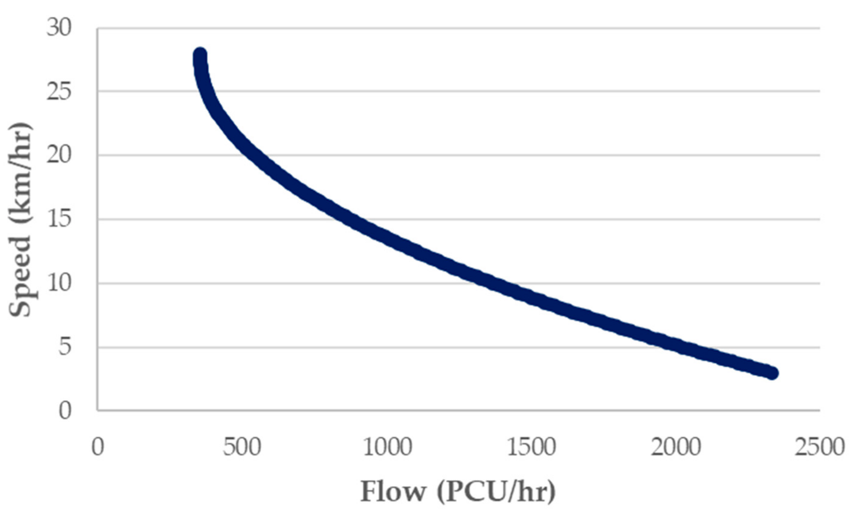
• Through the use of a speed-flow curve, the calculated bulk speed, V_B, from Google Maps is converted to passenger car units per hour (PCU/hr). The unit PCU is used to convert the heterogeneous characteristics of vehicle flow due to the presence of different vehicle types on the road into an equivalent homogenous quantity, using relative weightage factors (i.e., PCEF) [42]. For example, the road space occupied by a bus is equivalent to approximately two passenger cars;
• Assuming that the available speed-flow curve only applies to particular hours of the day, correction factors can be used to adjust the rate of vehicle flow in hours when a significant drop in traffic volume is expected, such as from midnight to the earliest hours of the morning;
• Consolidate the estimated hourly PCU counts for the full 24 h into a total daily PCU count;
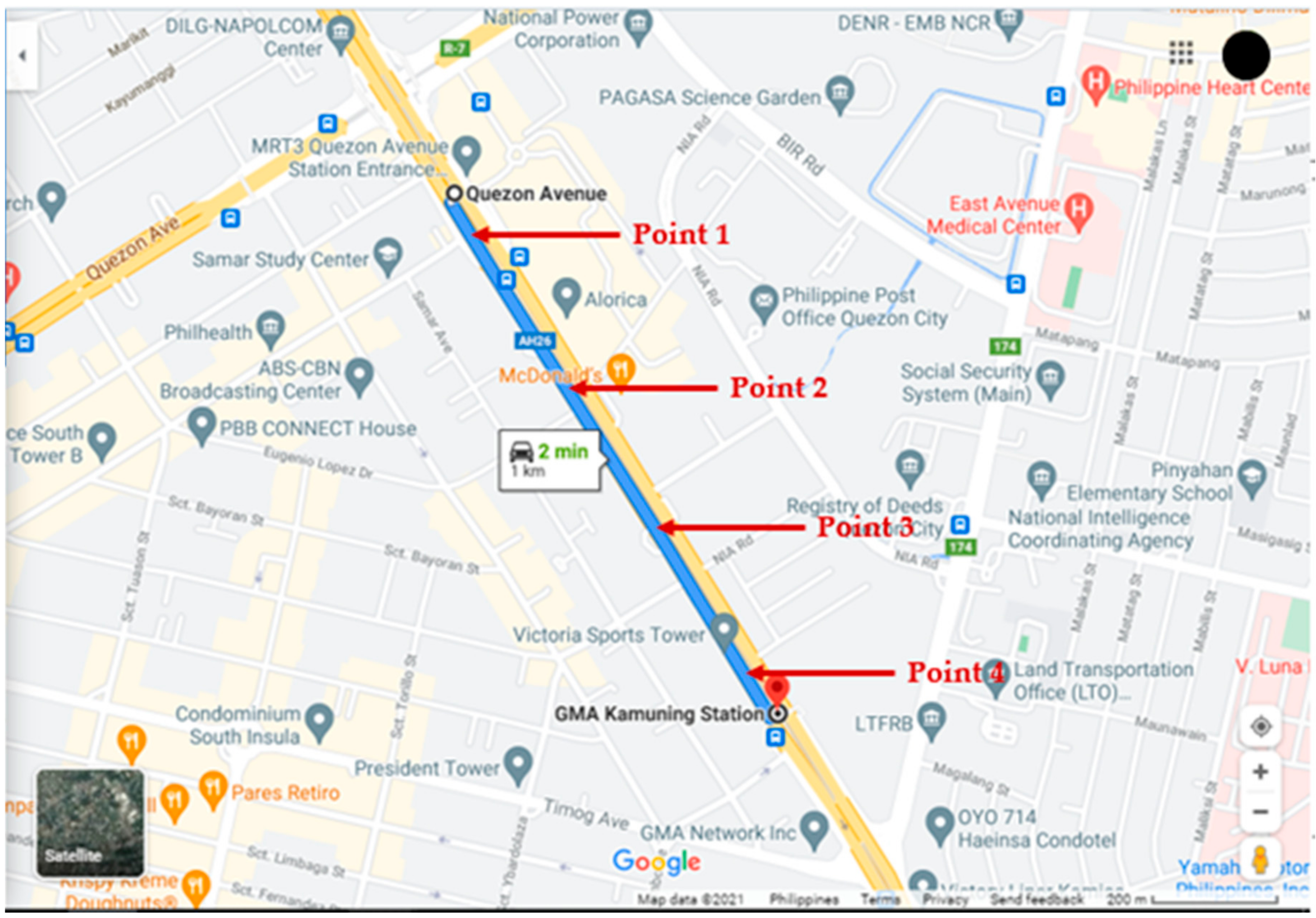
• Within each road segment, assign point coordinates having roughly equidistant spacing with one another as shown in Figure 2 [43]. The modeler has the discretion to determine the distance/spacing between these points, with consideration of road structures, such as the presence of an underpass, flyover, road intersection, etc. The modeler must avoid potential duplication in the counting of vehicles. These points will be used to estimate the modal share;
• Utilizing the Street View feature of Google Maps, perform a classified vehicle count on all of the points identified in the previous step. Count the number of vehicles per variant/category (i.e., motorcycle, tricycle, car, taxi, utility vehicle, jeepney, bus, truck, etc.).
• Multiply the total vehicle count of each category (from Street View counting in Google Maps) with its PCEF, and then divide it by the sum-product of vehicle counts and PCEFs across all categories. This shall generate the PCU mix (i.e., modal share);
• To convert the PCU count into vehicle counts by category, VC, break down the PCU count using the PCU mix obtained in the previous step, and then divide it by the corresponding PCEF for each vehicle category;
• Derive mobile emission factors for each vehicle type with respect to greenhouse gas and air pollutant emissions in terms of grams per kilometer (g_emissions/km), taking into account the variants, fuel type, local emission standards, fuel economy in grams of fuel per kilometer (g_fuel/km), and specific emission factors in grams of emissions per gram of fuel (g_emissions/g_fuel). The emission factors used in this study are shown in the illustrative case study in Section 3. An aggregated emission factor, EF, can be estimated using the PCU mix obtained above;
• Multiply the emission factors, EF, (g_emissions/km) to the segment length, L_S, (km) and to the total vehicle count, VC, in order to obtain the total emissions load, EL. See Equation (2);

  EL = EF × L_S × VC

  (2)
• Derive energy consumption for each vehicle type, EC, in terms of megajoules per kilometers (MJ/km) by taking into account the variants, fuel type, local emission standards, fuel economy in grams of fuel per kilometer (g_fuel/km), and calorific value of fuels, specifically the lower heating values, in terms of megajoules per grams of fuel (MJ/g_fuel).
• Multiply energy consumption, EC, (MJ/km) to the segment length, L_S, (km) and to the total vehicle count, VC, in order to get the total energy use, EU. See Equation (3).

  EU = EC × L_S × VC

  (3)

2.2. Data Collection for the Illustrative Case Study

Epifanio de los Santos Avenue (EDSA) was the subject of the illustrative case study in this paper. It interlinks seven major cities in Metro Manila, making it the main thoroughfare of the economic capital of the Philippines [44]. EDSA will be divided into 12 road segments; furthermore, the authors decided to use the Metro Rail Transit Line 3 (MRT-3) stations as the basis for dividing the avenue into segments. Figure 3 illustrates the whole range of MRT-3 as well as the approximate locations of each station starting from Taft Avenue Station and all the way to North Avenue Station [45]. Currently, MRT-3 has a total of 13 stations spread across five cities: North Avenue Station, Quezon Avenue Station, GMA Kamuning Station, Araneta Center-Cubao Station, and Santolan-Annapolis Station are located in Quezon City; Ortigas Avenue station is located in Pasig City; Shaw Boulevard Station and Boni Avenue Station are located in Mandaluyong City; Guadalupe Station, Buendia Station, Ayala Station, and Magallanes Station are located in Makati City; furthermore, Taft Avenue Station is located in Pasay City.

In the case study, the data collected by the authors was for June 2019. June is the start of the rainy season in the Philippines, thus creating heavier traffic flow [46], while most schools in the country typically start their academic year at this time of the year as well [47]. In the month of June, data were collected for Mondays, Weekdays (i.e., Tuesday, Wednesday, and Thursday), Fridays, Saturdays, and Sundays, assuming that the traffic situations on Tuesdays, Wednesdays, and Thursdays are identical. However, during the actual data collection in Google Maps, it had been observed that the data can have marginal variations despite inputting the same date and time when collected on different occasions. For this reason, the authors collected data on five separate occasions and utilized the average. The dates looked up in Google Maps were 1 June, 2 June, 3 June, 4 June, and 7 June in the year 2019.

As discussed in the previous subsection, the bulk speed can be calculated by dividing average travel time with its segment length. By making use of speed-flow curves, the average speed of all vehicles for a given range can be translated into a rate of vehicle flow. A speed-flow curve is created using what is referred to as the roadside friction index (RSFI), which describes side friction factors or occurrences on the side of the road that affect traffic flow [48]. For example, road segments with schools and wet markets tend to have a higher roadside friction. The speed-flow curve illustrated in Figure 4 was adopted for this case study, with reference to the paper of Pal and Roy [49].

A regression equation was fitted to the speed-flow curve shown on Figure 4. This is a relatively more accurate and convenient approach to obtain vehicle flow rates using the curve [50]. Equation (4) shows the fitted quadratic equation. This will be used to estimate the hourly vehicle flow or PCU_Count, as a function of bulk speed. In an actual study, the authors recommend that speed flow curves for specific road links be utilized to ensure accuracy.

PCU_Count = 3.26V_B² − 180.09V_B + 2843

(4)

The outcome was then multiplied to the average number of lanes assumed for both southbound and northbound directions of the road. An average number of lanes equal to 5 was assumed for EDSA (each way) in this study [51]. However, it is worth noting that the second-degree polynomial equation pertaining to the best fit curve was only applied from 5:00 to 22:00, considering that the traffic is normally heavier during this period. In fact, the average daily traffic volume in terms of PCU according to a transport and environmental survey for some roads in the Philippines had been observed to comparatively drop from 23:00 to 4:00 [52]. Thus, correction factors (or proportionality constants) were introduced for the hours 23:00, 1:00, 2:00, 3:00, and 4:00. Each correction factor was multiplied to the average PCU count value from 5:00 to 22:00. These factors are determined and calibrated by the modeler based on actual on-road observations. The proportionality constants used in the illustrative case study are presented in

Table 1. Correction factors used as constants of proportionality during hours with anticipated significant drops in traffic volume.

Hours with Anticipated Significant Vehicle Volume Drops	Correction Factor
23:00	0.03
0:00	0.02
1:00	0.01
2:00	0.01
3:00	0.01
4:00	0.02

.

Vehicle volume counts need to be normalized as different vehicle categories have different footprints or road space requirements. Expressing volume counts in terms of PCU considers the approximate footprint of each vehicle category by estimating the number of passenger cars occupying the same footprint [53]. These estimates, considered as weightage factors, are called passenger car equivalence factors (PCEFs). Shown in

Table 2. Passenger car equivalence factors for various vehicle types.

Type of Vehicle	PCEF
Tricycle	1
Motorcycle	0.25
Jeepney	1.5
Taxi	1
Car	1
Utility Vehicle	1
Bus	2
Light Truck	2
Heavy Truck	2.2

are the passenger car equivalence factors used in this study. The PCEF values for a car, jeepney, tricycle, bus, light-duty truck, and heavy-duty truck were adopted from a feasibility study relevant to the Philippine road setting [54] while the PCEF values for van, taxi, and motorcycles were adopted from the study of Adnan [55]. Moreover, utility vehicle (UV) as a vehicle type was assigned by the authors to have a PCEF equal to 1. Dividing the PCU count per vehicle type with their respective PCEF generates the estimated vehicle count per category, which will then be used to estimate energy use and emissions. It is worth noting that the jeepney is a unique vehicle category for the Philippines. The Philippine jeepney is the most common mode of public transportation in the country because of its accessibility and affordability [56]. Jeepneys are diesel-powered vehicles that were originally refurbished American military utility vehicles left after the Second World War [57]. Due to most jeepneys being old, the specific engine technology and standards used are not documented, but they are most likely all pre-Euro engines. Fuel-wise, as of writing, all fuel sold in the Philippines is at least Euro 4 quality.

For the classified vehicle count using the Street View feature of Google Maps, four points were identified per road segment, and points were approximately one kilometer from each other.

In the process of estimating emissions, transport activity data is multiplied with emission factors [58,59]. In the context of the transport sector, the greenhouse gas emissions arise from the combustion and evaporation of fuels from diverse forms of transport activities [60]. In particular, the calculation of greenhouse gas emissions on the basis of transport activities and emission factors is referred to as the bottom-up approach in which the transport activities are measured per vehicle kilometer traveled (VKT), and the emission factors are in the units of grams per kilometer [61]. In relation to the current study, the total estimated vehicle count of each road segment together with the respective road lengths determine transport activity.

Emission factors represent the ratio between the quantities of pollutants, expressed in unit weight, that are being discharged to the atmosphere and the activity, expressed in unit weight, volume, distance or time, in connection to the release of these pollutants [62]. However, deriving emission factors relevant to a particular study is an arduous task. With regard to road transport, one needs to take into account the emission standards (i.e., Euro 4 in the Philippines), shares in use of fuel types (diesel or petrol), fuel economies (km/l_fuel or g_emissions/km), fuel properties, specific emission factors (g_emissions/g_fuels), and vehicle variants. In this study, the fuel economy, fuel properties, and specific emission factors were obtained from the databases of Argonne National Laboratory. Specifically, these are from the Greenhouse Gases, Regulated Emissions, and Energy use in Transportation (GREET) Model [63] and the Alternative Fuel Life-Cycle Environmental and Economic Transportation (AFLEET) Tool [64]. The energy use in road transport can also be estimated in the same manner, but the calorific value of the fuel is used as the multiplier instead of the specific emission factor. The calorific value of gasoline and diesel were obtained from the Mechanical Engineer’s Data Handbook authored by James Carvill [65]. For emissions and energy use, the Metro Manila drive cycle utilized in [2] was used.

3. Illustrative Case Study

3.1. Estimation of Monthly Vehicle Count

The estimated vehicle counts in June 2019 are summarized in

Table 3. Estimated Vehicle Count in June 2019.

Monthly Vehicle Count (Southbound EDSA)
Road Segment	Tricycle	Motorcycle	Jeepney	Taxi	Car	Utility Vehicle	Bus	Light Truck	Heavy Truck
North A-Quezon A	0	51,933	0	81,610	59,352	126,124	44,514	3710	0
Quezon A-G Kamuning	0	81832	0	37768	44,063	176,253	0	0	0
G Kamuning-A C Cubao	0	339,941	0	59,837	60,704	105,798	64,173	0	0
A C Cubao-Santolan A	0	45,296	2831	49,543	117,487	134,473	84,931	11,324	0
Santolan A-Ortigas A	0	55,772	2145	23,596	98,674	178,042	39,684	1073	0
Ortigas A-Shaw B	0	16,773	0	16,773	122994	178,900	36,339	2795	0
Shaw B-Boni	0	46,081	0	31,902	106341	233,951	21,268	7089	0
Boni-Guadalupe	0	54,241	0	27,121	57631	149,164	30,511	0	0
Guadalupe-Buendia	0	29,357	1957	25,443	111556	187,884	45,014	0	0
Buendia-Ayala	0	78,073	7435	33,460	74355	66,919	29,742	7435	0
Ayala-Magallanes	0	82,409	0	12,361	61807	86,530	127,735	0	0
Magallanes-Taft A	0	56,876	23,334	30,626	56876	107,919	18,959	16,042	0
Monthly Vehicle Count (Northbound EDSA)
Road Segment	Tricycle	Motorcycle	Jeepney	Taxi	Car	Utility Vehicle	Bus	Light Truck	Heavy Truck
North A-Quezon A	0	86,341	13,283	43,170	149,436	209,211	36,529	6642	0
Quezon A-G Kamuning	0	63,742	0	93,162	112,775	93,162	24,516	4903	0
G Kamuning-A C Cubao	0	275,358	0	76,707	64,906	94,408	51,138	983	0
A C Cubao-Santolan A	0	74,151	0	28,837	148,303	177,139	74,151	8239	0
Santolan A-Ortigas A	0	63,442	1322	26,434	158,605	229,977	34,364	5287	0
Ortigas A-Shaw B	0	71,129	0	35,565	138,308	209,436	59,274	3953	0
Shaw B-Boni	0	93,141	0	37,256	193,732	230,989	67,061	0	0
Boni-Guadalupe	0	95,722	0	0	245,288	233,324	41,879	0	0
Guadalupe-Buendia	0	102,646	0	10,265	164,233	243,784	38,492	0	0
Buendia-Ayala	0	40,424	5775	21,174	94,322	115,496	32,724	0	0
Ayala-Magallanes	0	82,708	0	9543	89,071	213,133	22,268	9543	0
Magallanes-Taft A	3546	35,457	56,732	46,094	109,917	120,555	24,820	0	0

. The data reflects that there were no heavy-duty trucks and tricycles traveling along EDSA both in the southbound and northbound directions, except for the Magallanes Station to Taft Avenue Station road segment, which had an estimated total count of 3546 tricycles. Jeepneys plying EDSA were also limited in number relative to other vehicle types. This is because of the prohibitions by the government for these vehicle types to use most parts of the circumferential road, to accelerate traffic flow [51].

Another assumption made by the authors that can affect the classified vehicle counts involved the assumed variants belonging to each vehicle type. Car as a vehicle type includes the following variants: mini-compact, subcompact, compact, and full-size sedan. On the other hand, utility vehicle considers all variants of sport utility vehicles (SUV), pick-up trucks, and vans such as multi-purpose vehicles (MPV), crossover utility vehicles (CUV), mid-size SUVs, and full-size SUVs. Thus, it is understandable why the majority of the road segments counted more utility vehicles than cars.

The largest shares of vehicle type by road segment are as follows. For southbound EDSA, GMA Kamuning Station to Araneta Center-Cubao Station had a 36.2% share for motorcycles, Magallanes Station to Taft Avenue Station had a 61.9% share for jeepneys; North Avenue Station to Quezon Avenue Station had a 19% share for taxis; Ortigas Avenue Station to Shaw Boulevard Station had a 12.7% share for cars; Shaw Boulevard Station to Boni Avenue Station had a 13.5% share for utility vehicles; Ayala Station to Magallanes Station had a 23.5% share for buses; and lastly, Magallanes Station to Taft Avenue Station had a 32.4% share for light-duty trucks. For northbound EDSA, Magallanes Station to Taft Avenue Station had the highest share of jeepneys at 73.6%. Moreover, it was the only road segment that had tricycles. GMA Kamuning Station to Araneta Center-Cubao Station had the highest share of motorcycles at 25.4%; Quezon Avenue Station to GMA Kamuning Station had a 21.8% share for taxis; Boni Station to Guadalupe Station had a 14.7% share for cars; Guadalupe Station to Buendia Station had an 11.2% share for utility vehicles; Araneta Center-Cubao Station to Santolan-Annapolis Station had a 14.6% share for buses; and finally, Ayala Station to Magallanes Station had a 24.1% share for light-duty trucks.

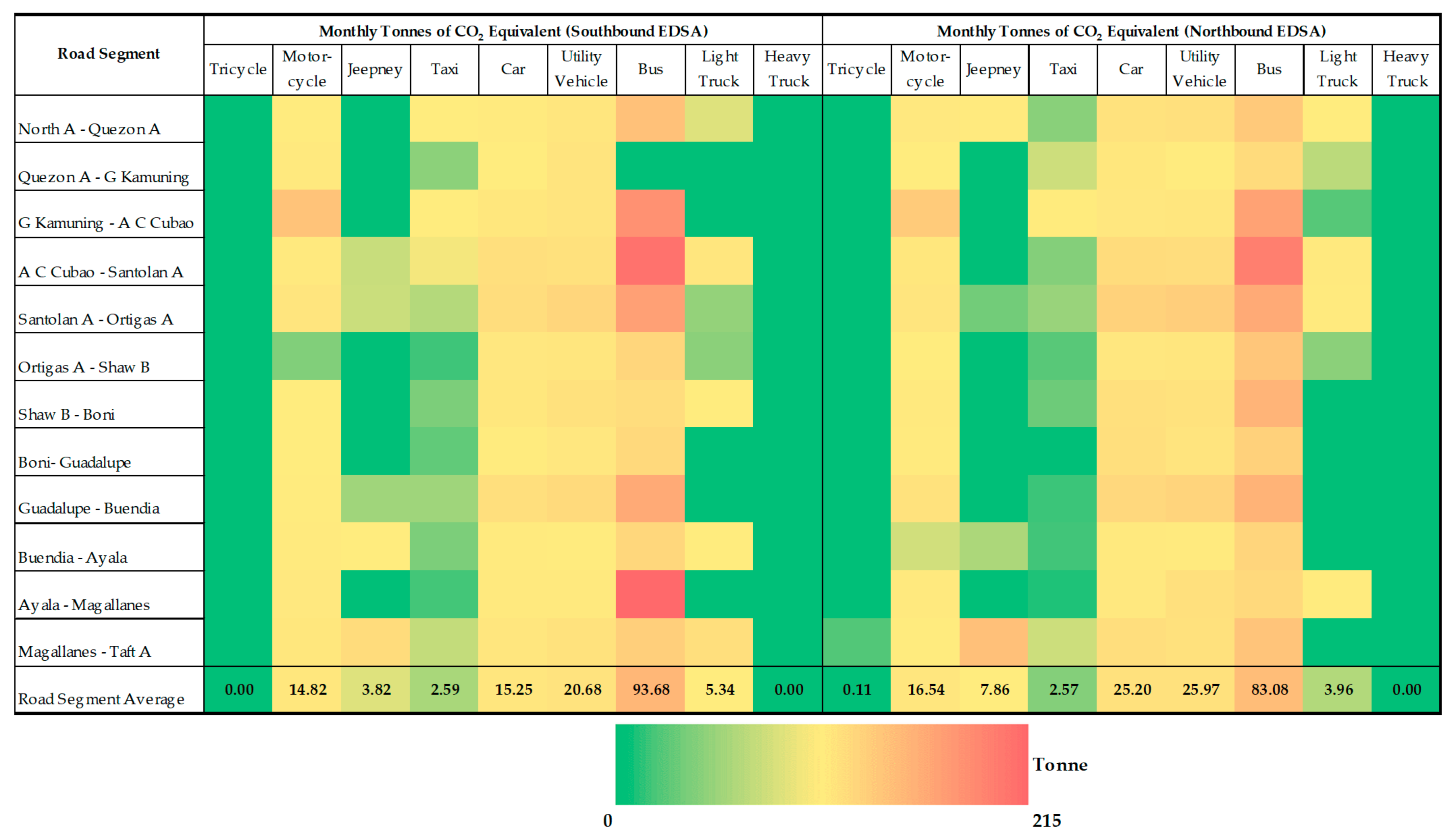
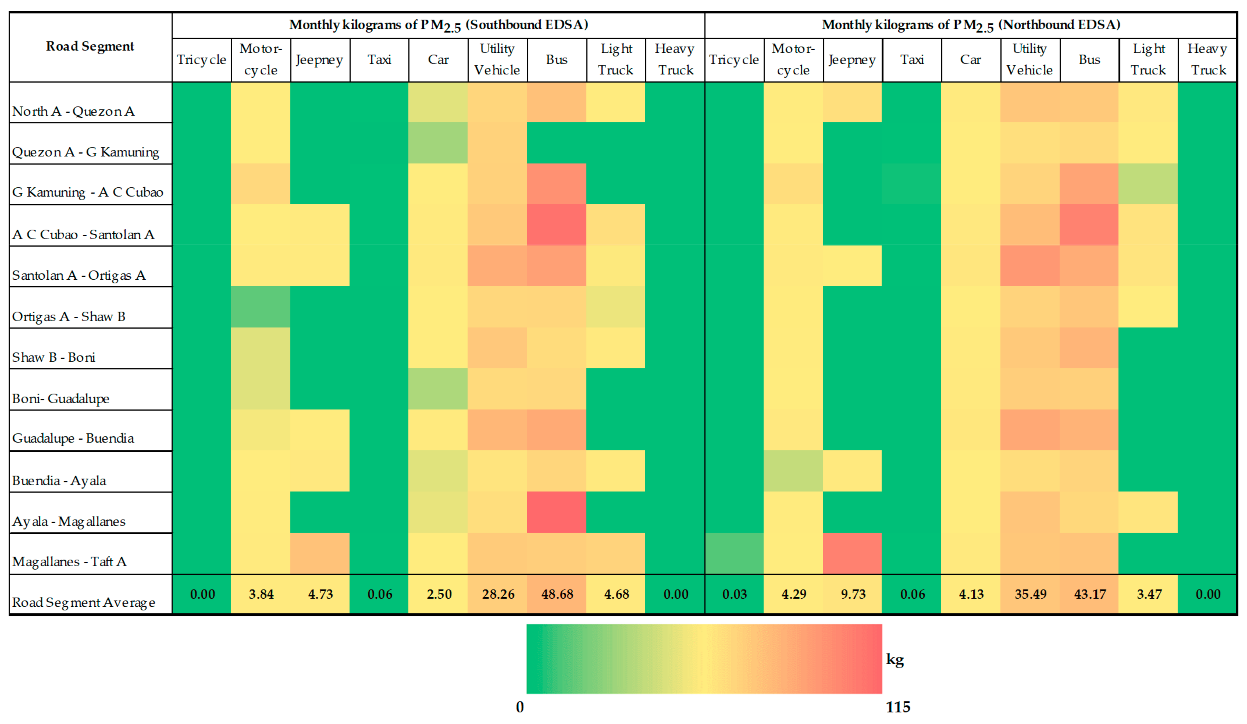
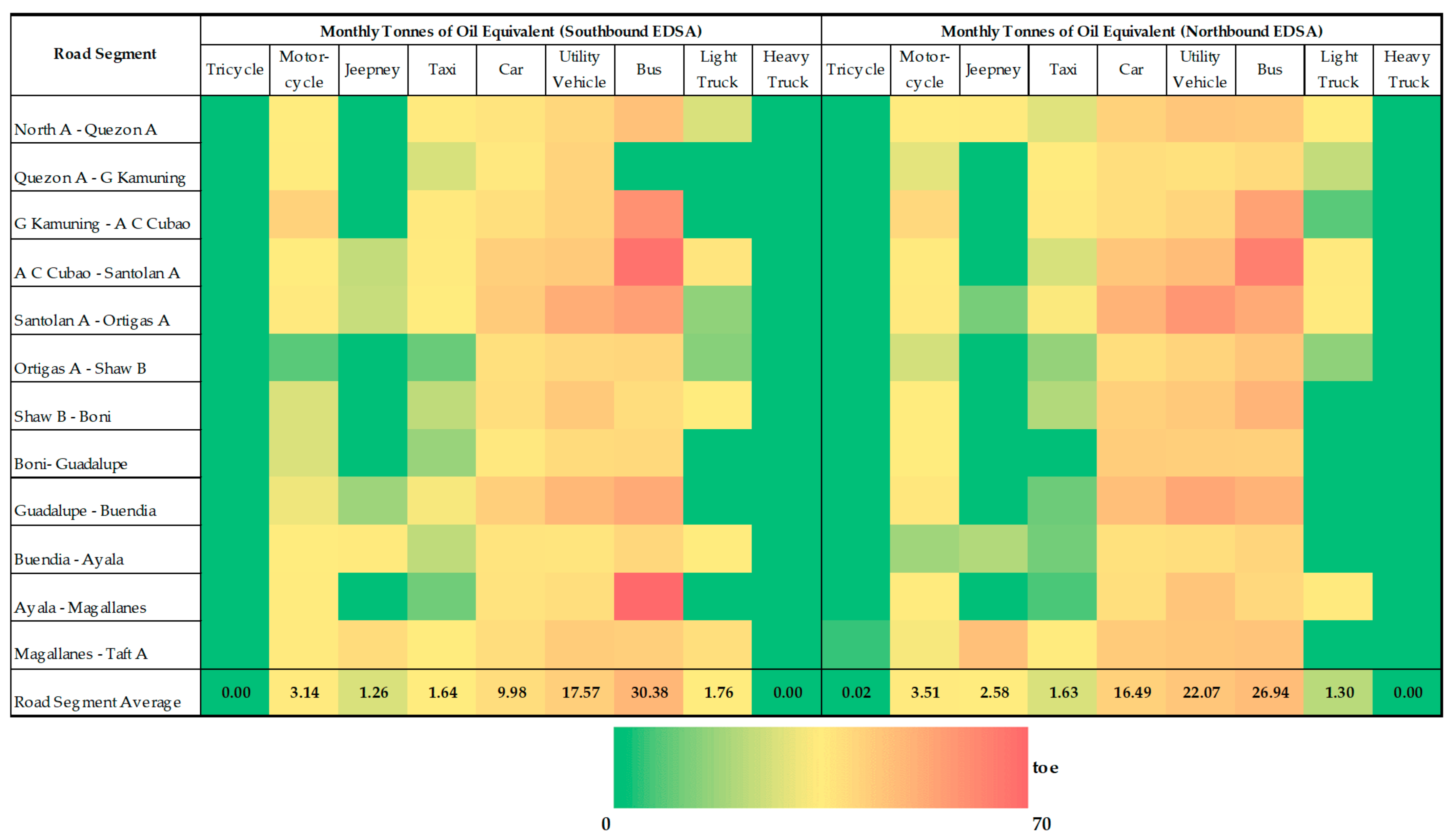
3.2. Estimation of Transport Emissions and Energy Use

The warming effect of greenhouse gases is based on a unit called carbon dioxide equivalent (CO₂eq) [66,67]. Therefore, the authors estimated global warming potential (GWP) using the CO₂eq of each road segment in EDSA for both northbound and southbound directions. The different greenhouse gas emissions are converted to their CO₂eq to measure their heat trapping ability [68]. Shown in Figure 5 are the estimates of CO₂eq emissions in terms of tonnes for the month of June 2019 through the use of clustered heatmaps. In consideration of the effects of air pollutant emissions to human health and environment [5], estimations of fine particulate matter, particularly PM_2.5 [69,70], were also done in the present study. PM_2.5 refers to the infinitesimal particles emitted in the air which measure two and half microns or less in average diameter. Figure 6 shows PM_2.5 emissions in terms of kilograms per road segment and vehicle type. The transport energy use in terms of tonnes of oil equivalent (toe) is shown in Figure 7.

Summarized in

Table 4. Summary of emission factors and energy consumption per vehicle type.

Emission Factors Data (gemissions/km)										CO2 Equivalence(gCO2eq/gemissions)
Types of Emission	Tricycle	Motorcycle	Jeepney	Taxi	Car	Utility Vehicle	Bus	Light Truck	Heavy Truck
PM2.5	0.0562	0.0336	0.8466	0.0011	0.0221	0.1430	0.7539	0.7519	0.6731	-
CH4	4.0906	2.3022	0.2357	0.3000	0.7408	0.3538	1.2873	0.3648	1.0238	30.0000
N2O	0.0021	0.0015	0.0316	0.0039	0.0099	0.0063	0.0222	0.0226	0.0247	265.0000
CO2	66.9747	60.0983	668.7415	41.9204	109.8958	92.4039	1406.2301	842.0852	1672.4363	1.0000
Energy Consumption Data (MJ/km)
	Tricycle	Motorcycle	Jeepney	Taxi	Car	Utility Vehicle	Bus	Light Truck	Heavy Truck
Energy Consumption	1.5285	1.1504	9.4130	1.3812	3.6924	3.7241	19.6944	11.8412	23.3813	-

are the emission factors and energy consumption data which were used in the case study. Firstly, the columns for tricycle and heavy truck in Figure 5, Figure 6 and Figure 7 had the coolest color (i.e., with respect to the heat map). This is because none of these vehicles pass through the majority of the road segments in EDSA, as indicated in Table 3. For some road segments, jeepneys and light trucks also had none, due to a relatively small number of vehicle count, thus resulting in plenty of green tiles on the heatmap. Conversely, the majority of the motorcycle, car, utility vehicle, and bus tiles showed warm colors, indicating substantial contributions to the emission load or energy usage of the road segments.

In Figure 5, Figure 6 and Figure 7, the columns or tiles for buses generally had the warmest colors in comparison to the other vehicle types. However, the vehicle counts for buses based on Table 3 are comparatively smaller compared to motorcycles, cars, and utility vehicles. This observation has something to do with the fact that buses, as indicated in Table 4, have a significantly higher emission factor and energy consumption in comparison to the other vehicle types. For comparison, the emission factors and energy consumption for utility vehicles are 0.14, 0.01, 0.35, 0.01, 92.40 g_emissions/km and 3.72 MJ/km for PM_2.5, CH₄, N₂O, CO₂, and energy consumption, respectively. For buses, these are about 0.75, 0.05, 1.29, 0.02, 1406.23 g_emissions/km and 19.69 MJ/km. The same effect was observed in taxis—despite being greater in vehicle count than jeepneys and light trucks, the estimates of CO₂eq, PM_2.5, and energy use were relatively lower. This observation was also due to the fact that the emission factors and energy consumption for taxis were comparatively lower than jeepneys and light trucks. It is also interesting to note that the road segments with the warmest tiles under the bus column in Figure 5, Figure 6 and Figure 7, namely Araneta Center-Cubao to Santolan-Annapolis and Ayala-Magallanes, are where most provincial bus terminals and major bus stops are located.

3.3. Data Validation

Table 5. Comparison of average daily vehicle counts from MMDA and the proposed method using Google Maps data.

Vehicle Type	MMDA	Percentage Share	Google Maps	Percentage Share
Tricycle	9	0%	118	0%
Motorcycle	110,167	27%	70,299	19%
Jeepney	2166	1%	3827	1%
Taxi	18,913	5%	29,745	8%
Car	255,732	63%	91,817	25%
Utility Vehicle	6285	2%	136,514	37%
Bus	11,313	3%	35,496	10%
Light Truck	1297	0%	3038	1%
Heavy Truck	0	0%	0	0%
Total	405,882	100%	370,854	100%

shows the comparison between the annual average daily traffic (AADT) reported by the Metropolitan Manila Development Authority (MMDA) in 2019 [71] and the average daily vehicle count estimated using crowdsourced data from Google Maps. The total number of vehicles from both sources were within close range. The MMDA reported a total of 405,882 vehicles while the authors estimated 370,855 vehicles in total (i.e., 8.63% error). Having said that, considerable discrepancies on the individual percentage share for each vehicle type were observed especially in cars, utility vehicles, and buses. One possible cause for the discrepancies in car and utility vehicle percentage shares is the assignment of vehicle variants belonging to each type. This assumption might have been different with how the MMDA did it in their actual survey. Note that if the vehicle shares of cars and utility vehicles were to be aggregated in both reports, the percentage error will only be 4.63%. It is important to take note also that the PCEF values for cars and utility vehicles (see Table 2) are the same. In fact, the two can theoretically be classified into one vehicle type in as much as PCU count is concerned. Another possible reason for the discrepancies in the percentage shares is the timing when data collection took place. It is important to note that the Google Maps Street View feature does not specify the time of data collection. In this regard, the authors assumed a constant PCU percentage share (modal share) throughout the whole day. The same is true with the survey performed by MMDA—there was also no information regarding the time of data collection in the survey report.

4. Limitations and Future Work

The study demonstrated a convenient and cost-effective way to estimate emission load and energy use in road transport. One major advantage of using the proposed method is the availability and accessibility of the data. Furthermore, it makes multi-regional or multi-locality studies for benchmarking purposes easier to do. For instance, researchers can easily conduct studies on a city aside from their own. Most importantly, the gathering of data according to the said method can be used as an alternative to conducting an actual survey, which is more laborious and resource-intensive. It is important to take note that the proposed methodology in this work provides an alternative only for vehicle data and traffic flow collection. It is not meant to replace the whole emissions modeling approach, as it is rather more complex than the simplified approach used in this study. If desired by the modeler, the proposed approach to collect vehicle and traffic data in Google Maps can be coupled to other more sophisticated emissions models for more accurate estimates.

Despite the advantages, there are also some disadvantages. Aside from the Google Maps data, the methodology is also highly dependent on data from various references and assumptions. Therefore, these can become sources of inaccuracies in the results. In some countries, data concerning the transportation sector can be more accessible. Another major assumption used in the current case study is the speed-flow curve adopted. In vehicle flow analysis, speed-flow curves and PCEFs are derived based on the dynamic characteristics and positions of vehicles for specific roads. The illustrative case study used a speed-flow curve that had been modeled from a specific highway in India. On the other hand, the PCEFs used, although relevant to Philippine roads, were taken from a feasibility study published in 1987.

To address these limitations for the Philippines, the authors propose the following for future work. First, research on speed-flow curve modeling, particularly for the major thoroughfare, EDSA, is needed. Relevant literature in developing speed-flow curves includes [49,72,73]. Second, a future research study should develop updated values of PCEFs considering the current traffic characteristics of Philippine highways. Relevant literature in measuring PCEFs includes [55,74,75]. To reduce uncertainty in data, a probabilistic analysis could be used to improve the robustness of the results. For example, a Monte Carlo approach can be used to explore the robustness of the data collected from Google Maps and Google Street View.

5. Conclusions

A novel method for estimating emissions and energy use in road transport using crowdsourced data from Google Maps was introduced and demonstrated by the authors. Two particular sets of data are utilized from Google Maps. The first is the travel time and road length data which will be converted into bulk speed or the average speed of all vehicles. Subsequently, the rate of vehicle flow in terms of PCU/hr is determined using the calculated bulk speed. The second dataset collected from Google Maps is the classified vehicle count using Google Street View. After establishing the rate of vehicle flows and PCU mix, PCEF values are utilized to break down the PCU into different types of vehicles. Finally, emissions and energy use in road transport are estimated by multiplying the vehicle count with the assumed emission factors and energy consumption data.

An illustrative case study was performed to demonstrate the actual use of this methodology, which was also validated using government-reported daily traffic data (AADT). The average daily vehicle count estimated using the proposed method had about an 8.63% error when compared to the AADT survey conducted by MMDA in the same year. However, this can be further reduced to 4.63% if cars and utility vehicles were combined. This means that the proposed method can accurately estimate average traffic flow, given proper assumptions on the data.

Furthermore, CO₂eq, PM_2.5, and energy use were estimated in the case study. The results were illustrated through clustered heatmaps showing the share of each road segment and vehicle type. Results indicated that buses, despite having less vehicle counts, had the largest contributions to CO₂eq, PM_2.5, and energy use. On the contrary, taxis, despite being greater in vehicle count than jeepneys and light-duty trucks, had one of the least contributions to CO₂eq, PM_2.5, and energy use. Based on the average values in southbound and northbound EDSA, buses produced 88.38 tonnes of CO₂eq and 43.93 kg of PM_2.5 monthly per road segment while consuming 28.66 toe. Furthermore, taxis discharged 2.58 tonnes of CO₂eq. and 0.06 kg of PM_2.5 monthly per road segment while consuming 1.64 toe.

Since the novelty of this study is using crowdsourced data in Google Maps, this study can give rise to future works which can improve the methodology in such a way that possible inaccuracies and uncertainties can be mitigated and considered better. While the proposed methodology demonstrated promising results in the illustrative case study, this research is an evolving work that shows great potential to streamline methodologies in estimating emission load and energy use in road transport. While much of the data collection work was done manually in this paper, future research can easily automate plenty of these steps.

References

1. Stern, N. The Economics of Climate Change. Am. Econ. Rev. 2008, 98, 1–37. [Google Scholar] [CrossRef] [Green Version]
2. Lopez, N.S.; Soliman, J.; Biona, J.B.M.; Fulton, L. Cost-benefit analysis of alternative vehicles in the Philippines using immediate and distant future scenarios. Transp. Res. Part D Transp. Environ. 2020, 82, 102308. [Google Scholar] [CrossRef]
3. International Energy Agency. Global Energy & CO2 Status Report; International Energy Agency: Paris, France, 2019. [Google Scholar]
4. United Nations. Paris Agreement; United Nations: Paris, France, 2015. [Google Scholar]
5. Manisalidis, I.; Stavropoulou, E.; Stavropoulos, A.; Bezirtzoglou, E. Environmental and Health Impacts of Air Pollution: A Review. Front. Public Health 2020, 8, 1–13. [Google Scholar] [CrossRef] [PubMed] [Green Version]
6. Ritchie, H.; Roser, M. Outdoor Air Pollution. Available online: https://ourworldindata.org/outdoor-air-pollution (accessed on 20 May 2021).
7. Stanaway, J.D.; Afshin, A.; Gakidou, E.; Lim, S.S.; Abate, D.; Abate, K.H.; Abbafati, C.; Abbasi, N.; Abbastabar, H.; Abd-Allah, F.; et al. Global, regional, and national comparative risk assessment of 84 behavioural, environmental and occupational, and metabolic risks or clusters of risks for 195 countries and territories, 1990–2017: A systematic analysis for the Global Burden of Disease Stu. Lancet 2018, 392, 1923–1994. [Google Scholar] [CrossRef] [Green Version]
8. Lopez, N.S.; Chiu, A.S.F.; Biona, J.B.M. Decomposing drivers of transportation energy consumption and carbon dioxide emissions for the Philippines: The case of developing countries. Front. Energy 2018, 12, 389–399. [Google Scholar] [CrossRef]
9. International Energy Agency. Clean Energy Transitions Programme; International Energy Agency: Paris, France, 2021. [Google Scholar]
10. Hall, D.; Lutsey, N. Estimating the infrastructure needs and costs for the launch of zero-emission trucks. Int. Counc. Clean Transp. 2019, 1–31. [Google Scholar] [CrossRef]
11. Anenberg, S.C.; Miller, J.; Henze, D.K.; Minjares, R.; Achakulwisut, P. The global burden of transportation tailpipe emissions on air pollution-related mortality in 2010 and 2015. Environ. Res. Lett. 2019, 14, 094012. [Google Scholar] [CrossRef]
12. Acaravci, A.; Ozturk, I. On the relationship between energy consumption, CO2 emissions and economic growth in Europe. Energy 2010, 35, 5412–5420. [Google Scholar] [CrossRef]
13. Zou, S.; Zhang, T. CO2 Emissions, Energy Consumption, and Economic Growth Nexus: Evidence from 30 Provinces in China. Math. Probl. Eng. 2020, 2020, 1–10. [Google Scholar] [CrossRef]
14. International Energy Agency. Energy Efficiency Indicators Highlights; International Energy Agency: Paris, France, 2020. [Google Scholar]
15. Song, M.; Wu, N.; Wu, K. Energy Consumption and Energy Efficiency of the Transportation Sector in Shanghai. Sustainability 2014, 6, 702–717. [Google Scholar] [CrossRef] [Green Version]
16. Furfari, S. Energy efficiency of engines and appliances for transport on land, water, and in air. Ambio 2016, 45, 63–68. [Google Scholar] [CrossRef] [PubMed] [Green Version]
17. Engeset, P.; Keitheile, O.B. Traffic Data Collection and Analysis; Ministry of Works and Transport: Gaborone, Botswana, 2004. [Google Scholar]
18. Paľo, J.; Caban, J.; Kiktová, M.; Černický, Ľ. The comparison of automatic traffic counting and manual traffic counting. IOP Conf. Ser. Mater. Sci. Eng. 2019, 710, 012041. [Google Scholar] [CrossRef]
19. Wardrop, J.G.; Charlesworth, G. A Method of Estimating Speed and Flow of Traffic from a Moving Vehicle. Proc. Inst. Civ. Eng. 1954, 3, 158–171. [Google Scholar] [CrossRef]
20. Mortimer, W.J. Moving Vehicle Method of Estimating Traffic Volumes and Speeds. Highw. Res. Board Bull. 1957, 156, 1–13. [Google Scholar]
21. Venkatcharyulu, S.; Mallikarjunareddy, V. Traffic volume Analysis of Newly Developing semi-urban Road. E3S Web Conf. 2020, 184, 01116. [Google Scholar] [CrossRef]
22. Zhao, N.; Qi, T.; Yu, L.; Zhang, J.; Jiang, P. A Practical Method for Estimating Traffic Flow Characteristic Parameters of Tolled Expressway Using Toll Data. Procedia Soc. Behav. Sci. 2014, 138, 632–640. [Google Scholar] [CrossRef] [Green Version]
23. Seo, T.; Kusakabe, T. Probe vehicle-based traffic flow estimation method without fundamental diagram. Transp. Res. Procedia 2015, 9, 149–163. [Google Scholar] [CrossRef] [Green Version]
24. Aksoy, A.; Küçükoğlu, İ.; Ene, S.; Öztürk, N. Integrated Emission and Fuel Consumption Calculation Model for Green Supply Chain Management. Procedia Soc. Behav. Sci. 2014, 109, 1106–1109. [Google Scholar] [CrossRef] [Green Version]
25. Jabali, O.; Van Woensel, T.; de Kok, A.G. Analysis of Travel Times and CO 2 Emissions in Time-Dependent Vehicle Routing. Prod. Oper. Manag. 2012, 21, 1060–1074. [Google Scholar] [CrossRef]
26. Bharadwaj, S.; Ballare, S.; Rohit Chandel, M.K. Impact of congestion on greenhouse gas emissions for road transport in Mumbai metropolitan region. Transp. Res. Procedia 2017, 25, 3538–3551. [Google Scholar] [CrossRef]
27. Nesamani, K.S.; Saphores, J.; McNally, M.G.; Jayakrishnan, R. Estimating impacts of emission specific characteristics on vehicle operation for quantifying air pollutant emissions and energy use. J. Traffic Transp. Eng. 2017, 4, 215–229. [Google Scholar] [CrossRef]
28. de Maes, A.S.; Hoinaski, L.; Meirelles, T.B.; Carlson, R.C. A methodology for high resolution vehicular emissions inventories in metropolitan areas: Evaluating the effect of automotive technologies improvement. Transp. Res. Part D Transp. Environ. 2019, 77, 303–319. [Google Scholar] [CrossRef]
29. Iqbal, A.; Allan, A.; Zito, R. Meso-scale on-road vehicle emission inventory approach: A study on Dhaka City of Bangladesh supporting the ‘cause-effect’ analysis of the transport system. Environ. Monit. Assess. 2016, 188, 149. [Google Scholar] [CrossRef] [PubMed]
30. Zhang, L.; Lin, J.; Qiu, R. Characterizing the toxic gaseous emissions of gasoline and diesel vehicles based on a real-world on-road investigation. J. Clean. Prod. 2021, 286, 124957. [Google Scholar] [CrossRef]
31. Iqbal, A.; Afroze, S.; Rahman, M.M. Probabilistic Health Risk Assessment of Vehicular Emissions as an Urban Health Indicator in Dhaka City. Sustainability 2019, 11, 6427. [Google Scholar] [CrossRef] [Green Version]
32. Chatzimilioudis, G.; Zeinalipour-Yazti, D. Crowdsourcing for Mobile Data Management. In Proceedings of the 2013 IEEE 14th International Conference on Mobile Data Management, Milan, Italy, 3–6 June 2013; Volume 2, pp. 3–4. [Google Scholar]
33. Brabham, D.C. Crowdsourcing as a Model for Problem Solving. Converg. Int. J. Res. N. Media Technol. 2008, 14, 75–90. [Google Scholar] [CrossRef]
34. Misra, A.; Gooze, A.; Watkins, K.; Asad, M.; Le Dantec, C.A. Crowdsourcing and Its Application to Transportation Data Collection and Management. Transp. Res. Rec. J. Transp. Res. Board 2014, 2414, 1–8. [Google Scholar] [CrossRef] [Green Version]
35. Chandra, S.; Naik, R.T.; Jimenez, J. A Framework for Smart Freight Mobility with Crowdsourcing. Transp. Res. Procedia 2020, 48, 494–502. [Google Scholar] [CrossRef]
36. Nair, D.J.; Gilles, F.; Chand, S.; Saxena, N.; Dixit, V. Characterizing multicity urban traffic conditions using crowdsourced data. PLoS ONE 2019, 14, e0212845. [Google Scholar] [CrossRef] [Green Version]
37. Ferster, C.; Nelson, T.; Laberee, K.; Vanlaar, W.; Winters, M. Promoting Crowdsourcing for Urban Research: Cycling Safety Citizen Science in Four Cities. Urban Sci. 2017, 1, 21. [Google Scholar] [CrossRef] [Green Version]
38. Wang, X.; Zheng, X.; Zhang, Q.; Wang, T.; Shen, D. Crowdsourcing in ITS: The State of the Work and the Networking. IEEE Trans. Intell. Transp. Syst. 2016, 17, 1596–1605. [Google Scholar] [CrossRef]
39. Zheng, X.; Chen, W.; Wang, P.; Shen, D.; Chen, S.; Wang, X.; Zhang, Q.; Yang, L. Big Data for Social Transportation. IEEE Trans. Intell. Transp. Syst. 2016, 17, 620–630. [Google Scholar] [CrossRef]
40. Linton, C.; Grant-Muller, S.; Gale, W.F. Approaches and Techniques for Modelling CO 2 Emissions from Road Transport. Transp. Rev. 2015, 35, 533–553. [Google Scholar] [CrossRef]
41. Jiménez-Meza, A.; Arámburo-Lizárraga, J.; de la Fuente, E. Framework for Estimating Travel Time, Distance, Speed, and Street Segment Level of Service (LOS), based on GPS Data. Procedia Technol. 2013, 7, 61–70. [Google Scholar] [CrossRef] [Green Version]
42. Sharma, M.; Biswas, S. Estimation of Passenger Car Unit on urban roads: A literature review. Int. J. Transp. Sci. Technol. 2020. [Google Scholar] [CrossRef]
43. Google Maps. Available online: https://www.google.com/maps/dir/Quezon+Avenue/GMA+Kamuning+Station/@14.6389009,-121.0371689,16z/data=!4m18!4m17!1m5!1m1!1s0x3397b7aa16a4f333:0x5eefaaf26ee44220!2m2!1d121.0385078!2d14.6427595!1m5!1m1!1s0x3397b7af0a4f1251:0x867338649729026b!2m2!1d121.0433426 (accessed on 30 April 2021).
44. Ganiron, T.U.J. Exploring the Emerging Impact of Metro Rail Transit (MRT-3) in Metro Manila. Int. J. Adv. Sci. Technol. 2015, 74, 11–24. [Google Scholar] [CrossRef]
45. Google Maps. Available online: https://www.google.com/maps/dir/Taft+Avenue/MRT+North+Ave.+Station,+Bagong+Pag-asa,+Quezon+City,+Metro+Manila/@14.5950342,120.9740679,12z/data=!4m18!4m17!1m5!1m1!1s0x3397c945008b5cb5:0x23dd98e8b1d43815!2m2!1d121.0021747!2d14.537669!1m5!1m1!1s0x3397b6fd9e1 (accessed on 20 April 2021).
46. Cruz, F.T.; Narisma, G.T.; Villafuerte, M.Q.; Cheng Chua, K.U.; Olaguera, L.M. A climatological analysis of the southwest monsoon rainfall in the Philippines. Atmos. Res. 2013, 122, 609–616. [Google Scholar] [CrossRef]
47. Villafuerte, M.Q.; Juanillo, E.L.; Hilario, F.D. Climatic insights on academic calendar shift in the Philippines. Philipp. J. Sci. 2017, 146, 267–276. [Google Scholar]
48. Salini, S.; George, S.; Ashalatha, R. Effect of Side Frictions on Traffic Characteristics of Urban Arterials. Transp. Res. Procedia 2016, 17, 636–643. [Google Scholar] [CrossRef]
49. Pal, S.; Roy, S.K. Impact of Roadside Friction on Travel Speed and LOS of Rural Highways in India. Transp. Dev. Econ. 2016, 2, 9. [Google Scholar] [CrossRef] [Green Version]
50. Srikanth, S.; Mehar, A. Estimation of Equivalency Units for Vehicle Types under Mixed Traffic Conditions: Multiple Non-Linear Regression Approach. Int. J. Technol. 2017, 8, 820. [Google Scholar] [CrossRef] [Green Version]
51. Boquet, Y. Battling Congestion in Manila: The EDSA Problem. Transp. Commun. Bull. Asia Pacific 2013, 45–59. [Google Scholar]
52. Japan International Cooperation Agency; Department of Public Works and Highways. Transport and Environmental Surveys. In The Feasibility Study and Implementation Support for Cavite-Laguna East-West National Road Project; Japan International Cooperation Agency: Tokyo, Japan, 2006; pp. 1–84. [Google Scholar]
53. Al-Kaisy, A.; Jung, Y.; Rakha, H. Developing Passenger Car Equivalency Factors for Heavy Vehicles during Congestion. J. Transp. Eng. 2005, 131, 514–523. [Google Scholar] [CrossRef]
54. Japan International Cooperation Agency; Department of Public Works and Highways. Feasibility Study of the Road Improvement Project on the Pan-Philippine Highway (Philippine-Japan Friendship Highway); Japan International Cooperation Agency: Tokyo, Japan, 1987. [Google Scholar]
55. Adnan, M. Passenger Car Equivalent Factors in Heterogenous Traffic Environment-are We Using the Right Numbers? Procedia Eng. 2014, 77, 106–113. [Google Scholar] [CrossRef] [Green Version]
56. Coz, M.C.; Flores, P.J.; Hernandez, K.L.; Portus, A.J. An Ergonomic Study on the UP-Diliman Jeepney Driver’s Workspace and Driving Conditions. Procedia Manuf. 2015, 3, 2597–2604. [Google Scholar] [CrossRef] [Green Version]
57. Agaton, C.B.; Guno, C.S.; Villanueva, R.O.; Villanueva, R.O. Diesel or Electric Jeepney? A Case Study of Transport Investment in the Philippines Using the Real Options Approach. World Electr. Veh. J. 2019, 10, 51. [Google Scholar] [CrossRef] [Green Version]
58. Kim, H.; Tae, S.; Yang, J. Calculation Methods of Emission Factors and Emissions of Fugitive Particulate Matter in South Korean Construction Sites. Sustainability 2020, 12, 9802. [Google Scholar] [CrossRef]
59. Olaguer, E.P. Emission Inventories. In Atmospheric Impacts of the Oil and Gas Industry; Elsevier: Amsterdam, The Netherlands, 2017; pp. 67–77. ISBN 9780128018835. [Google Scholar]
60. Waldron, C.D.; Harnisch, J.; Lucon, O.; Mckibbon, R.S.; Saile, S.B.; Wagner, F.; Walsh, M.P.; Kapshe, M. Mobile Combustion. In 2006 IPCC Guidelines for National Greenhouse Gas Inventories Volume 2 Energy; Institute for Global Environmental Strategies: Kanagawa, Japan, 2006; pp. 1–78. [Google Scholar]
61. Bongardt, D.; Eichhorst, U.; Dünnebeil, F.; Reinhard, C. Monitoring Greenhouse Gas Emissions of Transport Activities in Chinese Cities; Deutsche Gesellschaft für Internationale Zusammenarbeit: Bonn, Germany, 2016. [Google Scholar]
62. Cheremisinoff, N.P. Pollution Management and Responsible Care. In Waste; Elsevier: Cambridge, UK, 2011; pp. 487–502. ISBN 9780123814753. [Google Scholar]
63. Argonne National Laboratory The Greenhouse gases, Regulated Emissions, and Energy use in Technologies (GREET) Model. Available online: https://greet.es.anl.gov/greet.models (accessed on 6 January 2021).
64. Argonne National Laboratory Alternative Fuel Life-Cycle Environmental and Economic Transportation (AFLEET) Tool. Available online: https://greet.es.anl.gov/afleet (accessed on 6 January 2021).
65. Carvill, J. Mechanical Engineer’s Data Handbook, 1st ed.; Elsevier: Oxford, UK, 1993; ISBN 9780080511351. [Google Scholar]
66. Yoro, K.O.; Daramola, M.O. CO2 emission sources, greenhouse gases, and the global warming effect. In Advances in Carbon Capture; Elsevier: Cambridge, UK, 2020; pp. 3–28. ISBN 9780128196571. [Google Scholar]
67. Dincer, I.; Abu-Rayash, A. Sustainability modeling. In Energy Sustainability; Elsevier: Amsterdam, The Netherlands, 2020; pp. 119–164. ISBN 9780128195567. [Google Scholar]
68. Vallero, D.A. Air pollution biogeochemistry. In Air Pollution Calculations; Elsevier: Amsterdam, The Netherlands, 2019; pp. 175–206. ISBN 9780128149348. [Google Scholar]
69. Myong, J.-P. Health Effects of Particulate Matter. Korean J. Med. 2016, 91, 106–113. [Google Scholar] [CrossRef]
70. Xing, Y.F.; Xu, Y.H.; Shi, M.H.; Lian, Y.X. The impact of PM2.5 on the human respiratory system. J. Thorac. Dis. 2016, 8, E69–E74. [Google Scholar] [CrossRef]
71. Metropolitan Manila Developement Authority Metropolitan Manila Annual Average Daily Traffic (AADT) 2019. Available online: https://mmda.gov.ph/2-uncategorised/3345-freedom-of-information-foi.html (accessed on 30 April 2021).
72. Bains, M.S.; Ponnu, B.; Arkatkar, S.S. Modeling of Traffic Flow on Indian Expressways using Simulation Technique. Procedia Soc. Behav. Sci. 2012, 43, 475–493. [Google Scholar] [CrossRef] [Green Version]
73. Bharadwaj, N.; Kumar, P.; Arkatkar, S.S.; Joshi, G. Deriving capacity and level-of-service thresholds for intercity expressways in India. Transp. Lett. 2020, 12, 182–196. [Google Scholar] [CrossRef]
74. Ahmed, U. Passenger Car Equivalent Factors for Level Freeway Segments Operating under Moderate and Congested Conditions; Marquette University: Milwaukee, WI, USA, 2010. [Google Scholar]
75. Lu, P.; Zheng, Z.; Tolliver, D.; Pan, D. Measuring Passenger Car Equivalents (PCE) for Heavy Vehicle on Two Lane Highway Segments Operating Under Various Traffic Conditions. J. Adv. Transp. 2020, 2020, 1–9. [Google Scholar] [CrossRef] [Green Version]
Figure 1. The general framework of the proposed method for estimating road transport energy use and emissions using crowdsourced data in Google Maps and Google Street View.
Sustainability 13 06682 g001
Figure 2. Assigning of point coordinates in Google Maps. Data Source: Google Maps.
Sustainability 13 06682 g002
Figure 3. The approximate locations of the 13 MRT-3 stations which will be used as the basis for dividing EDSA into road segments in this paper. Data Source: Google Maps.
Sustainability 13 06682 g003
Figure 4. Adopted speed-flow curve for EDSA.
Sustainability 13 06682 g004
Figure 5. Clustered heatmap of the monthly tonnes of CO2eq in EDSA.
Sustainability 13 06682 g005
Figure 6. Clustered heatmap of the monthly kg of PM2.5 in EDSA.
Sustainability 13 06682 g006
Figure 7. Clustered heatmap of monthly transport energy use in EDSA in terms of toe.
Sustainability 13 06682 g007