Article

An Approach to Study Groundwater Flow Field Evolution Time Scale Effects and Mechanisms

1
State Key Laboratory of Simulation and Regulation of Water Cycle in River Basin, China Institute of Water Resources and Hydropower Research, No. 20 Chegongzhuang Road, Beijing 100048, China
2
Institute of Hydrogeology and Environmental Geology, Chinese Academy of Geological Sciences, No. 258 Zhonghua Street, Shijiazhuang 050800, China
3
College of Urban and Rural Construction, Shanxi Agricultural University, No. 1 Mingxian Road, Taigu 030801, China
*
Authors to whom correspondence should be addressed.
Sustainability 2018, 10(9), 2972; https://doi.org/10.3390/su10092972
Submission received: 24 July 2018 / Revised: 17 August 2018 / Accepted: 20 August 2018 / Published: 21 August 2018

Abstract

:
The temporal scale effect is an important issue for groundwater system evolution research. The selection of an appropriate time scale will enhance the understanding of the characteristics and mechanisms of groundwater flow field evolution. In this study, a methodology was provided to analyze the groundwater system evolution, focusing on the choice of the suitable time step for identifying the distinct stages of evolution, characterized by different behavior linked to the management of the groundwater system. The evolution trend of the groundwater level in the center of the cone of depression at different time scales, combined with the F test and the groundwater system balance index (Re) categories, were used for the choice of the time step and the division of the evolution stages. Based on the transformed groundwater level time series using the selected best time step, the main factors controlling the groundwater evolution were assessed for the different stages. Our results show that the methodology can exactly identify the different important stages of the evolution, and they can be used to individually study these stages, which can help to reveal the mechanisms of the groundwater evolution more easily. Therefore, it is useful to obtain an increased knowledge of the regional groundwater dynamics.

Graphical Abstract

1. Introduction

Groundwater is becoming increasingly important, because it can be used to support the public water supply and ecosystem services, especially during longer drought periods [1]. Therefore, understanding the mechanisms and characteristics of the groundwater system evolution is critical for the sustainable development and utilization of groundwater resources [2,3]. The time scale of the groundwater level used in the research affects our understanding of the characteristics and mechanisms of the groundwater field evolution, and affects the recognition of temporal and spatial dimension characteristics. If the time scale is too brief, there will be too many evolution stage divisions, and the understanding of the evolution and long-term trends of the groundwater flow field will be reduced. On the contrary, if the time scale is excessively lengthy, the threshold characteristics may be masked [4,5]. Therefore, a suitable time scale must be identified in order to obtain a comprehensive understanding of the mechanisms and characteristics of the groundwater system evolution, assessing of the main influencing factors of the groundwater system evolution.
In recent years, a number of numerical and time series analyses have been in use for the study of groundwater evolution. Firstly, the groundwater flow model is a frequently used tool to study the groundwater system. Many researchers have studied the groundwater level signal variation of specific areas through establishing the groundwater numerical model [6,7,8,9]. Secondly, the time series statistical analysis is another common method for the analysis of groundwater level variation. Lafare et al. [10] used the seasonal trend decomposition to analyze the groundwater variation, which can decompose the groundwater level fluctuations signal into the following three components: (i) the trend component; (ii) the seasonal or repeated component; and (iii) the remainder, residual, or noise component. Asmuth et al. [11] decomposed the time series of the groundwater head fluctuations related to multiple stresses. Autocorrelation and cross-correlation are usually used to assist in the identification of the main factors influencing the groundwater evolution, and to evaluate the potential delay between the application of the factor and the response within the signal [12,13].
Nevertheless, the methods mentioned above cannot achieve the selection of an appropriate time step for identifying the distinct stages of groundwater system evolution. Discrete wavelet transform (DWT) analysis is a useful tool for such an application, because it requires no assumptions of statistical stationarity. We can therefore use this method to investigate the scale-dependent variations and co-variations of environmental properties that change spatially or contain transient features. This allows us to identify the important stages of evolution within a time series, and to study these stages individually. Although the DWT technique has been widely used in various fields [4,14,15], there was no research on the identification of a distinct component within the evolution of a groundwater system with different stages characterized by different behaviors using this approach.
In this study, we took the Hufu Plain, in North China, as a case-study area, and proposed a new methodology applicable to study the groundwater flow evolution. With this methodology, we can obtain increased knowledge of the regional groundwater dynamics, as follows: (i) select a suitable time step for identifying the distinct stages of groundwater system evolution, (ii) assess the main factors controlling the groundwater evolution for the different stages by using the transformed groundwater level time series using the selection best time step, and (iii) analyze the mechanisms of the groundwater system evolution based on the division of the different stages.
The groundwater flow field in the Hufu Plain has changed considerably over the past 50 years. Since the severe regional drought of 1973, the abstraction of the Hufu Plain groundwater has drastically increased compared with 1961–1972; the groundwater level below the surface has declined from <5 m, during the 1960s and 1970s, to 5–50 m today. In particular, the horizontal water flow has continuously slowed, while the vertical water flux has continuously increased, and the direction of the groundwater flow has changed from a west to east movement under the natural state to the current state of flowing from the peripheral regions of the overexploited area to the center of the groundwater depression cone [16]. Several studies have examined the aspects of groundwater system evolution in the Hufu Plain using time series analysis [17,18], groundwater modeling, and numerical modeling [19,20,21,22]. There is less information, however, on the time scale effect of the groundwater flow field in this area.

2. Materials and Methods
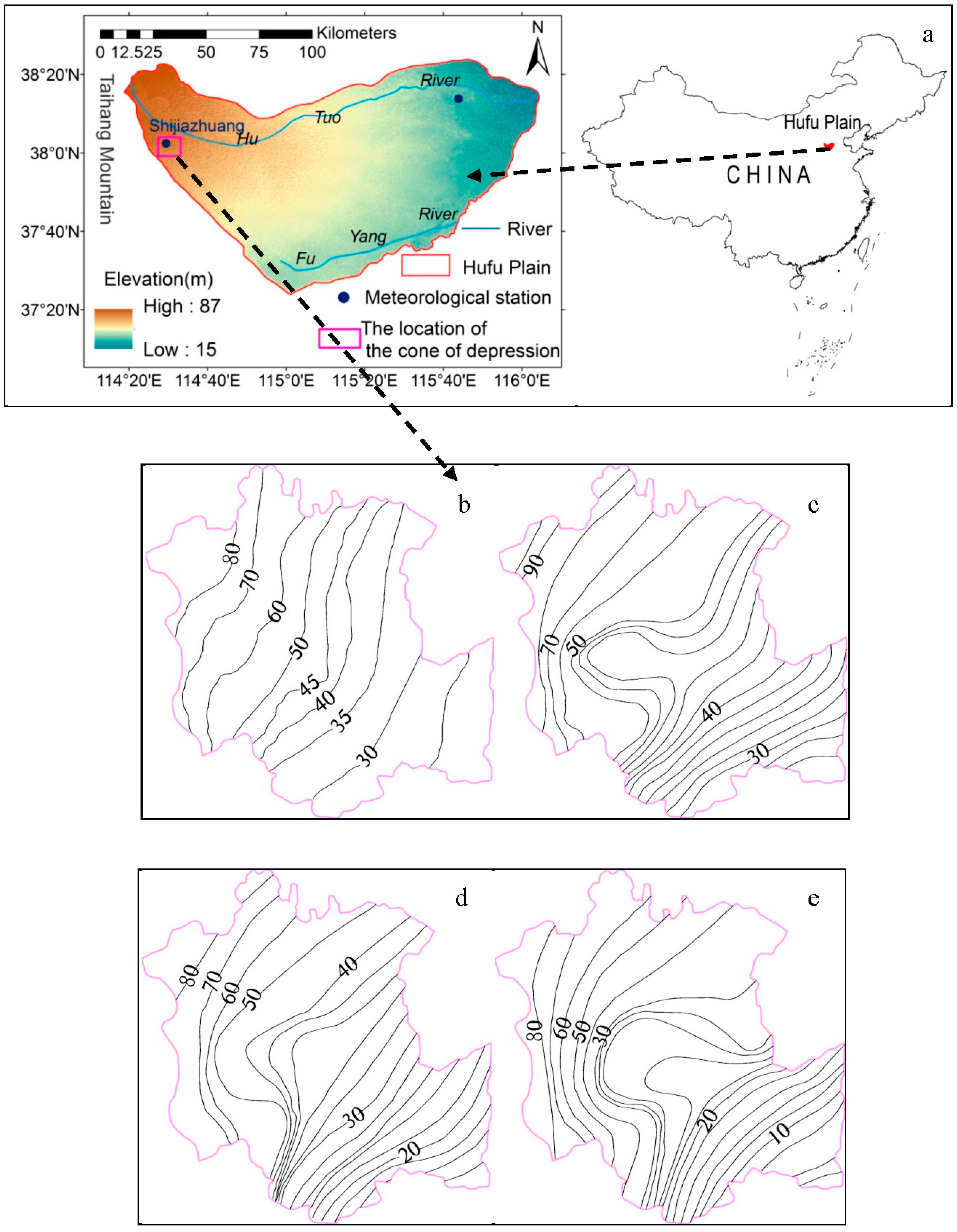
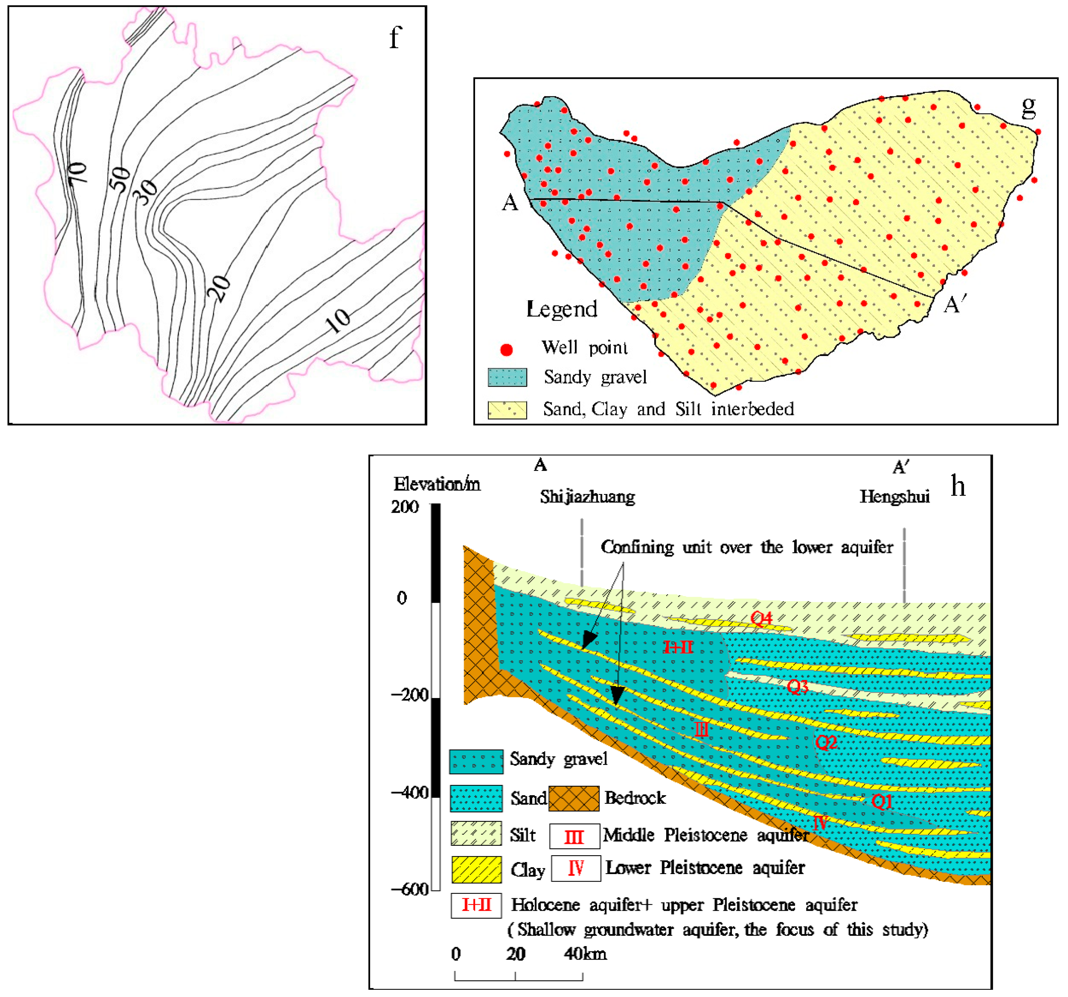
2.1. Study Areas

The Hufu Plain is located in the middle of the North China Plain (Figure 1a). It is bounded in the west by Mount Taihang and on the east, north, and south by gently undulating plains. The Hufu Plain has an area of about 8205 km2. The Hutuo River and Fuyang River are the main rivers in the Hufu Plain, and the annual runoff has decreased by over 80% [23] since the 1970s, because of the wholesale construction of the water storage projects upstream and the severe regional drought. The elevation of the Hufu Plain ranges from 15 to 87 m above sea level, and the annual precipitation ranges from 200 to 1000 mm/year, which is concentrated mostly in the summer.
The Hufu Plain aquifer can be divided into the following four zones [24]: the Holocene aquifer (I), the upper Pleistocene aquifer (II), the middle Pleistocene aquifer (III), and the lower Pleistocene aquifer (IV). Given the close connection between I and II, the two aquifer zones are hereafter described as the shallow groundwater aquifer (I + II). The three aquifer zones of I + II, III, and IV, as shown in Figure 1h, are separated by a relatively thick layer of clay, which acts as a confining unit over the lower zones.
The shallow groundwater aquifer (I + II) is unconfined, and the main geological deposit of this aquifer is sandy gravel with a depth of 20–40 m in the upper parts of the plain. In the middle parts of the plain, the aquifer is composed of alternate layers of sand, clay, sand, silt, and sand. The middle Pleistocene aquifer (III) and the lower Pleistocene aquifer (IV) are confined with a depth of over 20 m and consist of quaternary sediments of sandy gravel, sand, and clay, respectively.
The shallow groundwater aquifer is the main productive aquifer for the Hufu Plain, and is what this paper mainly deals with. Over 100 monitoring wells, mainly located in shallow groundwater aquifers, were selected (Figure 1g), which provided the groundwater level and drawdown records on monthly and yearly scales, and the depth of the wells varied from 9 m to 150 m [25,26].
Groundwater is an important water source for regional development and accounts for >80% of the total water supply, with irrigation as the main water use. Groundwater from the shallow, unconfined, aquifer layers is seriously overexploited, and the groundwater level declines by about 1 m each year [27,28]. In Shijiazhuang, the provincial capital of Hebei province, where the population is more than 17 million and the cropland accounts for over 50% of the total city region, the severe abstraction of the groundwater for living, industry, and irrigation has led to the formation of a constantly enlarging groundwater depression cone. The cumulative gross groundwater abstraction now has exceeded 18 billion m3 over the past 50 years in the groundwater depression cone [25].
According to the literature and site observations, there have been many climatic and environmental changes in the study area during the past few decades. For example, the annual precipitation significantly decreased in 1971–2010, compared with the 1950–1960s (Table 1). Since the 1970s, there has been a drastic decrease in the directly available surface water, and an increased demand for water in industrial and agricultural development due to the severe regional drought. The groundwater abstractions increased, leading to a consistent annual expansion in the area of the cone of depression of 8.63 km2/year, and a continued decline in the groundwater level in the center of the cone of depression, with a rate of 1.02 m/year [29]. Moreover, the water balance of the Hufu Plain has changed considerably over time. During 1961–1967, the total recharge was far larger than the discharge, and the surface water was an important water supply source; whereas during 1968–2010, with the construction of the large and medium-sized reservoirs in the upper reaches, and especially with the seepage treatment of the reservoir dam [30,31], the discharge volumes of the watercourse in the lower reaches and a lateral inflow from the mountain ranges in the west have reduced over 90% and 60%, respectively, and the recharge was less than the discharge [25].

2.2. Data

The data used in this study include meteorological data, input fluxes and output fluxes of the groundwater flow field, the groundwater level in the center of the cone of depression, and the area of the cone of depression (Figure 2); the average groundwater level of the Hufu Plain; and the groundwater level distribution area of the Hufu Plain over the period of 1961–2010. We used the groundwater level in the center of the cone of depression, the area of the cone of depression, and the average groundwater level of the Hufu Plain to characterize the groundwater flow field evolution as follows: (i) we used the groundwater level in the center of the cone of depression to implement the provided methodology of this study, (ii) the average groundwater level of the whole plain, the area of the cone of depression to test the rationality of the results of the step (i), if these two indexes evolution characterizes are obviously different in each division stages of a specific time scale, we consider the step (i) is suitable; if on the contrary, it is unsuitable.
The meteorological data in this study include the annual precipitation over 1961–2010. These data were obtained from a monthly precipitation dataset and a 0.5° × 0.5° resolution produced by the China Meteorological Administration (http://data.cma.cn), from two national meteorological stations (Figure 1a). The average groundwater level data of the Hufu Plain, the groundwater level in the center of the cone of depression, and the area of the cone of depression over 1961–1975 were provided by Liu [29], or can be obtained from the Yearbook of the Shijiazhuang Groundwater Level Statistical [26]. This resource determined the depression cone area based on whether the groundwater elevation contour normal direction changed, relative to the normal direction in the last year. The groundwater level distribution area data of the Hufu Plain were produced by Wang et al. [27], using an inverse distance weighted method through ArcGIS 10.0 (ESRI, Redlands, CA, USA). The curve of the ratio of groundwater recharge volume to exploitation volume (Re) over 1961–1975 was produced by Zhang et al. [23] using the groundwater numerical model.
The input fluxes (infiltration from precipitation, leakage of watercourses, infiltration from canal systems, infiltration from irrigation, and lateral influx from the mountain in the west) and output fluxes (exploitation, lateral out flux, and phreatic water evaporation, which was set as 0 according to Zhang [24]) of the groundwater flow field, the mean groundwater level of the Hufu Plain, the groundwater level in the center of the cone of depression and the area of the cone of depression from 1976 to 2010 were obtained from the Report on Geological Environmental Monitoring for Shijiazhuang [25], in which the input and output fluxes were estimated using the corresponding hydrogeology parameters and groundwater model. The curve of the ratio of the groundwater recharge volume to the exploitation volume (Re) over 1976–2010 was calculated using the data of the input and output fluxes, which fully considered the possible delay of the recharge. Digital elevation data with a resolution of 90 m were downloaded from the shuttle radar topography mission [32].

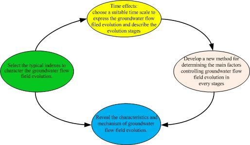
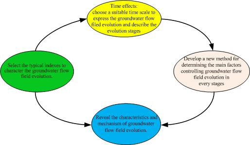
2.3. Research on Scale Effect

The DWT method was used to carry out the multi-scale time effect analysis for the identification of the characteristics of the groundwater system evolution. The DWT method is effective for multi-scale analysis. It can filter the research sequences at various time scales, eliminate high-frequency signals and noise, and then reconstruct the low-frequency signals obtained at a single scale [4]. Low frequency wavelet coefficients are reconstructed on various time scales into an identification quantity sequence to obtain an evolution trend and transition the time nodes of the research sequence at each time scale.
Firstly, Equation (1) is used to carry out DWT for the groundwater level in the center of the cone of depression, from 1961 to 2010, at the different time scales, and the low frequency wavelet coefficients and the high frequency wavelet coefficients are obtained for the different time scales, as follows:
w f ( a , b ) = | a | 1 2 Δ t k = 1 N ( f ( k Δ t ) ϕ ¯ ( k Δ t b a ) ) ,
where Wf(a, b) denotes the wavelet transform coefficient; φ(t) denotes the mother wavelet or basic wavelet function, according to the study by Sang et al. [33] and Wang et al. [4], ‘db3’ was chosen as the mother wavelet function in this study; φ ¯ ( t ) is the conjugate functions of the φ(t); a denotes expansion and contraction factor, reflecting the cycle length of wavelet; b denotes the time parameter, which is the shift factor relative to time, t; N signifies that the time, t, is divided into N equal parts, Δt = t/N; k denotes the time step; and f(t) is the groundwater level in the center of the cone of depression sequence over the period 1961–2010.
Secondly, Equation (2) was used to carry out single-scale reconstruction for each low-frequency signal of each scale, as follows:
f ( k Δ t ) = a , b w f ( a , b ) φ a , b ¯ ( k Δ t ) ,
Thirdly, based on the reconstruction low-frequency curve of the groundwater level in the center of the cone of depression in different time scales, the transition points of the groundwater system were identified, and the evolution trend of the curve between the two adjacent points was clarified using the method of linear regression analysis. Furthermore, in order to test the rationality of the transition point, an F test was used to compare the differences in the slope between the regression models. If p < 0.05, the transition points were considered to be significant. The SPSS11.5 software (IBM, New York, NY, USA) was used to carry out the regression analysis and F test.
Finally, the method of comparing and analyzing the evolution trend of the groundwater level in the center of the cone of depression at different time scales and the groundwater recharge–exploitation balance was used to determine the time nodes of the evolution stages of the groundwater flow fields in the research area. The ratio of groundwater recharge volume to exploitation volume (Re) can clearly explain the balance state of the groundwater system, where Re > 1 implies that the recharge of the groundwater system is larger than the discharge, while the groundwater system is in a state of increasing storage; Re < 1 indicates that the groundwater system is in a state of decreasing storage. The following five balance index categories can be distinguished: unbalanced toward to increasing storage state (Re ≥ 2.0), and the amount of the exploitation was less than one half of the recharge volumes; slightly unbalanced to increasing storage state (1 < Re < 2), and the amount of the exploitation was one half to 1.0 times that of the recharge volumes; balanced (Re = 1); slightly unbalanced toward to decreasing storage state (0.5 ≤ Re < 1), and the amount of the exploitation was one to two times that of the recharge volumes; and unbalanced toward to decreasing storage state (Re < 0.5), and the amount of the exploitation was more than 2.0 times that of the recharge volumes.

2.4. Dominant Factor Analysis

The following method was used to study the dominant factors at different evolutionary stages of the groundwater flow field. The dynamic model of groundwater system in the research area was defined as follows:
Q r r e + Q p r e + Q f r e + Q l r e + Q w r e Q l d i Q e v Q e x = Δ H μ F ,
where ΔH denotes the groundwater level amplitude, m; μ denotes the specific yield of the aquifer in the groundwater level amplitude zone, a dimensionless parameter; F denotes the area of the Hufu Plain, km2; Qrre denotes the input flux for the leakage of watercourse, m3; Qpre denotes the input flux of the precipitation infiltration, m3; Qfre denotes the input flux for the leakage of the canal irrigation field, m3; Qlre denotes the input flux of lateral influx, m3; Qwre denotes the input flux of well irrigation regression, m3; Qldi denotes lateral outfluxes, m3; Qex denotes the volume of groundwater exploitation, m3; and Qev denotes the volume of evaporation discharge of phreatic water, m3. The following equation is obtained by transforming Equation (3):
Δ H = 1 μ F ( Q r r e + Q p r e + Q f r e + Q l r e + Q w r e Q l d i Q e v Q e x ) ,
Through the analysis of Equation (4), it is clear that the input flux of the regional groundwater system increases the groundwater level, while the output flux decrease the groundwater level; the imbalance between input and output fluxes causes the ΔH change, which denotes the shift of the regional groundwater level; when the input flux is greater than the output flux, the groundwater level rises and ΔH > 0; when the groundwater level drops, ΔH < 0; and when the input flux is equal to the output flux, the groundwater level remains unchanged. When considering the distance of the movement of the groundwater level, in an evolution stage, the total distance of the movement of the groundwater level was calculated as follows:
D = 1 μ F ( Q r r e + Q p r e + Q f r e + Q l r e + Q w r e + Q l d i + Q e v + Q e x ) ,
Therefore, the effect of the intensity of each input flux and output flux of the groundwater system on the evolution of the groundwater flow field at a certain evolutionary stage was calculated using the following formula where the input flux is positive and the output flux is negative, as follows:
α i = ± Q i D μ F ,
where i denotes the serial number of input flux or output flux, Qi denotes the ith input or output flux, αi denotes the effect intensity of the ith input or output flux on groundwater flow field, and D is the distance of the groundwater level movement.
The fuzzy coincident matrix method [34] was used to calculate the dominant factors for the years with missing input and output flux data. Firstly, the main factors affecting the changes in the groundwater flow field were ordered based on what the groundwater scientist qualitatively decides is important, according to their experience. Then, according to the order of ‘importance’, a binary comparison between every two pairs was carried out separately, based on the experiences of the scientist. For example, a binary comparison was made between the ‘importance’ of groundwater exploitation quantity (ai) and that of the precipitation infiltration (aj). If ai is more important than aj, rij = (0.6–1.0), rji = (0–0.5), and rij + rji = 1.0. If ai and aj are equally important, rij = 0.5, rji = 0.5; if aj is more important than ai, rji = (0.6–1.0), rij = (0–0.5), and rij + rji = 1.0 (i = 1, 2, …, n; j = 1, 2, …, n). Correspondingly, a priority matrix (R = [rij] n × n) of each evolution stage was obtained. The uniform transformation (Equations [7] and [8]) was carried out for the priority matrix to obtain the fuzzy coincident matrix (B = [bi] n × 1), and square root normalization (Equation (9)) was carried out for the fuzzy coincident matrix, generating the weight matrix (W = (ωi) n × 1), as follows:
b i j = b i b j 2 n + 0.5 ,
B i = j n b i j n ,
w i = B i i n B i ,

2.5. Quantitative Analysis

A regression analysis was used to evaluate the quantitative relationships between the groundwater flow field evolution, precipitation changes, and groundwater exploitation. A regression analysis on the groundwater level series, precipitation series, and groundwater exploitation volume series were performed to establish the regression equations, and a t-test was used to test the significance of the regression models. The statistical software SPSS11.5 was used to conduct these analyses.

3. Results

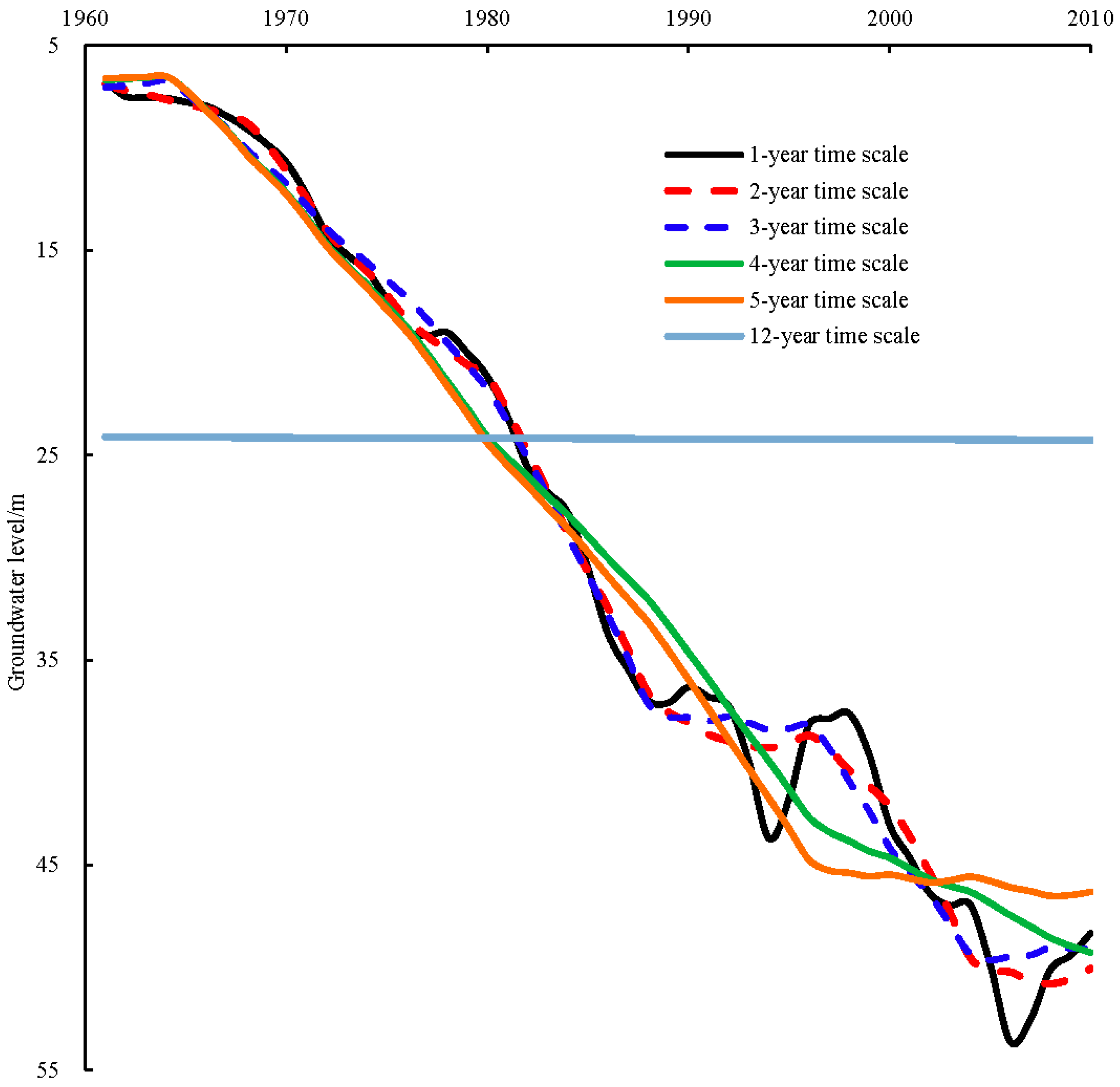
3.1. Scale Effect and Stage Division of the Evolution of the Groundwater Flow Field

Using the groundwater level in the center of the cone of depression at different time scales of the Hufu Plain combined with the F test, the balance index (Re) categories of the groundwater system to demonstrate how a particular choice of the suitable time step and the division of the evolution stage was made. Firstly, the methods described in Section 2.3 were used to obtain the 1–5-year and 12-year (Figure 3) time scale maps of the evolution characteristics of the groundwater flow field in the research area. As shown in Figure 3, there was a significant difference in the groundwater level among the six time scales, because the high-frequency signals and noise of the original time series were eliminated gradually with the time scales’ increase, retaining only the interesting part of the original signal, depending on the application. We can therefore use these data to investigate the scale-dependent variations of the groundwater level signals that contain transient features, allowing us to identify different important stages of evolution within a time scale series, and to study these stages individually. Based on Figure 3, we can roughly estimate the transition points of the groundwater system evolution in each time scale.
Secondly, we used the F test to compare the evolution slope differences between the linear regression model for each division in each time scale, eliminated the transition points that are statistically not significant, and then got the exact time nodes of the groundwater system evolution of different time scales. There were five transition points on the two-year time scale (1968, 1980, 1988, 1995, and 2005; Figure 3a), dividing the whole sequence into six divisions. There were seven transition points in the evolution of the groundwater flow field at the one-year time scale (1967, 1976, 1988, 1991, 1994, 1998, and 2006; Figure 3b), dividing the whole sequence into eight divisions. There were five transition points on the three-year time scale (1964, 1980, 1988, 1995, and 2005; Figure 3c), dividing the whole sequence into six divisions. There were two transition points in the four-year and five-year time scale (1964 and 1995; Figure 3d,e), dividing the whole sequence into three divisions. There were no transition points on the 12-year time scale (Figure 3f).
Thirdly, use of the balance index (Re) categories of the groundwater system to test the rationality of the stages divisions of the groundwater system evolution of different time scales, if the balance state (balance index (Re) categories) of the groundwater system in the different division stages of a specific time scale is obviously different, we consider this time scale as suitable; if on the contrary, it is unsuitable. There were five transition points on the two-year time scale (Figure 3a), dividing the evolution of the groundwater flow field into the following six stages: 1961–1967, 1968–1980, 1981–1988, 1989–1995, 1996–2005, and 2006–2010. Compared with the curve, Re, during 1961–1967, Re was greater than 2.0, the flow field was in a state of unbalanced toward to increasing storage, and the groundwater level remained basically unchanged. During 1968–1980, Re was in 1.0–2.0 (except for 1973 and 1976), on average, Re = 1.32, the groundwater flow field was in a state of slightly unbalanced toward increasing storage. During 1981–1995, the average value of Re was 0.46, which implies the groundwater system was generally in a state of unbalance toward to the decreasing storage. In 1988, the Re = 0.38, and several years before and after the nodes it was less than 0.5, so the time nodes of 1988 should be eliminated. During 1996–2004, Re increased during the catastrophic flood period (1996 when the precipitation was 1096 mm), but it was still less than 1.0 in the other years, on average, Re = 0.70, the flow field was in a state of slightly unbalanced towards the decreasing storage, and the groundwater level continued to decline. From 2006–2010, Re = 0.40, the groundwater flow field was in a state of unbalance towards the decreasing storage. Overall, the transition points on a two-year time scale can clearly express the evolution stages of the groundwater flow field.
Figure 3b shows that the time nodes of a one-year time scale did not coincide with curve Re, especially the nodes of 1991 and 1994. The Re of several years before and after the nodes was less than 0.5. During this period, the groundwater flow field was generally in a state of unbalance toward the decreasing storage, and it could not be divided into an evolution stage. On the four-year time scale and five-year time scale, there were no transition points during 1965–1997. Considering the evolutionary sequence of the groundwater recharge–exploitation balance (Re), Re rapidly changed from >1.0 to <1.0 during 1965–1997. The groundwater flow field changed from a state of increasing storage to a state of decreasing storage. However, these stages and their characteristics were eliminated. On the 12-year scale (Figure 3f), the evolution characteristics of the groundwater flow field formed a straight line with all of the evolution characteristics being generalized, and all of the features of each stage lost. The groundwater flow field evolution shows no stage characteristics on a large scale such as this.
Compared with the two-year time scale, the one-year time scale reflects more transition points during groundwater flow field evolution, and the stage divisions are not sufficiently clear. At the three-year time scale, the first transition point, 1964, is not accurate, because the Re was generally greater than 2.0 during 1961–1967, and the groundwater flow field was in a state of unbalance toward increasing storage. At the 4-, 5-, and 12-year time scales, the characteristics of the stages were lost. Some transition points during the evolution process were over-homogenized and obscured. Therefore, we adopted the two-year time scale to divide groundwater flow field evolution into five stages. During 1961–1967, the groundwater was in a natural state, so the field was a natural flow field. During 1968–1980, the annual average exploitation volumes were 2.13 billion m3/year, but due to several drought years (e.g., the precipitation was 224 and 304 mm in 1973 and 1975, respectively), the groundwater system was subject to mild overexploitation. During 1981–1995, the annual average exploitation volume was 2.56 billion m3/year, and the accumulated overexploitation volume was 9.4 billion m3 [25], forming a stable groundwater depression cone. During 1996–2005, the exploitation volumes were 2.29 billion m3/year, the overexploitation volumes increased to 15.4 billion m3 [25], which was serious overexploitation. During 2006–2010, the exploitation volume was 1.98 billion m3/year [25], making the period an exploitation reduction stage.
In the process of the choice of the time-step and the division of the different stages, we used the F test to reduce the subjectivity of the selection of the transition points, using the transition of the state of the groundwater flow field to test the rationality of the division of the evolution stages; however, a few transition points may need to be eliminated in accordance to the state of the groundwater system, which may still rely on the experience of the groundwater scientist, so the experience of the scientist should always be valued.

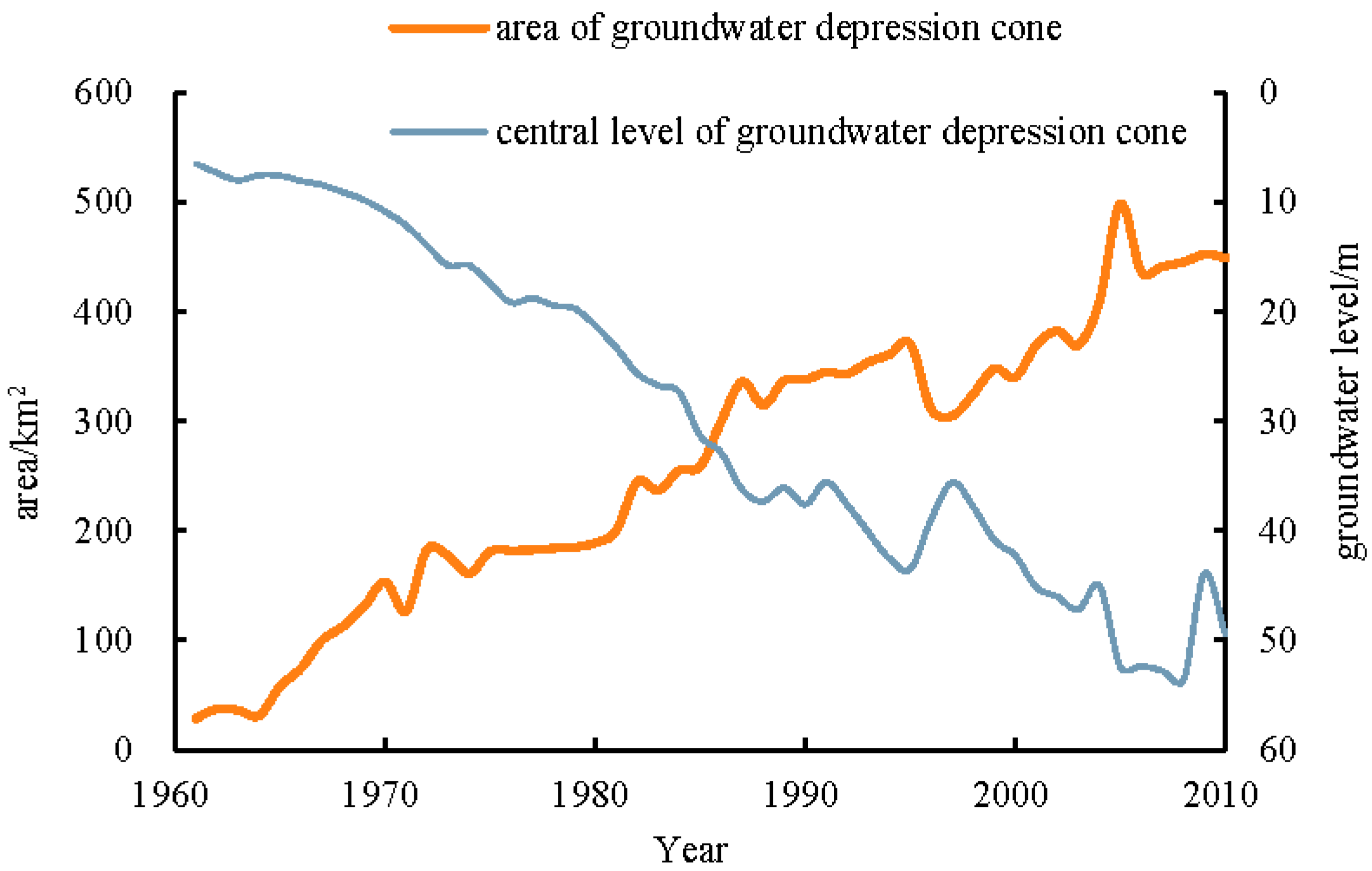
3.2. Characteristics of Groundwater Flow Field Evolution

The Figure 1b–f shows the groundwater elevation in the area of the cone of depression for the natural flow field, mild overexploitation, depression cone formation, and exploitation reduction stage. In the natural flow field stage (1961–1967), the groundwater level in the research area was characterized by a change from a deep to shallow groundwater level in the area from the West Piedmont to the Eastern Plain. The groundwater level in this area was less than 10 m and the distribution areas mainly had groundwater levels of <5 m (Table 2). No obvious groundwater depression cone was formed.
In the mild overexploitation stage (1968–1980), the area with groundwater levels of <5 m was significantly reduced. The distribution areas mainly have groundwater levels of 5–10 m. The distribution areas with groundwater levels >10 m appear, with an area reaching 1889 km2, accounting for 23.1% of the total regional area. The analysis of the linear regression (p < 0.05) showed that the rate of decline of the groundwater level was 0.38 m/year, the groundwater level in the center of the cone of depression descended at a speed of 1.01 m/year, while the area of the cone of depression expanded at 6.37 km2/year.
In the depression cone formation stage (1981–1995), the ratio of the distribution area with groundwater level of less than 10 m to the Hufu Plain shrank drastically. Distribution areas mainly have a groundwater level of 10–25 m, and the areas with groundwater levels of more than 35 m appear, accounting for 4.2% the area of the total region. The rate of decline of the average groundwater level in the region was 0.69 m/year. The average annual rate of descent in the groundwater level in the center of the cone of depression was 1.35 m/year, and the area of the cone of depression was increased by 11.35 km2/year.
In the serious overexploitation stage (1996–2005), the distribution area, with groundwater levels of <20 m, shrank drastically and mainly had groundwater levels of 30–40 m. The distribution areas with groundwater levels of >45 m occurred, accounting for 4.7% of the total area. The rate of descent of the average groundwater level in the region was 0.69 m/year. The average rate of descent of the groundwater level in the region was increased by 0.34 m/year, compared with the rate in the depression cone formation stage, and the spread rate of the area of the cone of depression was accelerated to 12.39 km2/year.
In the exploitation reduction stage (2006–2010), the exploitation volume in the serious overexploitation area decreased each year. The rate of descent of the regional average groundwater level was 0.74 m/year. The expansion of the area of the cone of depression slowed during this stage.

3.3. Analysis of Dominant Factors

During 1961–1967, the groundwater flow field showed natural stage characteristics. The fuzzy coincident matrix method was used to calculate the magnitude of the main controlling factors, because of a lack of input and output flux data. The ranking of the relative importance of each input and output flux was as follows: infiltration from precipitation > exploitation > leakage of watercourse > infiltration from irrigation > infiltration from canal system > lateral influx > lateral outflux. A binary comparison was made between each two, according to the order of exploitation, infiltration from precipitation, leakage of watercourse, infiltration from canal system, infiltration from irrigation, lateral influx, and lateral outflux, and a priority matrix was obtained (Equation (10)). The following weight matrix was obtained by uniform transformation (Equations (7) and (8)) and square root normalization (Equation (9)) of the priority matrix, as follows: (0.20, 0.23, 0.15, 0.11, 0.12, 0.10, and 0.08).
[ 0.50 0.30 0.70 0.80 0.80 0.90 0.90 0.70 0.50 0.80 0.90 0.90 0.90 1.00 0.30 0.20 0.50 0.60 0.60 0.70 0.70 0.20 0.10 0.40 0.50 0.40 0.50 0.60 0.20 0.10 0.40 0.60 0.50 0.60 0.60 0.10 0.10 0.30 0.50 0.40 0.50 0.50 0.10 0.00 0.30 0.40 0.40 0.40 0.50 ]
For the mild overexploitation, depression cone formation, serious overexploitation, and exploitation reduction stages, Equations (3)–(6) were used for calculation. The results are shown in Table 3. Infiltration from precipitation had the largest effect in the natural flow field stage and was the main controlling factor, followed by exploitation. In the mild overexploitation, depression cone formation, serious overexploitation, and exploitation reduction stages, exploitation had the largest effect and was the main controlling factor, followed by infiltration from precipitation.

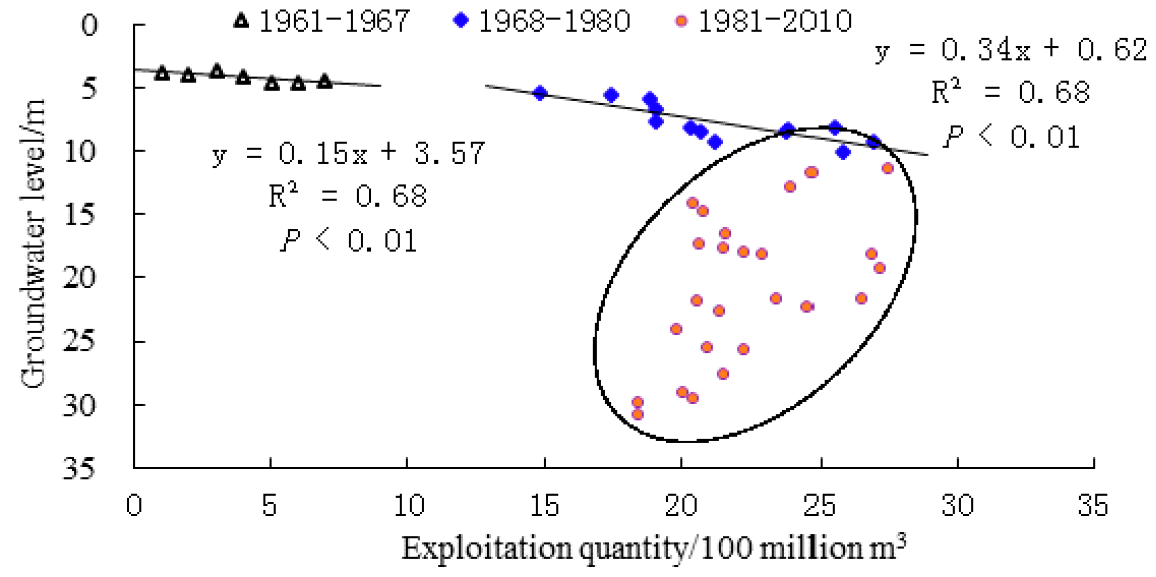
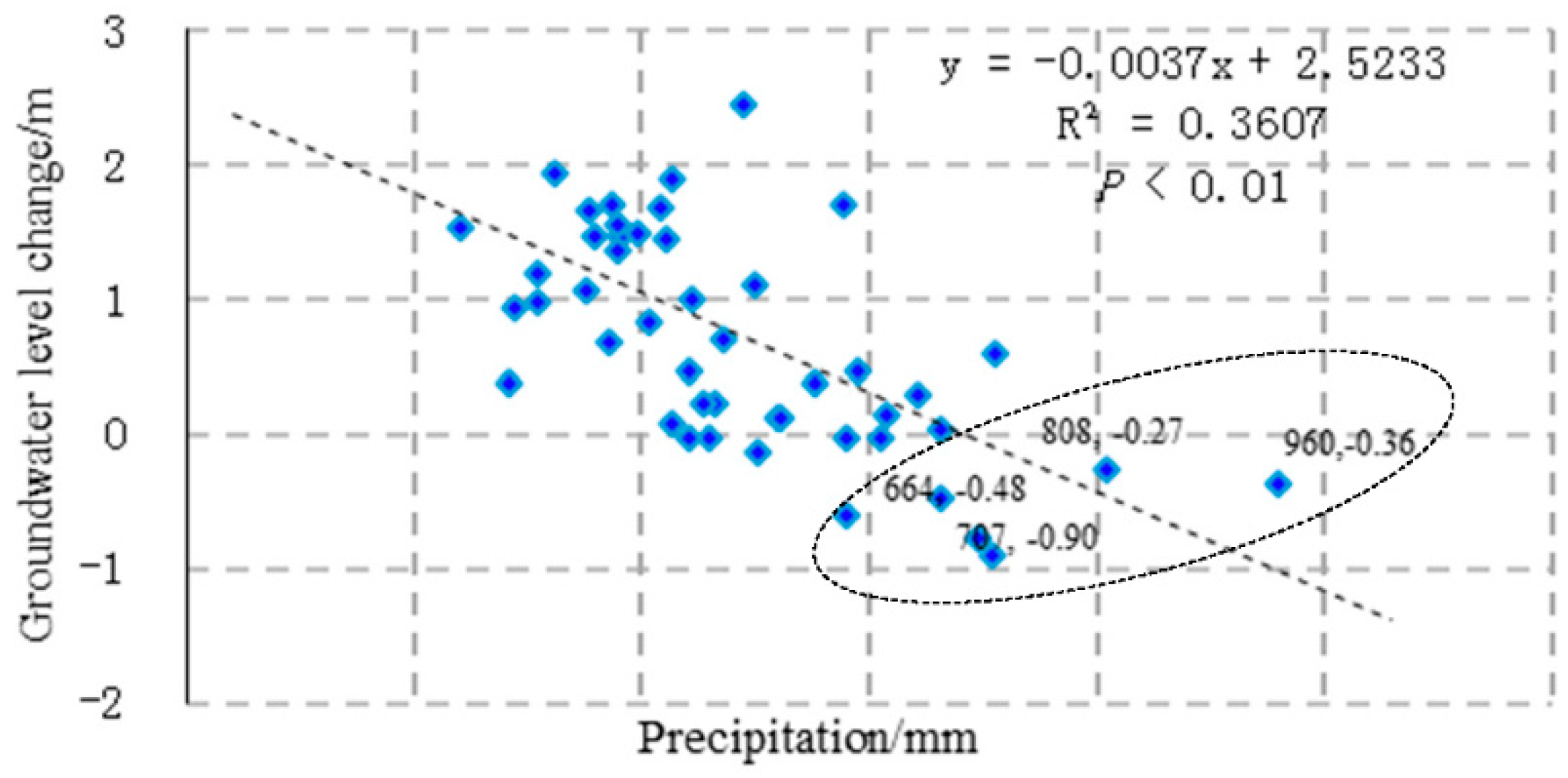
3.4. Quantitative Analysis of Influence of Precipitation and Exploitation on Groundwater Levels

Exploitation was the main factor causing the decline of the groundwater level, and precipitation is an important factor influencing the changes in the groundwater level. In the natural flow field and the mild overexploitation stages, of only a few years in duration, the groundwater system was in a state of decreasing storage, and the groundwater levels responded sensitively to the changes in the exploitation quantity. In the natural flow field and mild overexploitation stages, there was a clear correlation between the exploitation quantity and the groundwater level. A regression analysis suggested that when the exploitation volumes were increased by 100 million m3, the mean groundwater level in the research areas decreased by 0.15 m in the natural flow field stage, and decreased by 0.34 m in the mild overexploitation stage (Figure 4).
During the depression cone formation, serious overexploitation, and exploitation reduction stages, the volumes of the groundwater abstraction were far greater than the recharge volume. In Figure 4, the data from 1981–2010 are shown as scattered dots, and the relationship between the groundwater level and exploitation volumes is not obvious. Moreover, according to Equation (4), under the condition of the total output fluxes being larger than the input fluxes, even if the exploitation declined, the groundwater level would continue to descend. However, the increased precipitation can slow the decline of the groundwater level. Figure 5 shows that when the precipitation amount was increased by 100 mm, the descent amplitude of the groundwater level dropped by 0.37 m. In some years, with ample precipitation, the groundwater level even rose. For example, the precipitation was 1096 mm in 1995–1996. During this period, the groundwater exploitation reduced, the recharge increased, the total input fluxes were larger than output fluxes, and the groundwater levels correspondingly rose.

4. Discussion

In this paper, we use the groundwater level in the center of the cone of depression at different time scales of the Hufu Plain, combined with the F test and the balance index (Re) categories of the groundwater system, so as to study the shallow groundwater aquifer system evolution time scale effects and mechanisms, and the applicability of the method to other types of aquifers needs to be tested in future studies.
The DWT method was used to carry out the multi-scale time effects analysis for the groundwater level in the center of the cone of depression from 1961 to 2010, and get the 1–5-year and 12-year time scale maps of the evolution characteristics of the groundwater flow field in the research area (Figure 3, Figure 6); based on the maps, we can roughly estimate the transition points of the groundwater system evolution in each time scale. Compared with the original groundwater level time series (Figure 2), the one-year time scale time series is similar to the original series, and with the time scale increasing, more and more details of the time series were filtered; as the time scale increased to 12 years, the evolution of the groundwater level formed a straight line and all of the evolution characters were generalized, so it is necessary for us to identify a suitable time scale for more clearly expressing the groundwater system evolution. Although our methodology can be used in any regions where groundwater is the main water supply, the time scale effects may be significantly different for various study areas, because of the difference of the hydrogeology conditions. In the same time scale, the characters of the groundwater system evolution for the different study areas may be different, and the time series evolution characters as the time scales increase are also varied, so you probably choose different time scales to study the groundwater evolution for the different regions.
In order to reduce the subjectivity of the choice of the suitable time step and the division of the different evolution stages, we quantified the balance index (Re) of the groundwater system. The following five balance index categories can be distinguished: unbalanced toward to increasing storage state (Re ≥ 2.0); slightly unbalanced to increasing storage state (1 < Re < 2); balanced (Re = 1); slightly unbalanced toward to decreasing storage state (0.5 ≤ Re < 1); and unbalanced toward to decreasing storage state (Re < 0.5), which can help us discriminate the stage of the divisions of the groundwater system evolution of the different time scales, but in the process of the division of the evolution stages, the experiences of the groundwater scientists are required, and thus the researchers who are not specialists in groundwater science may meet some difficulties when utilizing the methods.

5. Conclusions

The paper provides a new method to study the groundwater flow field temporal evolution characteristics, focusing on the choice of the correct time step for identifying the distinct stages of evolution characterized by different characteristics linked to the management of groundwater system. The Hufu Plain was taken as a case study to demonstrate the methodology. The results showed that a two-year time scale was the most suitable for studying the groundwater flow field evolution in the Hufu Plain. According to the groundwater level on two-year time scale, we can divide the groundwater flow field evolution into the following five stages: natural flow field, mild overexploitation, depression cone formation, serious overexploitation, and exploitation reduction.
The main factors controlling the groundwater evolution were then assessed for the different stages, still using the transformed two-year time scale groundwater level time series. The infiltration from precipitation was the main factor controlling groundwater level changes during the natural flow field and the effect intensity was 23%. During the mild overexploitation, depression cone formation, serious overexploitation, and exploitation reduction stages, the effect of the intensity of the exploitation was 43.5%, 52.25%, 55.96%, and 53.47%, respectively, and it was the main controlling factor. With the methodology, after careful tests on a number of different systems, we can obtain an increased knowledge regarding regional groundwater dynamics.

Author Contributions

D.W., G.Z., H.F. and J.W. conceived, designed, and conducted the research, but also collected and analyzed the data. Y.T. reviewed and edited the paper; He was also the corresponding author.

Funding

This research was funded by the National Natural Science Foundation of China (NSFC) (Project No. 41172214, 41502253, 41702263, 51822907, 51479210); Research and demonstration of water quality guarantee and ecological restoration technology in the World Horticultural Exposition and winter Olympics in Gui river basin (2017ZX07101004).

Acknowledgments

We thank LetPub (www.letpub.com) for its linguistic assistance during the preparation of this manuscript.

Conflicts of Interest

The authors declare no conflict of interest.

References

  1. Murphy, J.M.; Sexton, D.M.H.; Jenkins, G.J. UK Climate Projections Science Report: Climate Change Projections; Met Office Hadley Centre: Exeter, UK, 2009. [Google Scholar]
  2. Xu, Y.Q.; Mo, X.G.; Cai, Y.L.; Li, X.B. Analysis on groundwater table drawdown by land use and the quest for sustainable water use in the Hebei Plain in China. Agric. Water Manag. 2005, 75, 38–53. [Google Scholar] [CrossRef]
  3. Perrina, J.; Ferrant, S.; Massuel, S.; Dewandel, B.; Maréchal, C.; Aulong, S.; Ahmed, S. Assessing water availability in a semi-arid watershed of southern India using a semi-distributed model. J. Hydrol. 2012, 460–461, 143–145. [Google Scholar] [CrossRef]
  4. Wang, W.S.; Ding, J.; Li, Y.Q. Hydrogeology Wavelet Analysis; Chemical Industry Press: Beijing, China, 2005. [Google Scholar]
  5. Nalley, D.; Adamowski, J.; Khalil, B. Using discrete wavelet transforms to analyze trends in stream flow and precipitation in Quebec and Ontario (1954–2008). J. Hydrol. 2012, 475, 204–228. [Google Scholar] [CrossRef]
  6. Parkin, G.; Birkinshaw, S.J.; Younger, P.L.; Rao, Z.; Kirk, S. A numerical modeling and neural network approach to estimate the impact of groundwater abstractions on river flows. J. Hydrol. 2007, 339, 15–28. [Google Scholar] [CrossRef]
  7. Padilla, F.; Méndez, A.; Fernández, R.; Vellando, P.R. Numerical modeling of surface water/groundwater flows for freshwater/saltwater hydrology: The case of the alluvial coastal aquifer of the Low Guadalhorce River, Malaga, Spain. Environ. Geol. 2008, 55, 215–226. [Google Scholar] [CrossRef]
  8. Yidana, S.M.; Alfa, B.; Banoeng-Yakubo, B.; Addai, M.O. Simulation of groundwater flow in a crystalline rock aquifer system in Southern Ghana—An evaluation of the effects of increased groundwater abstraction on the aquifers using a transient groundwater flow model. Hydrol. Process. 2012, 28, 1084–1094. [Google Scholar] [CrossRef]
  9. Iwasaki, Y.; Nakamura, K.; Horino, H.; Kawashima, S. Assessment of factors influencing groundwater—Level change using groundwater flow simulation, considering vertical infiltration from rice—Planted and crop-rotated paddy fields in Japan. Hydrogeol. J. 2014, 22, 1184–1855. [Google Scholar] [CrossRef] [Green Version]
  10. Lafare, A.E.A.; Peach, D.E.; Hughes, A.G. Use of seasonal trend decomposition to understand groundwater behavior in the Permo—Triassic Sandstone aquifer, Eden Valley, UK. Hydrogeol. J. 2016, 24, 141–158. [Google Scholar] [CrossRef]
  11. Asmuth, J.R.; Maas, K.; Bakker, M.; Petersen, J. Modeling Time Series of Groundwater Head Fluctuations Subjected to Multiple Stresses. Groundwater 2008, 46, 30–40. [Google Scholar] [CrossRef]
  12. Bloomfield, J.P.; Marchant, B.P. Analysis of groundwater drought building on the standardized precipitation index approach. Hydrol. Earth Syst. Sci. 2013, 17, 4769–4787. [Google Scholar] [CrossRef] [Green Version]
  13. Chae, G.T.; Yun, S.T.; Kim, D.S.; Kim, K.H.; Joo, Y. Time—Series analysis of three years of groundwater level data (Seoul, South Korea) to characterize urban groundwater recharge. Q. J. Eng. Geol. Hydrogeol. 2010, 43, 117–127. [Google Scholar] [CrossRef]
  14. Wang, W.S.; Yuan, P.; Ding, J. Wavelet analysis and its application to stochastic simulation of daily flow. J. Hydraul. Eng. 2000, 11, 43–48. (In Chinese) [Google Scholar]
  15. Kang, L.; Liu, S.R.; Liu, X.Z. Multiresolution and periodicity analysis of hydrological and meteorological factors in upper reaches of Minjiang River. Acta Ecol. Sin. 2016, 36, 1253–1262. (In Chinese) [Google Scholar]
  16. Zhang, G.H.; Fei, Y.H.; Zhang, X.N.; Yan, M.J. Abnormal variation of groundwater flow field in plain area of Hutuo River basin and analysis on its cause. J. Hydraul. Eng. 2008, 39, 747–752. (In Chinese) [Google Scholar]
  17. Yang, Y.H.; Watanabe, M.; Sakura, Y.; Tang, C.Y.; Hayashi, S. Groundwater table and recharge changes in the Piedmont region of Taihang Mountain in Gaocheng City and its relation to agricultural water use. Water SA 2002, 28, 171–178. [Google Scholar] [CrossRef]
  18. Kendy, E.; Zhang, Y.Q.; Liu, C.M.; Wang, J.X.; Steenhuis, T. Groundwater recharge from irrigated cropland in the North China Plain: Case study of Luancheng County, Hebei Province, 1949–2000. Hydrol. Process. 2004, 18, 2289–2302. [Google Scholar] [CrossRef]
  19. Shu, Y.Q.; Villholth, K.G.; Jensen, K.H.; Stisen, S.; Lei, Y. Integrated hydrological modeling of the North China Plain: Options for sustainable groundwater use in the alluvial plain of Mt. Taihang. J. Hydrol. 2012, 464–465, 79–93. [Google Scholar] [CrossRef]
  20. Du, S.H.; Su, X.S.; Lu, H. The Artificial Recharge Effects of Groundwater Reservoir under Different Precipitation Plentiful Scanty Encounter in Hutuo River. J. Jilin Univ. (Earth Sci. Ed.) 2010, 40, 1090–1097. (In Chinese) [Google Scholar]
  21. Nakayama, T.; Yang, Y.H.; Watanabe, M.; Zhang, X.Y. Simulation of groundwater dynamics in the North China Plain by coupled hydrology and agricultural models. Hydrol. Process. 2006, 20, 3441–3466. [Google Scholar] [CrossRef] [Green Version]
  22. Hu, Y.K.; Moiwo, J.P.; Yang, Y.H.; Han, S.M.; Yang, Y.M. Agricultural water saving and sustainable groundwater management in Shijiazhuang Irrigation District, North China Plain. J. Hydrol. 2010, 393, 219–232. [Google Scholar] [CrossRef]
  23. Zhang, G.H.; Fei, Y.H.; Nie, Z.L.; Yan, M.J. Theory and Method of Regional Groundwater Flow Field Evolution and Assessment; Sciences Press: Beijing, China, 2014. [Google Scholar]
  24. Zhang, Z.J. Investigation and Assessment of Sustainable Utilization of Groundwater Resources in North China Plain; Geological Publishing House: Beijing, China, 2009; pp. 157–180. ISBN 978-7-116-06105-7. [Google Scholar]
  25. Geological Environmental Monitoring Institute of Hebei Province (GEMIHP). Report on Geological Environmental Monitoring of Shijiazhuang of 1981–1985, 1986–1990, 1991–1995, 1996–2000, 2001–2005, 2006–2010. Available online: www.ngac.cn/125cms/c/qggnew/index.htm (accessed on 17 August 2018).
  26. GEMIHP. Yearbook of Shijiazhuang Groundwater Level Statistical of 1961–1980. Available online: www.ngac.cn/125cms/c/qggnew/index.htm (accessed on 17 August 2018).
  27. Wang, J.Z.; Zhang, G.H.; Yan, M.J.; Nie, Z.L. Research on the Plot Groundwater spatial-temporal Evolvement Rule in Hutuo Valley. J. Arid Land Resour. Environ. 2009, 23, 5–11. (In Chinese) [Google Scholar]
  28. Mao, X.S.; Liu, C.M. Groundwater changing trends and agriculture sustainable development in Taihang mountain foot Plain of North China. Res. Soil Water Conserv. 2001, 8, 147–149. (In Chinese) [Google Scholar]
  29. Liu, Z.P. Impact of Agricultural Activities on Regional Groundwater Variation—A Case of Shijiazhuang Plain. Ph.D. Thesis, Chinese Academy of Geological Sciences, Beijing, China, 2007. [Google Scholar]
  30. Fei, Y.H. The influence of Huangbizhuang reservoir dam foundation seepage cut-off on the downstream development and counter measures. Site Investig. Sci. Technol. 1996, 6, 13–15. (In Chinese) [Google Scholar]
  31. He, P. Primary Analysis of Groundwater Circumstances Influence of Huangbizhuang Village Reservoir Water proof Project to the Hutuo River Alluvium. Ground Water 2009, 31, 121–123. (In Chinese) [Google Scholar]
  32. Jarvis, A.; Reuter, H.I.; Nelson, A.; Guevara, E. Hole-Filled Seamless SRTM DataV4. International Center for Tropical Agriculture. Available online: http://srtm.csi.cgiar.org (accessed on 17 August 2018).
  33. Sang, Y.F.; Wang, D. Wavelet selection method in hydrologic series wavelet analysis. J. Hydraul. Eng. 2008, 39, 295–300. (In Chinese) [Google Scholar]
  34. Zhang, J.; Zhang, L.C.; Xu, C.M.; Zhang, J.Z.; Li, X.B. Application of fuzzy consistent matrix method in multi-objective decision plain of slim hole drilling. Nat. Gas Ind. 2003, 23, 61–62. (In Chinese) [Google Scholar]
Figure 1. (a) The Hufu Plain research area, the groundwater level depression cone area; (b) groundwater elevation in the area of the cone of depression for 1961, (c) 1980, (d) 1995, (e) 2005, and (f) 2010; (g) lithological and monitoring wells distribution of the shallow groundwater aquifer; and (h) hydrostratigraphy along the cross-section line marked AA′ in (g).
Sustainability 10 02972 g001aSustainability 10 02972 g001b
Figure 2. Variation of the original groundwater level in the center of the cone of depression and the area of the cone of depression from 1961–2010.
Sustainability 10 02972 g002
Figure 3. Evolution characteristics of the groundwater flow field in the research area using (a) a two-year time scale, (b) a one-year time scale, (c) a three-year time scale, (d) a four-year time scale, (e) a five-year time scale, (f) a twelve-year time scale. (g) The curve of the ratio of groundwater recharge volume to exploitation volume, the symbol Sustainability 10 02972 i001 
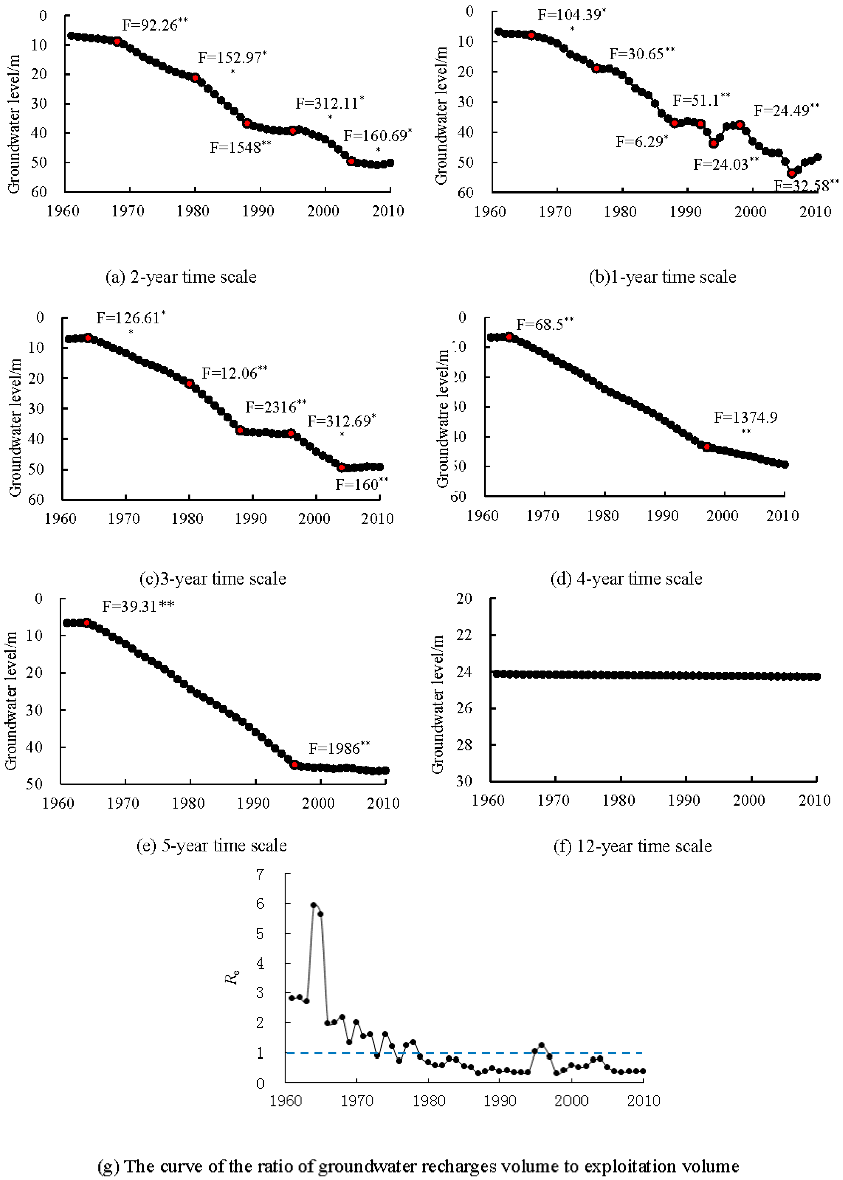
indicates the transition points, and the labels provide the F test values between the division sequences linear regression model slope, * indicates significance levels of 0.05, ** indicates significance levels of 0.01.
Sustainability 10 02972 g003
Figure 4. Relationship between exploitation quantity and groundwater level.
Sustainability 10 02972 g004
Figure 5. Relationship between precipitation and change in groundwater level.
Sustainability 10 02972 g005
Figure 6. The groundwater level evolution characteristics with the time scale increasing.
Sustainability 10 02972 g006
Table 1. The variation characteristics of average precipitation in different decades.
DecadesPrecipitation/mmRange of Variation/%
1951–1960614.20.00
1961–1970525.514.4
1971–1980467.0−24.0
1981–1990477.5−22.3
1991–2000470.4−23.4
2001–2010472.0−23.2
Notes: the annual precipitation range of variation in 1961–1970, 1971–1980, 1981–1990, 1991–2000, and 2011–2010 were calculated relative to the annual precipitation in 1951–1960.
Table 2. The groundwater level distribution area of the Hufu Plain in each evolution stage (km2).
Year<5 m5–10 m10–15 m15–20 m20–25 m25–30 m30–35 m35–40 m40–45 m>45 m
19657945260
19757915525183257
198523919323788190425289
1995622932011120928511386315762
20051825775812778939082024174229630
Table 3. Intensity levels of each input flux and output flux of the groundwater flow field (unit: %).
Equilibrium ElementsEvolution Stage
Natural Flow Field StageMild Overexploitation StageDepression Cone Formation StageSerious Overexploitation StageExploitation Reduction Stage
Input fluxesInfiltration from precipitation23.0019.1920.6720.0624.30
Leakage of watercourse15.002.823.124.680.81
Infiltration from canal system11.009.483.242.401.82
Infiltration from irrigation12.0011.398.127.727.71
Lateral influx10.008.288.776.735.88
Subtotal71.0051.1543.9241.5840.52
Output fluxesExploitation20.0043.4552.2455.9653.47
Lateral outflux8.005.393.842.476.01
Subtotal28.0048.8556.0858.4359.48

