1. Introduction
The interest in hybrid and electric vehicles has constantly been growing due to the rising ecological sensitivity driven by government regulations [
1,
2]. Fully electric vehicles (FEVs) have been of interest in academia and industry as they provide a local carbon-free mobility solution. The development of new layout concepts for electric vehicles has been improved significantly, associated with the significant advances in energy storage units and the motor’s power density evolution. The first electric vehicle concept was to replace the internal combustion engine with one electric motor, keeping the same transmission structure, with a single centrally located drive system and a single transmission speed. Gradually, this architecture has been replaced by individually controlled electrical systems to increase driving safety and performance. New vehicle architectures comprising one, two, three, or four independently controlled electric motors have shown different advantages [
3,
4,
5,
6]. In addition to optimizing the internal design, providing more space to accommodate energy storage units, and eliminating elements like drive shafts, gearboxes, and differential, independent electric motors can drastically change vehicle performance. The advantage of using the four individual motors configuration is that it allows for precise torque distribution when applying the maximum motor power [
7,
8,
9,
10,
11]. This solution allows individual control of the driving torque at each wheel and thus quickly deploys Torque Vectoring Control (TVC) to stabilize the vehicle and increase its performance [
12,
13,
14,
15]. Torque-vectoring control systems are designed to optimize the distribution of torque to individual wheels or axles, enhancing vehicle stability, agility, and overall performance. These systems utilize various techniques and technologies to achieve optimal torque allocation based on driving conditions and driver inputs.
There are several strategies where electric motors located at each wheel or axle independently control the torque applied to each wheel. By adjusting the speed and torque output of the electric motors, TVC systems can actively distribute power to specific wheels, providing precise control over vehicle dynamics. These systems enhance stability, cornering performance, and traction on different road surfaces. In references there are several different types of torque-vectoring control systems for electric vehicles [
16,
17].
There is also another approach for torque vectoring that is linked to braking torque rather than traction torque. This is the basic principle of electronic stability control (ESP) present in most passenger cars. ESP was explicitly developed to act in vehicle safety, not only when braking but also in difficult stability moments when the driver loses control. The several sensors scattered around the vehicle detect abnormal behavior and try to correct the vehicle’s trajectory to return to a safe situation [
18,
19,
20].
Active differential torque vectoring systems is another method that utilize electronically controlled differentials to distribute torque between the left and right wheels or between the front and rear axles [
21]. By actively varying the torque split, these systems can optimize power delivery to maximize traction and improve cornering performance. They can quickly adapt to changing driving conditions and provide enhanced stability and agility.
Predictive torque vectoring systems utilize various sensors, including wheel speed sensors, accelerometers, steering angle sensors, and vehicle dynamics data, to predict the optimal torque distribution in advance [
22]. The system can proactively adjust torque allocation to individual wheels by analyzing these inputs and optimizing vehicle stability, handling, and performance.
Adaptive torque vectoring systems continuously monitor various vehicle parameters, such as speed, steering angle, yaw rate, and lateral acceleration [
23]. The system adjusts the torque distribution based on these real-time data to ensure optimal grip and stability. It can adapt to different driving conditions, such as accelerating, cornering, or braking, to deliver the most suitable torque distribution for each situation.
Formula SAE (Society of Automotive Engineers), established in 1978, is a competition society designed explicitly for student teams. Its main objective is to provide students with a practical platform to apply the theoretical knowledge they acquire by building a car similar to those used in Formula (1) [
24]. During the competition, the participating cars undergo several tests to evaluate their performance on the track, alongside technical presentations by the teams. This enables a comprehensive evaluation of each project’s performance and technical expertise.
Given the context, this study showcases the advantages of integrating torque vectoring technology in a Formula SAE competition vehicle, specifically targeting less experienced drivers. The primary objective is to assess the performance of an independent 4-wheel drive vehicle and forecast its capabilities. For simulator calibration and enhanced performance comparisons, a fully instrumented 2-wheel drive vehicle is used as a reference.
2. Methodology
2.1. Vehicle Modeling
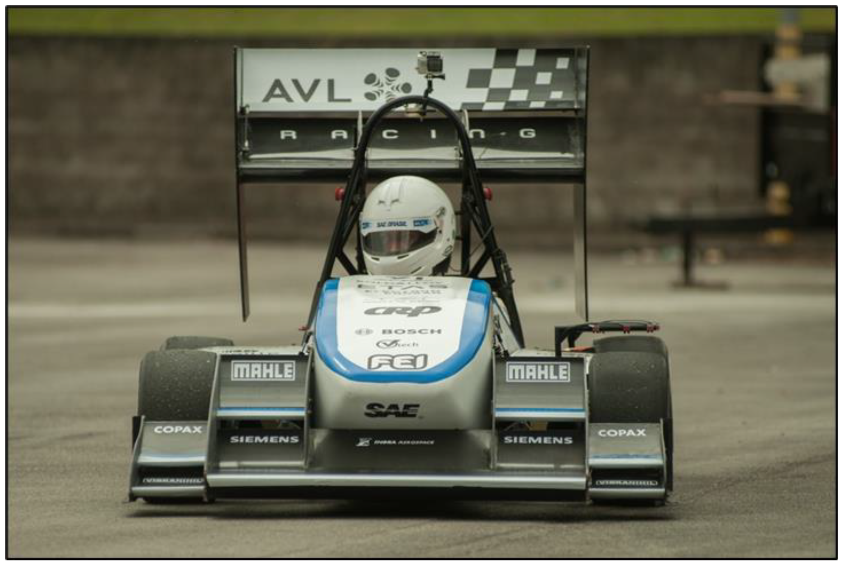
The reference is a fully electric vehicle prototype used in the Formula SAE competition, as shown in
Figure 1, named by the team as the Formula FEI TV vehicle. The permanent magnet synchronous motor (PMSM) used is from EMRAX. The motor has 86 kW power pick and 56 kW in the continued operation. The torque is amplified by a 4.4:1 fixed planetary gear, resulting in 877 Nm at the rear wheels.
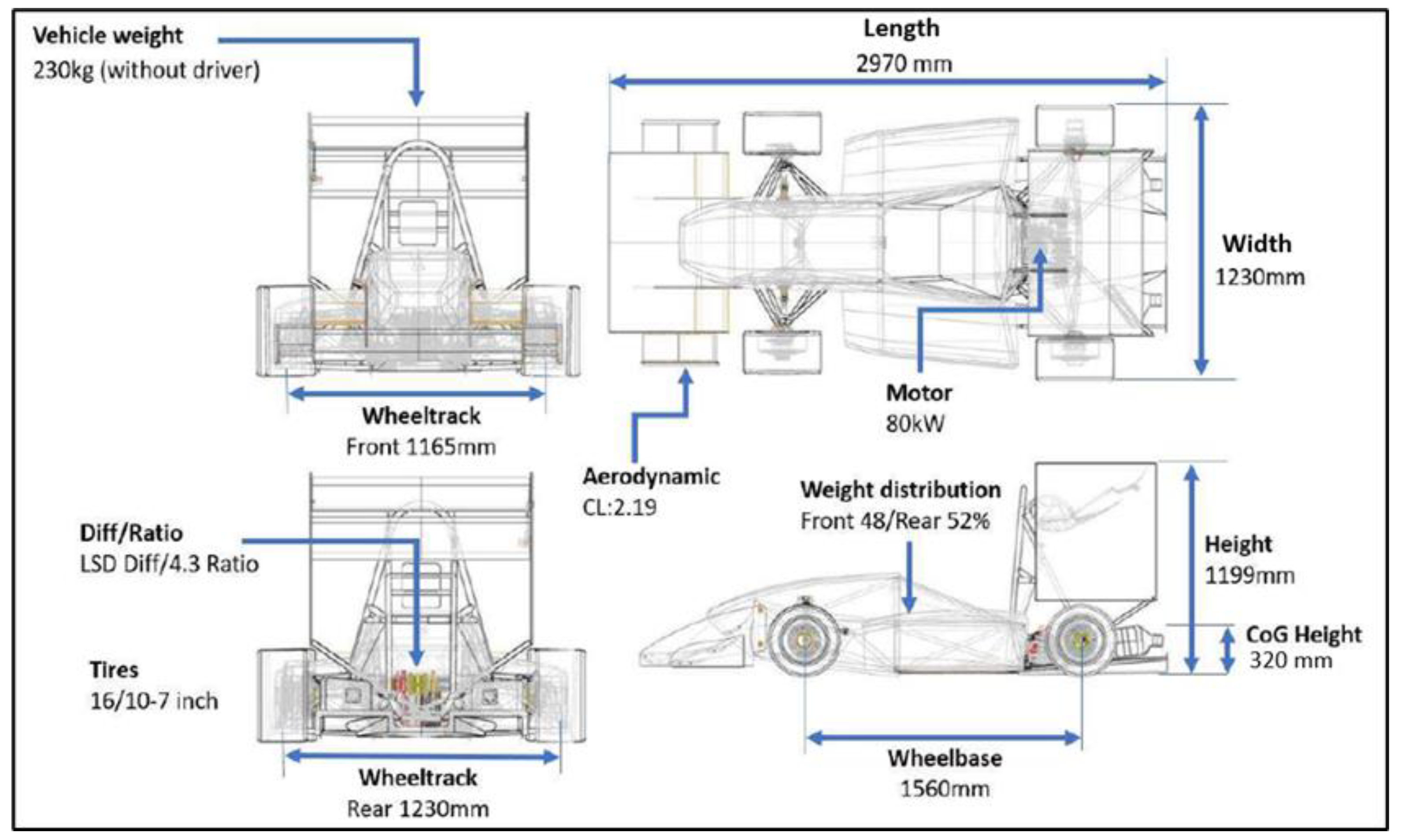
Figure 2 presents the primary vehicle parameter data utilized as input for the simulator.
2.2. Experimental Setup
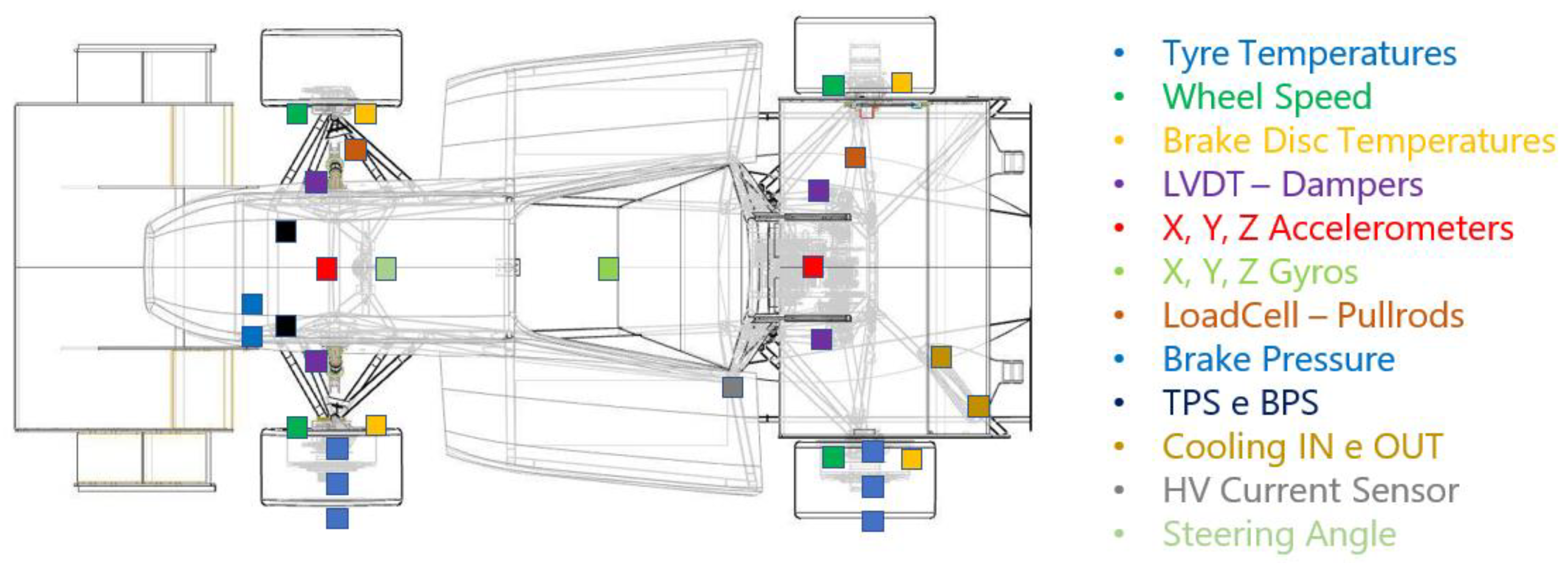
Several types of sensors were used for vehicle instrumentation, among them the following: tire temperature; wheel speed; brake disc temperature; accelerometer for measuring lateral, vertical, and longitudinal vehicle dynamics; Linear Velocity Transducer (LVT) dampers; brake pressure; steering angle and high voltage current sensor.
Figure 3 shows the car drawing to indicate the sensors’ position. For data acquisition, the Enclosed data Logger (EDL3) from MOTEC was used, which is a fully programmable data logger able to record up to 1000 samples per second. The GPS module provides accurate information about the car’s position on the track. This allows for the simultaneous recording and proper storage of all sensor measurements based on the car’s correct position on each lap of the track.
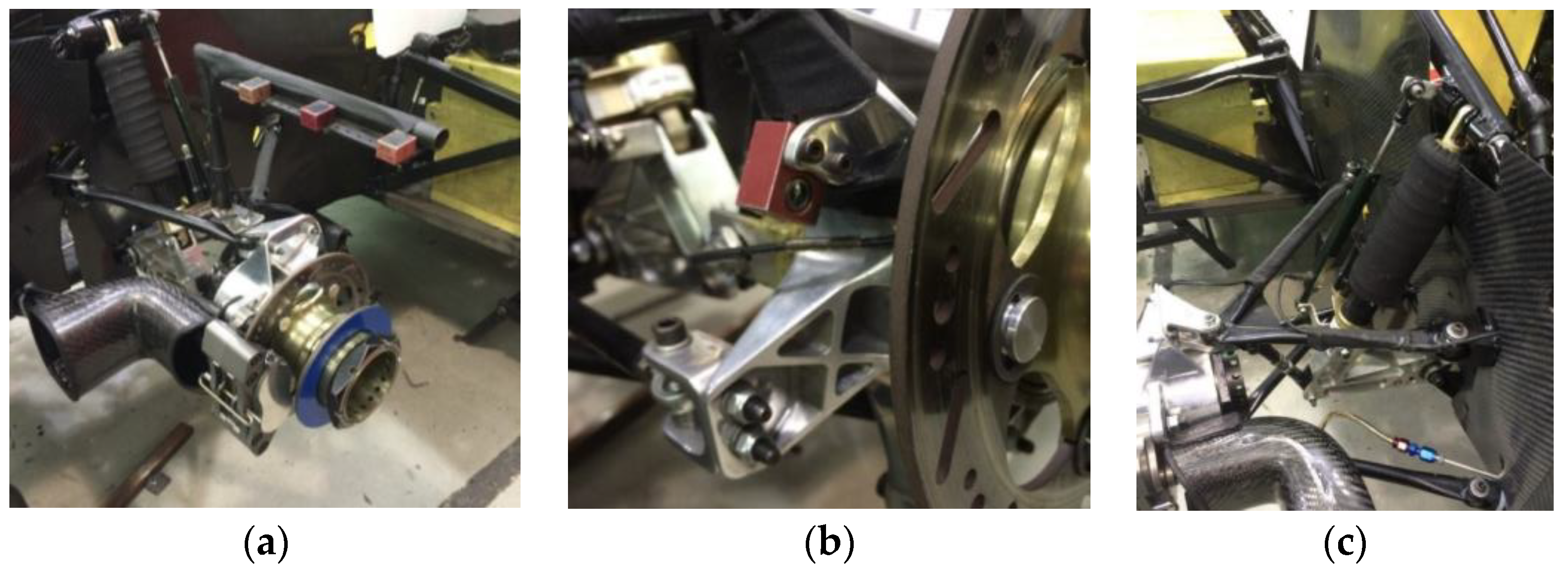
Figure 4 displays images of the sensors integrated within the car, encompassing (
Figure 4a) a sensor designed to measure tire temperature; (
Figure 4b) a sensor dedicated to monitoring brake disc temperature; and (
Figure 4c) a sensor employed for quantifying suspension displacement. In
Table 1, it is possible to visualize the sensors utilized and their respective brands and models.
2.3. Simulator and Modeling
Simulation of a complete vehicle, with accurate data of longitudinal, vertical, and lateral acceleration with a non-linear multibody approach, requires a precise tool, as used in automotive industries because they need to reduce prototype numbers and development tests. Therefore, the tool used in this study was the AVL VSM 4™ as it can simulate our vehicle consistently and be combined with AVL-DRIVE 4™ for objective vehicle assessment [
25].
The Formula FEI TV vehicle was designed using a multibody simulation approach, considering the maximum power that can be transferred from the battery to the powertrain, capped at 80 kW. The decision to employ either a single or four motor depends on optimizing the available maximum power concerning the performance required for specific track maneuvers dictated by the competition. The utilized software takes input data from the vehicle and configures the driver model through a feed-forward controller. All simulations are conducted in the steady-state regime, ensuring that tire behavior remains within the linear range, thereby eliminating transient maneuver effects.
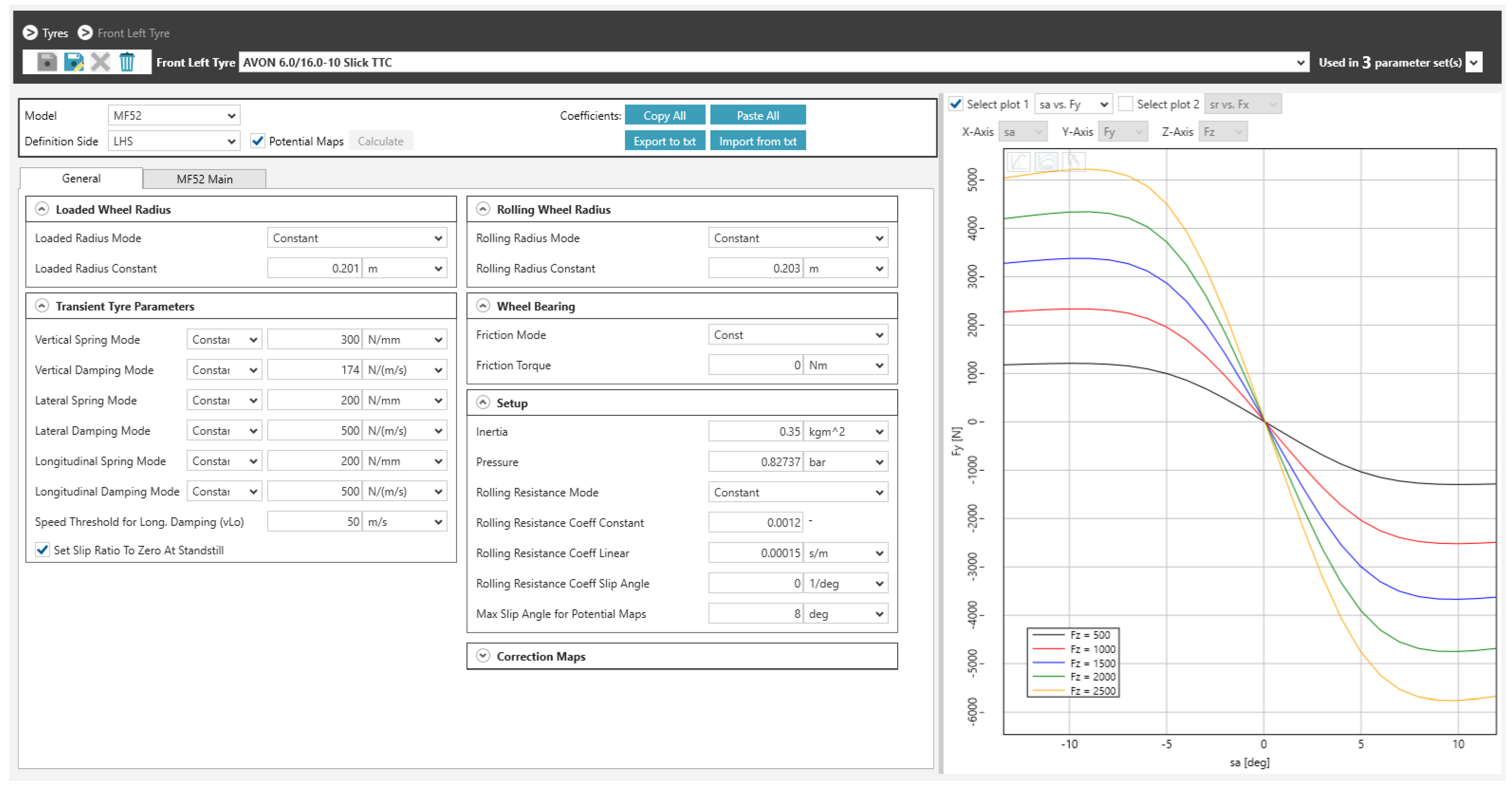
2.3.1. Tire
In the multibody tire system model, the tire’s dynamic measurements were utilized and compared to data obtained from laboratory tests. Typically, these parameters are provided by the tire manufacturer and contribute to creating a maximum lateral force graph for the tire based on the steering wheel’s slip angle, commonly referred to as the drift angle. This graph allows for extracting all dynamic tire coefficients imported into the AVL VSM software. The software processes these coefficients during the simulation’s pre-processing phase, defining the traction limits and tire saturation for lateral and longitudinal forces. Ultimately, these post-processed coefficients serve as input parameters in the multibody model, as shown in
Figure 5.
2.3.2. Suspension and Steering: Kinematic Gains
The suspension and the steering system are simulated in the AVL VSM environment to obtain the kinematic data regarding the geometric gains of the system. To achieve this, coordinates are integrated into the program, generating the kinematic curves for Camber and Toe gains based on defined movements and oscillation frequencies. To establish the initial static kinematic gains, the suspension and steering modeling process involves utilizing coordinates for all suspension points, assisted by dedicated kinematic software such as Optimum Kinematics 6.11.
The front suspension exhibits a vertical travel of 35mm, (20 mm for compression and 15 mm for rebound). When a positive vertical displacement occurs on the wheel, it leads to an inclination angle increase.
All kinematic gains are incorporated into the multibody model, ensuring that the kinematic effects are accurately considered. These parameters are subsequently integrated into the AVL VSM software for further analysis and evaluation.
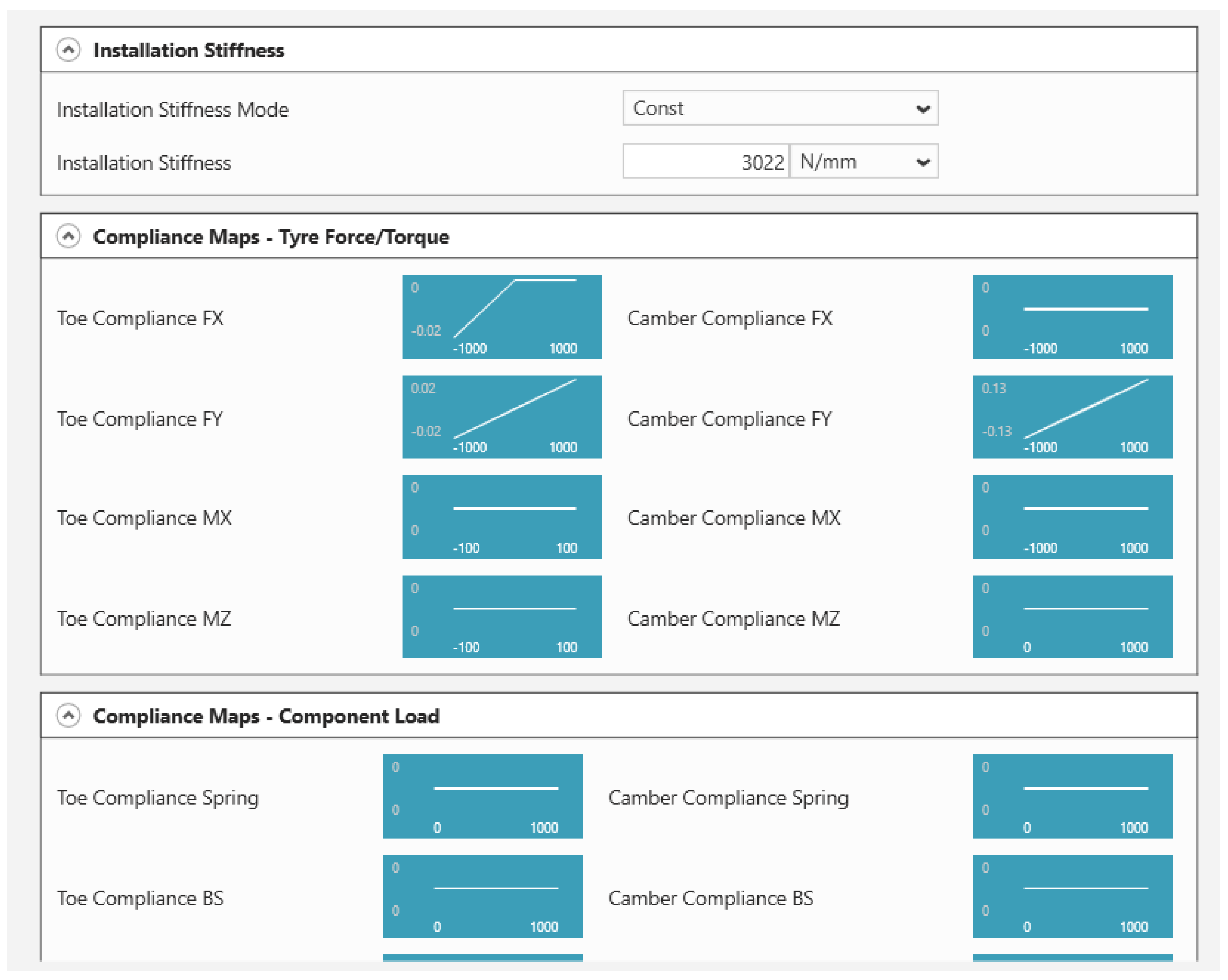
2.3.3. Suspension and Steering: Elastic Gains
In addition to the kinematic gains, we also have the Kinematic Compliance. To measure these gains, a mechanical device capable of applying defined lateral and longitudinal forces was developed, and measurements of convergence and tilt gains were taken.
Figure 6 shows the AVL VSM software screen displaying the extracted experimental elastic gains from the Formula FEI TV vehicle.
2.3.4. Dampers and Springs
Responsible for controlling the tire-to-ground contact, dampers play a crucial role in the model correlation. To achieve this, two types of isolated measurements were performed: one externally to the vehicle (Damper Dyno) and one on the vehicle during empirical tests to create the characteristic damper curve. The dampers used are Ohlins 7800, which offer independent compression and rebound adjustments. This allowed for the implementation of the parameters in the multibody model. It is important to note that the dampers used have 21 adjustment combinations. To ensure greater consistency in the correlation results, only one mode was chosen and used throughout all the tests.
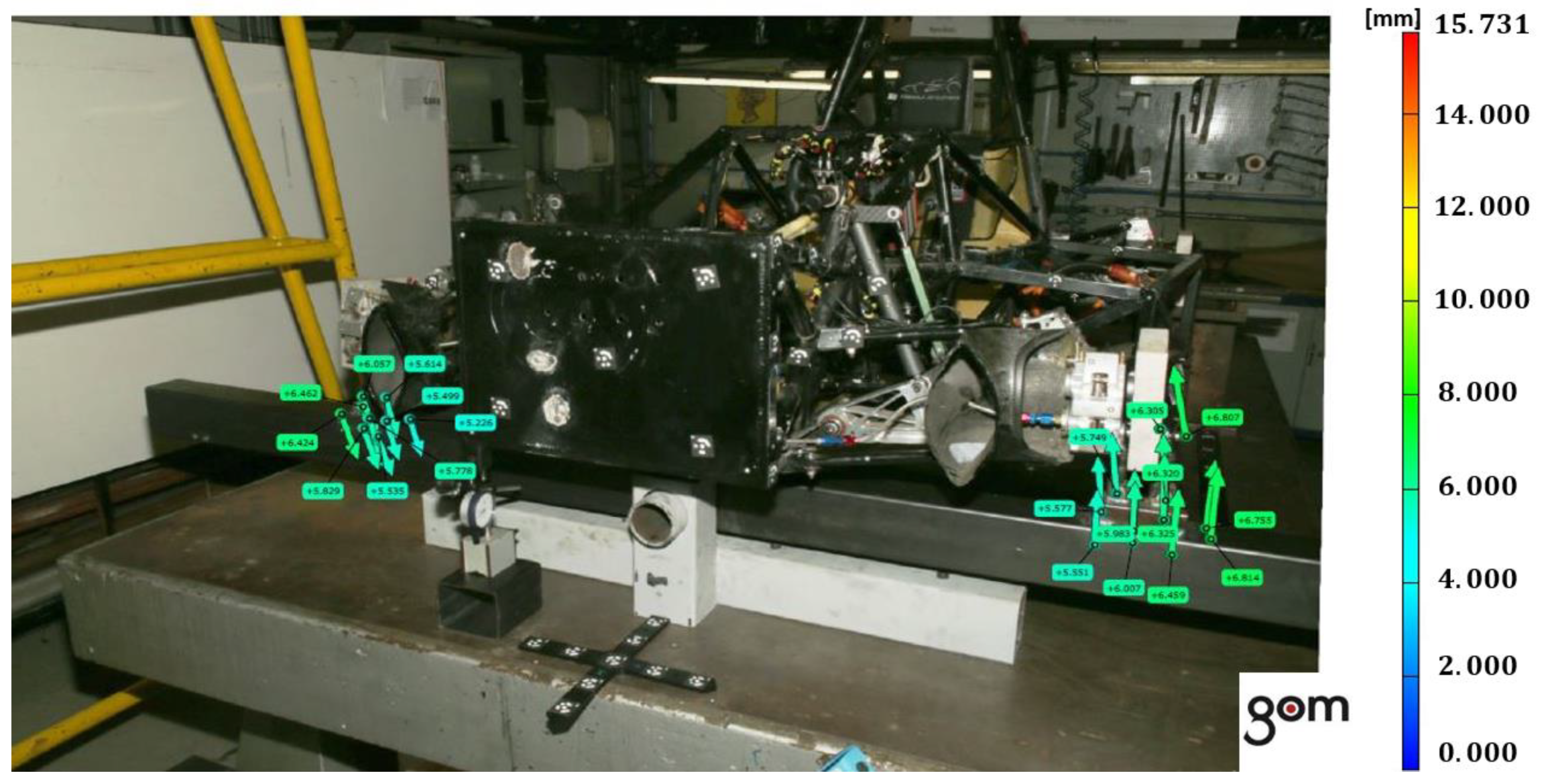
2.3.5. Chassis
For this multibody analysis, the chassis was modeled using its torsional stiffness, obtained through photometry and the coordinates of the center of gravity [
26]. The method involves raising one of the vehicle’s axes and, based on the height of the lift and the variation in mass on the axes (measured using scales on each wheel), calculating the height of the vehicle’s center of gravity.
The measurement of the center of gravity height should be performed with the suspension and tires in a condition of maximum rigidity to eliminate the variation caused by the elastic elements of the suspension. Therefore, the dampers are replaced with rigid elements, and a higher tire pressure than the reference of 12 psi is used.
Following the chassis modeling, the measurement of the complete assembly’s torsional stiffness was carried out, including the elastic elements of the suspension. In collaboration with VTech, a process utilizing photometric analysis of defined points on the chassis was employed to evaluate the torsional stiffness. With the collected data, it was possible to implement the torsional stiffness model into the AVL VSM software, as presented in
Figure 7.
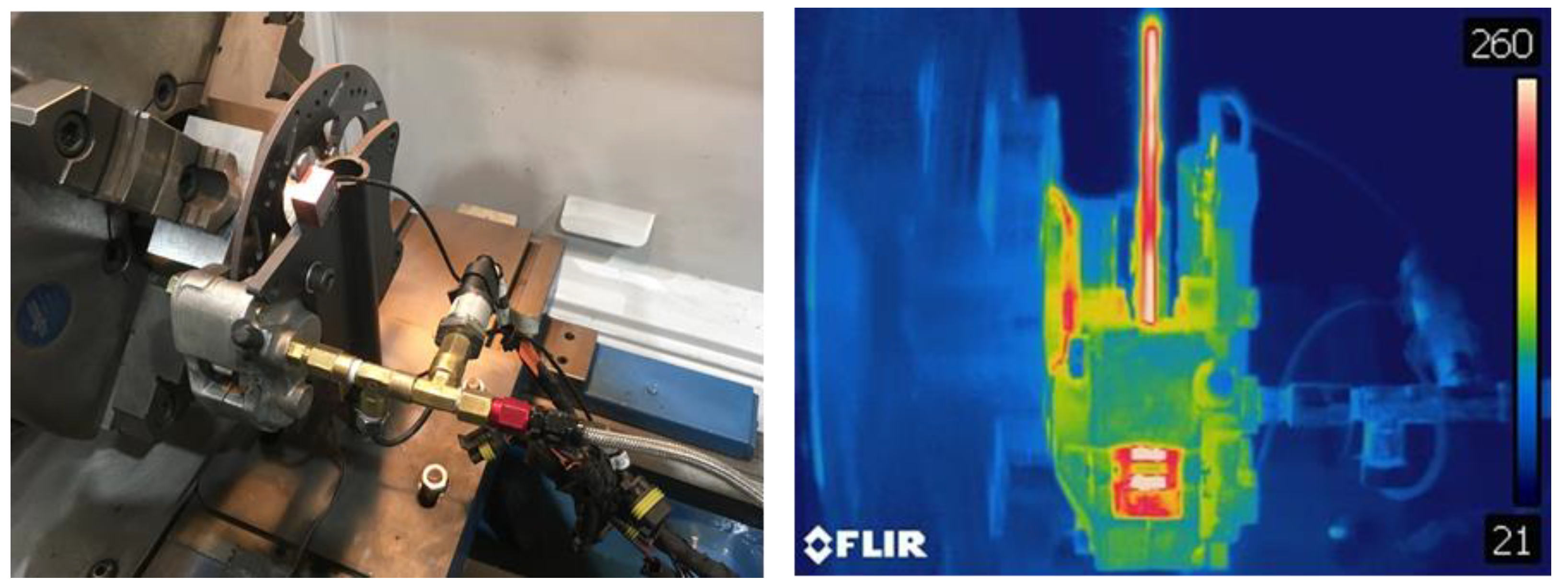
2.3.6. Brake Pads
The friction coefficient of the brake pads with the disc was extracted with the aid of a brake dynamometer, as presented in
Figure 8. The test involved instrumenting the brake caliper mounting system, along with measuring temperatures and pressure in the brake line. Based on the test, it was possible to determine the operating range of temperatures and friction coefficients for the front and rear brake pads.
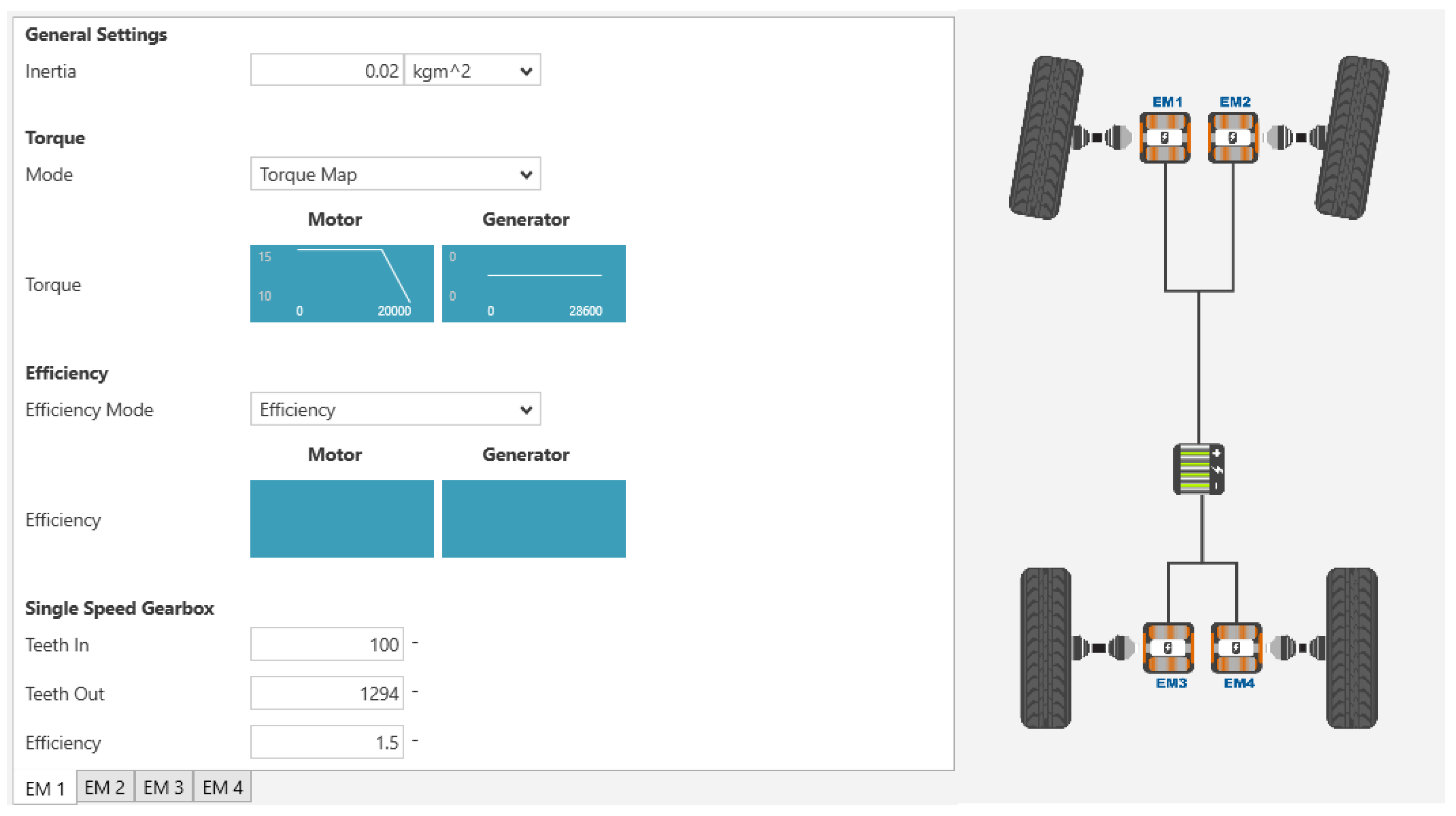
2.3.7. Powertrain
To gather data on the electric powertrain, dynamic measurements were taken on a roller dynamometer to determine the torque demands for each acceleration condition based on the estimates provided by the electric motor controller. By analyzing the torque demand, which can be inferred from the electric current used, it was possible to acquire data on the electric powertrain. Vehicle data acquisition was utilized, as the torque request signals from the inverter and speed are available and compared with the torque, power, and efficiency data provided by the manufacturer. These data were collected during a lap on the test circuit.
Figure 9 presents the AVL VSM software indicating powertrain parameters.
2.3.8. Aerodynamics and Resistive Forces
In the development of the vehicle’s computational model, the coefficients of resistive forces were considered, obtained from a test called CoastDown, aiming to closely replicate the pattern specified by ISO 10521-1:2006 [
27], which specifies the measurement conditions and test procedure.
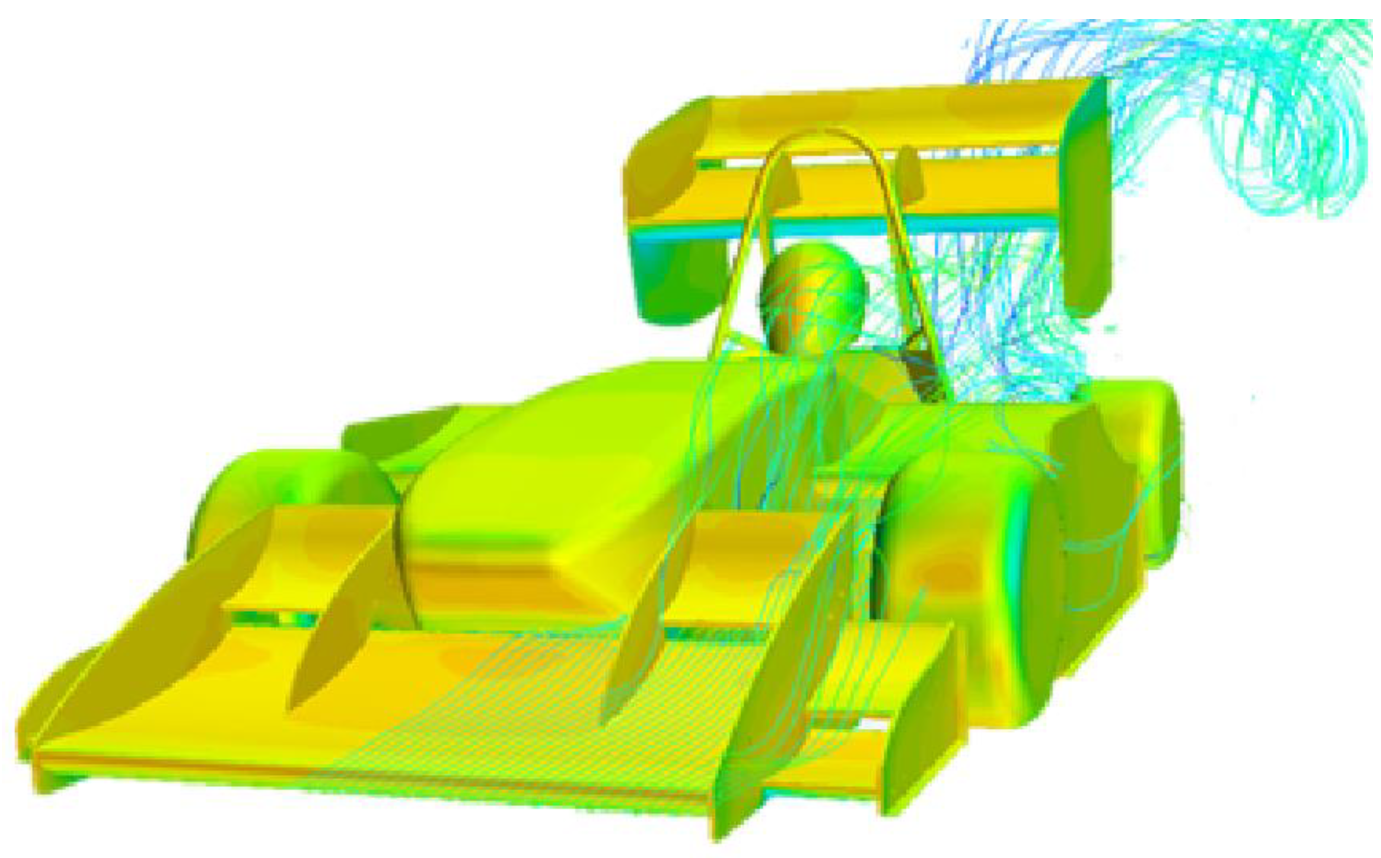
In addition to the aerodynamic resistance model, a Computational Fluid Dynamics (CFD) analysis was conducted using a 3D scanned model of the actual vehicle and is presented in
Figure 10. With the scanned model, CFD was performed using the StarCCM+ Adapco software [
28] to obtain the aerodynamic map, which represents the drag and downforce coefficients based on the variation of the vehicle’s front and rear heights. This parameter is highly sensitive for dynamic model correlation.
2.4. Control Strategy
The default control method used by the AVL VSM 4™ software considers the PID (Proportional Integral Derivative) controllers regulate base. The concept of individual torque control using feedback through a Proportional-Integral (PI) control loop is a fundamental aspect of achieving precise and accurate control over the motion and behavior of each Individual Wheel Module (IWM).
Appendix A presents the control strategy math modeling in equations A1 to A26. This control methodology enables the IWM system to respond dynamically to changing conditions and adapt its torque output accordingly [
29,
30]. The Proportional-Integral (PI) control loop is a widely used control algorithm that combines two essential components: proportional control and integral control. The proportional control component considers the difference between the desired reference torque and the current torque and adjusts the output torque proportionally to minimize this difference. This allows the IWM to respond quickly to changes in the desired torque and maintain a desired speed.
The integral control component of the PI control loop addresses the accumulation of any persistent error between the desired torque and the actual torque over time. It continuously integrates this error and applies corrective measures to eliminate the accumulated error. By incorporating the integral control, the system can effectively compensate for any steady-state errors and ensure accurate torque delivery.
By utilizing this feedback-based control approach, the IWM system can continuously monitor the torque load on each wheel and adjust the torque output accordingly. This real-time estimation of torque load is crucial for maintaining traction and optimizing performance on different road surfaces and varying load conditions. For instance, if the road grip diminishes due to weather conditions, the individual torque control system detects this change through the feedback loop. It then automatically reduces the torque output for the affected wheel, preventing excessive wheel slip and enhancing overall stability and control. Similarly, suppose there is an increase in the vertical load on a particular wheel, such as during cornering or weight transfer. In that case, the control system can respond by increasing the torque output to ensure sufficient traction and stability.
2.5. Maneuvers Definition
To validate the controller, some maneuvers must be evaluated so that the team can analyze the longitudinal and lateral dynamics separately. Therefore, the sequence below was defined: Acceleration, Coastdown, Skidpad, and Autocross [
31,
32,
33,
34,
35]. The acceleration maneuver is performed with the vehicle starting from rest, and the pilot instantly accelerates 100% of the accelerator pedal. In this maneuver, in addition to providing important information on the profile of the speed increase as a function of space, the entire drive wheel traction system is tested by describing the general behavior of the vehicle’s longitudinal dynamics.
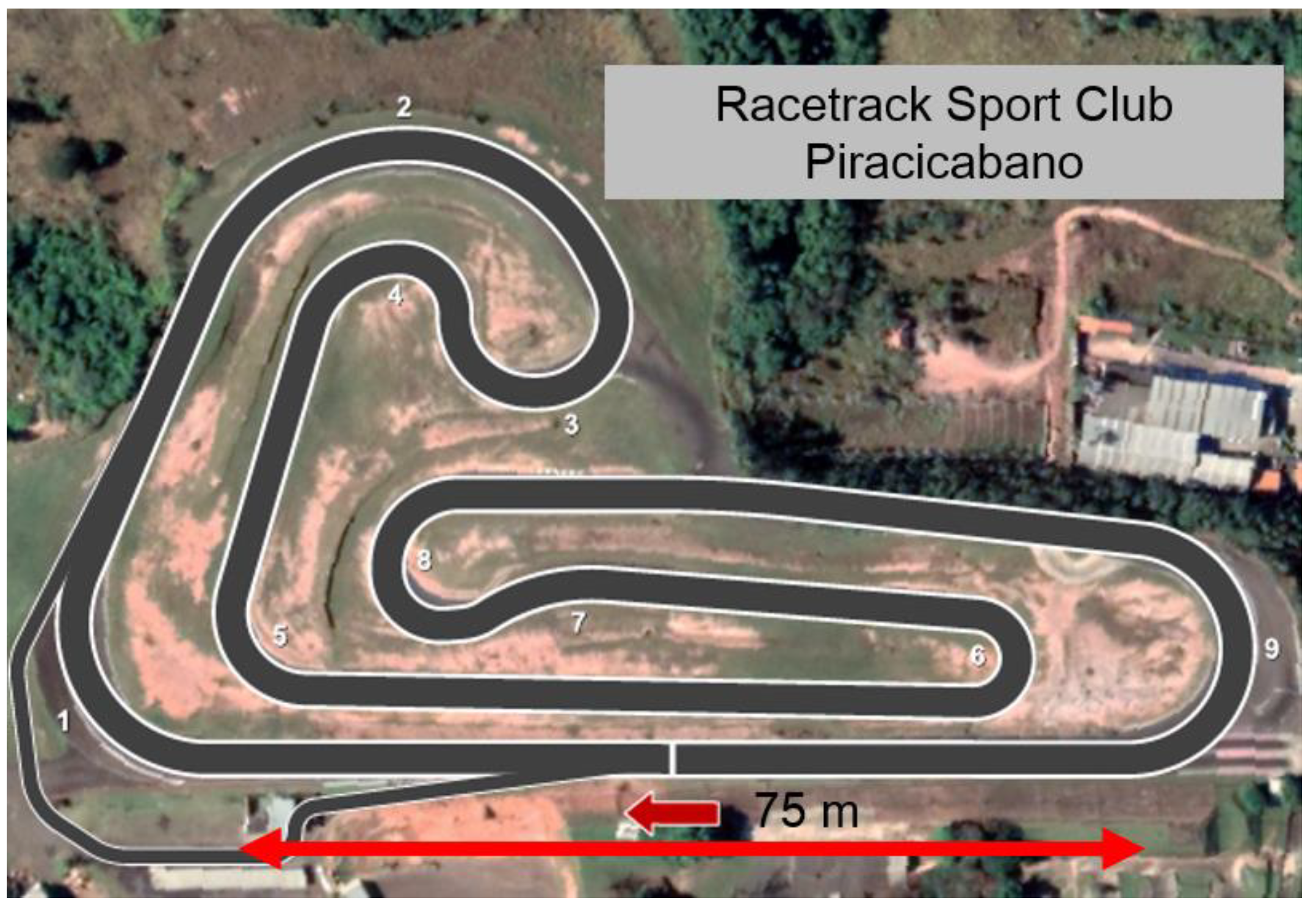
Coastdown is widely used in the automotive industry to measure the vehicle’s deceleration profile. It has an analysis capability to measure the speed decay profile, covering resistive forces to rolling, friction, and profile aerodynamics. Both maneuvers were conducted in the Racetrack Sport Club Piracicabano (ECPA, São Paulo, Brazil) circuit, as shown in
Figure 11. It is the same place where Formula SAE Brazil competitions have been held for the last ten years.
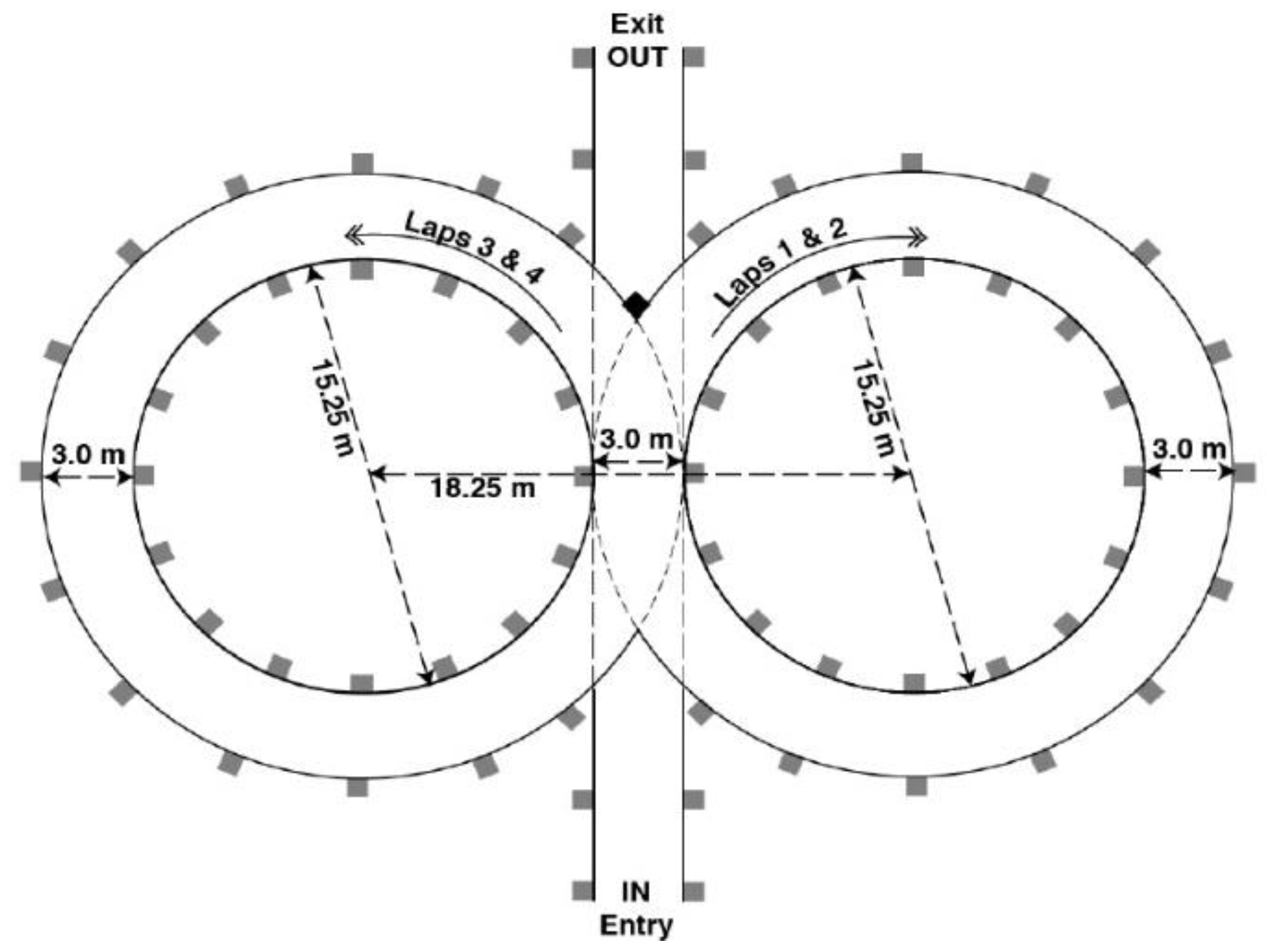
Skidpad, this maneuver can measure the lateral acceleration of the vehicle. It is a maneuver that brings together two circles next to each other, forming an 8-figure, where the vehicle performs two turns to the left and two more to the right. According to the competition rule, the maneuver must follow the configuration shown in
Figure 12. The parking lot at FEI University was used for this analysis.
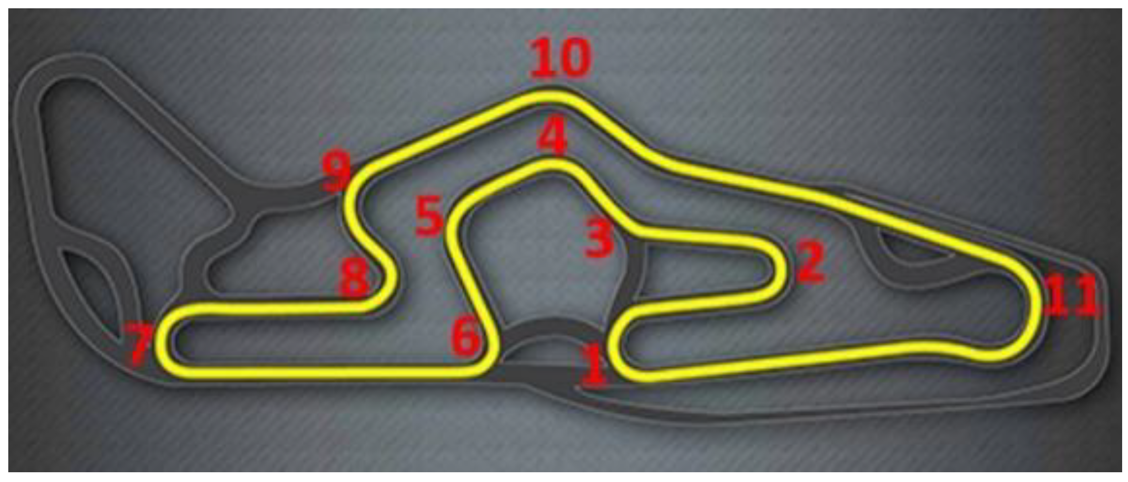
Finally, the Autocross is a fast lap on a given circuit. The vehicle must demonstrate its maximum capability to cover a lap of approximately 1 km in the shortest time possible. The Interlagos track (São Paulo, Brazil) was chosen, in which the team performed a practice session with the vehicle fully instrumented. The layout can be seen in
Figure 13 and has a total length of 900 m. It has been divided into 11 curves (indicated in the picture below in red), 1 long straight, and 2 shorter straights, to understand better the vehicle’s exact location, which facilitates the identification of the vehicle’s behavior in each situation.
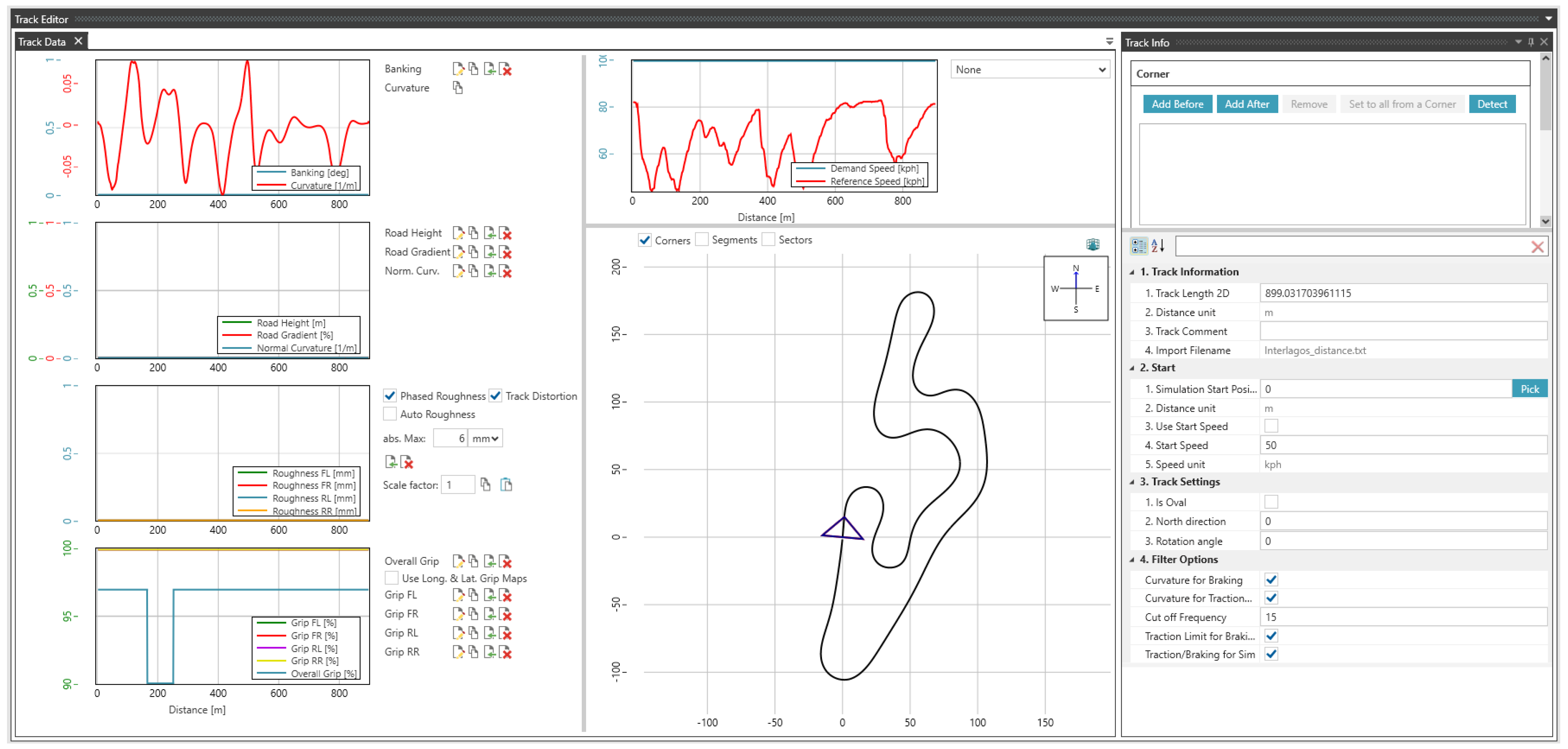
The track modeling used vehicle sensor data, including GPS and accelerometers, to characterize the test track. Based on the coordinates generated by the acquisition system, it is possible to generate the track using computational geolocation and terrain analysis tools, such as Google Earth Pro. This allows the AVL VSM program to capture the X, Y, and Z coordinates referenced from the Latitude, Longitude, and Altitude coordinates acquired via GPS.
Figure 14 presents a detailed representation of the racetrack generated by the software. The track’s circuit, curves, straight sections, and elevation changes are captured. The GPS and accelerometer data coordinates were used to create this model, enabling geolocation and terrain analysis for optimal racetrack design and simulation.
3. Modeling Results
3.1. Acceleration
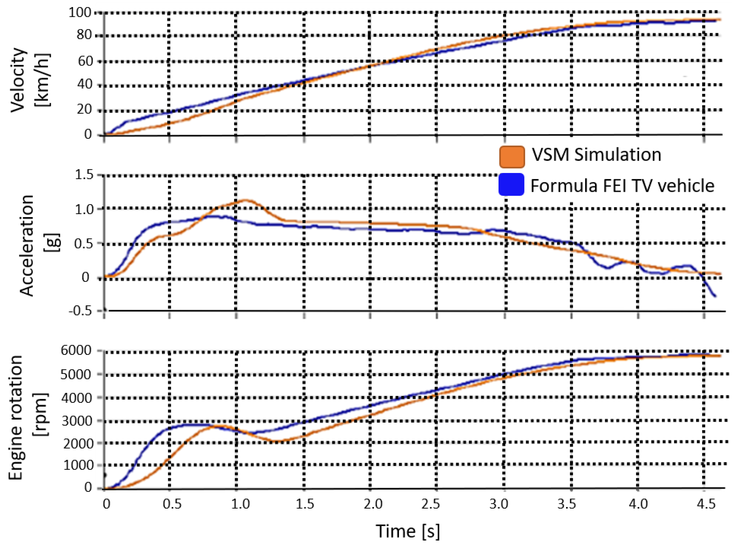
The Formula FEI team consider the acceleration maneuver, one of the most important dynamic tests in the competition. Due to constancy in this training, the team has good knowledge and practice in performing this type of maneuver. As a result, this test has very reliable results from the point of view of numerical values of acceleration and velocity, as presented in
Figure 15. The velocity profile has a similar trend between the simulation and the test. However, there is a small difference at the beginning of the maneuver. This difference is caused by the slipping of the wheels at the very beginning of the vehicle’s movement. The real test car did not have traction control, so even with the most experienced drivers there is usually a slight slip at the start of acceleration. Regarding acceleration values, the profile of the two curves also presents similar trend between simulated and real. The same slipping of the wheels in the initial part of the movement is observed. Lastly, concerning engine rotation, it was expected that engine rotation would be higher in the initial part of the vehicle movement due to the slip in the actual test. This fact demonstrates the great sensitivity of the data acquisition equipment used by the team and the good accuracy of the AVL VSM simulation software.
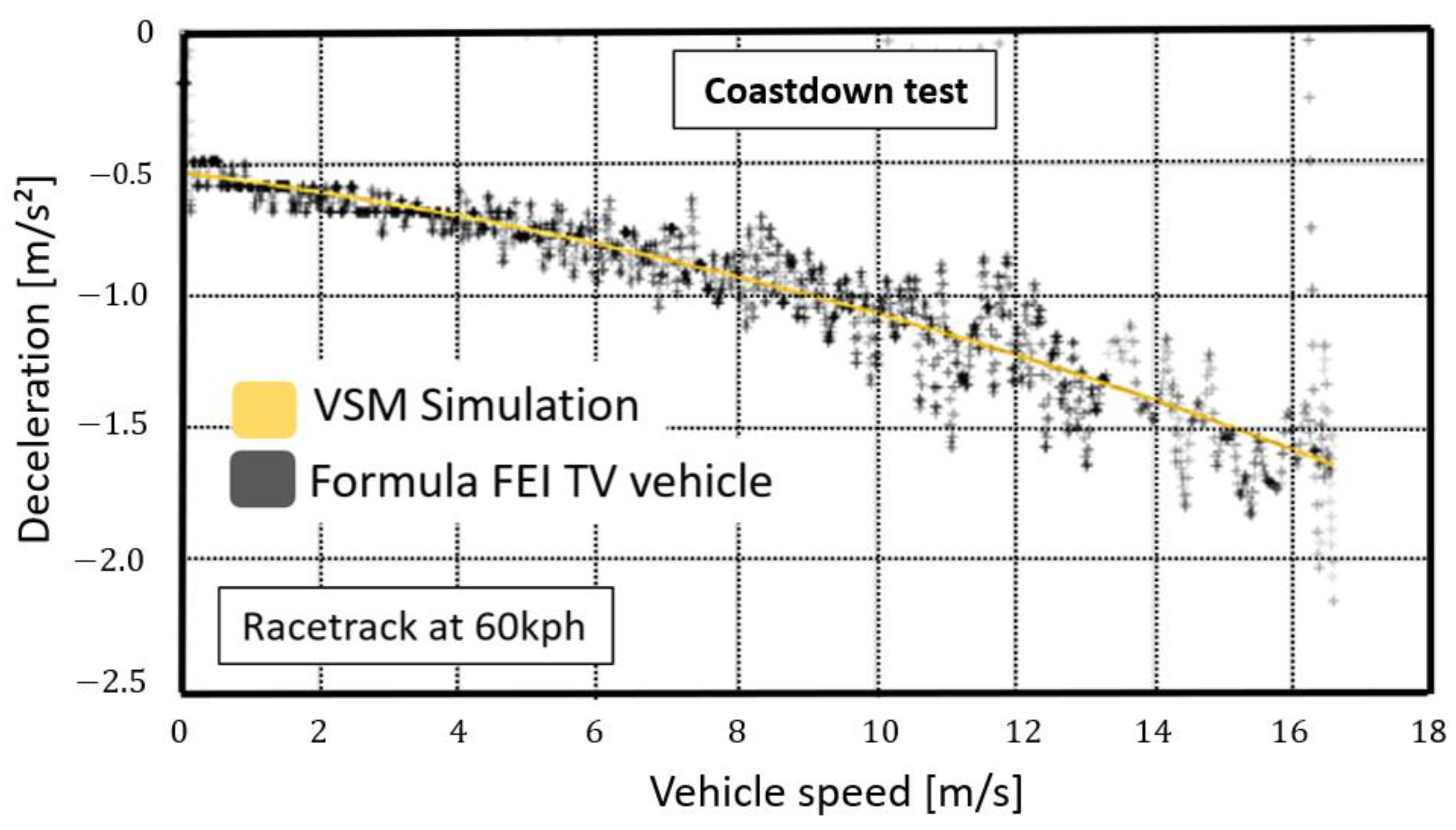
3.2. Coastdown
The track on which the car would perform most of the tests was chosen, as there is some sensitivity concerning the type of pavement, in this case, the circuit’s asphalt. The speed at which the vehicle started the test adopted by the team was 60 km/h. The definition of this speed was due to the length of the straight line not being wide enough to perform maneuvers at higher speeds.
Figure 16 presents the deceleration curve as a function of the vehicle speed, and it is possible to observe the data correlation between track and simulation in the AVL VSM software. The velocity decay and longitudinal acceleration profiles were very similar, obtaining a good correlation between the mathematical model and the test performed on the track.
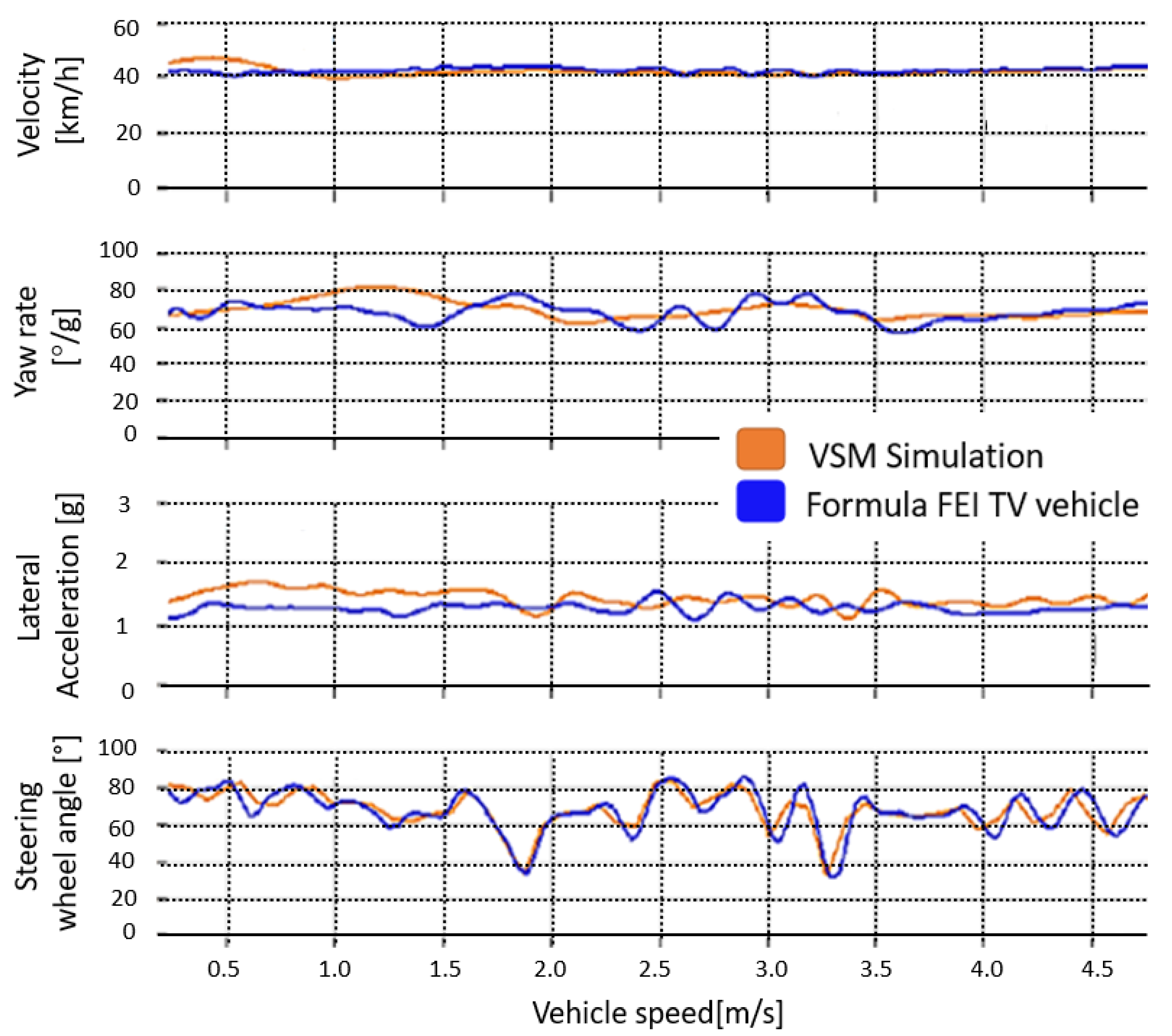
3.3. Skidpad
According to
Figure 17, the correlation between various quantities, such as vehicle speed, yaw rate, lateral acceleration, and steering wheel angle, was very close during the steady-state maneuver. At
Appendix A.4 it is possible to observe the steer Gradient dependence on the Yaw Rate performance, according to Equation (A25). This maneuver involved finding the maximum speed the vehicle can maintain while navigating a curve with a constant radius. The steering wheel angle is crucial in understanding the vehicle’s behavior during the maneuver. In this case, the steering angle needed to be reduced to correct for oversteering, which is a common issue that drivers face while performing such maneuvers. The results were satisfactory and indicated a good understanding of the vehicle’s behavior during the steady-state maneuver.
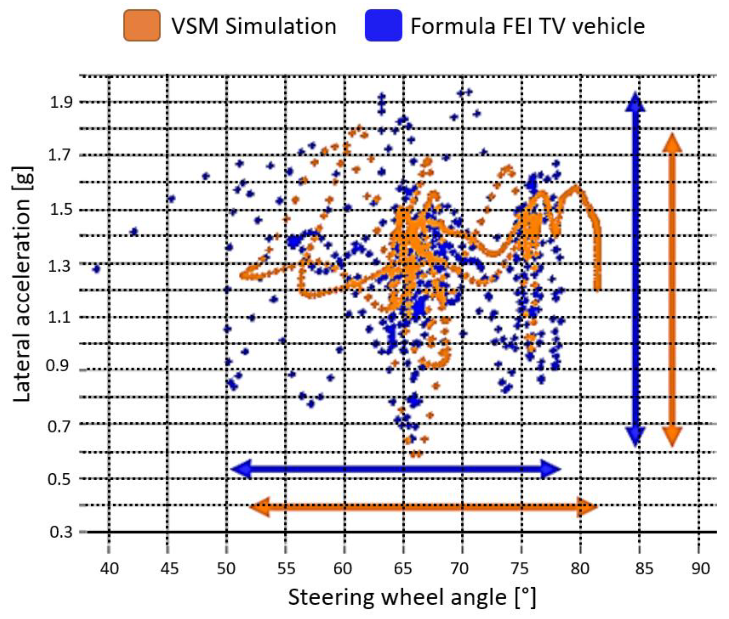
Figure 18 presents the lateral acceleration diagram as it relates to the steering angle of the steering wheel. It shows how much the driver must steer the wheel to increase the vehicle’s lateral acceleration, and it reflects the relationship between the tire grip on the road, suspension kinematics, and the linearity and response of the vehicle’s steering system. It is usual to observe isolated data points in actual test measurements due to the sensitivity of the sensors installed in the vehicle.
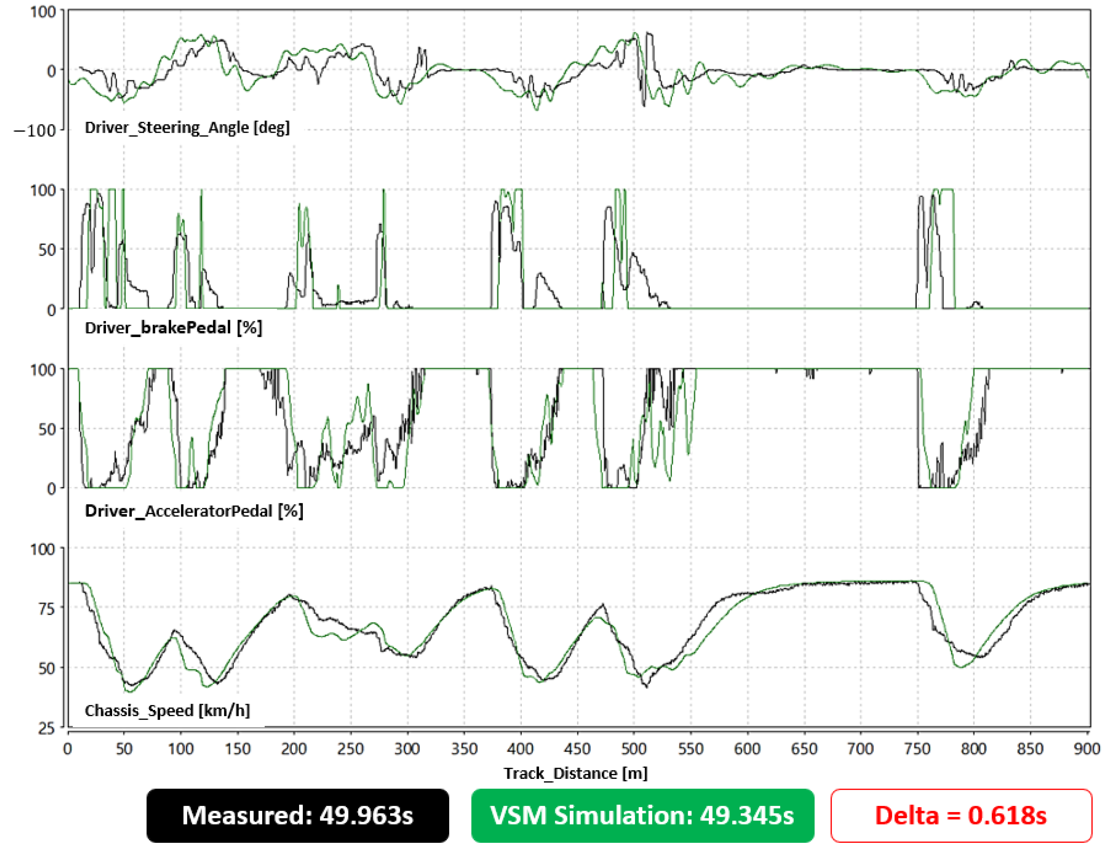
3.4. Autocross
Figure 19 presents the most critical information of all this modeling: the time it takes the vehicle to cover a lap in the Interlagos circuit. In this case, the actual on-track measurement was 49.963 s, and the simulation in the AVL VSM software was 49.345 s, which brings a difference of only 0.6 s.
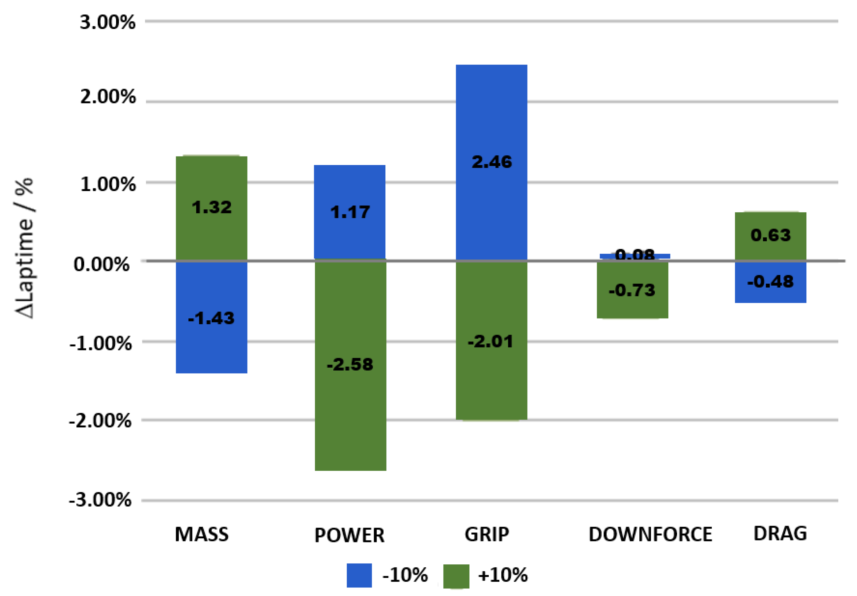
Based on the data obtained in this simulation, a sensitivity analysis of the model was applied to understand the degree of reliability. The purpose of this analysis is to make some considerable changes in some factors that are usually quite sensitive. Some examples are mass, power, frontal area, grip, and aerodynamic force that pushes the car against the ground (Downforce).
Figure 20 presents whether to increase or decrease each parameter of those mentioned in the order of +/−10%. It is interesting to note that the two factors that most influence the optimization of the lap time are engine power and grip.
4. Torque Vectoring in the 4WD Model
The default control method employed for the 4WD (four-wheel drive) vehicle is designed to be comparable to that used for the 2WD (two-wheel drive) vehicle [
25], enabling an initial fair comparison. Despite its simplicity, this approach has yielded some noteworthy preliminary results. Each rear wheel has a controller for torque vectoring. The torque vectoring system employs a proportional-integral-derivative (PID) control with weightings based on variations in measurements at each wheel, which the software provides. The torque vectoring system in the two-degree-of-freedom (2-DOF) vehicle model is a pivotal component that significantly influences the vehicle’s stability, control, and handling characteristics. The system operates based on the modified Equation (1):
In this equation, ∆T represents the delta torque of the rear axle, which is the difference in torque between the left and right wheels. The variables k1, k2, k3, and k4 are coefficients that determine the weighting or sensitivity of each input. These coefficients are adjusted to achieve the desired handling characteristics, responsiveness, and stability based on the specific 2-DOF vehicle model and the torque vectoring system employed.
∆α represents the variation in slip, with a reference value of 1 indicating no slippage. It compares the wheel speed with the vehicle speed and how much the left or right wheel loses traction. M represents the desired yaw moment, the moment of the vehicle’s vertical axis. δ represents the steering wheel angle.
This system recognizes the importance of considering the rate at which the slip angle difference changes, which can influence torque distribution, improving stability and control. This is the derivative portion of the control. Furthermore, the accumulated error is acknowledged as an essential aspect, representing an integral part of the control.
The PID controllers utilized in the study employ default software constants that have yet to be optimized. The control strategy will improve significantly once the initial 4WD prototype becomes available, but the results obtained so far show a great potential to enhance the vehicle’s performance.
Four-Wheel Drive Model Prediction
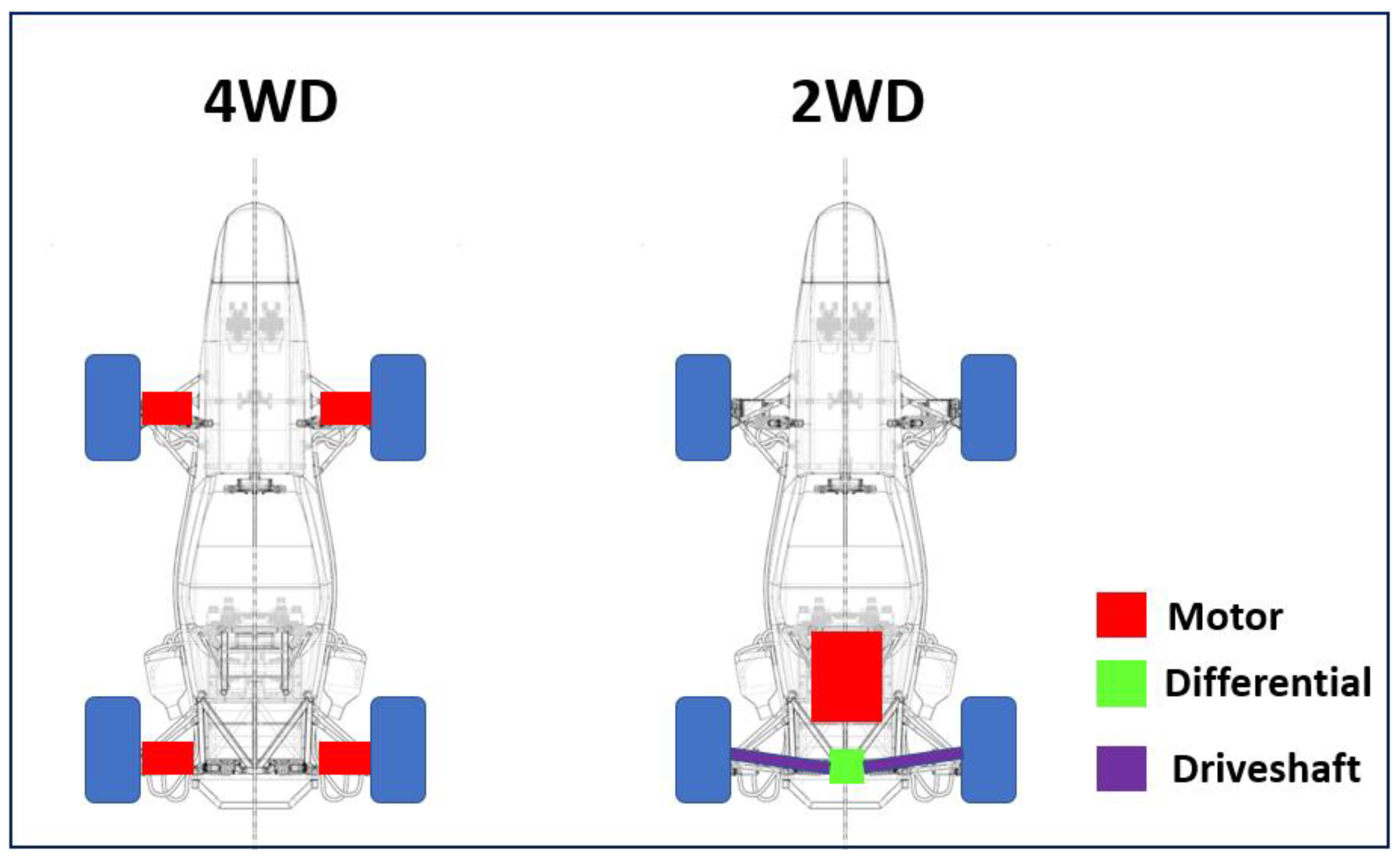
Once the simulation of a fast lap with good correlation is performed, it is possible to estimate the potential of the 4WD vehicle versus the 2WD vehicle presented in
Figure 21.
Some model-related changes were introduced starting from the 2WD Formula FEI TV vehicle. Four individual engines on each wheel replaced the unique rear engine. The differential has been removed, and consequently, each wheel can be controlled individually, both in traction torque and braking torque. The two lateral battery containers have been replaced by a central container at the rear, in the same position as the unique rear engine used to be. With this, the position of the center of gravity was changed, as well as the mass distribution between the axes. Another notable change involves increasing unsprung mass.
Unsprung mass is the mass that the damper spring assembly does not support. In vehicles, keeping the lowest level of unsuspended mass is always good, especially in racecar vehicles, as the collision of the wheels with the kerbs can cause a great disturbance in the steering wheel. In some more critical situations, the driver can lose control of the vehicle. However, in this specific competition, the application of Kerbs is rare. Therefore, they do not stand for much risk in this case for the drivers.
Figure 22 shows the first simulation result of the 4WD prototype in the AVL VSM software. It is essential to highlight that this simulation reduced lap time by approximately 7.5%.
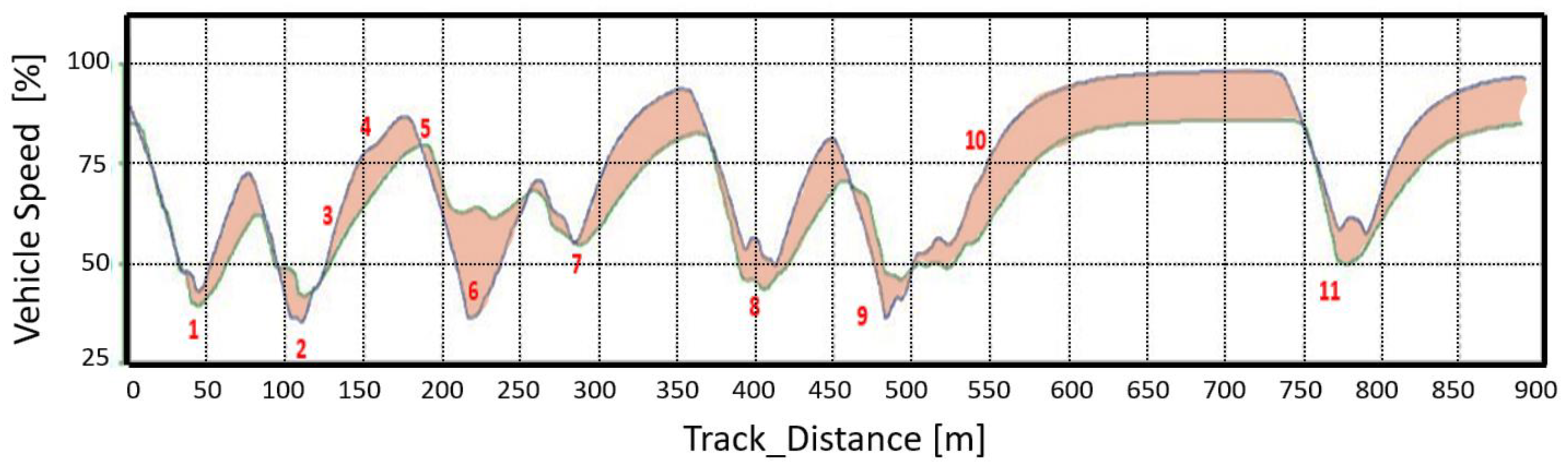
Considering the same previous speed profile, it is possible to see in
Figure 23 that due to the increase in power and traction capacity with the four engines, the area highlighted in orange represents the vehicle speed change with the swap to 4WD version, standing for the highest accelerations and consequently gains in lap time of Interlagos racetrack. The 11 corners are represented in red, according to the racetrack map previously explained in
Figure 13.
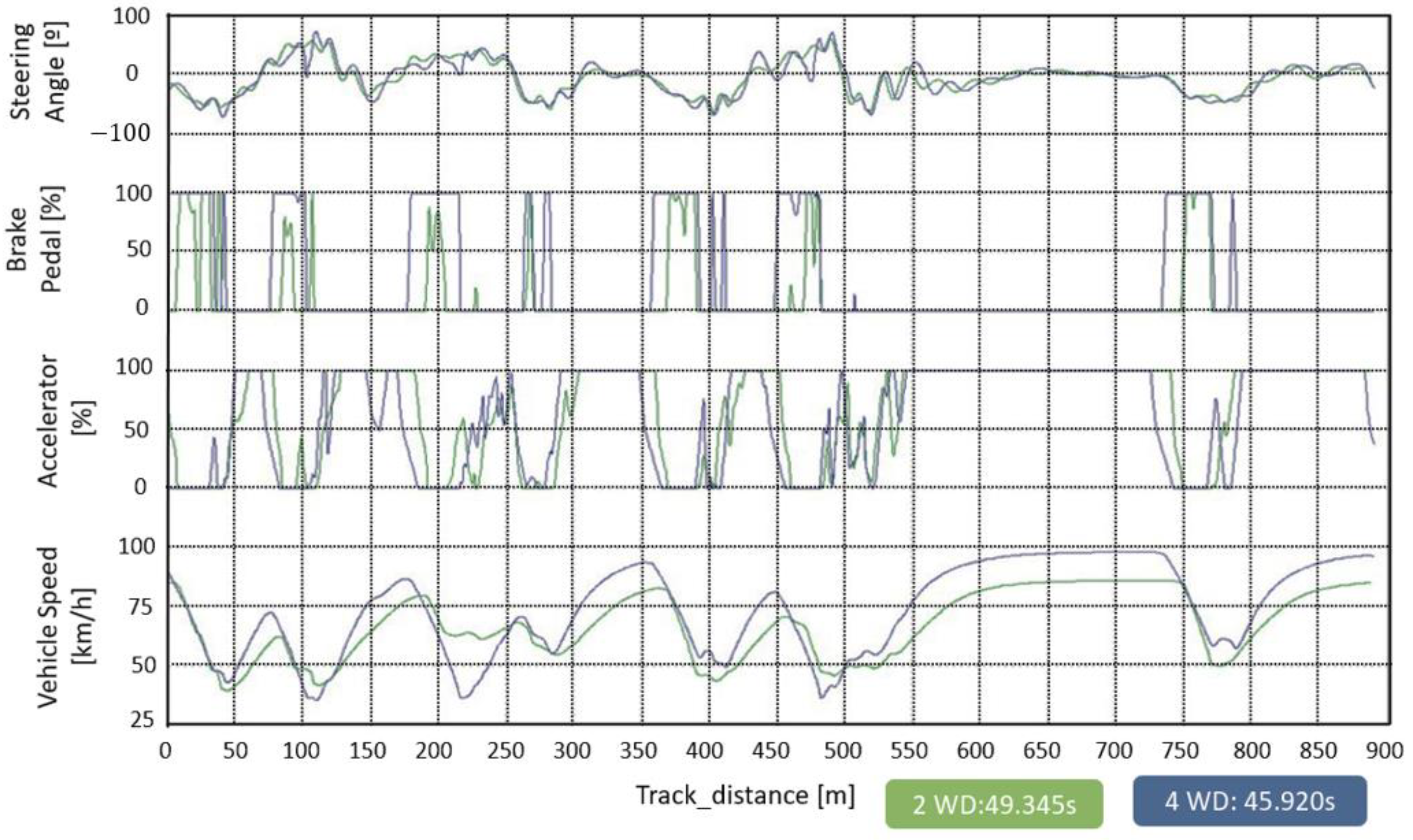
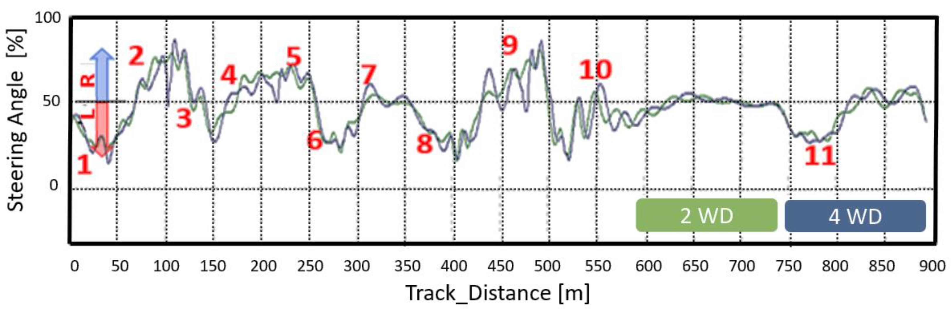
Analyzing the driver’s activities is crucial as it helps estimate the level of difficulty in controlling the vehicle. Three main indicators for this analysis are the steering angle of the steering wheel and the operation of the accelerator and brake pedals. When it comes to steering the wheel, it is important to note that a larger steering wheel angle indicates understeer behavior, where the front of the car tends to drift outward. Conversely, if the driver needs to reduce the steering wheel angle or steer in the opposite direction, it signifies oversteer behavior, where the rear of the vehicle tends to slide out. In terms of handling, both the 2WD and 4WD models exhibit similar behavior, as depicted in
Figure 24. This figure illustrates that the lateral accelerations and curve contour speeds remain relatively consistent for both vehicle types, regardless of low or high speeds, the 11 corners are represented in red, according to the racetrack map previously explained in
Figure 13.
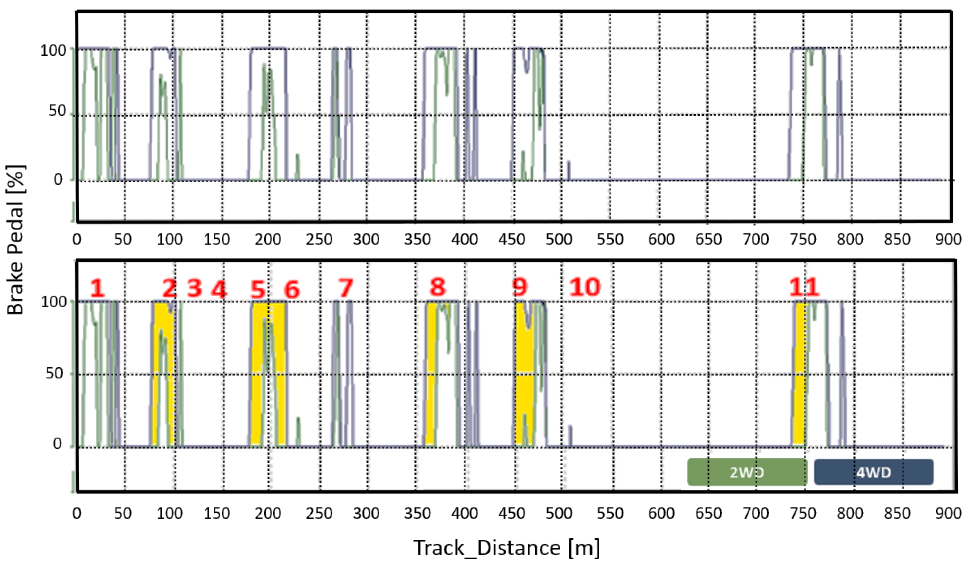
The analysis of the brake pedal actuation parameter is required to understand if the car is correctly balanced. The vehicle’s balance during braking improves as the brake pedal actuation becomes more aggressive. In regular vehicle braking, the brake pressure figure presents a progressive behavior. On the other hand, the behavior in racing vehicles must be as aggressive as possible, as the activation profile must be as close to 90° and the pressure removal must be instantaneous. In
Figure 25 it is possible to see this type of behavior, especially in the 4WD model. Another important observation to be analyzed concerning the difference in the pedal profile is that in the 4WD version, the brake activation always happens in advance and has a longer duration. This more severe behavior is because they reached speeds are much higher in the 4WD version compared to 2WD, so there is a greater need to apply the brake pedal more aggressively. This behavior is highlighted in yellow in the lower
Figure 25, the 11 corners are represented in red, according to the racetrack map previously explained in
Figure 13.
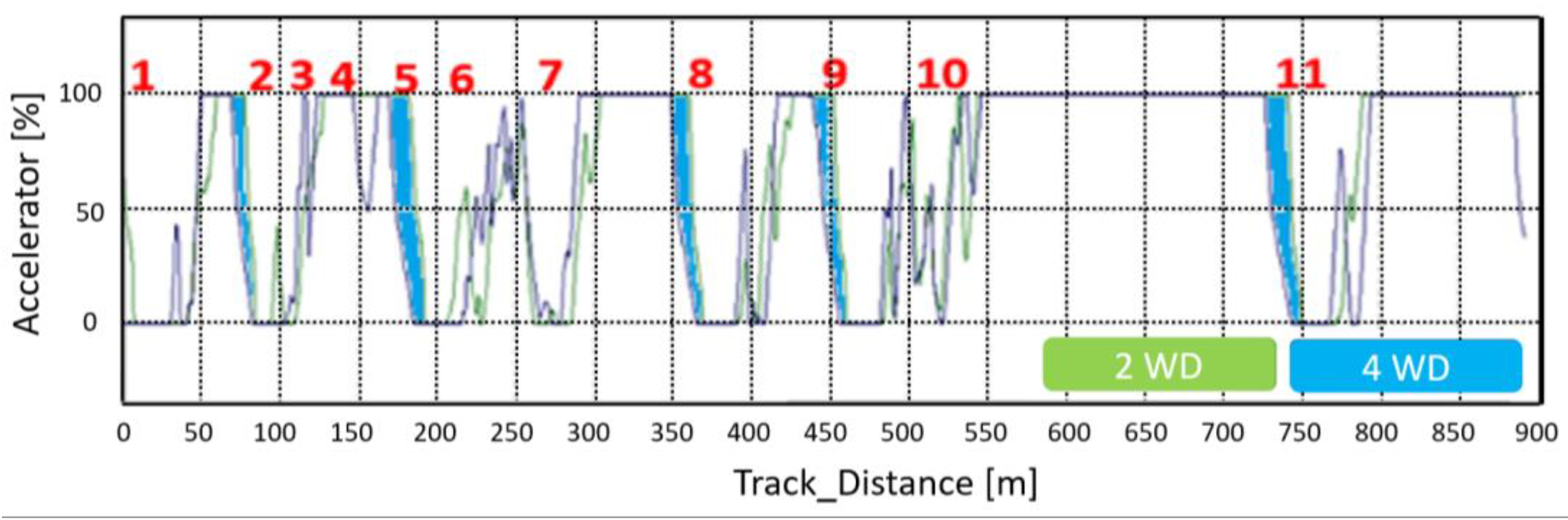
The last parameter analyzed is the accelerator pedal in
Figure 26. These data return the confidence level the racecar transmits to the driver when accelerating. For a racing vehicle, performance must stay at the top as long as possible with the throttle engaged at maximum level. This full-throttle drive indicates that the vehicle will be able to perform at high speed and, consequently, a faster lap time. The slight difference between curves is related to the speed and brake pedal actuation profiles, as analyzed above. As the 4WD vehicle arrives at the end of the straight at higher speeds than the 2WD vehicle, there is a need for the vehicle to start braking early. Moreover, the area highlighted in blue demonstrates these moments and the respective intensities.
5. Discussion
For the 2WD vehicle simulation modeling, different maneuvers were evaluated (Acceleration, Coastdown, Skidpad, and Autocross) to analyze the longitudinal and lateral dynamics separately. In summary, the velocity profile, acceleration values, engine rotation, deceleration, yaw rate, and steering wheel angle in the simulation and real test of a vehicle are similar. During the autocross maneuvers, the simulation showed a mere 0.6 s variance in lap completion time compared to the actual results. This suggests high accuracy in the simulation, especially considering the complexity of the vehicle and track model.
Using this 2WD vehicle simulation, it was possible to predict 4WD performance. Data indicate a slight difference in their lateral accelerations, meaning that both vehicles can traverse curves at similar speeds, whether the speeds are low or high. However, when it comes to reaching high speeds, the 4WD vehicle reaches the end of the straight faster than the 2WD vehicle [
36,
37,
38]. As a result, the 4WD vehicle must start braking earlier to compensate for its higher top speed. This resulted in a simulated lap time reduction of around 7.5%.
It is predicted that the 4WD car will exhibit higher speed due to the augmented traction force it possesses. However, as per the regulations of the competition, even with the motor and inverter combination being capable of delivering powers surpassing the 80 kW, the rules constrain the maximum power that can be used. This constraint is enforced by an energy meter, which monitors the energy consumption and peak levels of the car during all dynamic tests. Consequently, our car implements a strategy to control the maximum energy to be transferred (i.e., drawn) from the battery. As a result, the 4WD car will prevail in situations where the grip of the vehicle would be compromised, commonly referred to as oversteering or understeering (technically known as understeering and oversteering). Through torque vectoring, we can identify the wheel with the least traction on the road surface and reduce the energy transmitted to it. Conversely, the wheel with the greatest grip can receive a larger portion of the energy [
39].
6. Conclusions
The study of the 4WD technology with individual motors showed that one of the most significant advantages of using the four individual motors configuration is the precise torque distribution when applying the maximum motor power, allowing Torque Vectoring control. Furthermore, it improves the dynamic control stability, the driver’s confidence, and safety running in the most challenging types of race circuits or even grip levels. The simulation lap times performed by AVL VSM demonstrated this advantage. The 2WD vehicle performed the best lap time of 107.5% compared to the 4WD version. It means that the 2WD version is 3.5 s slower compared to the 4WD. In a race condition, with 22 laps, this difference would be around 75 s or 1.6 laps more for the 2WD version. Considering the track distance of around 900 m, the 4WD version would be capable of running an additional almost 1.5 km compared to 2WD. In formula SAE competition, as the drivers are non-professional, this technological advantage would be more beneficial than the top-level competitions with professional drivers. Another significant advantage of working with Torque Vectoring is the driver’s confidence due to the higher level of grip and car control stability, improving the driver’s lap times.
Although we already expected better performance from the 4WD car, we decided to assess and analyze the data from the 2WD car before constructing and testing the 4WD vehicle. This allowed us to gain insights and use simulation tools to predict the behavior and potential improvements of the 4WD configuration. Collecting accurate data from the 2WD car and utilizing simulation techniques to forecast the performance of the 4WD vehicle were crucial steps for us to plan and anticipate the potential benefits of the 4WD setup.
Author Contributions
Conceptualization, R.S.N.; Methodology, R.S.N. and M.R.; Software, R.S.N. and J.B.P.; Validation, R.S.N. and F.D.; Formal analysis, M.G.; Data curation, F.D.; Writing—original draft, R.S.N., G.B.R., M.G. and R.T.B.; Writing—review & editing, R.S.N., R.G., M.R., F.D., G.B.R., M.G. and R.T.B.; Supervision, R.G.; Project administration, R.G. and M.R.; Funding acquisition, R.S.N. and R.G. All authors have read and agreed to the published version of the manuscript.
Funding
This research was funded by the CNPq (National Research Council—Brazil) projects #436207/2018-4 and #306360/2020-9; FAPESP, Brazil #2017/18181-2, and #2018/25225-9—SPRACE; FINEP, Brazil Proc. #01.12.0224.00 and INCT-FNA, Brazil Proc. #464898/2014-5.
Data Availability Statement
Not applicable.
Conflicts of Interest
The authors declare no conflict of interest.
Appendix A. Control Strategy
Appendix A.1. Vertical Load Estimator
The control strategy considered the vertical load on each tire, according [
26], requiring the estimation of dynamic vertical loads. By multiplying the vehicle mass
by the longitudinal acceleration (
), we obtain the longitudinal force acting on the center of gravity (
), as presented in Equation (A1). This results in longitudinal load transfer. The longitudinal moment (
) can be calculated by Equation (A2) where is the center of gravity height (
).
By dividing the moment
by the wheelbase of the vehicle (
), we obtain the dynamic load transfer in the longitudinal direction (
) according to Equation (A3).
Next, we calculate the mass distributed between the front axle (
) and the rear axle (
), according to Equations (A4) and (A5), respectively.
The lateral slip of the vehicle (
) can be calculated from the relative velocities in the Y (
) and X (
) axes, as presented in Equation (A6).
The slip angles can be obtained by considering the yaw rate (
ψ′).
For the sake of analysis simplification, equal lateral friction coefficients will be adopted for both the front and rear axles. Thus, the lateral acceleration for the rear axle can be defined as
. The same calculation can be applied to the front axle, with the additional consideration of the steering angle.
The lateral friction coefficient is defined according to Equation (A11). Consequently, the lateral force on each axis can be defined as:
With the lateral forces of both axes calculated, it is possible to determine the relative lateral acceleration
that the vehicle is experiencing, and subsequently the yaw acceleration
ψ″.
To determine the yaw rate, we can integrate the yaw acceleration. The lateral acceleration can be expressed as follows:
Using the same method, we can estimate the lateral dynamic weight transfer
as well. Therefore, by considering the sum of longitudinal dynamic weight transfers
long and lateral dynamic weight transfers
, along with the static vertical load
, it is possible to estimate the load on each tire.
Maximum Lateral Acceleration Estimator
To calculate the maximum lateral acceleration, we can utilize the front and rear coefficients of lateral friction. By summing up all these lateral forces, we obtain the estimated maximum lateral acceleration.
Appendix A.2. Potencial
The tire potential (
) can be determined by Equation (A22), which considers the dynamic vertical load (
) and the lateral tire friction coefficient (
).
Appendix A.3. Lateral Saturation
By dividing the lateral force on each axis (
) by the potential lateral force (
), we obtain the saturation of each axis (
) as shown in Equation (A23). By definition, lateral saturation is the percentage of available lateral force, comparing the potential value that can be extracted from the mathematical tire model mentioned in this work with the lateral force at the moment the vehicle is in. Using this parameter ensures that the controller does not use unnecessary force energy to achieve the vehicle’s dynamic equilibrium, thus utilizing the necessary energy to achieve 100% of Lateral Saturation.
Appendix A.4. Controller Operation
To define the condition in which the controller is operating, we have the stability condition related to the condition in which the pilot finds themselves at the moment, for example, whether the condition is neutral, oversteering, or understeering. With that, it is possible to define the steer Gradient (
Ks), according to Equation (A25). The lower or higher Yaw Rate directly affects the
Ks condition, thus it should be the control parameter to determine how the Yaw Moment Control strategy should be applied.
Ks = 0, the vehicle is neutral;
Ks > 0, the vehicle is oversteering;
Ks < 0, the vehicle is understeering.
Appendix A.5. Lateral Slip
The stability control requires the implementation of a lateral slip estimator to complement the mass modeling strategy. Lateral slip poses a measurement challenge, requiring costly equipment and high implementation resources. Typically, laser sensors are used for measurement, but a strategy of estimators is employed to reduce cost and system complexity. These estimators are fixed parameters that enable the system to function effectively while minimizing costs and complexity.
References
- Requia, W.J.; Mohamed, M.; Higgins, C.D.; Arain, A.; Ferguson, M. How clean are electric vehicles? Evidence based review of the effects of electric mobility on air pollutants, greenhouse gas emissions and human health. Atmos. Environ. 2018, 185, 64–77. [Google Scholar] [CrossRef]
- Denton, T. Electric and Hybrid Vehicles, 1st ed.; Routledge: New York, NY, USA, 2016. [Google Scholar]
- Tong, W. Mechanical Design of Electric Motors, 1st ed.; CRC Press: New York, NY, USA, 2014. [Google Scholar]
- Ehsani, M.; Gao, Y.; Emadi, A. Modern Electric, Hybrid Electric, and Fuel Cell Vehicles: Fundamentals, Theory, and Design, 2nd ed.; CRC Press: Boca Raton, FL, USA, 2010. [Google Scholar]
- Alaee, P.; Bems, J.; Anvari-Moghaddam, A. A Review of the Latest Trends in Technical and Economic Aspects of EV Charging Management. Energies 2023, 16, 3669. [Google Scholar] [CrossRef]
- Kong, Z.; Zhang, W.; Zhang, H. Testing and Evaluation of the Electric Drive System on the Vehicle Level. World Electr. Veh. J. 2021, 12, 182. [Google Scholar] [CrossRef]
- Badin, F.; Le Berr, F.; Briki, H.; Dabadie, J.-C.; Petit, M.; Magand, S.; Condemine, E. Evaluation of EVs energy consumption influencing factors, driving conditions, auxiliaries use, driver’s aggressiveness. World Electr. Veh. J. 2013, 6, 112–123. [Google Scholar] [CrossRef] [Green Version]
- Zhou, Z.; Zhang, J.; Yin, X. Adaptive Sliding Mode Control for Yaw Stability of Four-Wheel Independent-Drive EV Based on the Phase Plane. World Electr. Veh. J. 2023, 14, 116. [Google Scholar] [CrossRef]
- Adeleke, P.; Li, Y.; Chen, Q.; Zhou, W.; Xu, X.; Cui, X. Torque Distribution Based on Dynamic Programming Algorithm for Four In-Wheel Motor Drive Electric Vehicle Considering Energy Efficiency Optimization. World Electr. Veh. J. 2022, 13, 181. [Google Scholar] [CrossRef]
- Rinderknecht, S.; Meier, T. Electric power train configurations and their transmission systems. In Proceedings of the SPEEDAM 2010—International Symposium on Power Electronics, Electrical Drives, Automation and Motion, Pisa, Italy, 14–16 June 2010; pp. 1564–1568. [Google Scholar]
- Pedret, P. Control Systems for High Performance Electric Cars. World Electr. Veh. J. 2013, 6, 88–94. [Google Scholar] [CrossRef] [Green Version]
- Feiqiang, L.; Jun, W.; Zhaodu, L. Motor Torque Based Vehicle Stability Control for Four-wheel-drive Electric Vehicle. In Proceedings of the Vehicle Power and Propulsion Conference 2009 VPPC 09, Dearborn, MI, USA, 7–11 September 2009; pp. 1596–1601. [Google Scholar]
- Cheli, F.; Melzi, S.; Sabbioni, E.; Vignati, M. Torque vectoring control of a four independent wheel drive electric vehicle. In Proceedings of the International Design Engineering Technical Conferences and Computers and Information in Engineering Conference, Portland, OR, USA, 4–7 August 2013. [Google Scholar]
- Jäger, B.; Neugebauer, P.; Kriesten, R.; Parspour, N.; Gutenkunst, C. Torque-vectoring stability control of a four-wheel drive electric vehicle. In Proceedings of the IEEE Intelligent Vehicles Symposium (IV), Seoul, Republic of Korea, 28 June–1 July 2015. [Google Scholar]
- Götting, G.; Kretschmer, M. Development and Series Application of a Vehicle Drivetrain Observer Used in Hybrid and Electric Vehicles. World Electr. Veh. J. 2013, 6, 364–372. [Google Scholar] [CrossRef] [Green Version]
- Gudey, S.K.; Malla, M.; Jasthi, K.; Gampa, K.R. Direct Torque Control of an Induction Motor Using Fractional-Order Sliding Mode Control Technique for Quick Response and Reduced Torque Ripple. World Electr. Veh. J. 2023, 14, 137. [Google Scholar] [CrossRef]
- Elamri, O.; Oukassi, A.; El Bahir, L.; El Idrissi, Z. Combined Vector and Direct Controls Based on Five-Level Inverter for High Performance of IM Drive. World Electr. Veh. J. 2022, 13, 17. [Google Scholar] [CrossRef]
- De Novellis, L.; Sorniotti, A.; Gruber, P.; Pennycott, A. Comparison of feedback control techniques for torque-vectoring control of fully electric vehicles. IEEE Trans. Veh. Technol. 2014, 63, 3612–3623. [Google Scholar] [CrossRef]
- Liebemann, E.K.; Meder, K.; Schuh, J.; Nenninger, G. Safety and Performance Enhancement: The Bosch Electronic Stability Control (ESP). In Proceedings of the Fourth International Conference on Modeling, Simulation and Applied Optimization, Kuala Lumpur, Malaysia, 19–21 April 2014. [Google Scholar]
- Mikle, D.; Bat, M. Torque Vectoring for an Electric All-wheel Drive Vehicle; IFAC (International Federation of Automatic Control) Hosting by Elsevier Ltd.: Luxembourg, 2019; pp. 163–169. [Google Scholar]
- Tahouni, A.; Mirzaei, M.; Najjari, B. Novel Constrained Nonlinear Control of Vehicle Dynamics Using Integrated Active Torque Vectoring and Electronic Stability Control. IEEE Trans. Veh. Technol. 2019, 68, 9564–9572. [Google Scholar] [CrossRef]
- Li, Y.; Ren, J.; Yang, Q. Predictive Control of Surface PMSM Direct Torque Control System using Voltage Vectors with Variable Angle. In Proceedings of the IEEE Student Conference on Electric Machines and Systems, Huzhou, China, 14–16 December 2018. [Google Scholar]
- Amornwongpeeti, S.; Kiselychnyk, O.; Wang, J.; Shatti, N.; Shah, N.; Soumelidis, M. Adaptive torque control of IPMSM motor drives for electric vehicles. In Proceedings of the IEEE 26th International Symposium on Industrial Electronics (ISIE), Edinburgh, UK, 19–21 June 2017. [Google Scholar]
- Formula SAE International Rules. Available online: https://www.fsaeonline.com/cdsweb/gen/DocumentResources.aspx (accessed on 17 January 2022).
- AVL VSM 4™. Available online: https://www.avl.com/en (accessed on 21 March 2021).
- Milliken, W.; Milliken, D. Race Car Vehicle Dynamics; SAE International: Warrendale, PA, USA, 1994. [Google Scholar]
- ISO 10521-1:2006; Road Vehicles—Road Load—Part 1: Determination under Reference Atmospheric Conditions. ISO: Geneva, Switzerland, 2006.
- Simcenter STAR-CCM+ Software. Available online: https://plm.sw.siemens.com (accessed on 9 May 2022).
- Sugano, T.; Fukuba, H.; Suetomi, T. A study of dynamics performance improvement by rear right and left independent drive system. Veh. Syst. Dyn. 2010, 48, 1285–1303. [Google Scholar] [CrossRef]
- Medina, A.; Bistue, G.; Rubio, A. Comparison of Typical Controllers for Direct Yaw Moment Control Applied on an Electric Race Car. Vehicles 2021, 3, 127–144. [Google Scholar] [CrossRef]
- Yin, G.; Wang, R.; Wang, J. Robust control for four wheel independently-actuated electric ground vehicles by external yaw-moment generation. Int. J. Automot. Technol. 2015, 16, 839–847. [Google Scholar] [CrossRef]
- Zhang, C.; Ma, J.; Chang, B.; Wang, J. Research on Anti-Skid Control Strategy for Four-Wheel Independent Drive Electric Vehicle. World Electr. Veh. J. 2021, 12, 150. [Google Scholar] [CrossRef]
- Ci, L.; Zhou, Y.; Yin, D. An Anti-Skid Control System Based on the Energy Method for Decentralized Electric Vehicles. World Electr. Veh. J. 2023, 14, 49. [Google Scholar] [CrossRef]
- Shuai, Z.; Zhang, H.; Wang, J.; Li, J.; Ouyang, M. Lateral motion control for four-wheel-independent-drive electric vehicles using optimal torque allocation and dynamic message priority scheduling. Control Eng. Pract. 2014, 24, 55–66. [Google Scholar] [CrossRef]
- Alipour, H.; Sabahi, M.; Sharifian, M.B.B. Lateral stabilization of a four wheel independent drive electric vehicle on slippery roads. Mechatronics 2015, 30, 275–285. [Google Scholar] [CrossRef]
- De Pinto, S.; Camocardi, P.; Chatzikomis, C.; Sorniotti, A.; Bottiglione, F.; Mantriota, G.; Perlo, P. On the Comparison of 2- and 4-Wheel-Drive Electric Vehicle Layouts with Central Motors and Single- and 2-Speed Transmission Systems. Energies 2020, 13, 3328. [Google Scholar] [CrossRef]
- Varela, A.B.; Irlinger, F. A Feasibility Study on Driver Model Based Lap Time Simulation Using Genetic Algorithms. SAE Int. J. Passeng. Cars Mech. Syst. 2017, 10, 401–412. [Google Scholar] [CrossRef]
- Ghosh, J.; Tonoli, A.; Amati, N. Improvement of Lap-time of a Rear Wheel Drive Electric Racing Vehicle by a Novel Motor Torque Control Strategy. In Proceedings of the SAE World Congress Experience 2017, Detroit, MI, USA, 4–6 April 2017. [Google Scholar]
- Kobayashi, I.; Ogawa, K.; Uchino, D.; Ikeda, K.; Kato, T.; Endo, A.; Peeie, M.H.B.; Narita, T.; Kato, H. A Basic Study on Hybrid Systems for Small Race Car to Improve Dynamic Performance Using Lap Time Simulation. Actuators 2022, 11, 173. [Google Scholar] [CrossRef]
Figure 1.
Formula FEI TV vehicle.
Figure 1.
Formula FEI TV vehicle.
Figure 2.
Main vehicle parameter data utilized as input for the simulator.
Figure 2.
Main vehicle parameter data utilized as input for the simulator.
Figure 3.
Indication of the sensor’s location.
Figure 3.
Indication of the sensor’s location.
Figure 4.
Image from (a) Tire temperature sensors (b) brake disc temperature sensor and (c) suspension displacement sensor.
Figure 4.
Image from (a) Tire temperature sensors (b) brake disc temperature sensor and (c) suspension displacement sensor.
Figure 5.
AVL VSM software, input parameters from tire system model.
Figure 5.
AVL VSM software, input parameters from tire system model.
Figure 6.
AVL VSM software indicating the Kinematics Compliance parameters.
Figure 6.
AVL VSM software indicating the Kinematics Compliance parameters.
Figure 7.
Chassis torsional stiffness measurement optical photometry to be imputed on VSM™.
Figure 7.
Chassis torsional stiffness measurement optical photometry to be imputed on VSM™.
Figure 8.
On the (left) the brake pad test in the dynamometer to extract the friction coefficient of the breaks. On the (right) the visual operating range temperatures.
Figure 8.
On the (left) the brake pad test in the dynamometer to extract the friction coefficient of the breaks. On the (right) the visual operating range temperatures.
Figure 9.
AVL VSM software indicating powertrain parameters.
Figure 9.
AVL VSM software indicating powertrain parameters.
Figure 10.
CFD analysis from Formula FEI TV vehicle.
Figure 10.
CFD analysis from Formula FEI TV vehicle.
Figure 11.
ECPA circuit for acceleration and Coastdown maneuver.
Figure 11.
ECPA circuit for acceleration and Coastdown maneuver.
Figure 12.
Formula SAE skid-pad test geometry [
24].
Figure 12.
Formula SAE skid-pad test geometry [
24].
Figure 13.
Interlagos circuit, in which the vehicle traveled around the Autocross.
Figure 13.
Interlagos circuit, in which the vehicle traveled around the Autocross.
Figure 14.
Example of a racetrack captured by the AVL program.
Figure 14.
Example of a racetrack captured by the AVL program.
Figure 15.
Simulation and experimental comparison acceleration maneuver.
Figure 15.
Simulation and experimental comparison acceleration maneuver.
Figure 16.
Coastdown test results.
Figure 16.
Coastdown test results.
Figure 17.
Simulation and test comparison for Skidpad maneuver.
Figure 17.
Simulation and test comparison for Skidpad maneuver.
Figure 18.
Lateral acceleration diagram as a function of steering wheel angle.
Figure 18.
Lateral acceleration diagram as a function of steering wheel angle.
Figure 19.
Simulation and testing comparison in an Autocross lap.
Figure 19.
Simulation and testing comparison in an Autocross lap.
Figure 20.
Autocross lap time sensitivity study.
Figure 20.
Autocross lap time sensitivity study.
Figure 21.
Two-wheel drive and four-wheel drive vehicle.
Figure 21.
Two-wheel drive and four-wheel drive vehicle.
Figure 22.
Comparison of 4WD vs. 2WD on Autocross lap time.
Figure 22.
Comparison of 4WD vs. 2WD on Autocross lap time.
Figure 23.
Speed gains due to increased traction capacity of the 4WD vehicle.
Figure 23.
Speed gains due to increased traction capacity of the 4WD vehicle.
Figure 24.
Comparison of steering angle during the Autocross lap.
Figure 24.
Comparison of steering angle during the Autocross lap.
Figure 25.
Brakes activation comparison during the Autocross lap.
Figure 25.
Brakes activation comparison during the Autocross lap.
Figure 26.
Comparison of accelerator activation during the Autocross lap.
Figure 26.
Comparison of accelerator activation during the Autocross lap.
Table 1.
Sensor’s models.
Table 1.
Sensor’s models.
| Sensor | Model | Manufacturer |
|---|
| Tire temperature | INFKL 200 °C | Texense (Nevers, France) |
| Wheel speed | RS-M10WS | Texense (Nevers, France) |
| Brake temperature | INFLK 800 °C | Texense (Nevers, France) |
| LVDT | RSL position transducer | Texense (Nevers, France) |
| Accelerometers | AC-CAP 3 axis | Texense (Nevers, France) |
| Gyros | GYRN-S 3 axis | Texense (Nevers, France) |
| Brake pressure | EPT 3100 | Texense (Nevers, France) |
| TPS e BPSRotary Sensor | SP2800 | Novotechnik Inc. (Southborough, MA, USA) |
| Cooling | TS-NTC Fluid Temperature Sensor | Texense (Nevers, France) |
| HV battery current sensor | G1 BMS | EMUS UAB (Vilnius, Lithuania) |
| Steering angle | RSL position transducer | Texense (Nevers, France) |
| Disclaimer/Publisher’s Note: The statements, opinions and data contained in all publications are solely those of the individual author(s) and contributor(s) and not of MDPI and/or the editor(s). MDPI and/or the editor(s) disclaim responsibility for any injury to people or property resulting from any ideas, methods, instructions or products referred to in the content. |
© 2023 by the authors. Licensee MDPI, Basel, Switzerland. This article is an open access article distributed under the terms and conditions of the Creative Commons Attribution (CC BY) license (https://creativecommons.org/licenses/by/4.0/).


 ,
, 


