Article

Adaptive Sliding Mode Control for Yaw Stability of Four-Wheel Independent-Drive EV Based on the Phase Plane

1
College of Vehicle and Traffic Engineering, Henan University of Science and Technology, Luoyang 471003, China
2
Ningbo Shenglong Group Co., Ltd., Ningbo 315104, China
*
Author to whom correspondence should be addressed.
World Electr. Veh. J. 2023, 14(5), 116; https://doi.org/10.3390/wevj14050116
Submission received: 5 March 2023 / Revised: 18 April 2023 / Accepted: 19 April 2023 / Published: 23 April 2023

Abstract

:
Aiming at the yaw stability problem of a four-wheel independent-drive electric vehicle (EV) during steering, this paper proposes an adaptive sliding mode control strategy (ASMC) for yaw stability based on the phase plane. The control strategy adopts hierarchical control. The upper layer is the ASMC controllers based on particle swarm optimization (PSO). Aiming at the chattering problem of sliding mode controller, the approach law is designed as the adaptive approach law, which changes with the change of system state by using the adaptive control principle; to minimize the response delay and tracking error, the control system is taken as the object to find a set of optimal parameters for a constant velocity approach rate based on PSO. The middle level is a joint controller, which uses the established β β ˙ phase plane stability region boundary model to control the upper-level controllers jointly. When the vehicle is in the stable region, the ASMC controller for the yaw rate is used to determine the yaw moment; when the vehicle is outside the stable region, the final yaw moment is determined by the ASMC controller for the yaw rate and the ASMC controller for the sideslip angle, to restore the stability of the vehicle. The lower layer is a torque optimal distribution controller, which converts the yaw moment into torque and optimally distributes it to four wheels. Finally, Simulink and CarSim platforms are used for joint simulation. The results prove that the proposed control strategy can effectively reduce the error between the actual and the ideal value of control parameters and improve the vehicle’s stability when steering.

1. Introduction

When the four-wheel independent-drive EV turns at high speed, it will produce a sizeable lateral acceleration and sideslip angle, leading to serious traffic accidents such as a sideslip or rollover, and seriously affect the vehicle’s handling stability. Therefore, we need to exert some control on the vehicle during steering to improve the vehicle’s handling stability and ensure the driver’s safety [1,2,3].
Some studies have shown that yaw moment control can improve the vehicle’s handling stability [4,5]. The sliding mode control (SMC) is widely used in automotive engineering because of its robustness and simplicity [6,7]. In recent years, more and more researchers have applied SMC to stability control and achieved a certain degree of success [8,9]. Wang YC et al. proposed a prediction controller to obtain the anticipant yaw moment [10]. Zhang H Z et al. proposed a fuzzy SMC(FSMC) strategy to improve the controller’s input smoothness and to obtain the yaw moment [11]. Mousavi E et al., based on SMC theory, established a yaw stability controller but ignored the error change rate of the variables and reduced the controller’s accuracy [12]. Although Bagheri et al. took the error change of control variables into account, they did not analyze the torque distributor. The average torque distribution method is hard to adapt to complex working conditions and has certain limitations [13]. In addition, Zhou H et al. pointed out the shortcomings of the SMC method in the control principle. They considered that the chattering problem severely impacted the controller’s stability [14]. Wang et al. used an exponential approach rate to design a sliding mode control rate to suppress system chattering [15]. Le et al. used the saturation function to supersede the symbolic function to ensure the continuity of the input, maintain the accuracy and suppress the chattering of the system [16]. Wang H et al. adopt the integral SMC method to obtain the desired yaw moment by controlling both the yaw rate and the sideslip angle [17]. Zhang F proposed a nonlinear controller based on SMC and Lyapunov theory to obtain the ideal additional yaw moment of the vehicle to keep the vehicle stable [18]. Zhu H proposed an improved adaptive nonsingular fast terminal SMC to improve the stability of the electric bus [19].
In addition, some scholars use the phase plane to study vehicle stability. Farroni F. et al. use the phase plane to study the influence of tire nonlinearity on vehicle handling, and an integrated active steering controller is designed to enhance vehicle stability under extreme conditions [20]. Vignati M. et al. proposed that the torque vector distribution helps accelerate the yaw rate convergence to the phase plane balance point [21]. Cui Y et al. propose an active steering integrated controller, mainly used for vehicles running under extreme conditions to ensure stable driving [22]. Zhu S. uses the phase plane law to divide the phase plane stability region of the vehicle and introduces the stability quantification index PPS-region for the evaluation of vehicle stability [23]. Based on the phase plane, Zhong F. L. designed a partition controller, which uses a fuzzy neural network and PID controller to jointly decide the yaw moment when the vehicle is unstable to restore the vehicle to stability. However, the coupling between control variables is ignored in the control process [24]. Based on the optimized phase plane method, Zhou B. divided the stable regions and adopted different control methods in different regions to achieve joint control of active front wheel steering (AFS) and direct yaw moment control (DYC) [25]. Liu X. C. et al. designed a stability controller in the unstable region based on the two-phase planes of yaw rate and sideslip angle. However, they did not involve the control of the vehicle in the stable region [26]. Therefore, we need to do further research.
The above research mainly uses different control methods to improve the vehicle’s yaw stability. However, there are still some issues to consider with the current study. On the one hand, for the design of the SMC controller, most studies have designed the sliding mode reaching law using different methods. However, most sliding mode reaching rates are fixed values, which is challenging to meet the system’s reaching speed and chattering suppression. On the other hand, there are few types of research on the coupling between control variables. For example, the yaw rate and the sideslip angle are the main control parameters. Because of their coupling, we need to control them to improve the vehicle handling stability jointly.
Aiming at the above problems, an ASMC for yaw stability based on β β ˙ phase plane is proposed. The control strategy adopts hierarchical control. The upper layer is the ASMC controllers based on PSO optimization. The middle level is a joint controller based on the established β β ˙ phase plane stability region boundary model, and according to the different states of the vehicle, different control methods are used to control the vehicle. When the vehicle is in the stable region, the ASMC controller for the yaw rate is used to determine the yaw moment; when the vehicle is outside the stable region, the yaw moment is determined by the ASMC controller for the yaw rate and the ASMC controller for the sideslip angle. The lower layer is a torque optimal distribution controller, which converts the yaw moment into torque and optimally distributes it to four wheels. Finally, Simulink and CarSim platforms are used for joint simulation. The consequences attest that the controller can effectively reduce the error between the ideal and the actual values of the control variables, the maximum error of the yaw rate did not exceed 0.012 rad/s, the maximum error of the sideslip angle did not exceed 0.02 rad and enhanced the stability of the vehicle when steering.
The remainder of this article is organized as follows.
In Section 2, the dynamic model is established. In Section 3, the β β ˙ phase plane is established. In Section 4, the stability controller of a vehicle is established. In Section 5, the simulation experiment results are discussed. In Section 6, the conclusion is provided.
Main contributions of this paper.
Compared with the above research, the research in this paper is different and novel in the following two aspects.
(1) On the one hand, we use the adaptive control principle and PSO to improve the sliding mode controller, to more effectively suppress the chattering problem of the system, and further improve the working efficiency of the controller;
(2) On the other hand, through the established β β ˙ phase plane stability region boundary model to jointly control the upper-level controllers. The established phase plane is divided into three regions: stable control region, coordinated control region and unstable control region. According to the different states of the vehicle, different control methods are used to control the vehicle. Through the above control strategy, we can solve the coupling problem before the yaw rate and the sideslip angle to better play the effect of the yaw moment controller.

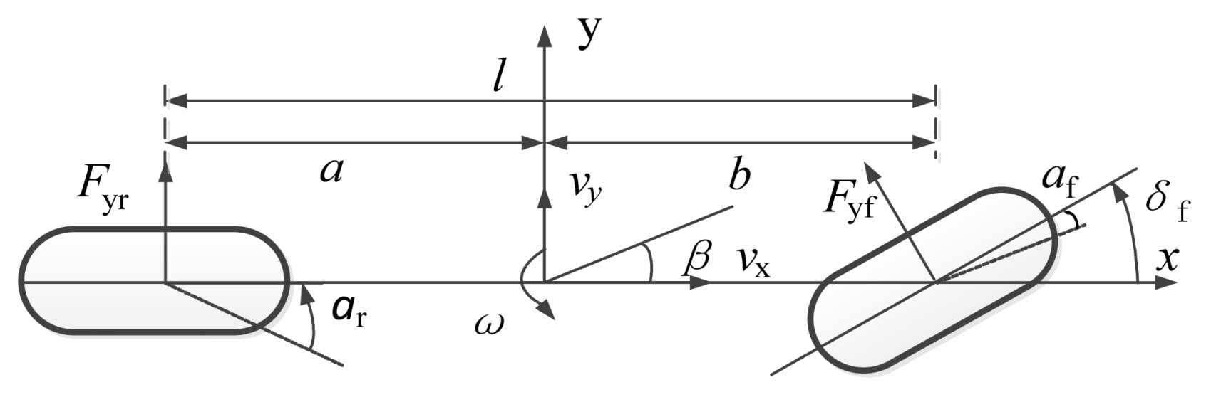
2. Vehicle Dynamic Model

2.1. Reference Model

The 2-DOFs vehicle model can obtain the value of the yaw rate and the sideslip angle when the vehicle is turning [27], as shown in Figure 1.
The differential equation is defined as
{ β ˙ = k f + k r m v x β + ( a k f b k r m v x 2 1 ) ω k f m v x δ f ω ˙ = a k f b k r I z β + a 2 k f + b 2 k r I z v x ω a k f I z δ f
where ω is the yaw rate; β is the sideslip angle; K f and K r are the front and rear axle cornering stiffness; δ f is the front wheel angle; I z is the moment of inertia of the vehicle about the z-axis; m is the vehicle mass; v x is the longitudinal velocity.
The constraints are expressed as
{ | ω max | = μ g v x | β max | = μ g ( b v x 2 + m a k r L )
where μ is the road adhesion coefficient; L is the wheelbase.
When the β ˙ = 0 , ω ˙ = 0 , we can obtain the ideal value:
{ ω d = min { | v x L ( 1 + K v x 2 ) δ | , | ω max | } sgn ( δ ) β d = min { | b L + m a v x 2 / ( k r L 2 ) 1 + K v x 2 δ f | , | μ g ( b v x 2 + m a k r L ) | } sgn ( δ f )

2.2. Tire Model

The tire model adopts the magic tire formula with high fitting accuracy and easy use. This model has the advantages of fewer parameters, and one formula can fully express the longitudinal force, lateral force, and return moment of the tire. The expression is defined as [28]
Y ( x ) = D sin { C arctan [ B x E arctan ( B x ) ] } + S v
where Y is the longitudinal force; D is the peak factor; B is the stiffness factor; C is the curve shape factor; S v is vertical drift; X is the longitudinal slip rate; E is the curvature factor.
When the vehicle is running, the vertical load of the tire will change with the axle load transfer. However, on the premise that the ground adhesion condition remains unchanged, increasing the vertical tire load will increase the tire lateral force, so the relationship between the parameters and the vertical load F Z needs to be considered in control.
{ B = B C D / ( C D ) C = a 0 D = ( a 1 F z 2 + a 2 F z ) B C D = a 3 sin ( 2 a t c tan F z a 4 ) × ( 1 a 5 | ξ | ) E = ( a 6 F z + a 7 ) S h = a 8 ξ + a 9 F z + a 10 S v = a 11 F z ξ + a 12 F z + a 13 X 1 = ( α + S h )
where ai (i = 0, 1, …,13) is the fitting coefficient; ξ is the wheel camber; α is the wheel sideslip angle; S h is the horizontal offset; F z is the wheel vertical load.
Calculation of vertical load
{ F z f = ( m g b ) / L F z r = ( m g a ) / L
where F z f and F z r are the vertical load distance between the front and rear wheels.
Calculation of sideslip angle
{ α f = β + a γ / v x δ α r = β b γ / v x
where α f and α r are the sideslip angle between the front and rear wheels.

3. Establishment of Phase Plane
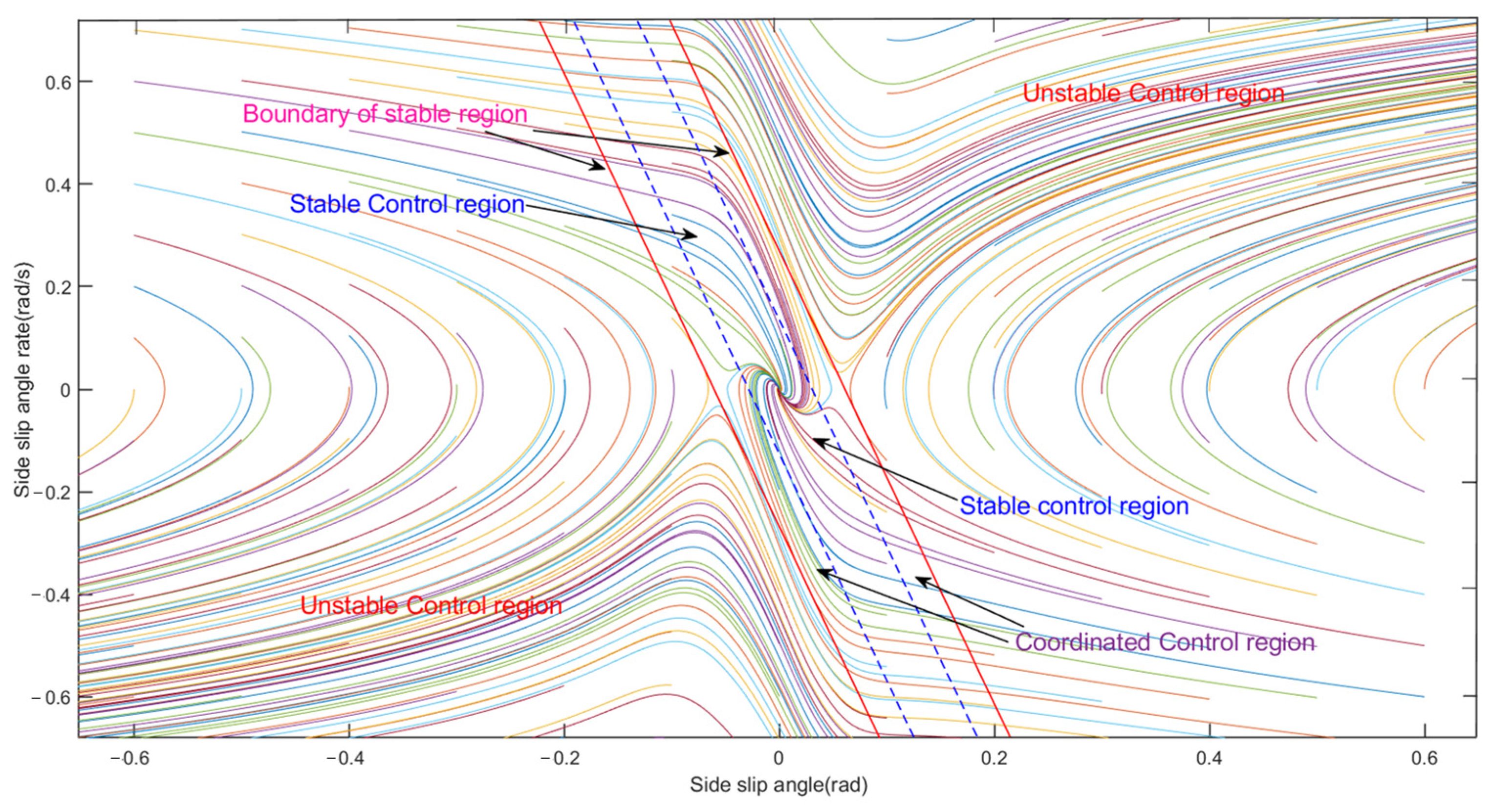
When the vehicle is in an unstable state, the β γ phase plane is prone to miscalculation and the β β ˙ phase plane is more accurate [29]. Therefore, in this paper, the β β ˙ phase plane is established as the criterion for vehicle instability.

3.1. Establishment of β β ˙ Phase Plane and Division of Stability Region

According to the 2-DOF model established, the sideslip angle and yaw rate are taken as the variables, and the second-order system is expressed as
{ β ˙ = f 1 ( β , γ ) γ ˙ = f 2 ( β , γ )
According to Formula (8), the β β ˙ phase plane established is shown in Figure 2.
For the division of the stability region, two parallel lines symmetrical about the origin are usually used to divide the phase trajectory into the stability region and the instability region. The region surrounded by two boundary lines is the stability region. As shown in Figure 2, the boundary equation is
| β ˙ + k β | c
where k is the slope of the boundary line; c is the intercept of boundary line; the values of k an c are related to the factors affecting the phase plane.

3.2. Stable Boundary Equation of β β ˙ Phase Plane

In practical application, the influence of the front wheel angle on the stability boundary of the β β ˙ phase plane can be ignored [30], so this paper only considers the influence of μ .
The boundary parameters k and c under different values of μ as shown in Table 1.
According to Table 1, with the increase in μ , the intercept of the stable boundary c increases, and the slope k decreases. Therefore, the stability region increases with the increase in μ , which is in line with the actual situation.
The boundary equation is
{ | β ˙ + k β | c k = 0.783 μ 2 3.793 μ 0.632 c = 0.079 μ 2 0.147 μ + 0.033

4. Design of Yaw Stability Controller

The controller based on β β ˙ phase plane design includes upper, middle and lower layers. The upper layer is ASMC controllers, which outputs the additional yaw moment, respectively. The middle layer is a joint controller, which judges the stability of the vehicle according to the β β ˙ phase plane to balance the scope of the two controllers. The lower controller calculates the final moment and distributes the optimized torque to the wheels; the specific structure is shown in Figure 3.

4.1. Design of ASMC Controller for Yaw Rate

Because the sliding mode surface and sliding mode motion characteristics are designed in advance, the system is insensitive to external interference, has strong robustness and the algorithm is simple.
The differential equation of the 2-DOFs model of Formula (1) is rewritten as
{ β ˙ = k f + k r m v x β + ( a k f b k r m v x 2 1 ) ω k f m v x δ ω ˙ = a k f b k r I z β + a 2 k f + b 2 k r I z V x ω a k f I z δ + M i I z
where M i is the additional yaw moment, the value of i is related to the control variable. When the control variable is yaw rate, i = ω ; when the control variable is the sideslip angle, i = ω .
To ensure the wheels are in the ideal linear range, the sliding surface is defined as
S ω = c ω e ω + e ˙ ω .
Derived from S ω
S ˙ ω = c ω e ˙ ω + e ¨ ω
where e ω is the error between the ideal and the actual value of the control variable; c ω is the relative weight coefficient.
A sliding mode approach law with exponential approach characteristics is selected to suppress the chattering.
S ˙ ω = K ω sgn ( S ω ) ε ω S ω
where K ω and ε ω are constants, and K ω > 0 , ε ω > 0 .
If K ω is a fixed value, the controller we have established will not be able to ensure a fast-reaching law while suppressing system chattering. Therefore, in order to solve the above problem, we design K ω as an adaptive parameter K ω 0 that changes with system state changes.
{ S ˙ ω 0 = K ω 0 sgn ( S ω ) ε ω S ω K ω 0 = h γ + ( 1 + 1 | e ω | γ ) e τ · | S ω |
where parameters h > 0 ; τ > 0 ; 0 < γ < 1 .
If the system state is far away from the sliding mode surface, | S ω | , K ω 0 tends to the constant h y , ( h y > h ), so the approaching speed is increasing; if the system state approaches the sliding mode surface, | S ω | 0 , K ω 0 tends to h | e ω | 1 + | e ω | , and with the decrease in e ω , the approach rate gradually approaches 0, thus effectively reducing the system chattering.
By introducing Formulas (3) and (11) into Formula (12), it can be obtained that
s ˙ ω = c ω e ˙ ω + e ¨ ω = c ω e ˙ ω + ω ¨ ω ¨ d = c ω e ˙ ω + a k f b k r I z β ˙ + a 2 k f + b 2 k r I z δ ˙ + M ω I z ω ¨ d
In order to have good quality during the movement of the system to the sliding surface, it is determined that the calculation formula for the additional yaw moment is
M ω = I z ( c ω e ˙ ω + a k f b k r I z β ˙ a 2 k f + b 2 k r I z V x ω ˙ a k f I z δ ˙ ω ¨ d + K ω 0 sgn ( S ω ) + ε ω S ω )
In order to further suppress the chattering of the system, replace the sign function in Formula (16) with the saturation function.
s a t ( s ω ) = { 1 , s ω > H k ω s ω , | s ω | H , k ω = 1 H 1 , s ω < H
where H is the boundary layer; k ω is a constant.

4.2. Design of ASMC Controller for Sideslip Angle

The sideslip angle is most sensitive to vehicle handling [31]. Therefore, a sliding surface is defined to prevent the actual sideslip angle from being too large.
S β = c β e β + e ˙ β
After taking the derivative of S β
S ˙ β = c β S ˙ β = c β e ˙ β + e ¨ β .
Concerning Formula (15), the approach mode of sliding mode is defined as
S ˙ β = K β 0 sgn ( S β ) ε β S β .
According to Formulas (19) and (11), the M β is defined as
M β = a k f ( δ f β ) + β b k r a 2 k f + b 2 k r v x ω z I z ( K β 0 s a t ( S β ) + ε β S β + c β e ˙ β + k f + k r m v x β ˙ k f m v x δ ˙ f β ¨ d ) / a k f b k r m v x 2 1

4.3. Stability Analysis of Control System

Take the yaw rate as an example to analyze the stability of the control system. Define the Lyapunov function as
L = s 2 2 .
It can be obtained after calculating the first derivative.
L ˙ = s ω s ˙ ω = s ω ( c ω e ˙ ω + a k f b k r I z β ˙ + a 2 k f + b 2 k r I z v x ω ˙ a k f I z δ ˙ + M ω I z ω ¨ d ) .
It can be obtained after M ω is brought in
L ˙ = s ω ( K ω 0 sgn ( s ω ) ) = { K ω 0 | s ω | , | s ω | > H K ω 0 k ω s ω 2 , | s ω | H
because K ω 0 > 0 and k ω > 0 , L ˙ 0 , the system is stable.

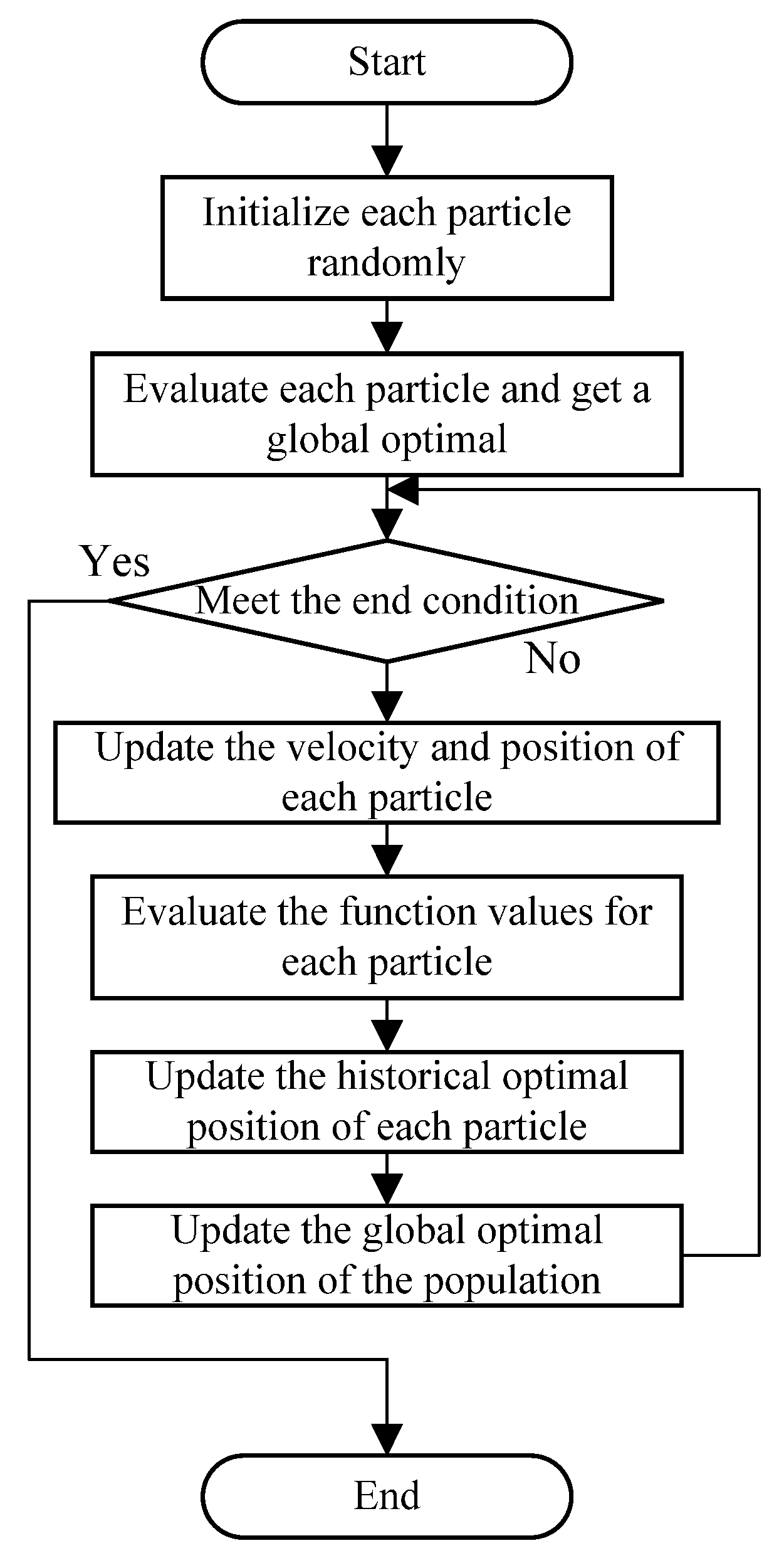
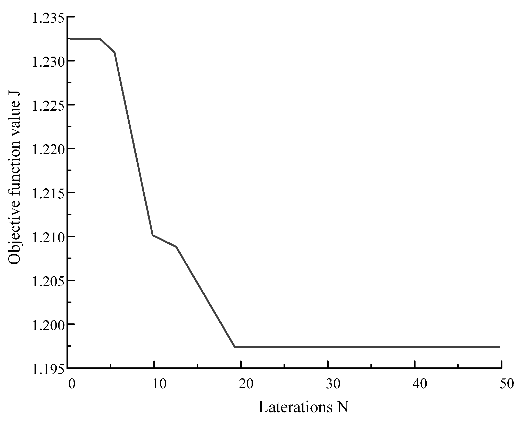
4.4. Particle Swarm Optimization of Sliding Mode Control Parameters

PSO is a process in which a group of designed random particles finds the optimal solution [32]. The calculation of velocity update mainly depends on the velocity value at the previous time, the difference between the current position and the optimal historical position of the particle swarm. The specific calculation formula is defined as
V i ( t + 1 ) = ω V i ( t ) + c 1 r 1 ( p b e s t i x i ( t ) ) + c 2 r 2 ( g b e s t x i ( t ) )
The position update only requires the last quarter’s position value and speed value. The calculation formula is defined as
x i ( t + 1 ) = x i ( t ) + v i
where V i ( t ) represents the velocity value of the ith particle at time t ; p b e s t i represents the historical optimal position of the ith particle; ω represents velocity inertia weight; g b e s t represents the historical optimal value of the entire particle swarm; c 1 is a self-learning factor; c 2 is the group learning factor; r 1 and r 2 is used to increase the randomness of the search. Figure 4 shows the control flow of particle swarm optimization algorithm.
To minimize the response delay and tracking error, the yaw rate control system is taken as the object to find a set of optimal parameters for constant velocity approach rate ε ω and sliding surface coefficient c ω .
Taking e ω and M ω as indicators, the objective function is defined as
J = 0 a | e ω ( t ) | + b | M ω ( t ) | d t
where a is the weight of tracking error and b is the weight of control quantity
MATLAB calculates the objective function value, and PSO is carried out to obtain the optimal parameter solution. However, due to the discrete and finiteness of the numerical calculation, which is contrary to the above objective function, the infinite integral of the objective function is changed into a finite summation during the actual experiment and calculation, and the modified objective function is as follows:
J = i = s t a r t i = e n d ( a | e ω ( i ) | T s t e p + b | M ω ( i ) | T s t e p )
where T s t e p is the simulation step and T s t e p = 0.001 s.
The evolution process curve is shown in Figure 5.
When the number of iterations N = 19, the optimal value J = 1.1975 can be obtained.
The optimized parameters are shown in Table 2.
Similarly, the optimized value of c β and ε β are shown in Table 3.

4.5. Joint Controller

The output value of the yaw rate controller is taken as the final yaw moment in the stability control region; two controllers jointly decide the final yaw moment in the coordinated control region; the output value of the sideslip angle controller is taken as the final yaw moment in the unstable control region. The division of the β β ˙ phase plane control domain is shown in Figure 6. In the figure, the two parallel red curves are the boundary lines of the stability region, and the two parallel blue dashed lines are the boundary lines of the joint control region.
When the value of μ decreases, the range of the phase plane stability zone becomes smaller, so the boundary condition of the joint control zone is
μ | 1 c β ˙ + k c β | 1
In the joint control domain, the ASMC controllers work together. The weight coefficient is quoted to balance the two controllers’ proportions. The formula of the total yaw moment is
M u = G M ω + ( 1 G ) M β
The relationship between the weight coefficient G and the stable boundary is shown in Figure 7.
The maximum yaw moment that the ground can provide as
M u max = d μ ( F x 2 + F x 4 F x 1 F x 3 ) / 2
where F x 1 , F x 2 , F x 3 and F x 4 are the longitudinal forces of the four wheels, respectively; d is the wheel track.
M u max and M u are compared, and the smaller value is output to the lower layer controller as the target yaw moment.
M z = min { M u , M u max }

4.6. Drive Torque Distribution

The yaw moment is converted into the torque of wheels through the lower controller, and the moment control during vehicle steering is realized through the vehicle dynamics model [33].
In this paper, the quadratic programming method is used to optimize the distribution of yaw moment, and the process is as follows:
The optimization objective function
min J = min i = 1 4 F x i 2 ( μ i F z i ) 2 = min i = 1 4 T x i 2 ( μ i F z i R ) 2 .
Considering the requirements of yaw moment and total drive torque, as well as the limitations of motor peak torque and road adhesion coefficient, the following constraints are established:
{ T x 1 + T x 2 + T x 3 + T x 4 = T t B f 2 R ( T x 2 T x 1 ) cos δ f + B r 2 R ( T x 4 T x 3 ) = M z T x i μ R F z i T x i T max
where T x i and F z i is the torque and the vertical load of wheels; T max is the maximum output torque.
Finally, using the Quadprog function in MATLAB to solve, the four tire torques are optimally distributed.

5. Simulation Analysis

In this paper, a driver model is built in Simulink for simulation, and different steering wheel angle inputs are provided based on the driver model built. In Section 5.1, we use the steering wheel angle sine input open-loop simulation mode and the double shift closed loop simulation mode to compare the ASMC controller designed in this article with ordinary SMC controllers and prove the effectiveness of the ASMC controller. In Section 5.2, we use a line change simulation experiment to compare the ASMC controller with joint control and the ASMC controllers without joint control, which proves the effectiveness of the joint control strategy proposed in this paper. In Section 5.3 and Section 5.4, we used MATLAB/Simulink and Carsim platforms for a joint simulation and verified the control strategy proposed in this paper through serpentine test and lemniscate test, respectively. The vehicle simulation parameters are shown in Table 4.
In Carsim parameter design, due to the differences between the power transmission system of hub motor driven electric vehicles and single-motor and dual-motor driven vehicles, the power transmission route of traditional centralized drive is disconnected from the middle part, and the power transmission system is modified to an external model input to the wheels. The corresponding torque is transmitted to the four half shafts through the motor model in Simulink to directly drive the tires. Figure 8, Figure 9, Figure 10 and Figure 11 show the relevant parameters and external input power mode of the Carsim car model.
The main parameters of controllers are shown in Table 5.

5.1. Simulation and Verification of Yaw Moment Controller

First, we verify the effectiveness of the ASMC controller established above. When the coefficient of adhesion is 0.5, the steering wheel angle sine input open-loop simulation mode and the double shift closed-loop simulation mode are designed and compared with the sliding mode control (SMC). In the open-loop simulation, the vehicle speed is 100 km/h, and the steering wheel angle adopts a sine curve with a period of 2 s and an amplitude of 50 degrees. The simulation results are shown in Figure 12, Figure 13, Figure 14 and Figure 15. The double lane shift condition adopts a human-vehicle closed-loop simulation test with a simulated vehicle speed of 80 km/h. The simulation results are shown in Figure 15, Figure 16, Figure 17 and Figure 18.
According to Figure 13 and Figure 14, when the vehicle is not under control, the values of yaw rate and sideslip angle are very large. However, under the control of SMC and ASMC controllers, the values of yaw rate and sideslip angle of the vehicle can be very close to the ideal values, and ASMC has a better effect. According to Figure 15, it can be further explained that the vehicle quickly loses its stability without applying control. Under the SMC and ASMC control, the vehicle state can basically follow the expected value, and after applying ASMC control, the vehicle’s running trajectory has the smallest error compared to the expected value.
According to Figure 16 and Figure 17, when the vehicle is not under control, although the driver tries to control the steering wheel, the vehicle is still in a state of a loss of control, and, ultimately, seriously deviates from the expected driving track. Under the control of SMC and ASMC, the vehicle is always in a stable state, enabling the driver to easily perform dual lane shifting operations on the vehicle, and under the control of ASMC, the driver has less control over the steering wheel. Figure 18 illustrates that the control law of ASMC is smoother than that of SMC. To further reflect the impact of this factor on the drive system, Figure 19 shows a comparison of the drive torque curves of the left front wheel under the action of two stability controllers. The results show that the drive torque curve under ASMC control is smoother.

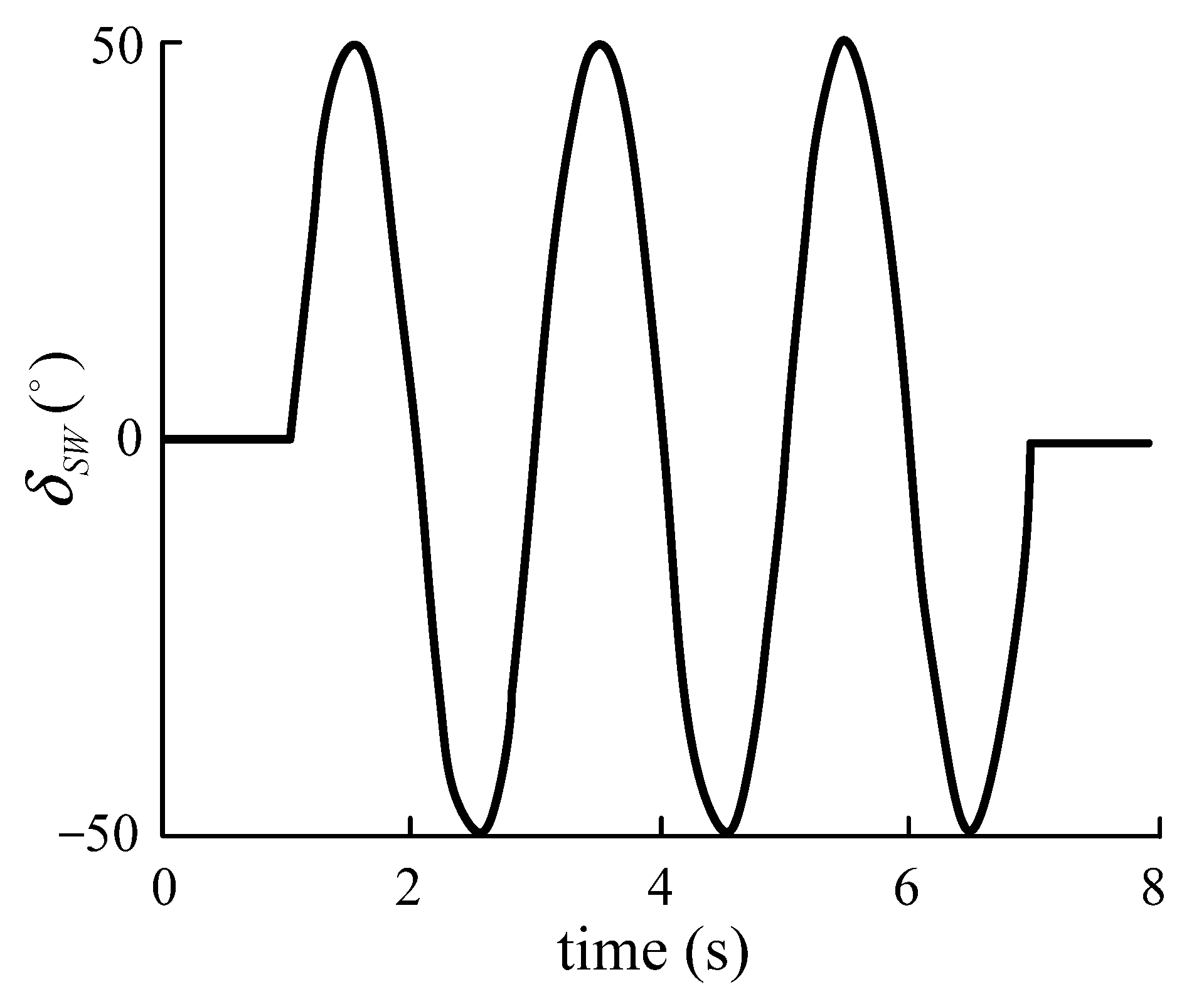
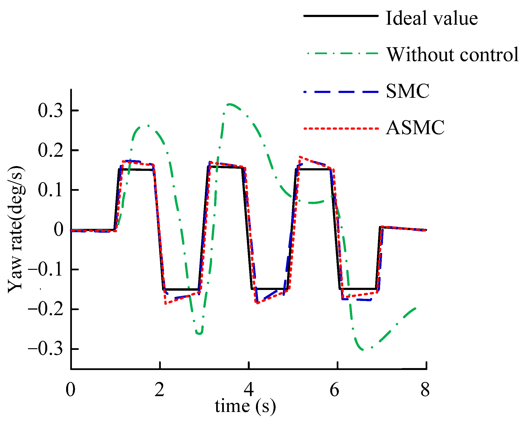
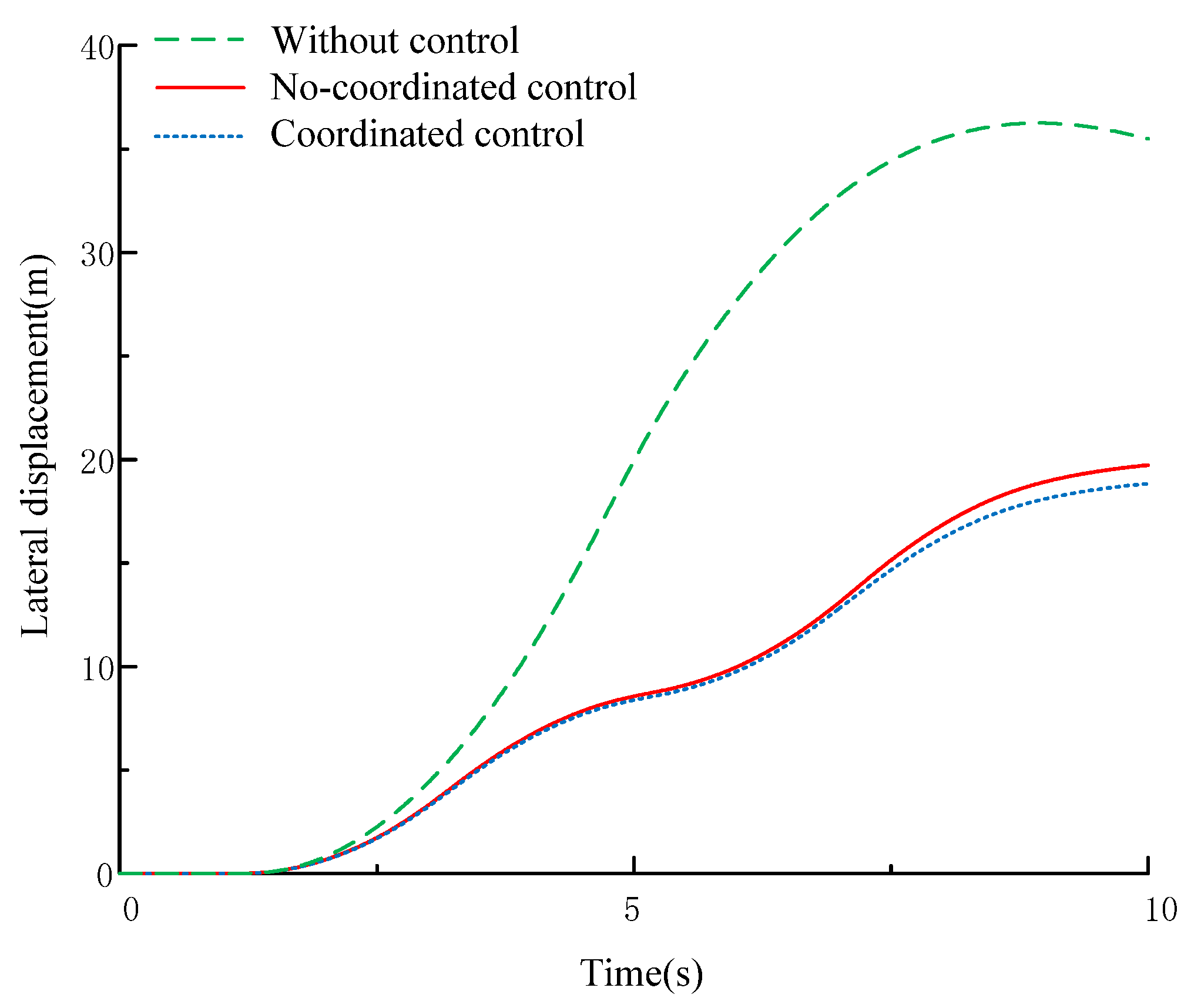
5.2. Lane Change Simulation

After verifying the effectiveness of the ASMC controller, we conducted a simulation verification of the controller effect after applying joint control. Under the condition that the value of μ is 0.85 and the value of v x is 60 km/h, the sine angle signal is input to the vehicle’s front wheel.
The steering wheel angle input is given a sine wave at (1–9), and the input of the steering wheel angle is 0 at (0–1) and (9–10), as shown in Figure 20. Judging from Figure 21, after control is applied, the lateral displacement of the vehicle decreases compared with and without the control, and the driving is more stable during steering. Judging from Figure 22 and Figure 23, the ideal value of control parameters can be followed once the control is applied compared with the vehicle without control. Compared with the non-coordinated control, the above error can be greatly reduced after the coordinated control is applied; the maximum yaw rate error is reduced from 0.046 rad/s to 0.012 rad/s, and the maximum sideslip angle error is reduced from 0.05 rad to 0.02 rad, to better follow the ideal value. Judging from Figure 24, when the vehicle is not controlled, the phase trajectory is in the unstable region and the vehicle is unstable; when the non-coordinated control is applied to the vehicle, the phase trajectory is close to the stable boundary, and the vehicle has the risk of becoming unstable; when the coordinated control is applied to the vehicle, the phase trajectory is in the stable region, and the vehicle is not unstable. Therefore, the controller designed in this paper is very effective for improving the vehicle’s stability during steering. The black solid lines and black dashed lines in Figure 24 are the boundary lines of the stability region and the boundary lines of the joint control region respectively. Figure 25 displays the optimized torque distribution of the four wheels.

5.3. Serpentine Test

In order to further verify the controller established above, a virtual test site for snake-shaped piles is established in this paper, as shown in Figure 26, and the simulated vehicle speed remains unchanged. The specific simulation comparison results are shown in Figure 27, Figure 28, Figure 29 and Figure 30.
It can be seen from Figure 27 that the vehicle has an ideal yaw response capability after applying control, and its angle input is much smaller than that without control. In addition, the yaw response of the vehicle after coordinated control is better. Figure 28 and Figure 29 can show that compared with the vehicle without control, the vehicle can effectively control its yaw rate and sideslip angle through the steering wheel angle under the control of applying yaw moment, and after coordinated control, the value of yaw rate and sideslip angle can be kept in a small range and the change trend is more stable, which can also intuitively explain that the vehicle is more stable when changing lanes continuously at high speed. It can be seen from Figure 30 that the vehicle can run well along the desired test road. At the moment, after the coordinated control of the controller, the effect of the vehicle is better than that of the vehicle without coordinated control.

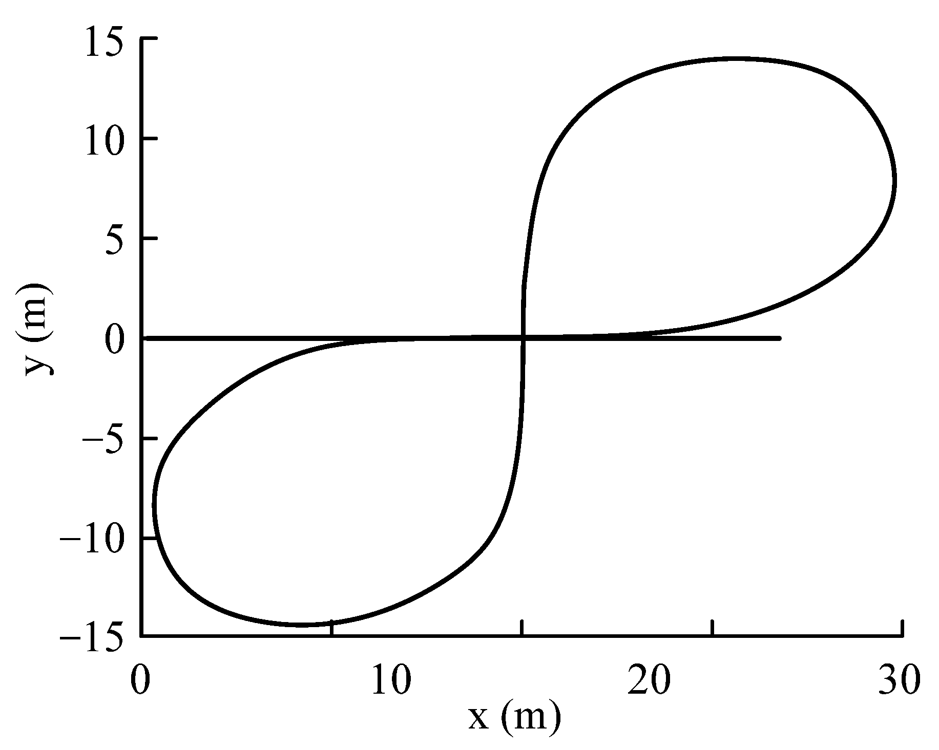
5.4. Lemniscate Test

The driving condition of the lemniscate is often used to test the steering portability of vehicles. The polar coordinate equation ( ρ , θ ) of the standard lemniscate line track path is:
ρ = 3 R 0 cos 2 θ
According to the test requirements, the simulated vehicle speed is selected as 10.8 km/h, and the corresponding minimum curvature radius R 0 of the double button line is 6 m. In order to combine the track data of the lemniscate with the driver model, it is necessary to convert its polar coordinate equation into a rectangular coordinate equation. In addition, in order to facilitate the vehicle to enter the simulation lane smoothly during the simulation, the standard lemniscate is rotated by 45° and shifted to the right for 15 m. The adjusted rectangular coordinate system parameter equation is:
{ ρ = 3 R 0 cos ( 2 ( θ + p i / 4 ) p i / 2 ) x = ρ cos ( θ + p i / 4 ) + 15 y = ρ sin ( θ + p i / 4 ) θ ( p i / 4 , p i / 4 ) ( 3 p i / 4 , 5 p i / 4 )
The comparison results of simulation tests are shown in Figure 31, Figure 32, Figure 33 and Figure 34.
As shown in Figure 32, after the vehicle is controlled, its steering wheel angle input amplitude decreases somewhat. Because the simulated vehicle speed is relatively low, the decrease in the angle input amplitude is not as large as in the serpentine condition.
Figure 33 and Figure 34 shows that although the yaw rate of vehicle does not differ significantly when the simulated vehicle speed is low, the sideslip angle is too large when no control is applied, resulting in a poor ability of the vehicle to track the desired path, which can also be reflected in Figure 35.

6. Conclusions

This paper proposes an ASMC control strategy for yaw stability based on the phase plane. Based on the ASMC theory, a yaw stability controller is designed, which can output the yaw moment required to maintain vehicle stability. The β β ˙ phase plane is used to judge the vehicle state, and different control methods are used to control the vehicle in stable and unstable states. When the vehicle is in the stable region, the yaw rate is controlled separately; when the vehicle is in the critical unstable region, the yaw rate and the sideslip angle are jointly controlled; when the vehicle is in the unstable region, the sideslip angle is controlled separately, so that the vehicle can quickly recover to a stable state. In addition, the torque optimization distribution strategy adopted by the lower controller can further reduce the error of control parameters and improve the vehicle’s lateral stability.
However, for the four-wheel independent-drive EV using differential power steering, the controller as designed and the differential power steering controller will interact with each other when working. In future scientific research, the coordination between them should be solved to improve vehicle stability further. Furthermore, torque overshoot occurs in the process of vehicle torque distribution. Therefore, a new control strategy of torque distribution can be proposed using a multi-objective optimization algorithm to control or reduce the sudden overshoot in torque in the future.

Author Contributions

Conceptualization, Z.Z.; manuscript writing, J.Z.; image description, X.Y. All authors have read and agreed to the published version of the manuscript.

Funding

This work is supported by the National Natural Science Foundation of China (51805149), the Major Project of Henan Province in 2022 (221100240400), and the major project of Ningbo Science and Technology Innovation 2025 “Development of Light Electric Vehicle Hub Motor and Control System” (2019B10073).

Data Availability Statement

Not applicable.

Conflicts of Interest

The authors declare no conflict of interest.

References

  1. Yu, Z.P.; Leng, B.; Xiong, L.; Feng, Y.; Shi, F.M. Direct Yaw Moment Control for Distributed Drive Electric Vehicle Handling Performance Improvement. Chin. J. Mech. Eng. 2016, 29, 486–497. [Google Scholar] [CrossRef]
  2. Tian, J.; Tong, J.; Luo, S. Differential Steering Control of Four-Wheel Independent-Drive Electric Vehicles. Energies 2018, 11, 2892. [Google Scholar] [CrossRef]
  3. Zhang, H.; Xiao, Q.; Wang, C.G.; Zhou, X.J. The Impact of the Lateral Non-Linear Stability of the High-Speed Railway Vehicle Caused by the Yaw Damper. In Proceedings of the 3rd International Symposium on Innovation and Sustainability of Modern Railway (ISMR 2012), E China Jiaotong Univ, Nanchang, China, 20–21 September 2012; p. 563. [Google Scholar]
  4. Aoki, A.; Marumo, Y.; Kageyama, I. Effects of multiple axles on the lateral dynamics of multi-articulated vehicles. Veh. Syst. Dyn. 2013, 51, 338–359. [Google Scholar] [CrossRef]
  5. Feng, Y.; Yu, X.H.; Han, F.L. On nonsingular terminal sliding-mode control of nonlinear systems. Automatica 2013, 49, 1715–1722. [Google Scholar] [CrossRef]
  6. Wu, B.L.; Wang, D.W.; Poh, E.K. Decentralized sliding-mode control for attitude synchronization in spacecraft formation. Int. J. Robust Nonlinear Control 2013, 23, 1183–1197. [Google Scholar] [CrossRef]
  7. Chen, M.; Mei, R.; Jiang, B. Sliding Mode Control for a Class of Uncertain MIMO Nonlinear Systems with Application to Near-Space Vehicles. Math. Probl. Eng. 2013, 2013, 9. [Google Scholar] [CrossRef]
  8. Sun, H.B.; Li, S.H.; Sun, C.Y. Finite time integral sliding mode control of hypersonic vehicles. Nonlinear Dyn. 2013, 73, 229–244. [Google Scholar] [CrossRef]
  9. Qian, M.S.; Jiang, B.; Xu, D.Z. Fault tolerant control scheme design for the formation control system of unmanned aerial vehicles. Proc. Inst. Mech. Eng. Part I-J. Syst. Control Eng. 2013, 227, 626–634. [Google Scholar] [CrossRef]
  10. Wang, Y.C.; Wang, Z.P.; Zhang, L.; Liu, M.C.; Zhu, J.N. Lateral stability enhancement based on a novel sliding mode prediction control for a four-wheel-independently actuated electric vehicle. Iet. Intell. Transp. Syst. 2019, 13, 124–133. [Google Scholar] [CrossRef]
  11. Zhang, H.Z.; Liang, J.S.; Jiang, H.B.; Cai, Y.F.; Xu, X. Stability Research of Distributed Drive Electric Vehicle by Adaptive Direct Yaw Moment Control. IEEE Access 2019, 7, 106225–106237. [Google Scholar] [CrossRef]
  12. Mousavinejad, E.; Han, Q.L.; Yang, F.W.; Zhu, Y.; Vlacic, L. Integrated control of ground vehicles dynamics via advanced terminal sliding mode control. Veh. Syst. Dyn. 2017, 55, 268–294. [Google Scholar] [CrossRef]
  13. Bagheri, A.; Azadi, S.; Soltani, A. A combined use of adaptive sliding mode control and unscented Kalman filter estimator to improve vehicle yaw stability. Proc. Inst. Mech. Eng. Part K-J. Multi-Body Dyn. 2017, 231, 388–401. [Google Scholar] [CrossRef]
  14. Zhou, H.; Liu, Z. Vehicle Yaw Stability-Control System Design Based on Sliding Mode and Backstepping Control Approach. IEEE Trans. Veh. Technol. 2010, 59, 3674–3678. [Google Scholar] [CrossRef]
  15. Zhifu, W.; Yang, Z.H.; Chaopeng, L.I.; Jun, F. Research on Straight Line Stability Control Strategy of Four Wheel Drive Vehicle Based on the Sliding Mode Variable Structure Control and Optimization Algorithm. In Proceedings of the Applied Energy Symposium and Summit-Low-Carbon Cities and Urban Energy Systems (CUE), Jinan Assoc Sci & Technol, Jinan, China, 13–15 June 2016; pp. 342–347. [Google Scholar]
  16. Le, A.T.; Chen, C.K. Vehicle stability control by using an adaptive sliding-mode algorithm. Int. J. Veh. Des. 2016, 72, 107–131. [Google Scholar] [CrossRef]
  17. Wang, H.; Han, J.; Zhang, H. Lateral Stability Analysis of 4WID Electric Vehicle Based on Sliding Mode Control and Optimal Distribution Torque Strategy. Actuators 2022, 11, 244. [Google Scholar] [CrossRef]
  18. Zhang, F.; Xiao, H.; Zhang, Y.; Gong, G. Distributed Drive Electric Bus Handling Stability Control Based on Lyapunov Theory and Sliding Mode Control. Actuators 2022, 11, 85. [Google Scholar] [CrossRef]
  19. Zhu, H.; Zhang, F.; Zhang, Y.; Su, L.; Gong, G. Yaw Stability Research of the Distributed Drive Electric Bus by Adaptive Nonsingular Fast Terminal Sliding Mode Control. Machines 2022, 10, 969. [Google Scholar] [CrossRef]
  20. Farroni, F.; Russo, M.; Russo, R. A combined use of phase plane and handing diagram method to study the influence of tyre and vehicle characteristics on stability. Veh. Syst. Dyn. 2013, 51, 1265–1285. [Google Scholar] [CrossRef]
  21. Vignati, M.; Sabbioni, E.; Cheli, F. A torque vectorring control for enhancing vehicle performance in drifting. Electronics 2018, 7, 394. [Google Scholar] [CrossRef]
  22. Cui, Y.Y.; Wang, Y. Overview vehicle pedestrian protection technology. Sci. Technol. Inf. 2017, 15, 214–215. [Google Scholar]
  23. Zhu, S.; Wei, B.; Liu, D.; Chen, H.; Huang, X.; Zheng, Y.; Wei, W.A. Dynamics Coordinated Control System for 4WD-4WS Electric Vehicles. Electronics 2022, 11, 3731. [Google Scholar] [CrossRef]
  24. Zhong, L.F.; Peng, Y.H.; Jiang, M. Stability control of distributed driven electric vehicle based on phase plane. Automot. Eng. 2021, 43, 721–729. [Google Scholar]
  25. Zhou, B.; Liu, Y.Y.; Wu, X.J. Integrated control of active front steering and direct yaw moment. J. Zhejiang Univ. (Eng. Sci.) 2022, 56, 2330–2339. [Google Scholar]
  26. Liu, X.C.; Liu, J.; Li, H.J. Research on direct yaw moment control of vehicle based on phase plane method. J. Hefei Univ. Technol. (Nat. Sci.) 2019, 42, 1455–1461. [Google Scholar]
  27. Rajamani, R.; Piyabongkarn, D. New paradigms for the integration of yaw stability and rollover prevention functions in vehicle stability control. IEEE Trans. Intell. Transp. Syst. 2013, 14, 249–261. [Google Scholar] [CrossRef]
  28. Lu, C.; Yuan, J.; Zha, G.L. Sliding Mode Integrated Control for Vehicle Systems Based on AFS and DYC. Math. Probl. Eng. 2020, 2020, 8. [Google Scholar] [CrossRef]
  29. Latin American and Caribbean New Car Assessment Programme (Latin NCAP) Testing Protocols, Version 1.0.0. [S/OL]; Latin NCAP: Leuven, Belgium, 2020.
  30. Gong, T.X.; Xie, X.Y. A control strategy of vehicle electronic stability based on phase plane method. J. Transp. Inf. Saf. 2019, 37, 83–90. [Google Scholar]
  31. Xiong, L.; Qu, T.; Feng, Y.; Deng, L.H. Stability Criterion for the Vehicle under Critical Driving Situation. J. Mech. Eng. 2015, 51, 103–111. [Google Scholar] [CrossRef]
  32. Unger, N.J.; Ombuki-Berman, B.M.; Engelbrecht, A.P. Cooperative Particle Swarm Optimization in Dynamic Environments. In Proceedings of the IEEE Symposium on Swarm Intelligence (SIS), Singapore, 16–19 April 2013; IEEE: Piscataway, NJ, USA, 2013; pp. 172–179. [Google Scholar]
  33. Xu, X.Y.; Li, G.Y.; Tao, S.Y.; Zhang, H. Simulation and Analysis on Longitudinal and Lateral Slipping Energy Consumption of Four-wheel Independently Driven Electric Vehicle Tires. J. Mech. Eng. 2021, 57, 92–102. [Google Scholar]
Figure 1. Reference model of 2-DOF vehicle.
Wevj 14 00116 g001
Figure 2. Phase plane.
Wevj 14 00116 g002
Figure 3. The structure of yaw stability controller.
Wevj 14 00116 g003
Figure 4. The block diagram of PSO.
Wevj 14 00116 g004
Figure 5. Evolution process curve.
Wevj 14 00116 g005
Figure 6. Division of β β ˙ phase plane control region.
Wevj 14 00116 g006
Figure 7. Relationship between G and β β ˙ phase plane control domain.
Wevj 14 00116 g007
Figure 8. Carsim vehicle model.
Wevj 14 00116 g008
Figure 9. Carsim vehicle body parameter setting.
Wevj 14 00116 g009
Figure 10. External input power mode diagram.
Wevj 14 00116 g010
Figure 11. Carsim/Simulink joint simulation input and output interfaces.
Wevj 14 00116 g011
Figure 12. Steering wheel angle input.
Wevj 14 00116 g012
Figure 13. Yaw rate.
Wevj 14 00116 g013
Figure 14. Sideslip angle.
Wevj 14 00116 g014
Figure 15. Lateral displacement.
Wevj 14 00116 g015
Figure 16. Steering wheel angle.
Wevj 14 00116 g016
Figure 17. The trajectory of vehicle.
Wevj 14 00116 g017
Figure 18. Control law output.
Wevj 14 00116 g018
Figure 19. The torque of FL with SMC and ASMC.
Wevj 14 00116 g019
Figure 20. Steering wheel angle input.
Wevj 14 00116 g020
Figure 21. Lateral displacement.
Wevj 14 00116 g021
Figure 22. Yaw rate.
Wevj 14 00116 g022
Figure 23. Sideslip angle.
Wevj 14 00116 g023
Figure 24. β β ˙ phase plane.
Wevj 14 00116 g024
Figure 25. The optimized torque of wheels.
Wevj 14 00116 g025
Figure 26. Front wheel angle.
Wevj 14 00116 g026
Figure 27. Steering wheel angle.
Wevj 14 00116 g027
Figure 28. Yaw rate.
Wevj 14 00116 g028
Figure 29. Sideslip angle.
Wevj 14 00116 g029
Figure 30. Vehicle running track.
Wevj 14 00116 g030
Figure 31. Simulation lemniscate path.
Wevj 14 00116 g031
Figure 32. Steering wheel angle.
Wevj 14 00116 g032
Figure 33. Yaw rate.
Wevj 14 00116 g033
Figure 34. Sideslip angle.
Wevj 14 00116 g034
Figure 35. The trajectory of vehicle.
Wevj 14 00116 g035
Table 1. The β β ˙ phase plane stability boundary parameters of different values of μ .
µck
0.30.08−1.68
0.40.10−2.02
0.50.13−2.39
0.60.15−2.83
0.70.18−2.86
0.80.20−3.03
0.90.23−3.36
1.00.27−3.79
Table 2. Optimization results of yaw rate controller parameters.
Controller Parameterscωεω
Optimization results93.20079.9821
Table 3. Optimization results of sideslip angle controller parameters.
Controller Parameterscβεβ
Optimization results46.13083.0325
Table 4. The vehicle simulation parameters.
ParameterUnitValue
Vehicle weightkg1530
Distance between the front axle and the center of massm1.2
Distance between the front axle and the center of massm1.4
Inertia of vehicle around z-axiskg m22500.6
Front and rear axle wheel trackm1.65
Height of vehicle center of massm0.6
Effective radius of wheelm0.33
Longitudinal cornering stiffnessN/rad40,000
Lateral cornering stiffnessN/rad50,000
Table 5. The main parameters of controllers.
ParameterValue
c ω 93.2007
c β 46.1308
ε ω 9.9821
ε β 3.0325
γ 0.43
τ 12
Disclaimer/Publisher’s Note: The statements, opinions and data contained in all publications are solely those of the individual author(s) and contributor(s) and not of MDPI and/or the editor(s). MDPI and/or the editor(s) disclaim responsibility for any injury to people or property resulting from any ideas, methods, instructions or products referred to in the content.

