Optimal Planning of Electric Vehicle Charging Stations Considering Traffic Load for Smart Cities

Abstract

The massive introduction of electric vehicles as a mobility alternative requires deploying an infrastructure of charging stations for electric cars (ICSEC). This new mobility concept will mitigate the environmental harm caused by the emission of CO2 generated by conventional internal combustion mobility methods. The sustainability of the ICSEC depends not only on the capacity to meet the demand for charging batteries for electric vehicles (EV) but also on an adequate number of public/private charging stations (CS) distributed in a geolocalized area. It is noted that the distribution of CS must respond to a set of real mobility constraints, such as vehicular flow capacity, road capacity, and trajectories. The planning, intelligent location of public charging stations (PCS), and contingency analysis will enable us to study the increase in demand for electrical distribution substations (EDS). Therefore, the present model explains the need to plan the massive introduction of EVs by observing the user’s conditions at the trajectory level through finite resource allocation processes, segmentation, and minimum spanning trees, by observing heterogeneous vehicular flow criteria through microscopic analysis, to understand the space–time relationship of vehicular flow in georeferenced scenarios. Consequently, the computational complexity of the model is of the combinatorial type, and it is defined as NP-Hard given the multiple variables and constraints within the transportation problem.

1. Introduction

The energy supply for charging EVs plays an essential role in the sustainability of the mass introduction of EVs. This new mobility concept contributes directly to reducing greenhouse gases and decreasing noise and visual pollution compared to conventional mobility. In Europe, it is estimated that approximately 80% of noise pollution caused on the streets is generated by vehicles that use fossil fuels as an energy source. Furthermore, it is kept in mind that human mobility has a fundamental role in the development and economic growth of towns; however, with conventional mobility, the environmental cost becomes critical and necessary for future generations due to the current radical climate change.

The most challenging problem is managing the supply chain for EV recharging; therefore, it is essential to plan the deployment of CS to EVs [1]. Consequently, two optimizing variables are identified, (i) operating costs and (ii) heterogeneous charge balance [2]. Therefore, studying and simulating the EV flow that should serve each CS in different zones within a geolocalized area is essential to plan, predict demand, and guarantee electric service continuity. Forecasting the peak demand in the CS is necessary because it would help us decide whether an electricity grid can take on new charges. If not, creating new supply circuits for each electric mobility CS is necessary. It would significantly contribute to maintaining the voltage stability in EDS and guaranteeing service continuity. Therefore, the planning can be divided into three stages: (i) planning to satisfy demand, (ii) allocation and location of CS, and (iii) EV routing to an energy source to recharge the vehicle’s battery.

The article considers features in the model that bring the transport problem closer to different real-world scenarios. Microscopic examination in traffic models considers fundamental aspects such as speed and spacing between vehicles; it lets us know vehicle flow or density in geolocated scenarios. In addition, consider microscopic analysis to understand the space–time relationship in vehicular networks [3].

Therefore, a multi-objective approach to address the problems of routing, siting, and sizing of CS that are required for electric mobility charging infrastructures (CI) is noticed in this article. Capacities are allocated to each deployed CS to satisfy the demand, and the sum of the needed parts must equal the resource allocated in the planning problem. Candidate sites for siting CS could be parks, shopping malls, green spaces, and car parks.

Finally, the best topology for EV routing decisions is achieved by looking at road capacity, vehicle flow, and spacing variables. Hence, the aim is to solve multiple resource allocation problems in a georeferenced area of NP-hard computational complexity, which is supported by optimization tools, graph theory, and routing algorithms; it has been possible to reduce the computational complexity to a problem of NP-type [4].

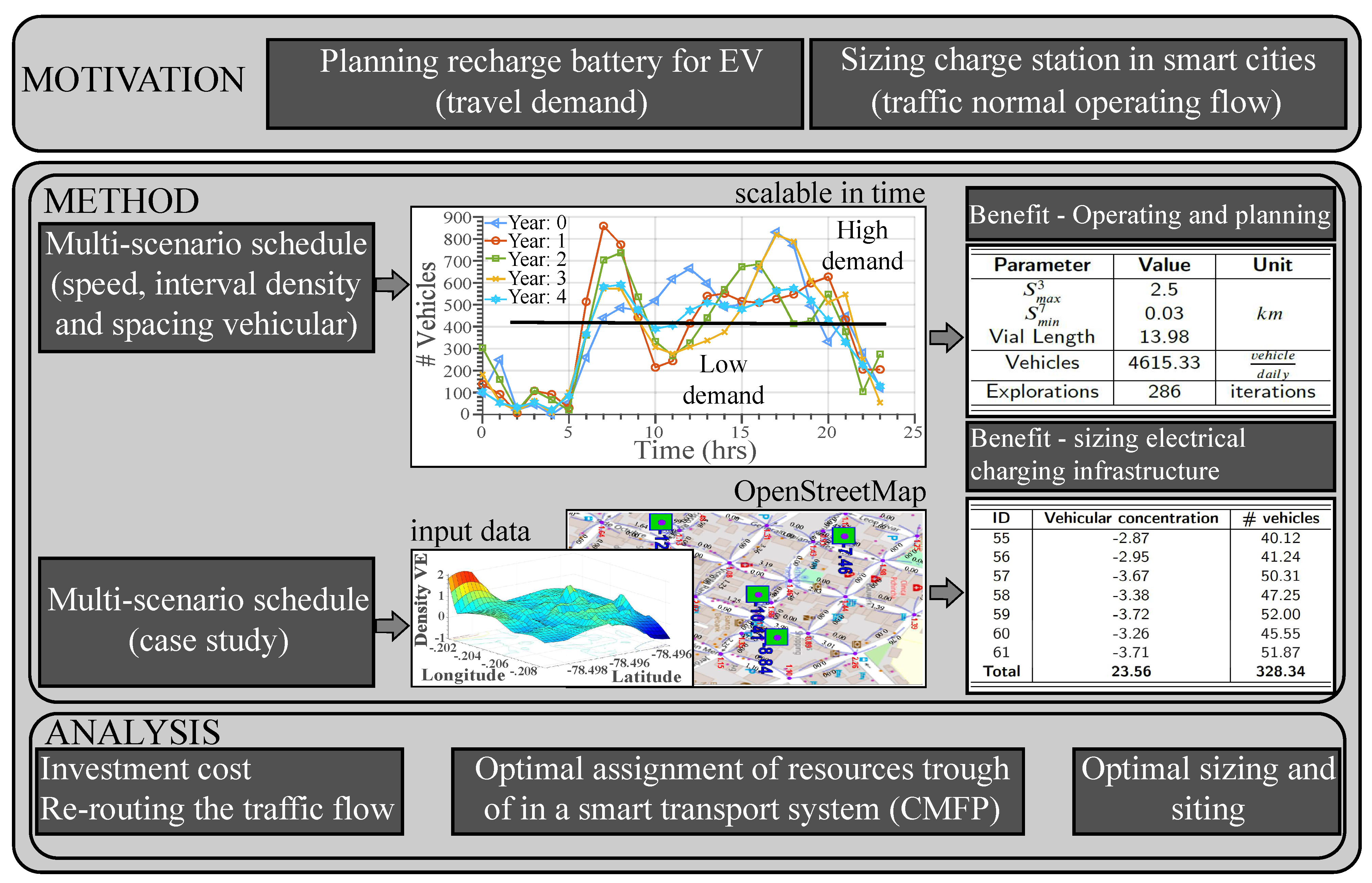
Figure 1 presents the architecture proposed in this article. It shows a spatial approach on two levels: (I) route-based demands and (II) equipment for charging infrastructure. These demands must be covered by spreading a set of CS in permitted areas. Moreover, the equipment for a charging infrastructure should consider the forecast of vehicle demand as a function of the traffic density generated in georeferenced scenarios. Consequently, the heuristic proposed in this paper will solve the resource allocation by considering the required charging infrastructure equipment for EVs using real transport constraints at the level of trajectories under a spatial approach.

Level I analyzes the flow generated on each road section as a function of vehicular density. Vehicular flow helps to understand traffic characteristics and behavior, which are essential requirements for planning, road and street design, and operation within the land transport system. There are microscopic and macroscopic models that relate different variables such as volume, speed, density, interval, and spacing [5] for understanding traffic density in geolocated scenarios.

Capacity and levels of service concepts applied to different road elements can be understood using the above models. However, it is not a trivial problem because these transport evaluation strategies are a great challenge to solve as they involve geographical elements (roads, orography, flyovers), vehicle arrangements are unknown, and due to their high traffic variability, it is not possible to predict with certainty trajectory patterns [6]. Then, to develop optimal routes at the level of trajectories, it is essential to pay special attention to the aspects related to the variables of vehicular flow, the probabilistic description of vehicular traffic, the distribution of vehicles in viability, and the statistical distribution of vehicular density.

Consequently, level I studies and assigns a weight to each road section by observing actual mobility criteria for vehicle flow analysis with microscopic analysis. Level II examines the different topologies generated to achieve connectivity or supply of the multiple resources developed in the other CS to satisfy the EV demand in vehicle flow management processes [7,8,9,10]. Vertices are defined as each track section’s CS, EV, and intersections. Edges constitute the geolocated topology [11,12] of connection and the connectivity relationship between the multiple vertices that are part of a directed graph.

Henceforth, the present article is organized as follows: Section 2 briefly reviews related work. Section 3 presents the traditional problem formulation and the methodology to solve it. Section 4 contains the results analysis and the proposed model’s validation. Finally, in Section 5, conclusions are presented.

2. Related Works

The work proposed in this article represents a significant advance in electro-mobility infrastructure planning. By considering actual transport variables at the trajectory level, the current job has developed a heuristic model that can plan and allocate resources to deploy electric vehicle charging stations. The model considers the complex interplay between vehicular flow, road capacity, and trajectories and uses advanced optimization algorithms such as multi-commodity flow problems and graph theory to provide finite and scalable solutions over time.

One of the key contributions of this work is its potential to become a computational model and infrastructure manager for planning and resource allocation in electro-mobility. The scalable model has been validated through iterative processes that deal with contingency concepts to predict the maximum density of vehicular traffic in road networks. Moreover, the model provides hourly analysis of vehicle flow and allows for the identification of maximum and minimum demands experienced for each charging station, which contributes to coordinating and managing battery-charging processes in electric vehicles. Overall, this work represents a significant step forward in developing sustainable transportation systems and has important implications for the future of electro-mobility.

This paper studies the optimal deployment and allocation of CS resources to satisfy demand at the trajectory level by considering vehicular flow characteristics with heterogeneous users. This paper is closely related to three lines of research: optimal CS location, Resource allocation for EV charging at the trajectory level, and ICSEC planning. This section summarizes the most current and relevant work on the proposed study.

2.1. Assignment and Location Problem

The location of energy supply centers for EVs was developed in [13,14] by considering the routing problem and EV autonomy as the decision variables.

Table 1. Category L7e-C EV Characteristics.

Vehicle Electric	Autonomy (km)	Voltage Terminal (V)	Engine (kW)	Maximum Speed (km/h)	System Regenerative	Vehicle Category Dimensions (m)
Tazzari Zero	200	230	15–25	90	✓
Renault Twizy	100	230	17	80	✓	height < 2.5
Audi Urban	73	230–400	15	100	-	width < 1.5
Peugeot BB1	120	230	15	60	-	length < 3.7

sets out brief characteristics of designed vehicles for urban usage of the L7e-C category, in which the average range is observed to be 123 km. The decision problem is determining the optimal supply for charging infrastructures, the locations and users’ allocation to each CS, and the optimal dispatch policy. In one paper [15], the problem is expanded to a dynamic planning model by considering itineraries by EV usage.

Recently, in [16], the location problem was studied by analyzing supply and demand, including the driver’s psychological component, and in [17], in addition to deploying CS, it is suggested to involve the integration of distributed generation sources.

The authors showed that integrating distributed generation helps relieve unexpected charges on existing distribution electrical grids, which have generally been operated in cities for several years. However, it has not been possible to demonstrate a rigorous analysis considering the road capacity in each section and vehicle flow analysis that defines city traffic in decision variables to allocate and locate CS in electric mobility infrastructures.

2.2. Resource Allocation under Optimal Criteria

Both exact and approximate solutions have been applied to solve the resource allocation problem. Accurate solutions involve integer linear programming problems, while approximate solutions involve heuristics and metaheuristics development.

Table 2. Taxonomy of related studies.

Author, Year	Model		Problem		Obj. Function	Constraints	Solution		Trajectories		Other
	Theoretical	Experimental	Location Allocation	Route			Exact	Heuristic/Meta	Density Traffic	Urban Study
Gan, 2020 [18]	✓	-	✓	✓	Maximize Profit Service	Distance Standy time Power grid capacity	-	✓	-	-	Elastic demand Stochastic Newton-Raphson NILP
Inga, 2019 [19]	✓	-	✓	✓	Minimize Costs Flows	Capacity Distance	-	✓	-	✓	Scalable multi-commodity capacities network
Demir, 2019 [20]	-	✓	-	✓	Minimize Travel distance Costs	Flows # Vehicles	-	✓	-	-	Deterministic ILP Demand fluctuation NP-hard
Azadi, 2019 [21]	✓	-	-	✓	Maximize User Routes Service	Capacity Operation Schedule	✓	-	✓	-	Multiple commodity flows network Heterogenous traffic MILP Branch and Bound Algorithm
Bevrani, 2019 [22]	✓	-	-	✓	Minimize Flow Routs	Congestion Expanstion tree Conservation flow	✓	-	-	✓	Multi-commodity network flow Flow reduction functions NLP Multiple nodes
Campaña, 2019 [23]	✓	-	✓	✓	Minimize # Charging stations Trajectory Costs	Distance Minimal tree Coverage	-	✓	✓	✓	ILP Graph theory Homogenous nodes
Liu, 2019 [24]	✓	-	-	✓	Minimize Power losses in distribution Maximize Flow	Capacity Congestion	✓	-	✓	-	Heterogeneous nodes Optimal Solution Charging congestion during fuzzy multi-objective model
Ghasemi, 2019 [25]	✓	-	✓	✓	Min. Transportation cost Minimize shortages Max. humanitarian	Demand Heterogenous flow Capacity Distance	✓	✓	✓	-	Probability approach Planning periods Multiple-objective PSO Stochastic demand
Campaña, 2019 [26]	✓	-	✓	✓	Min. Trajectories Min. Charging Station Min. Congestion road	Coverage Distance Capacity	-	✓	✓	✓	Segmentation ILP Need for Users Neighborhood analysis
Current study	✓	-	✓	✓	Min. Trajectories Min. flow Min. Charging stations Max. Humanitarian	Capacity Distance Coverage Demand	✓	✓	✓	✓	Revised-Simplex MILP Multi-commodity network flow Heterogeneous nodes Scalable Multi-objective NP-Hard Non convex

provides a taxonomy of related studies with a summary of the problem statement, objective function, main constraints, solution methods, and other fundamental characteristics to address the problem of allocation and CS display.

Recent developments focused on solving planning problems based on a convex multi-objective model, which will depend on the number of variables and constraints considered. Among the issues that need to be adequately considered are those features that bring the problem closer to real-world situations, such as the heterogeneous vehicular fleet and the multiple CS options, which are used to route the vehicular flow to ensure continuity of coverage for EV battery recharging.

2.3. Planning of Charging Infrastructure for Batteries in Electric Mobility

The technological advancement and the constant effort to introduce new concepts of electric mobility on a large scale have encouraged the scientific community to develop products that enable the reduction of CO₂ emissions by conventional private and public transport. Today there are multiple electric mobility alternatives, such as bicycles, cars, and public transport buses. However, it has not been possible to introduce EVs massively into the land transport system because of variables that do not make large-scale purchases attractive to potential users in urban and rural areas. These unattractive variables to consumers could be limited autonomy, long charging times, battery life, high costs, and lack of charging infrastructure for EVs.

This article focuses on the problem of planning and deployment of CS to support the mass introduction of electric vehicles into the vehicle fleet. The spatial-temporal collaboration between CS, allocation, and optimal routing based on bidirectional flows, undoubtedly, gives place to ICSEC. In one paper [27], the authors proposed tackling the problem by modeling the hybrid vehicle traffic with different charge terminals and observing EV driving range constraints. Furthermore, the mathematical formulation and solution are addressed by linear programming.

In another paper [28,29,30,31,32], the problem of allocation and deployment of CS is addressed by partially considering several aspects which guide the achievement of robust results; these aspects are limited capacity, probability of trajectories, travel time, flow conservation, charge time, spatial, temporal collaboration, terminal type, and traffic events.

Planning, CS deployment, and selecting the charging terminal are important because EVs present technical constraints such as maximum driving ranges and limited payload. Airports have been classified into three types, depending on the charge current which EVs can withstand.

Table 3. Types of charging terminals for ICSEC [23].

Type	Current (Amp) Type	Time (h)	Recharge (%)	Power kW	Owner	INEC Standard
Slow	16 AC	8	100	4–8	Public-Private
Semi-fast	32 AC	1.150	50–80	22	Public
Fast	63 AC	0.500	50–80	50	Public	61,851
Ultra-fast	250–400 DC	0.170	50–80	350	Public
Change-Battery	AC-DC	0.033	100	-	Public

briefly overviews the different types of existing terminals and their various applications. It is well-known that as the charging current increases, the charging time decreases, and the types of terminals differ. Type I and II application are in residential areas, and type III is exclusively a public/private service.

Consequently, this article is essential because it covers the planning problem in its integral form at both levels, as explained in the previous paragraphs. Remember that to dimension CS, it is necessary to model the vehicular traffic at the trajectory level and the user’s need for battery recharging. Therefore, it has to consider ICSEC an essential actor during the planning process.

To look for integrated solutions that safeguard the operability of existing electricity grids, according to their lifetime and the fact that many of them have reached their nominal capacities, they could be affected by the massive introduction of EVs in the traditional electricity distribution system.

It will allow us to decide whether or not the existing networks can support new charges, thus making it possible to choose to use the existing equipment or whether it is necessary to install new distribution circuits to satisfy the demand for battery recharging in electric mobility, to guarantee the quality, continuity, and safety of the electricity service. In [33,34], a method of clustering and constructing minimum spanning trees is proposed as an indispensable tool in electrical equipment’s optimization and planning processes.

3. Problem Description

This section describes the problem through the stochastic analysis of vehicular traffic at the trajectory level and allocating resources for ICSEC. Furthermore, the strategy and methodology proposed are presented in this paper, followed by the formal problem statement.

3.1. Stochastic Analysis of Vehicular Traffic and Resource Allocation at ICSEC

Service stations in the field of public-private transport have an important role because they supply primary energy to provide autonomy to the electric mobility vehicle fleet. The massive introduction of EVs in daily traffic has to be planned, which implies having heterogeneous vehicle networks where the main actors are conventional vehicles and EVs from the public and private sectors.

Most research focuses on users and reducing travel times by reorganizing vehicle traffic according to road capacity and considering heterogeneous traffic networks to allocate resources. A fundamental detail is that the demand for vehicle charge is not focused on the nodes (electric or conventional vehicles) but on the flow of the vehicular traffic network. Consequently, the research objective is to solve the problem of location and allocation of resources to CS by considering heterogeneous vehicle density.

Therefore, the vehicular traffic flow can simulate the demand generated by EVs displayed on a heterogeneous road network. It is assumed that installing a service center for EV battery charging cannot satisfy the induced demand due to the limited capacity of the CS on a road section.

This limitation will cause critical traffic flow because of high coincidence factors due to battery recharging requirements. Consequently, battery capacity is fundamental to CS deployment and resource allocation. Therefore, it will obtain the following considerations: (i) if there is a CS between a start and end point of a trajectory, the EV’s autonomy must be greater than the length of the route, and (ii) if there is only one CS in the route, the EV’s autonomy must be more than double the route length.

An important detail already exposed is that the algorithm must obtain knowledge of the multiple options at the trajectory level that an EV can take in terms of spatial and temporal constraints (distance, trajectory, and flow variability). In addition, it considers that the maximum demand for battery recharging in a given area will be provided by the maximum vehicle density traveling in a given time interval. This maximum demand or traffic density occurs when the vehicle spacing and the speed with which the vehicle is traveling are the minimum.

Based on microscopic models for vehicle density analysis, it studied the maximum allowable density in a georeferenced area by considering vehicle spacing and speed variables. Using a random vector under Poisson distribution, it simulates the vehicular traffic density within a time interval considering maximum traffic density at minimum speeds and spacing. The objective is to select and allocate resources to CS to maximize traffic flow and provide users with coverage in a given area.

The deployment planning of CS can consider the location of the different charging infrastructures and their influence on the power quality, security, and economics of the system’s operation. Consequently, it is defined as a typical multi-objective optimization problem. This article will solve the planning problem by considering a multigraph in levels: (i) traffic and (ii) distribution networks. These categories can overlap, meaning two nodes of each type can be located in the same area. In level 1 of the traffic network, the vehicle flow is characterized. Therefore, in level 2, the capacity of the charging station is studied according to the number of EVs that can be supported.

3.2. Proposed Strategy and Methodology

This paper proposes a theoretical model of location and assignment of CS with traffic flow restrictions in heterogeneous scenarios. The main objective is to optimize resources using the maximum vehicle flow capacity on each road section in georeferenced areas. A non-convex combinatorial problem is proposed under a mixed integer linear programming structure. Consequently, it will use the column generation algorithm to solve the multi-product flow problem frequently used in MILP.

The column generation algorithm divides the problem into two stages (i) restricted master problem (RMP) and (ii) sub-problem. Solving RMP with the minimum number of variables obtains dual costs for each restriction master problem; this solution is used in the objective function of the sub-problem and solved. If the accurate value of the sub-problem is a negative reduced cost variable, this is added to RMP and is again solved. This process is iterative, and the stopping criterion happens when the objective value of the sub-problem is greater than or equal to zero. When this happens, the restricted master problem can be considered optimal.

At the first level, CS display and location are performed by assuming that a driver will choose the shortest path from the starting point to the destination by observing distance and traffic flow constraints. These restrictions will reduce to an optimal number the vector length of candidate CS sites located at strategic locations, such as shopping centers, parks, car parks, customer service centers, and conventional charging stations.

At the second level, the capacity of the CS must satisfy the daily EV charging demand, which is determined by the charging time of the simulated vehicles and the number of EVs that it may be able to handle in a specific time interval. Different locations and capacities of the CS will cause other impacts on the distribution grid. An additional detail is that the Dijkstra algorithm is used to find the shortest path between the multiple ways generated in the function of the vehicle density.

Four main groups are proposed to guide the methodological development of this article: (i) scenario analysis, (ii) process, (iii) simulation, and (iv) solution. Figure 2 shows a solution to the transport and resource allocation problem flowchart. In scenario analysis, the model suggests having full knowledge of the case study, which means that the model knows the coordinates of the electrical equipment (charging stations) and, based on the positions of each vehicle, the maximum vehicle density at the trajectory level is known. Figure 2 reveals that the georeferenced data are extracted from a free database published in OpenStreetMap.

Once the scenario has been characterized, the experimental procedure defined by the process and simulation detailed in Figure 2 is carried out. This process explains the actions, considerations, and variables that enter the simulation. After the iterative process, the proposed heuristic returns the hourly local optimum in the function of the incoming vehicular traffic density variables. It used Matlab software for the simulation.

Finally, this article considers basic research because of its experimental nature by implementing simulation processes. It has a quantitative approach to determining the allocation of resources and minimization of economic and social impacts. This model is exploratory; therefore, it is essential to analyze different study cases.

3.3. Problem Formulation

The product flow problem considers two necessary restrictions: (i) travel demand, which means that all products or EVs must be transported to their destinations or CS, and (ii) the capacity of each intersection of each road section; this means that the traffic flow at each intersection does not have to exceed its capacity. Therefore, the multi-product problem would appear to be a combination of several single-product problems, given both the limited roadway capacity and the diversification of vehicle density. Some considerations and the formal description of the problem statement are presented in this section.

Furthermore, the interaction between EVs denotes multiple complexities to solve the single-product flow problem independently. Consequently, the demand generated by each EV is related to various supply options for this demand, and its origin-destination node pair, which refers to the position of the EV and the CS, respectively, can identify it. The located CSS provides the battery recharging supply.

The optimal collection of CS is selected based on spatial-temporal collaboration, which involves minimum displacements by observing traffic flow constraints. Moreover, it assumes that the shortest or available route depending on the nodal traffic flow and capacity at the trajectory level can acquire the essential product supply. The variables are detailed below in

Table 4. Notation used in this article.

Nomenclature	Description
m	Number of nodes $\{\nu \cup \epsilon \cup \zeta \cup \beta \}$
$G_{m\times m}$	Directed graph matrix
${\phi }_{1,2,\cdots ,m}$, $\phi$	EV autonomy vector
$\mathcal{V}$	Nodes vector
$\mathcal{A}$	Edges Vector
$\nu$	EV nodes
$\epsilon$	CS nodes
$u,v$	Origin and destination edges, respectively
$i,j$	Origin and destination transversal intersection edges
$\iota$	Road cross length
$\alpha$	Number of heterogeneous vehicles in $\iota$
$\varpi$	Discrete probability of the number of vehicles
$\beta$	Intersections vector
$W_{\beta }$	Total vehicle concentration
${\mathcal{S}}_{1,2,3\cdots }$	Set of paths $u,v$
$f_{\beta }$	Flow rate
$\kappa$	CS candidate sites vector
${\delta }_{\kappa }$	Fixed cost to install EDS
$n_j$	Number of vehicles to cover capacity $\psi$
$\psi$	CS capacity
$\mathcal{M}$	Set of enabled paths edges
$\mathcal{L}$	Set of edges of a path $u,v$
${\varphi }_j$	Location variable
${\theta }_k$	Subset of assigned arcs
${\tau }_e^j$	Route enabled
$q,Q$	Partial and total vehicular flow rate
$V_e$	Constant travel speed
$t_s$	Time in hours
t	Number of commodities
$\Theta$	Incremental annual rate given as a percentage
s	Average spacing between vehicles
k	Index vector
${\chi }_{\ast }^k$	Revised simplex reduced negative value
${\mathsf{\Psi }}_p$	Partial solution to the primary problem
P	Identification for each iteration
${\pi }_{1,2,\cdots }$	Dual variables
$np$	Number of periods in years

.

Consider $G(\phi ,\mathcal{V},\mathcal{A})$ a directed graph where $\phi$ corresponds to the autonomy constraint of an EV towards a CS; the distance computation is performed with the haversine equation and it is given in km. The vertices set $\mathcal{V}$ represent the multiple nodes located in the study area, such as electric vehicles ($\nu$), charging stations ($\epsilon$), the intersections ($\zeta$); therefore, $\nu ,\epsilon ,\zeta \in \mathcal{V}$ and the displacement is between two nodes origin-destination ${\nu }_{u,v},{\epsilon }_{u,v},{\zeta }_{u,v}\in \mathcal{V}$ and the set of edges $u,v\in \mathcal{A}$ represent the origin and destination, respectively. $\mathcal{A}$ allows the construction of a specific topology; that is, it relates the multiple nodes existing in G leading to the creation of spanning trees at each level. On each track section ($\iota$), there is a certain number of vehicles ($\alpha$). Each track section is limited in capacity ($\varpi$), and it is formed between two vertices in a set of corners ($\beta$). At each $\beta$, it reflects a demand or cumulative cost ($W_{\beta }$). Consequently, the multiple paths (${\mathcal{S}}_{1,2,3\cdots }$), where $\mathcal{S}\in \mathcal{V}$, is formed from a set of intermediate nodes $\beta$, which, dimension the total flow $f_{\beta }$ by assigning a weight $W_{\beta }$ on each path. A track section can be either unidirectional or bidirectional ${\beta }_{i,j}\ne {\beta }_{j,i}$. In other words, $\{\beta \cup \mathcal{S}\}\in \mathcal{V}$. Consider $\kappa \subseteq \mathcal{V}$ a subset of candidate sites where $\kappa \notin \beta ,\nu$ because the selected positions to locate CS are parks, shopping centers, public car park. Moreover, $u=\{i\in \mathcal{V}:\exists \beta \in \mathcal{S}|i=1,2,3\cdots \}$ denotes the subset of source nodes in a trajectory and $v=\{j\in \mathcal{V}:\exists \beta \in \mathcal{S}|j=1,2,3\cdots \}$ it denotes the subset of destination nodes, where m is the length of the vector $\{\nu \cup \epsilon \cup \zeta \cup \beta \}$. In other words, the different trajectories (products) are constructed only from the charge nodes $\beta$ to $\zeta$. This is possible, since ${\sum }_{i=1}^m{\sum }_{j=1}^m{\beta }_{i,j}$, $\forall (i\ne j),\in {\mathbb{Z}}^{+}$. Finally, consider ${\delta }_{\kappa }$ the cost to install a node ${\zeta }_j$ where $j\in \kappa$ and it is $n_j$ the maximum number of vehicles to cover the capacity $\psi$ of each CS.

Consider $\mathcal{M}\subseteq \mathcal{A}$ subsets of assigned edges that define the enabled roads in the whole studied scenario. Therefore, it is $\mathcal{M}={\beta }_{i,j},{\beta }_i\in u$ y $j\in \kappa$. Consider $\mathcal{L}\subseteq \mathcal{A}$ a subset of edges of a path ${\mathcal{L}}_i,{\mathcal{L}}_j$ where $i,j\in \{\kappa \cup \beta \}$ with this it guarantees that there are no arcs from other families. Next, it defines the set of binary variables of resource selection.

• ${\varphi }_j$ location variable $\epsilon$, is 1 when it is found any node that is part of the set j, $j\in \kappa$, 0 in any other way.
• ${\theta }_k$ subset of assigned arcs, if the arc $k\in \mathcal{M}$ it is used, otherwise 0.
• ${\tau }_e^j$ path enabled, is 1 if the edge $e\in \mathcal{L}$ and $j\in \kappa$, otherwise 0.

$$\begin{array}{cc}{\displaystyle f_{\beta \left(m\right)}=\sum _{m=1}^{\mathcal{S}}{W}_{\beta \left(m\right)}}\hfill & [\frac{veh}{km}]\hfill \end{array}$$

(1)

$$\begin{array}{cc}{\displaystyle W_{\beta (m,n)}=\sum _{m=1}^{V_e}\sum _{n=1}^{np}\frac{q_{\left(n\right)}}{V_{e\left(m\right)}}}\hfill & [\frac{veh}{km}]\hfill \end{array}$$

(2)

$$\begin{array}{cc}{\displaystyle q_{\left(m\right)}=\sum _{m=1}^{np}\frac{{\alpha }_{\left(m\right)}}{t_s}}\hfill & [\frac{veh}{hra}]\hfill \end{array}$$

(3)

$$\begin{array}{cc}{\displaystyle {\alpha }_{\left(m\right)}=\sum _{m=1}^{np}{\varpi }_{(m-1)}\ast \mathsf{\Theta }}\hfill & [veh]\hfill \end{array}$$

(4)

$$\begin{array}{cc}{\displaystyle \varpi =\sum _{m=1}^{np}\frac{{\displaystyle \sum _{n=1}^{\mathcal{A}}\frac{{\iota }_{\left(n\right)}+s_{\left(n\right)}}{s_{\left(n\right)}}}}{np}}\hfill & [veh]\hfill \end{array}$$

(5)

Equations (1) and (2) are used to calculate vehicles’ total and partial concentration in a specific area. The Equation (3) expresses the current flow rate on a road section and represents the frequency at which a certain number of vehicles pass through at a given time.

Equation (4) calculates the average number of vehicles that may be on a lane in the function of the cross-sectional length of the road and the spacing s between cars and $\Theta$ it is an annual rate of increase under a discrete Poisson probability distribution.

Finally, with Equation (5), the number of vehicles as a function of cross-sectional length and spacing is calculated. It assumes that the spacing between cars is uniform and that the maximum capacity of a road-cross section occurs at the minimum distance s between vehicles and minimum speed (V). It is essential to mention that a microscopic model has been used for the traffic flow analysis, which considers the spacing s and the individual speeds ($V_e$). Therefore, the multi-product transport problem can be formulated as follows:

Objective function:

$$\begin{array}{c}{\displaystyle \mathrm{M}\mathrm{i}\mathrm{n}:Z_{\left(Q\right)}=\sum _{k=1}^t{Q}_k{\theta }_k}\hfill \end{array}$$

(6)

Subject to:

$$\begin{array}{cc}{\displaystyle \sum _{k=1}^t{\theta }_k^i=1,}\hfill & i=1,2,\cdots ,u\left(k\right)\hfill \end{array}$$

(7)

$$\begin{array}{cc}{\displaystyle \sum _{k=1}^t{\theta }_k^j=1,}\hfill & j=1,2,\cdots ,v\left(k\right)\hfill \end{array}$$

(8)

$$\begin{array}{cc}{\displaystyle \sum _{k=1}^t{\theta }_k^i=f_{\beta }{|}_k^i,}\hfill & i=1,2,\cdots ,u\left(k\right)\hfill \end{array}$$

(9)

$$\begin{array}{cc}{\displaystyle \sum _{k=1}^t{\theta }_k^j=f_{\beta }{|}_k^j,}\hfill & j=1,2,\cdots ,v\left(k\right)\hfill \end{array}$$

(10)

$$\begin{array}{c}{\displaystyle \sum _{k=1}^t{\theta }_k=\phi }\hfill \end{array}$$

(11)

$$\begin{array}{cc}{\displaystyle \sum _{k\in \mathcal{S}}{\theta }_k\le \left|\mathcal{S}\right|-r\left(\mathcal{S}\right),}\hfill & \forall \mathcal{S}\subseteq \mathcal{V},\mathcal{S}\ne 0\hfill \end{array}$$

(12)

$$\begin{array}{cc}{\theta }_k,\hfill & \in \{0,1\}\hfill \end{array}$$

(13)

where Equation (6) corresponds to the objective function; consequently, Equations (7) and (8) guarantee that the origin and destination of the route are from service nodes to demand response. Equations (9)–(11) correspond to the corresponding routing’s vehicle concentration and electric vehicle autonomy restrictions.

Equation (12) ensures that dual variables are searched and aggregated. Finally, the binary variable is declared with Equation (13). Furthermore, $Q_k={[q_1,q_2,\dots ,q_m]}^T$ where $k=1,2,\dots ,t$ and represents the flow rate of each basic product.

The accumulated capacity and autonomy vector of the EV is represented by $f_{\beta }={[W_{\beta 1},W_{\beta 2},\dots ,W_{\beta m}]}^T$ and $\phi ={[{\phi }_1,{\phi }_2,\dots ,{\phi }_m]}^T$, respectively.

The adjacency matrix between vertices and edges is represented by $G={\left[G_{ij}\right]}_{m\times m}$. The length of $m\times m$ is a function of the total number of vertices in the scenario. Finally, $f_{\beta }{|}_k^i=[f_{\beta }{|}_k^1,f_{\beta }{|}_k^2,\dots ,f_{\beta }{|}_k^m]$ and $f_{\beta }{|}_k^j=[f_{\beta }{|}_k^1,f_{\beta }{|}_k^2,\dots ,f_{\beta }{|}_k^m]$ with $k=1,2,\dots ,t$ is defined as follows.

$$\begin{array}{c}\hfill f_{\beta }{|}_k^i=\left\{\begin{array}{ccc}-W_{\beta }{|}_k^i\hfill & si\hfill & i=u\left(k\right)\hfill \\ W_{\beta }{|}_k^i\hfill & si\hfill & i=v\left(k\right)\hfill \\ 0\hfill & \hfill & \mathrm{a}\mathrm{n}\mathrm{y}\mathrm{o}\mathrm{t}\mathrm{h}\mathrm{e}\mathrm{r}\mathrm{c}\mathrm{a}\mathrm{s}\mathrm{e}\hfill \end{array}\right.\end{array}$$

(14)

$$\begin{array}{c}\hfill f_{\beta }{|}_k^j=\left\{\begin{array}{ccc}-W_{\beta }{|}_k^j\hfill & si\hfill & j=u\left(k\right)\hfill \\ W_{\beta }{|}_k^j\hfill & si\hfill & j=v\left(k\right)\hfill \\ 0\hfill & \hfill & \mathrm{a}\mathrm{n}\mathrm{y}\mathrm{o}\mathrm{t}\mathrm{h}\mathrm{e}\mathrm{r}\mathrm{c}\mathrm{a}\mathrm{s}\mathrm{e}\hfill \end{array}\right.\end{array}$$

(15)

Column Generator

This article used the column generation method. This method allows us to solve extensive linear programs. The idea is to take advantage by generating variables that have the potential to improve the objective function. The algorithm process is as follows. We first consider the following assumptions: (i) the variables are non-basic, (ii) The variables will assume a value higher or equal to zero in the optimal solution, (iii) an initial subset of variables must be considered to solve an initial problem, and (iv) the problem can be divided into the primal and dual problem.

The primal problem is solved with a subset of variables considered; with this solution, it obtains dual costs for each restriction of the primal problem. It assumes that ${\chi }_{\ast }^k$ is the optimal value of the dual objective function, which was solved by the revised simplex method; if the real double deal is a negative reduced cost such that ${\chi }_{\ast }^k<0,\forall k=1,2,\dots ,t$ this variable is added as a column to the primal problem, and it is again solved iteratively.

When ${\chi }_{\ast }^k\ge 0,\forall k=k_1,k_2,\dots ,k_p$, the algorithm stops, and it can conclude that the primal problem is optimal.

For each linear problem, there is a problem that is solved in parallel; the last one is known as a dual problem. We consider the following issue to solve the primal and dual problems.

$$\begin{array}{c}z=cx,\hfill \end{array}$$

(16)

Subject to:

$$\begin{array}{c}Ax\le b\hfill \end{array}$$

(17)

$$\begin{array}{c}x\ge 0\hfill \end{array}$$

(18)

The linear problem is defined according to Equations (16) and (17) with a dual counterpart.

$$\begin{array}{c}z=wb,\hfill \end{array}$$

(19)

$$\begin{array}{c}wA\le c\hfill \end{array}$$

(20)

$$\begin{array}{c}w\ge 0\hfill \end{array}$$

(21)

Equations (19)–(21) have the same terms, except for the term w, which is a variable that is assigned to Equation (17) of the first formulation, where $w=C_{BV}{B}^{-}1$, which corresponds to an iteration of a revised simplex. It is known as a dual variable arrangement. The variables $C_{BV}$ y $B^{-}1$ correspond to primary variable coefficients and connectivity matrix that relates vertices and edges, respectively. Consequently, the problem illustrated in Equations (6)–(12) can be separated into two primal and dual issues, respectively. The equations defining each primal and dual problem are presented as follows.

Primal—Primary Problem

Objective function:

$$\begin{array}{c}{\displaystyle \mathrm{M}\mathrm{i}\mathrm{n}:z_{\left(Q\right)}=\sum _{p\in P}\sum _{k=1}^t{Q}_k{\mathsf{\Psi }}_p{\theta }_{pk}}\hfill \end{array}$$

(22)

Subject to:

$$\begin{array}{cc}{\displaystyle \sum _{p\in P}{\mathsf{\Psi }}_p\sum _{k=1}^t{\theta }_{pk}=f_{\beta }{|}_k^i,}\hfill & i=1,2,\cdots ,u\left(k\right)\hfill \end{array}$$

(23)

$$\begin{array}{cc}{\displaystyle \sum _{p\in P}{\mathsf{\Psi }}_p\sum _{k=1}^t{\theta }_{pk}=f_{\beta }{|}_k^j,}\hfill & j=1,2,\cdots ,v\left(k\right)\hfill \end{array}$$

(24)

$$\begin{array}{c}{\displaystyle \sum _{p\in P}{\mathsf{\Psi }}_p\sum _{k=1}^t{\theta }_{pk}=\phi }\hfill \end{array}$$

(25)

$$\begin{array}{c}{\displaystyle \sum _{p\in P}{\mathsf{\Psi }}_p=1}\hfill \end{array}$$

(26)

The new set P is used in each iteration to identify the generated routes, and ${\mathsf{\Psi }}_p$ is a partial solution to the primal problem. Equation (22) is the objective function of the main problem, and Equations (23)–(25) are vehicular concentration and autonomy restrictions, respectively, that permit restricting the solution space to routes that only fulfill a little value. With Equation (26), a non-zero solution to the second problem is guaranteed.

Dual-secondary problem

Objective function:

$${\displaystyle \begin{array}{c}\mathrm{M}\mathrm{i}\mathrm{n}:\hfill \\ {\displaystyle {\chi }_{\ast }^k=\sum _{k=1}^t{Q}_k{\theta }_k-{\pi }_3\sum _{k=1}^t{\theta }_k^i-{\pi }_2\sum _{k=1}^t}\hfill \end{array}{\theta }_k^j-{\pi }_1\sum _{k=1}^t{\theta }_k-{\pi }_0}$$

(27)

Subject to:

$$\begin{array}{c}{\displaystyle \sum _{k=1}^t{\theta }_k^i=1}\hfill \end{array}$$

(28)

$$\begin{array}{c}{\displaystyle \sum _{k=1}^t{\theta }_k^j=1}\hfill \end{array}$$

(29)

$$\begin{array}{cc}{\displaystyle \sum _{k\in \mathcal{S}}{\theta }_k\le \left|\mathcal{S}\right|-r\left(\mathcal{S}\right),}\hfill & \forall \mathcal{S}\subseteq \mathcal{V},\mathcal{S}\ne 0\hfill \end{array}$$

(30)

$$\begin{array}{c}{\theta }_k\in \{0,1\}\hfill \end{array}$$

(31)

Equation (27) is the objective function of the secondary problem, so ${\chi }_{\ast }^k$ is the reduced cost variable, which, as long as ${\chi }_{\ast }^k\ne 0$ could find dual variables which are inserted into the main problem. Equations (28) and (29) are restrictions that enable source and demand nodes so the model can search for the best route. In Equation (30), the coefficient r is selected from the set $\mathcal{S}$ that will allow verifying the cost of the negative reduced variable. Finally, the binary selection variable is declared with Equation (31). Figure 3 presents the flowchart for resource location and allocation required to ICSEC.

4. Analysis of Results

This section presents the results obtained by the heuristic model MP-LRAC for creating ICSEC.

Table 5. Simulation Parameters.

Approach	Description	Consideration
Deployment	Density EV	Variable
	Study cases	A–B
	Study areas	0.99 y 2.13 km2
	Geographical area	Urban
	Geographic reference	Latitude–Longitude
Allocation	Annual rate	Variable
	Scalability	4 years
	Spacing	Variable
Application	Charging terminal	AC–DC
	Safety distance	3–6 m
	Vehicular flow	Variable
	Vehicular concentration	Variable
	Traffic speed	[20 40 60] km/h
Traffic	Light	4.3 (m) ≤
	Buses	15 (m)
	Trucks	12 (m)

shows the simulation parameters, where the need to consider input variables through heterogeneous and scalable vehicular traffic analysis in georeferenced areas is noted.

The microscopic model was used to simulate the input variables, which allows us to study the relationship between speed, length, and spacing. It has tried to recreate scenarios close to reality to determine the average number of vehicles circulating in a given area. Therefore, it will be possible to deploy charging stations for electric cars and allocate resources for the energy supply by recharging batteries in electric mobility.

Information, such as connectivity matrix, track direction, and weights assigned for each section in the optimization model, are essential. Consequently, the model’s longitudinal relationships are well-known from an intersection i to a meeting j. Case study A is illustrated in Figure 4, and here it can find the topology analyzed in this article.

Considering the actual data of case A will allow us to approach reliable solutions. Moreover, it will permit an understanding of the maximum load capacity admitted in a given time interval in this study case. It means the maximum traffic capacity on each road section is determined according to the topology (longitudinal characteristics of each road section, road direction, spacing, and vehicular speed).

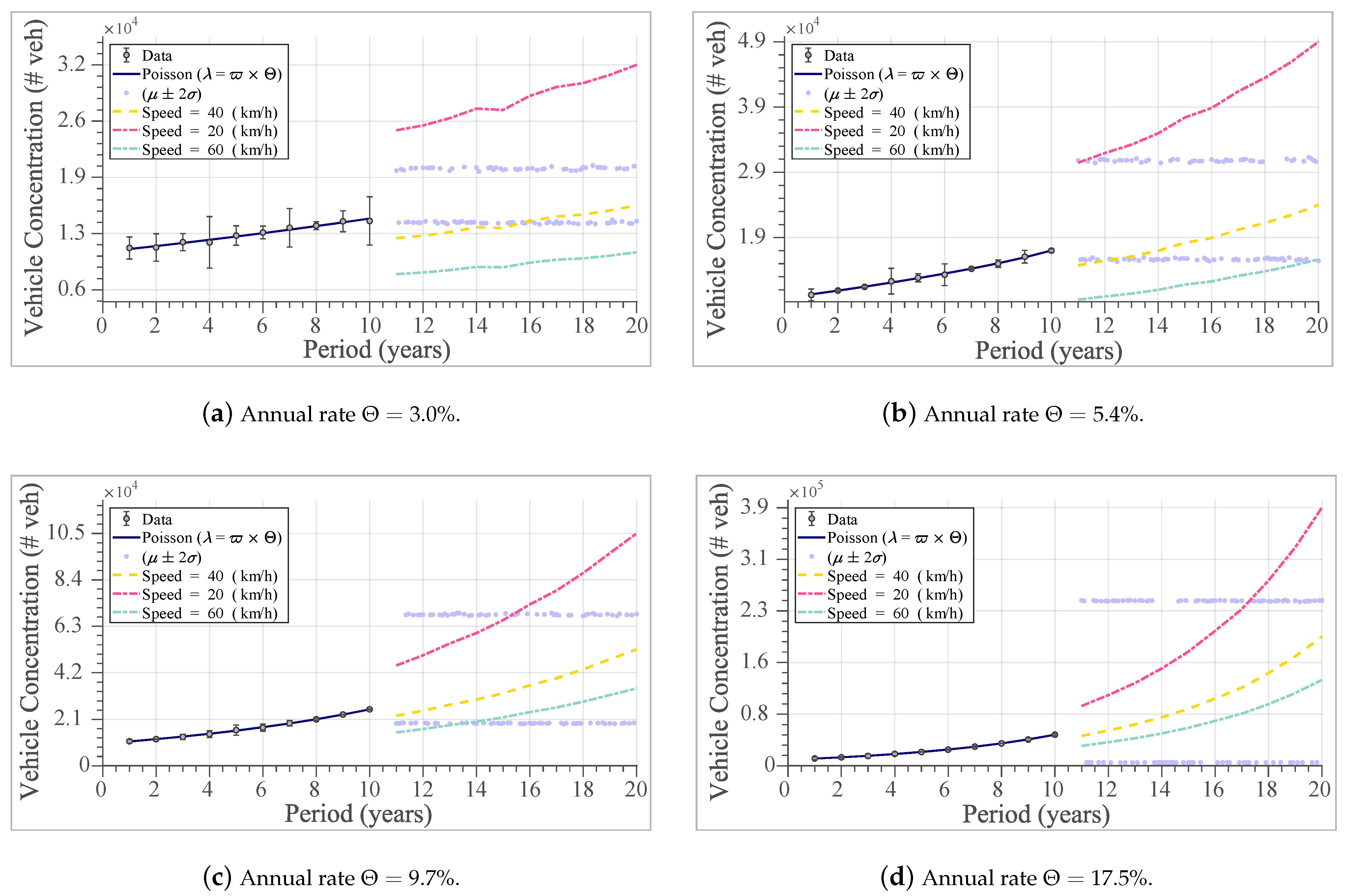
The maximum number of vehicles circulating in study case A is determined according to the complete vehicle density. Figure 5 presents the variation in vehicular concentration in the function of different incremental rates during a 20-year analysis period. The total rate corresponds to a theoretical value, which the vehicular network designer can adjust. Its value will depend on studies and estimated projections in each area of its different central governments.

This analysis of the increase in the vehicle fleet was performed over 20 years with four annual rates $\Theta$ as shown in Figure 5. There is a technically linear trend in the first ten years of analysis, which does not occur from the 11th year onwards. The literature suggests that discrete Poisson probability has recreated the scenario’s randomness.

The slopes cease to be continuous as the annual rate of the vehicle fleet increases, and they adopt exponential trends in their addiction. Therefore, a first reflection is that it is necessary to generate control policies that mitigate for this unfavorable impact by not obtaining control over the increased vehicle fleet.

The number of heterogeneous vehicles deployed in each case in Figure 5 responds to the maximum capacity at the trajectory level that involves variables explained in previous paragraphs, such as cross-section, spacing, and speed. Consequently, it can be inferred from Figure 5 that as the average speed with which vehicles circulate on each section of the road increases, the inverse happens with the vehicle concentration. It means that as the speed increases, the vehicle density decreases.

This phenomenon is because the flow rate is inversely proportional to the speed. The purple color represents the empirical values that indicate the number of values above and below the average value of the three speeds analyzed from 11 to 20 years. It means that approximately 95% of data are above and below average, and their values are visualized in Figure 5. Therefore, speed, geometric road layout, spacing, and annual growth rates of the vehicle fleet are considered in this article as fundamental variables to achieve results that satisfy near-optimal solutions in real scenarios.

Figure 6 illustrates the number of vehicles distributed over 24 h for case study A. The trend in Figure 6 corresponds to the weekly average vehicle traffic behavior under standard working day conditions. The proposed model in this article is evaluated over four years from year zero, and an incremental rate of 3% will be considered. The total rate is taken as a reference from the literature to adapt this variable to any required reality or case study.

The hourly variability of the number of vehicles that circulate in a given area responds to a normalized random vector by considering the original trend (year zero) and the annual rate of increase. Moreover, Figure 6 shows that the highest vehicle density is distributed from 07:00 to 20:00 h. Consequently, the charging stations should be designed to meet the demand during peak traffic hours in a given area.

Consequently, in Figure 7, we illustrate the estimated number of vehicles counted in a specific hour from 0:00 to 24:00 h through the frequency graph. It is correct to think that the number of cars that circulate in a particular time will follow the base mobility pattern curve, Year: 0. Finally, Figure 7 presents the zones of highest vehicle concentration illustrated by the edges, which in turn are randomly distributed in case study A.

The adjacency matrix allows us to understand the data distribution within the case study. Figure 8 presents two techniques for reordering the sparse adjacency matrix: (i) Cuthill-McKee inverse algorithm and (ii) Column Permutations. In the solid blue color in Figure 8, the inverse Cuthill-McKee algorithm is illustrated, which has a clear tendency to group its non-zero elements closer to the diagonal while preserving the special relationship from each edge ($i,j$) to its nodes $i=j$ and $j=i$.

The column permutation algorithm illustrated in Figure 8 using a heat graph permits reordering columns of the sparse-type matrix A in non-decreasing order of non-zero count. This metric allows us to visualize the different magnitudes of vehicle density that will be considered to evaluate the model and the relationship between each node in the scenario.

Therefore, Figure 8 shows that the input data are stochastic and that their origin is the result of a microscopic analysis that allows us to understand the interaction of the different variables involved in vehicular mobility, such as spacing, speed, the topology of the study area, and lengths of the vehicles. It has enabled us to bring the problem closer to the stochastic reality of land transport mobility by considering its possible trajectories within a geolocated area. Hence, it uses the microscopic model to solve PM-UARC as a directed graph to model the traffic rate and the maximum vehicle concentration at the trajectory level.

The discrete Poisson distribution generates different case studies based on a typical curve of vehicle traffic operation during working hours from Monday to Friday. This base curve is considered to be year 0. The scalability analysis of the vehicle traffic evaluated in the proposed model’s performance is based on it, and its results are shown in Figure 9.

Figure 9 illustrates the algorithm performance evaluated in a scalable scenario from year 0 to year 4. Figure 9a shows the machine time to solve the primary problem. It is easily observed that it depends on the time of day; the machine time spent to solve the primal problem is variant; this response to the stochasticity of the vehicular flow in each time interval.

The linear problem is constructed as the primary concern. In Figure 9a, the time trend of the machine is a function of the annual growth rate of the vehicle fleet. It is increased with a minimum of 3 min at year 0 and a maximum of 4.7 min at year 4. In Figure 9c, the observer’s machine time is presented, which has the function of deciding the growth of the column generator; this means they are the one who verifies whether the cost in terms of objective function decreases to be able to add it as a solution. Next, if a non-zero vector exists, it is added to the solution. Once added, the algorithm repeats the iterations from the primary and secondary problems, and the observer makes decisions based on the negative variables. Therefore, the time of the machine is higher than the time spent on the secondary problem, as illustrated by comparing Figure 9a,b.

A curious thing to note in Figure 9d is that the cost of the objective function in each scenario tested maintains the same trend; this means there is no data deviation from year 0 to year 4. The movement in Figure 9d responds to the immutability of the scenario topology. Finally, Figure 9d shows that the objective function is inversely proportional to the hourly characteristic curve that defines the vehicle density.

This inverse behavior of the objective function with the hourly distribution of vehicular density is linked to the operating costs; this means that the design and sizing of charging stations for electric vehicles must be according to the maximum demand that occurs from 07:00 to 20:00 h on ordinary days from Monday to Friday. Therefore, the objective function has a minimum cost in high-demand hours because it manages to justify the charging station sizing. The accurate function cost is maximum, whereas traffic demand is minimum. It is because, in those low-demand hours, the charging infrastructure is not used, so there is an oversizing in low-demand hours.

Table 6. Case A: Maximum partial demand in each CS at hour 19:00 with 32.97 km of road network in contingency N-0 corresponding to year 0.

ID	Longitude	Latitude	Concentration Vehicular	Vehicles (#)
1	−120.625225787882	35.1271587155963	−0.77	25.41
2	−120.622727167999	35.1269678899083	−1.31	43.22
3	−120.617829873029	35.1267623853211	−0.64	21.22
4	−120.609994201077	35.1261458715596	−1.48	48.71
5	−120.615391220024	35.1256174311927	−1.29	42.44
6	−120.620588349380	35.1256467889908	−1.43	47.10
7	−120.624546163274	35.1248688073394	−1.09	36.03
8	−120.624326284724	35.1243403669725	−0.85	28.06
9	−120.619488956631	35.1240174311927	−1.43	47.11
10	−120.610473936095	35.1246045871560	−1.44	47.52
11	−120.611033626948	35.1230192660550	−0.67	22.00
12	−120.620568360421	35.1230779816514	−0.64	21.00
13	−120.622167477145	35.1233128440367	−0.85	27.90
14	−120.625865434572	35.1238266055046	−0.62	20.30
15	−120.625805467695	35.1222559633028	−0.61	20.19
16	−120.623466759484	35.1219183486239	−1.18	38.89
17	−120.620868194807	35.1221678899083	−0.92	30.32
18	−120.617310160094	35.1218889908257	−0.86	28.35
19	−120.615671065451	35.1218743119266	−0.99	32.73
20	−120.613552235790	35.1218449541284	−1.44	47.43
21	−120.610833737358	35.1199220183486	−1.21	39.74
22	−120.614731584375	35.1193642201835	−1.34	44.03
23	−120.616150800468	35.1204357798165	−0.96	31.70
24	−120.619588901427	35.1209495412844	−0.85	28.00
25	−120.625925401449	35.1213018348624	−0.97	32.00
26	−120.623666649075	35.1200247706422	−0.79	26.12
27	−120.619688846222	35.1195550458716	−0.81	26.78
28	−120.624606130151	35.1191293577982	−1.37	45.32
29	−120.617350138012	35.1186743119266	−1.19	39.35
30	−120.617250193216	35.1176027522936	−0.80	26.32
31	−120.618829320982	35.1176321100917	−1.09	36.00
32	−120.622327388818	35.1168981651376	−0.94	31.02
33	−120.613552235790	35.1176027522936	−0.61	20.19
34	−120.616050855673	35.1232541284404	−0.87	28.53
35	−120.608654940820	35.1195550458716	−0.62	20.31
Total			−34.92	1151.34

presents the resulting metric for case study A. In each column, respectively, it can be seen the ID of the charging station, the geographical coordinates in latitude-longitude, the vehicle concentration, and the number of vehicles to be served in the hour of maximum demand. The charging station has ID 4 experiments with a complete vehicle charge of 48.71 per 1 h.

According to what has been analyzed in the preceding paragraphs, the demand in year 0 occurs at 19:00 h, with 1151.34 vehicles distributed in the geographical area under study. The distribution of vehicle charges to be handled by each charging station during the hour 19:00 in year 0 is presented in Table 6. A percentage pattern allocates vehicle charges for the day’s remaining hours (see Figure 6). However, in this case, it has considered the maximum vehicle demand in a time interval to estimate the maximum power installed at the different charging stations.

The installed power of a CS should be directly proportional to the number of vehicles estimated to be met in the peak hour of vehicle charging. For example, if it considers the time 19:00 in Figure 6 and looks at Table 6, which illustrates the vehicle charge distribution, it observes that the charging station with ID 4 should serve 48.71 vehicles. If it assumes that all users want to charge their cars simultaneously and that the CS topology has ultra-fast charging terminals with 350 kW power, for each terminal, it should assign a design power for the EC with ID 4 of 17.05 MW.

However, it is essential to remember that the model performs the analysis for 1 h; it will determine where the maximum vehicle demand occurs by considering the topology of the geolocated area involved; this means that the 48.71 vehicles will be distributed over 60 min. Here, a fundamental detail must be analyzed in the design of the CS topology, which will necessarily involve the battery charger technology. It means that the charging times and terminals are studied to satisfy the 1-h high demand for charging batteries for electric vehicles.

The model’s adaptability to any scenario will be verified by analyzing case study B. This study case is in Arroyo Grande County, San Luis Obispo County, California, United States. It will simulate scenarios where the CSS goes out of operation for any condition and analyze the redistribution of the vehicle flow. Furthermore, it will explore what happens with the different vehicle flows in each hourly interval with a growth rate of 3.0%, as well as verify contingencies of up to N-2.

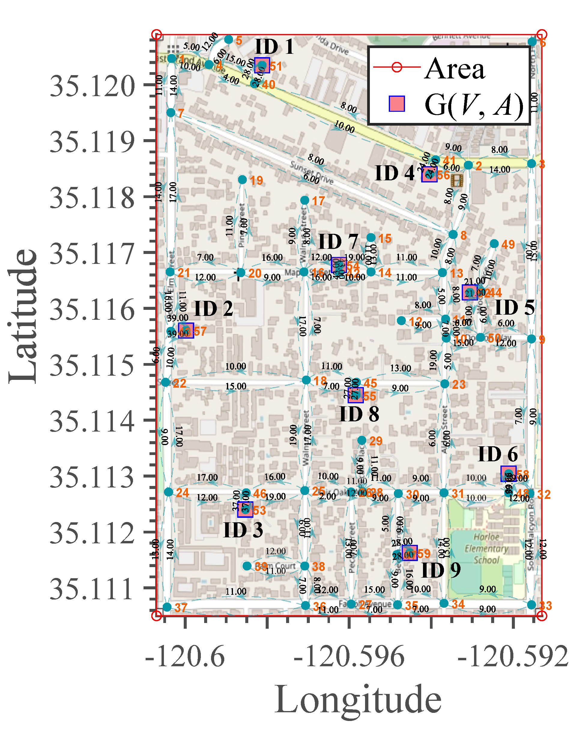
In addition, how it affects the sizing of the charging stations in EV charging infrastructures. Figure 10 presents the geographical area in which Case B will be analyzed, where nine EV charging stations are identified with ID tags.

The vehicular density analysis has been studied with microscopic examination. An additional detail visualized in dark green is the bi-directionality of each road section and how this is related to each intersection. Moreover, Figure 10 identifies the costs directly associated with the vehicle density on each path. Consequently, a case study involving traffic variables such as vehicle spacing and travel speed in vehicular networks is presented in Figure 10. These variables are entered through a random vector with the Poisson distribution.

Figure 11 presents the graphical solution to the transport problem. The magnitude of the vehicle density generated at each link is visualized in black; in red, at each intersection, the resulting vehicle density can be easily identified, which is the sum of the flows that enter each node minus the flows that leave.

A fundamental condition for the convergence of the model is that the supply centers with a negative sign cover the demand with a positive signal at each intersection. This condition is critical to maintaining the nodal equilibrium criterion, which satisfies the equations in the mathematical problem statement. The red negative sign indicates the flows that will have to be served by each charging station; let us remember that the negative sign indicates that it is a supply node (charging station).

A fundamental criterion for equipment sizing in planning algorithms is considering the worst-case scenario. This consideration will allow us to approach the optimal sizing of the resources required in the planning processes. Consequently,

Table 7. Case B: Maximum partial demand in each CS with 9984 km of road network in contingency N-0.

ID	Vehicle Concentration	# Vehicles
1	−3.00	29.95
2	−5.33	53.21
3	−4.84	48.32
4	−2.93	29.25
5	−2.18	21.77
6	−3.72	37.14
7	−3.55	35.44
8	−4.72	47.12
9	−4.62	46.12
Total	−34.89	348.34

presents the result of the analysis case in Figure 10, where the case of the highest conflict is considered.

The highest conflict occurs at maximum vehicle density moving through the geolocated area. These extreme conditions occur at minimum travel speeds with minimum vehicle spacing distances. It means that vehicle density in a geolocated area is inversely proportional to vehicle speed and spacing. Column one in Table 7 presents the charging station index; column two illustrates the resulting vehicle concentration to be served by each charging station.

The sign in column two is negative because the model considers it a node contributing to the transport system to form the balance equations. The supply nodes must cover the sum of the partial flows observed at each intersection. Consequently, with a positive sign, it denotes those consumption nodes, and with a negative character, it identifies the nodes that satisfy the equilibrium equations of the multiple-product problem.

In addition, in Table 7, the third column shows the number of vehicles each charging station will have to serve in critical conditions of high vehicle density, without considering contingencies, in a time interval where the speed and vehicle spacing variables are minimal.

Finally, the last row of Table 7 identifies the maximum number of vehicles in an instant of time according to the scenario topology, which in this case is 348.34 vehicles as the maximum admissible density in the area considered for the analysis. Consequently, with the number of cars each charging station serves and the maximum traffic density at the trajectory level, it can size and foresee the necessary resources for constructing charging infrastructure in geolocalized areas.

Moreover,

Table 8. Case B: Optimal sizing of charging stations for EVs based on multi-product flow problem.

Contingency	Deactivated	ID	ID	ID	ID	ID	ID	ID	ID	ID
	(ID)	1	2	3	4	5	6	7	8	9
N − 0	−	−3.00	−5.33	−4.84	−2.93	−2.18	−3.72	−3.55	−4.72	−4.62
N − 1	1	−	−5.60	−4.38	−4.97	−4.08	−3.90	−4.20	−4.16	−5.08
	2	−4.01	−	−5.98	−4.99	−3.65	−5.96	−4.48	−5.03	−4.93
	3	−4.27	−6.38	−	−3.62	−4.03	−4.56	−4.35	−5.11	−5.12
	4	−4.42	−4.32	−4.06	−	−3.55	−5.34	−4.72	−5.24	−5.68
	5	−4.41	−5.12	−4.81	−4.65	−	−5.24	−3.40	−5.48	−4.75
	6	−3.74	−4.37	−4.99	−6.05	−3.15	−	−4.34	−5.15	−5.79
	7	−4.25	−4.05	−5.31	−4.91	−3.53	−4.89	−	−5.53	−4.91
	8	−3.15	−4.98	−4.79	−4.73	−3.88	−5.12	−3.94	−	−4.85
	9	−4.02	−4.72	−5.41	−4.20	−3.35	−4.00	−4.86	−4.86	−
	Average ($\mathsf{\mu }$)	4.03	4,94	4.97	4.77	3.65	4.88	4.29	5.07	5.14
	Std. deviation ($\sigma$)	0.40	0.72	0.57	0.65	0.31	0.65	0.43	0.40	0.36
	$\mu +2\ast \sigma$	4.83	6.37	6.10	6.07	4.26	6.18	5.14	5.87	5.86
N − 2	1, 2	−	−	−4.67	−5.18	−4.89	−5.40	−5.54	−4.95	−5.42
	2, 3	−4.05	−	−	−4.25	−4.59	−5.42	−4.43	−6.08	−5.02
	8, 9	−4.13	−5.40	−5.49	−5.56	−5.12	−5.76	−5.46	−	−
	4, 5	−4.46	−4.89	−5.09	−	−	−6.08	−5.64	−5.71	−6.11
	7, 9	−4.83	−4.01	−7.10	−5.73	−4.31	−5.70	−	−5.93	−
	5, 7	−4.38	−4.20	−4.71	−4.25	−	−5.62	−	−6.31	−5.16
	3, 7	−5.37	−4.68	−	−5.09	−4.97	−5.13	−	−5.90	−6.14
	3, 5	−4.15	−5.03	−	−5.51	−	−4.95	−4.36	−5.80	−4.78
	2, 4	−5.20	−	−6.08	−	−5.22	−4.91	−5.06	−5.41	−6.00
	5, 6	−4.19	−4.94	−5.38	−6.36	−	−	−4.89	−6.11	−5.79
	7, 8	−4.30	−6.30	−4.50	−4.78	−5.27	−5.06	−	−	−5.46
	1, 3	−	−5.22	−	−4.25	−3.51	−5.89	−4.41	−5.69	−5.09
	3, 4	−4.77	−6.39	−	−	−3.84	−5.58	−5.07	−5.50	−6.08
	Average ($\mathsf{\mu }$)	4.53	5.11	5.38	5.10	4.64	5.46	4.98	5.76	5.55
	Std. deviation ($\sigma$)	0.43	0.74	0.81	0.68	0.59	0.36	0.47	0.36	0.47
	$\mu +2\ast \sigma$	5.39	6.58	7.00	6.46	5.82	6.19	5.93	6.48	6.50
Increment N − 1 (%)		61.0	19.5	26.0	107.2	95.4	66.1	44.8	24.4	26.8
Increment N − 2 (%)		79.7	23.5	44.6	120.5	167.0	66.4	67.0	37.3	40.7

presents the optimal sizing of charging stations by considering events or contingencies (N-1 and N-2) generated in a geolocated area from normal operation conditions (N-0). These contingencies respond to removing one or two charging stations at maximum vehicle density. The out-of-service charging stations are randomly selected. Column two in Table 8 shows the rates of charging stations that go out of service, and columns 3 to 11 present the flux density at each charging station.

Considering the contingency analysis for out-of-service charging stations, the traffic density to satisfy the battery-charging requirement must be routed or rearranged with the charging stations enabled. The experience with charging station ID 1 manifests the increased traffic density generated by operating one or two charging stations. If one looks at column three in Table 8 in normal operating conditions, the vehicle density to be served by the charging station ID 1 is $29.95\approx 30$ vehicles in a time interval when the vehicle density is maximum. When the model experiences the operation exit of the charging station with ID 4, the number of vehicles to be served given contingency N-1 is 48.22 × 48. If the charging infrastructure experiences the operation exit of two charging stations with ID 3 and 7 of contingency N-2, the traffic density to be served is 53.81 × 54 vehicles in a given time interval.

The increase represents approximately 61% and 79.7% of the different traffic densities that will have to be served when the charging infrastructure disconnects charging stations in N-1 and N-2 contingencies, respectively. Likewise, it will perform the analysis for the charging station with ID 5, which presents an increase in vehicle density of 95.4% in contingency N-1 and an increase of 167.6% in contingency N-2 that it will have to serve if one or two charging stations are taken out of operation.

If one pays attention to detail, the charging station with ID 5 in contingency N-2 experiences some increases in vehicle density that exceeds 100% in the regular operation in contingency N-0. It is understood that the algorithm reorganizes the vehicle flow in the function of a cost and capacity vector for each road section, satisfying the mathematical variables of the linear equation; however, the balance equations are fulfilled for each iteration.

The charging stations as a set will give rise to the charging station infrastructure. Therefore, if the designer of the charging infrastructure knows which percentage would increase or reduce the vehicle density to be served by each charging station, they will be able to make intelligent decisions to foresee the electrical, civil, and logistical equipment required for the location of charging infrastructures in electric mobility to guarantee coverage in the road network. To determine the sizing of the charging stations, consider the empiric rule to assess the magnitude of values within a band around the average in a normal distribution with a width of two times the standard deviation. Consequently, the green color in Table 8 indicates the optimal sizing for each charging station for electric vehicles.

By multiplying the cumulative length in kilometers of the road network times the vehicle density considering the empirical sizing criteria, one can obtain the number of vehicles each charging station will have to serve in each event studied. Furthermore,

Table 9. Maximum partial demand at each charging station with 9984 km of road network given a contingency.

Events	ID 1	ID 2	ID 3	ID 4	ID 5	ID 6	ID 7	ID 8	ID 9
N-0	29.95	53.22	48.32	29.25	21.77	37.14	35.44	47.13	46.13
N-1	48.22	63.60	60.90	60.60	42.53	61.70	51.32	58.61	58.51
N-2	53.81	65.70	69.89	64.50	58.11	61.80	59.21	64.70	64.90

allows us to verify how much the sizing of the charging station should increase given a circumstance. Consequently, the information presented makes planning the charging infrastructure for electric mobility in smart cities possible.

Once the number of electric vehicles that will circulate through each scenario studied has been identified in detail, the energy required to implement the charging infrastructure is determined. For the load forecast, it is assumed that the input power of each charger is 52.63 kVA with a power factor of 0.95, so the active power consumed by each charger is 50 kW. In addition, the charging time is assumed to be 0.5 h. 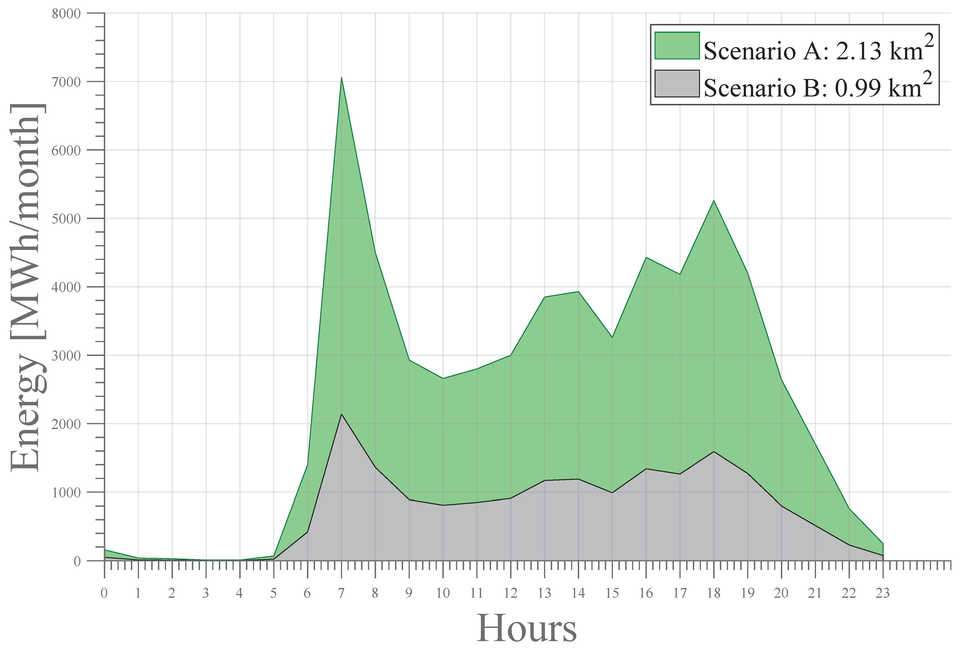Figure 12 shows the energy demand required by the charging infrastructure for electric vehicles in cases A and B studied. It is noticeable that as the service area increases, the energy needed to start up the infrastructure rises proportionally. Figure 12 follows the theoretical trend of the hourly distribution of vehicular traffic. As can be seen, there are at least four peaks of maximum demand at 07:00, 14:00, 16:00, and 18:00 h. During these hours, the vehicle density increases and thus increases the probability that an electric vehicle needs to charge the battery of the electric car.

The expected number of electric vehicles and the minimum total power required in the charging infrastructure is illustrated in Figure 13. The average number of charging terminals needed for each service station for cases A and B are 6 and 7, respectively. This slight difference responds to the geographical size of each scenario, i.e., the larger the coverage area with charging terminals for electric mobility, the greater the vehicle density and, consequently, the greater the probability that electric vehicle users will require charging their batteries. The ID of each station is represented in the x-axis of Figure 13. In addition, as the number of vehicles increases, the need for energy demand at each charging station increases. This is because more charging terminals will be needed to satisfy the demand for battery recharging in considerable waiting times to guarantee greater comfort to the users of the charging stations. The charging station with ID 4 has six charging terminals and requires an installed power of 297.71 MVA. The following equation was used to calculate the minimum number of charging stations required.

$$\begin{array}{c}ET=\frac{VT\ast CT}{PO}\hfill \end{array}$$

(32)

$ET$ is the number of charging terminals for electric vehicles, $VT$ is the vehicle traffic, $CT$ is the terminal charging time, and $PO$ is the charging station power output. For example, from Figure 13, we extract the information of the number of vehicles in case study A. Let us take as a reference a charging station with ID 4. The maximum number of electric vehicles traveling is approximately 600, then $frac$ 600 $Veh$ ∗ 0.5 h 50 kW = 6 by requiring at least six 50 kW charging stations $6\ast 50=300$ kW or $315.9$ kVA if 0.95 is considered to be power factor.

Therefore, the proposed model has demonstrated the ability to adapt to different case studies that allow us to analyze contingencies, which are very useful at the time of sizing because it will permit us to consider the electrical, civil, and logistical equipment to lead to the construction of adequately planned charge infrastructures.

5. Discussion

The relationship between the deployment of public and private charging stations with economic conditions and policy guidance presents itself as a complex challenge, as the adoption of electric vehicle charging technologies depends on a combination of factors, including tax incentives, vehicle acquisition costs, charging infrastructure, and policy guidance towards the energy transition. Government policies and regulations are essential in encouraging investment in charging infrastructure. Still, it is also vital to consider charging stations’ long-term profitability and financial sustainability, especially in the context of economic and political fluctuations. Therefore, an integrated approach involving key industry, political, and societal stakeholders is needed to achieve effective and sustainable deployment of EV charging stations worldwide.

The growing demand for electric vehicles is increasing research and development of more efficient batteries and faster and more accessible recharging technologies. However, it is necessary to remember that the mass adoption of electric vehicles poses complex technical and economic challenges that require coordinated and collaborative solutions from industry, governments, and society. It is essential to promote a transition to sustainable electric mobility in a strategic, planned, and sustainable manner over time to ensure an effective reduction in greenhouse gas emissions and a positive impact on air quality and public health.

6. Conclusions

This article has allowed us to plan ICSEC in geolocalized scenarios by considering actual transport variables at the trajectory level; they were supported by optimization algorithms such as Hungarian, multi-commodity flow problem, and graph theory.

The main contribution of this paper is its high potential to become a computational model and infrastructure manager for planning and resource allocation in electro-mobility. The heuristic has been demonstrated to be scalable. It has been validated through iterative processes that deal with contingency concepts to predict the maximum density of vehicular traffic in road networks.

The heuristic provides finite and scalable solutions over time. The hourly analysis of vehicle flow has permitted the identification of maximum and minimum demands experienced for each CS, which contributes to coordinating and managing battery-charging processes in electric vehicles. The criterion for CS sizing is based on empirical statistical techniques, which consider the average with two standard deviations.

The algorithm minimizes the travel route by solving the multiple-product problem with characteristic hourly mobility patterns under linear programming considerations. The solutions obtained are close to the optimal ones, because they are of NP-Complete complexity.

More global solutions to this combinatorial problem must be addressed, since their complexity increases exponentially as the topology grows. Finally, this article presents a novel approach to constructing and developing charge infrastructures in developing countries.

Future research will include the optimal topology study of charging stations to determine the optimal charging terminals to guarantee the hourly demand for EV charging. Moreover, power flows in EDS will be included to assess technically planned actions to satisfy the new electricity demand due to the high penetration of electric vehicles.