A Parameter-Free Method for Estimating the Stator Resistance of a Wound Rotor Synchronous Machine

Abstract

This paper presents a new online method based on low frequency signal injection to estimate the stator resistance of a Wound Rotor Synchronous Machine (WRSM). The proposed estimator provides a parameter-free method for estimating the stator resistance, in which there is no need to know the values of the parameters of the machine model, such as the stator and rotor inductances or the rotor flux linkage. In this method, a low frequency sinusoidal current is injected in the d axis of the stator current to produce a sinusoidal flux in the stator. In this paper, it is shown that the phase difference between the generated sinusoidal flux and the injected sinusoidal current is related to the stator resistance mismatch. Using this phase difference, the stator resistance is estimated. To validate the proposed model-free estimator, simulations were performed with Matlab Simulink and the results were compared with the extended Kalman filter observer. Finally, experimental tests, under different conditions, were performed to estimate the stator resistance of a WRSM.

1. Introduction

Synchronous machines are among the most popular types of electrical machines and are increasingly used in various applications. In recent years, many studies have been carried out on modeling, parameter identification, and control methods for this type of machine [1]. The parametric variation of machines with non-linear models is still an important drawback of automatic system controllers [2]. Most of the advanced control methods for synchronous machines are model-based and are dependent on the parameters of the machine. In particular, the stator resistance has a very important role in many advanced control methods such as Direct Torque Control (DTC) [2], Model Predictive Control (MPC) or sensorless control methods [3]. For example, in the DTC control method, a mismatch in the stator resistance value may introduce a considerable error in the estimated flux and electromagnetic torque, which can degrade the control performances.

Nevertheless, the stator resistance is not always equal to the value given by the manufacturer and it can change due to age, wear, temperature variations, etc. In addition, when the drive system is taken into account, the resistances of the driver and the interface wires are added to the equivalent stator resistance. Thus, for precise control, a stator resistance estimator is needed.

This paper presents a method for estimating the stator resistance without the need for information about the values of the motor parameters (such as d- and q-axis inductances). The proposed estimator is presented after a review of some existing estimation methods.

According to the scientific literature, the stator resistance estimation methods can be divided into three main categories:

• Direct measurement methods;
• Model-based estimation methods;
• Signal injection-based methods.

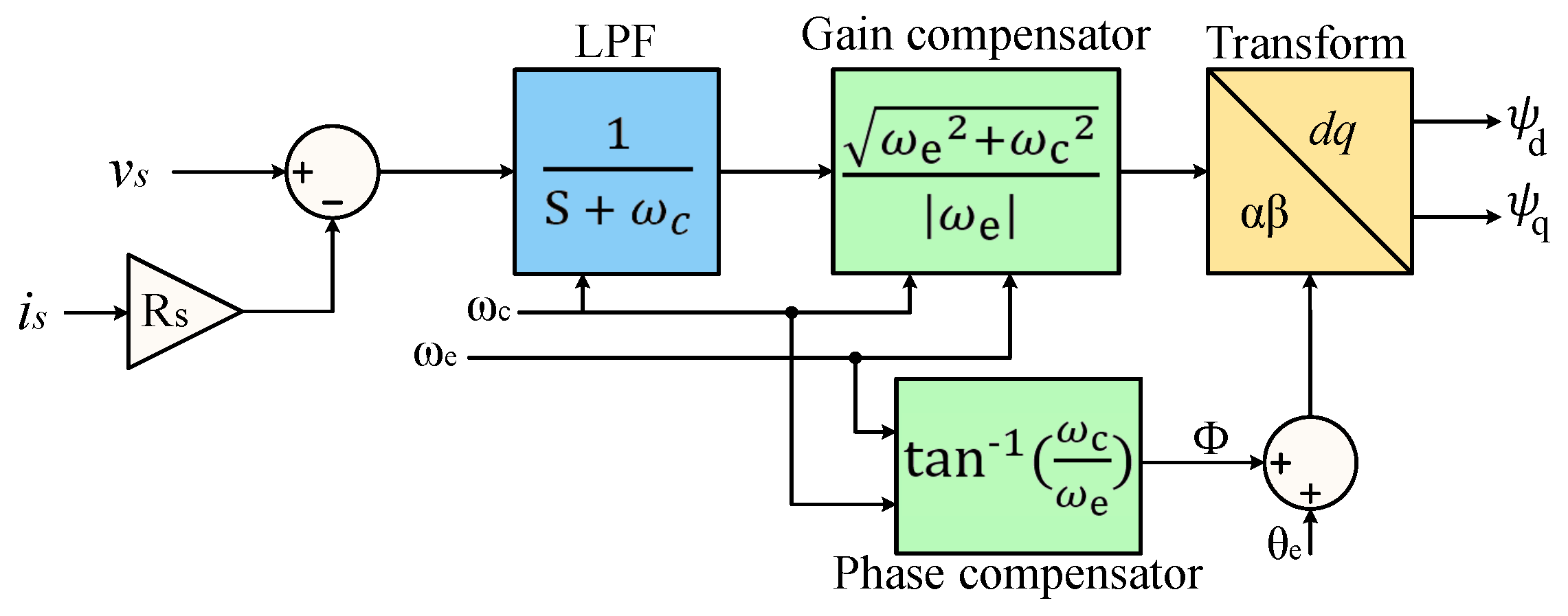
Direct measurement methods are usually realized under certain conditions, but due to temperature changes and the rest of the system influences, the resistance does not remain constant during the tests; therefore, they are not an accurate method. The model-based estimation methods are generally sensitive to variations in the motor parameters. Consequently, a precise estimation cannot be made if the parameters of the model are not available [4]. Among these methods, the Kalman filter observer [5,6,7] can be mentioned, which is robust towards measurement noises but requires a high amount of computational power due to the complex matrix operations. Other model-based online methods have also been presented in the literature that can estimate stator resistance and rotor speed simultaneously, such as full-order observers [8], reduced-order observers [9,10], and model reference adaptive observers [11,12,13,14,15,16,17]. The estimators based on a Model Reference Adaptive System (MRAS) compare a reference model (with measured variables) and an adjustable model (with estimated states) and according to the error between these two models, the desired variable is estimated. However, these methods are model-based and require the machine parameters to estimate the stator resistance. Another model reference adaptive estimator was also proposed in [18]. This method, unlike the classic model-based methods, does not require flux calculation, but the stator resistance estimation is performed individually only if the speed is available. A stator resistance estimator based on a fuzzy logic controller was also presented in [19] for an induction motor controlled by the DTC technique in which the resistance value is updated during operation. Cheng Luo et al. [20] also proposed a “phase-shift”-based method to compensate the stator resistance for motor drives. They decoupled the resistance estimator from the speed estimator by introducing a coefficient for operating point tracking compensation. In [21], a sensorless control of surface-mounted PMSM with online resistance estimation was proposed. This method uses a sliding mode observer to estimate the stator currents, and assuming the estimated current error is close to zero, a first-order low-pass filter is used to estimate the stator resistance. However, this method may not be precise when the initial resistance error is large [22].

The third category of stator resistance estimation methods is based on signal injection. There are some limited studies on DC signal injection [23,24,25], low-frequency signal injection [26], and high-frequency signal injection [27,28]. In [24], the authors presented a signal injection strategy to estimate the machine temperature through the stator resistance estimation of an induction motor. However, the estimator needs a look-up table for different current and temperature values to obtain the voltage drop in the semiconductors that is used in the algorithm. In [25], a DC-signal injection method was proposed. In this method, a DC signal is injected into the three-phase windings of the stator. Then, using a method that includes a high-pass digital filter, a low-pass digital filter, and a sample-and-hold function, the values of the dc components are obtained, and then the stator resistance is estimated. However, extracting the DC components is not easy since the magnitudes of the DC components are much smaller than the fundamental components and the frequency of the fundamental component depends on the rotor speed and hence on the operating point [29]. On the other hand, due to the current limitations of semiconductor devices, DC-signal injection methods cannot be directly applied to motors larger than 100 hp (75 kW) [23]. A low-frequency injection-based method for estimating the stator resistance for PMSMs was proposed in [26]; the method is based on injecting a three-level perturbation into $i_d$ and using two algorithms with different convergence speeds. However, this method is completely model-based and sensitive to the model parameters. Additionally, unstable convergence may occur in the saturation case [30]. High-frequency signal injection methods are mostly used for initial detection of rotor position [31,32] or estimation of the magnetization state [27], rather than for estimation of stator resistance. In these methods, some other problems such as the skin effect and the reactance values (which at high frequencies are more prominent than the resistance value) must be considered in the analysis [25].

In this paper, a new method based on low-frequency signal injection is proposed to estimate the stator resistance. The first advantage of this method is that it does not require machine parameters, which can be applied to the machines even with unknown parameters. Moreover, the variation of the different parameters does not affect the accuracy of the resistance estimation. The second advantage is the simplicity of the implementation, which does not require any complicated process. In the proposed method, a low-frequency sinusoidal current is injected into the d axis of the stator for a short time. This injected signal can produce a sinusoidal variation on the estimated flux of the q axis if there is a mismatch on the stator resistance value. The phase difference between the injected sinusoidal signal and the sinusoidal variation of the estimated flux is related to the initial value of the stator resistance, which allows to adjust and estimate the correct value of the stator resistance. The rest of the paper is structured as follows. The flux estimation is introduced in Section 2. In Section 3, the effect of stator resistance mismatch on the estimated flux is studied. The simulation and method explanation are presented in Section 4, and the experimental validations are provided in Section 5. Finally, Section 6 concludes this article.

2. Flux Estimation

With the method proposed in this paper, in order to estimate the stator resistance, the stator flux must first be estimated. In this study, a flux estimator, based on the voltage model, is used as introduced in [33,34]. In this method, the stator flux linkage can be calculated by integrating the back EMF of the stator windings. The stator voltage in the $\alpha \beta$ reference frame is described as (1):

$$v_s=R_s{i}_s+\frac{d{\psi }_s}{dt}$$

(1)

where $R_s$ is the stator resistance and $v_s$, $i_s$, and ${\psi }_s$ are the voltage, current, and stator flux, respectively. The stator flux can be expressed as follows:

$${\psi }_s=\int (v_s-R_s{i}_s)dt$$

(2)

The integration in (2) can cause a drift and saturation problems due to the initial condition or DC offset. To avoid this issue, a Low-Pass Filter (LPF) can be used instead of a pure integrator. Equation (3) describes the estimated flux in the Laplace transform, where ${\omega }_c$ is the cutoff frequency of the LPF in radians per second.

$${\psi }_s=\frac{(v_s-R_s{i}_s)}{s+{\omega }_c}$$

(3)

Using an LPF can solve the saturation and drift problems, but it can also add an error to the estimated flux. The gain and phase error produced by LPF can be described as (4) [33], where $Mag$ and $\phi$ represent the gain and the phase error, respectively, and ${\omega }_e$ is the synchronous angular frequency. It can be seen from (4) that there is a gain decrement and a phase delay due to the LPF.

$$\left\{\begin{array}{c}Mag=\frac{\left|{\omega }_e\right|}{\sqrt{{{\omega }_e}^2+{{\omega }_c}^2}}\hfill \\ \phi =\frac{\pi }{2}-{tan}^{-1}\left(\frac{{\omega }_e}{{\omega }_c}\right)\hfill \end{array}\right.$$

(4)

Choosing a cutoff frequency close to the operating frequency can decrease the DC offset of the estimated flux, but also introduces phase and magnitude errors. For example, when a cutoff frequency is chosen equal to the synchronous one (${\omega }_c={\omega }_e$), the ratio of the estimated flux to the actual flux has a magnitude of $\frac{1}{\sqrt{2}}$ with an angle of $\frac{\pi }{4}$. Thus, to reduce phase and magnitude errors, the cutoff frequency can be set as low as possible, but this will reduce the effectiveness of the low-pass filter in filtering out the DC offset that is likely present in the detected currents or voltages. Reference [34] suggests that the cutoff frequency be chosen as a fraction of the rotation frequency, as follows:

$${\omega }_c=\frac{\left|{\omega }_e\right|}{k}$$

(5)

where k is a constant. In this case, to prevent the time constant of the LPF from being much increased when the motor speed is close to zero, a lower limit must be considered for ${\omega }_c$. On the other hand, to eliminate the error produced by LPF, a gain and a phase compensator can be used as (6) [34]. This compensator is exactly the inverse of the error introduced in (4). Therefore, the selection of the gain and phase compensators is performed only using the ${\omega }_e$ and ${\omega }_c$.

$$\left\{\begin{array}{c}{G}_c=\frac{\sqrt{{{\omega }_e}^2+{{\omega }_c}^2}}{\left|{\omega }_e\right|}\hfill \\ {\phi }_c={tan}^{-1}\left(\frac{{\omega }_c}{{\omega }_e}\right)\hfill \end{array}\right.$$

(6)

Figure 1 illustrates the block diagram of the flux estimation method. In this method, after the integration of back EMF through an LPF, a gain and a phase compensator is used. Then, with a Park transformation, the stator fluxes in the $dq$ reference frame are obtained.

The stator flux estimator that is introduced depends on the stator resistance. In the next section, the effect of stator resistance mismatch on flux estimation is investigated.

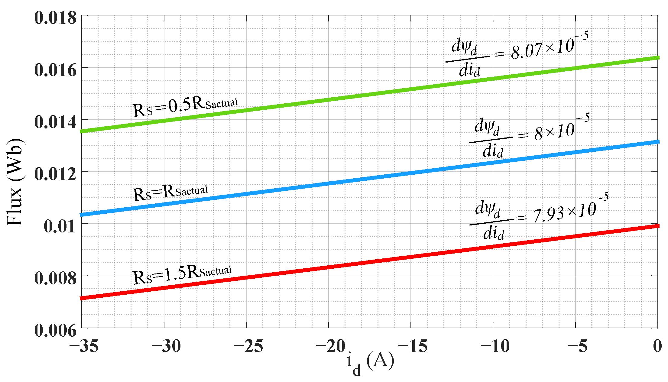
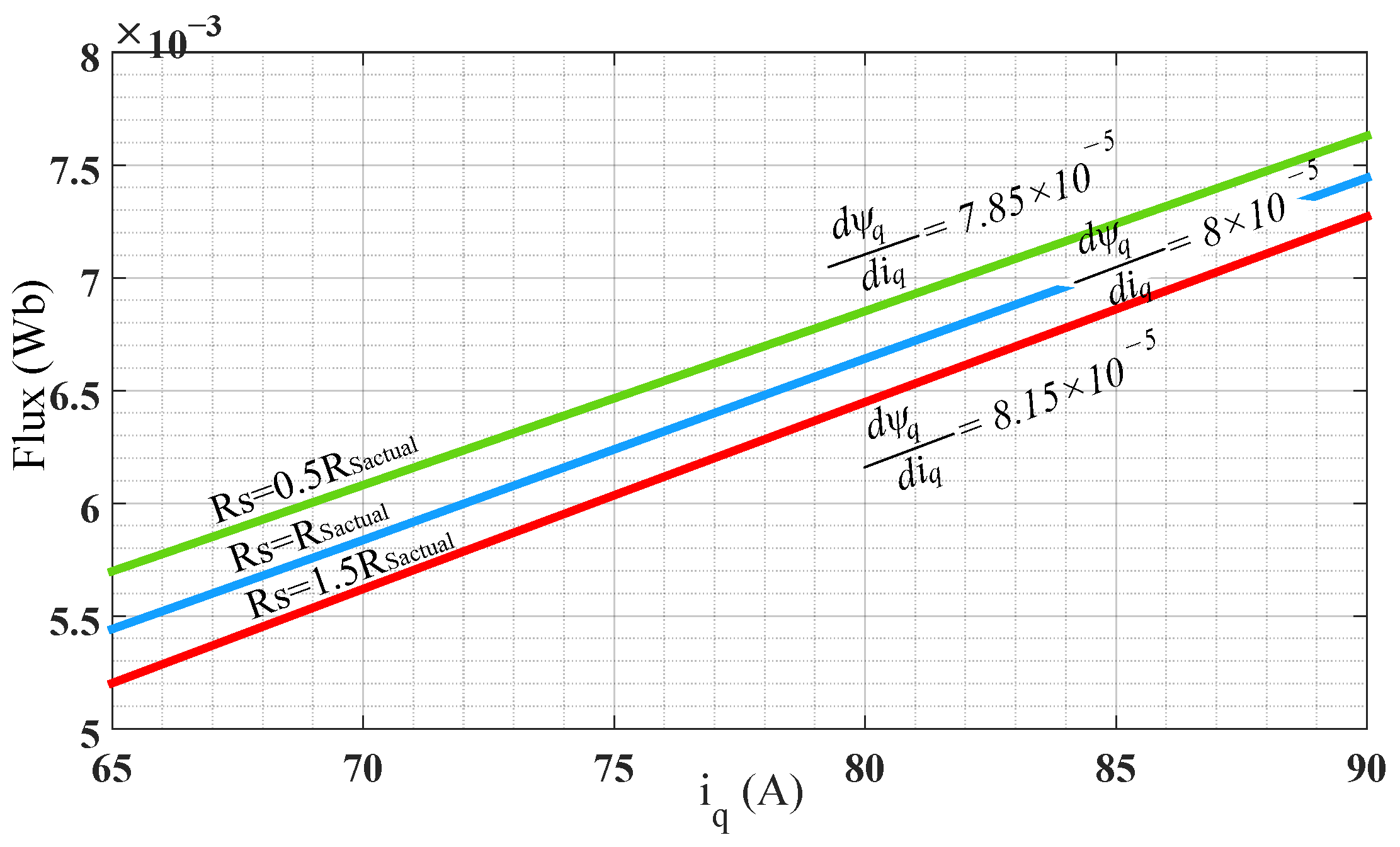
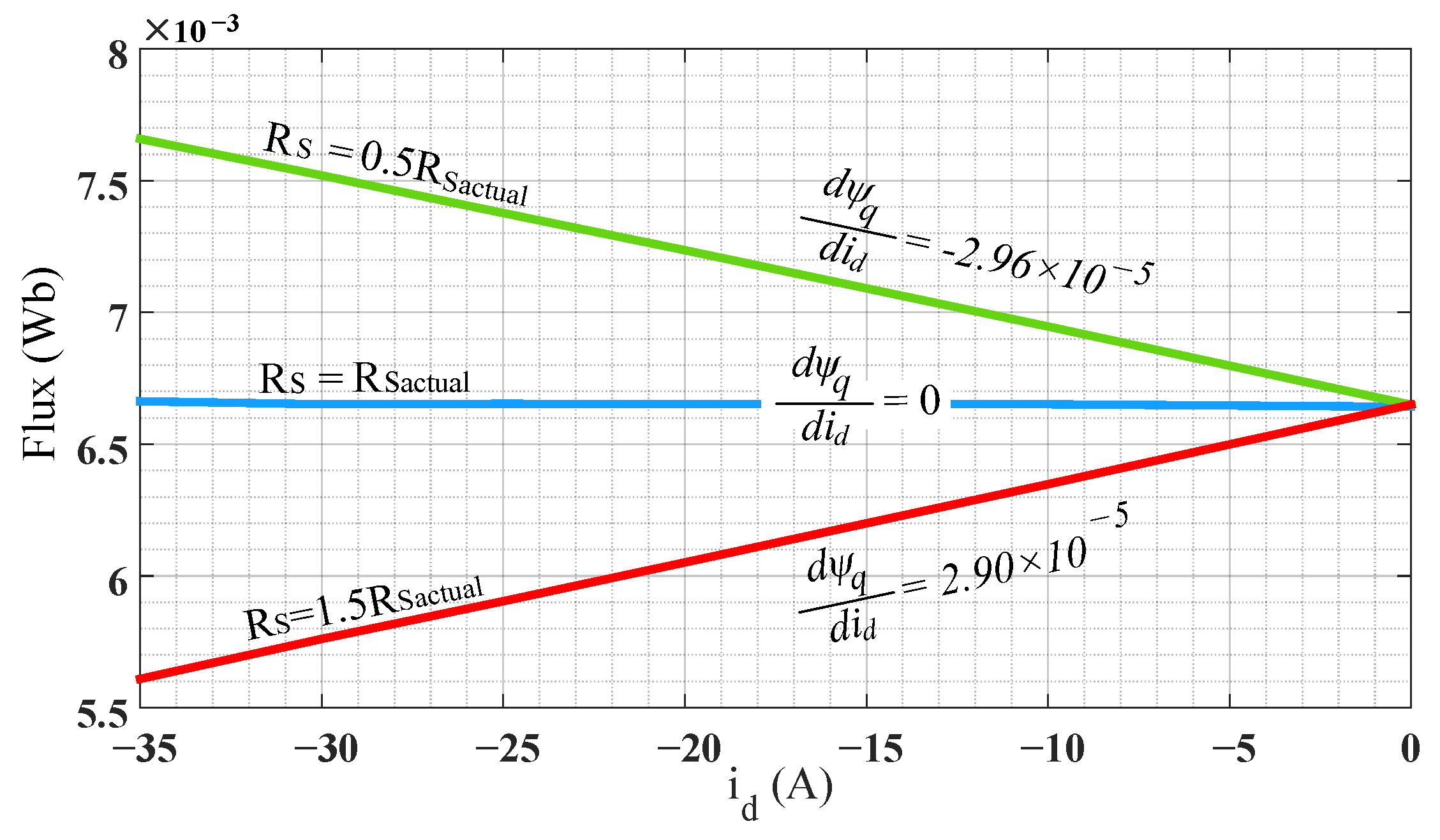
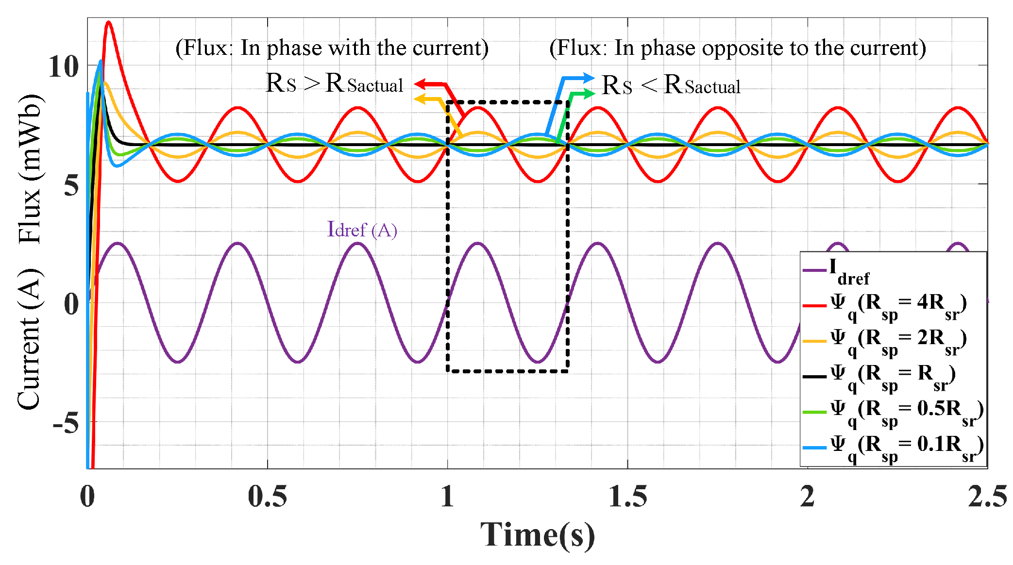
3. Effect of Stator Resistance Mismatch on the Estimated Flux

Since the presented flux estimator depends on the stator resistance, it is clear that an error in the stator resistance will cause an error in the estimated flux. By using the difference between the actual flux and the estimated one, the resistance error can be found. However, it is very difficult to measure the actual stator flux and therefore to know the error value of the estimated flux. Thus, in this paper, a method will be proposed to detect the error in the estimated flux without the need to measure the actual flux. Finally, using this error, the stator resistance mismatch will be detected.

In order to analyze the effect of stator resistance mismatch on the estimated flux, it is assumed that the compensator performs well, and the result is the same as with a pure integrator as seen in (2).

The resistance error is defines as (7):

$${\widehat{R}}_s=R_s+{\tilde{R}}_s$$

(7)

where $R_s$ is the actual resistance, ${\widehat{R}}_s$ is the initial resistance and ${\tilde{R}}_s$ is its error value. By substituting (7) in (2), the estimated flux is expressed as (8):

$${\widehat{\psi }}_s=\int (v_s-(R_s+{\tilde{R}}_s)i_s)dt={\psi }_s+\int -{\tilde{R}}_s{i}_{s}dt$$

(8)

where ${\psi }_s$ is the actual flux and the rest of the equation is the error part due to the resistance error; the tilde symbol represents the error part as (9).

$${\tilde{\psi }}_s=-{\tilde{R}}_s\int i_{s}dt$$

(9)

If the stator currents in the $\alpha \beta$ reference frame are considered sinusoidal as in (10):

$$\left\{\begin{array}{c}{i}_{\alpha }=I_{m}cos\left({\omega }_{e}t\right)\hfill \\ i_{\beta }=I_{m}sin\left({\omega }_{e}t\right)\hfill \end{array}\right.$$

(10)

by developing (9) and (10), the estimated flux error due to the resistance mismatch can be described as (11):

$$\left\{\begin{array}{c}{\tilde{\psi }}_{\alpha }=\frac{-{\tilde{R}}_s{I}_m}{{\omega }_e}sin\left({\omega }_{e}t\right)\hfill \\ {\tilde{\psi }}_{\beta }=\frac{{\tilde{R}}_s{I}_m}{{\omega }_e}cos\left({\omega }_{e}t\right)\hfill \end{array}\right.$$

(11)

By transforming (11) in the $dq$ reference frame, the estimated flux error can be expressed by (12), where ${\tilde{R}}_s$ is the error value of the stator resistance.

$$\left\{\begin{array}{c}{\tilde{\psi }}_d=\frac{-{\tilde{R}}_s{I}_q}{{\omega }_e}\hfill \\ {\tilde{\psi }}_q=\frac{{\tilde{R}}_s{I}_d}{{\omega }_e}\hfill \end{array}\right.$$

(12)

According to (12), the resistance mismatch can cause an error in the estimated flux. In the field weakening region ($i_q$ positive and $i_d$ negative), it can be noticed from (12) that a positive ${\tilde{R}}_s$ causes ${\tilde{\psi }}_d$ and ${\tilde{\psi }}_q$ to be negative and creates a negative offset in the estimated fluxes ${\widehat{\psi }}_d$ and ${\widehat{\psi }}_q$. Similarly, a negative ${\tilde{R}}_s$ makes ${\tilde{\psi }}_d$ and ${\tilde{\psi }}_q$ positive and therefore it causes a positive offset for the estimated fluxes ${\widehat{\psi }}_d$ and ${\widehat{\psi }}_q$. This behavior will also be observed in the simulation section.

Another consideration is the effect of stator resistance mismatch on the estimated flux profile in terms of currents. The effect of this mismatch on the flux gradient in terms of currents is shown in (13). In these relations, it is assumed that (${I_d}_1<{I_d}_2$ and ${I_q}_1<{I_q}_2$).

$$\left\{\begin{array}{c}\frac{\Delta {\tilde{\psi }}_d}{\Delta I_d}{|}_{I_q=cte}=\frac{{\tilde{R}}_s{I}_q(\frac{1}{{\omega }_{e1}}-\frac{1}{{\omega }_{e2}})}{I_{d2}-I_{d1}}\underset{{\omega }_{e1}>{\omega }_{e2}}{\to }sign\left(\frac{\Delta {\tilde{\psi }}_d}{\Delta I_d}\right)\propto -{\tilde{R}}_s\hfill \\ \frac{\Delta {\tilde{\psi }}_q}{\Delta I_q}{|}_{I_d=cte}=\frac{{\tilde{R}}_s{I}_d(\frac{1}{{\omega }_{e2}}-\frac{1}{{\omega }_{e1}})}{I_{q2}-I_{q1}}\underset{{\omega }_{e2}>{\omega }_{e1}}{\to }sign\left(\frac{\Delta {\tilde{\psi }}_q}{\Delta I_q}\right)\propto {\tilde{R}}_s\hfill \\ \frac{\Delta {\tilde{\psi }}_q}{\Delta I_d}|I_q=cte=\frac{{\tilde{R}}_s(\frac{I_{d2}}{{\omega }_{e2}}-\frac{I_{d1}}{{\omega }_{e1}})}{I_{d2}-I_{d1}}\underset{{\omega }_{e1}>{\omega }_{e2}}{\to }sign\left(\frac{\Delta {\tilde{\psi }}_q}{\Delta I_d}\right)\propto {\tilde{R}}_s\end{array}\right.$$

(13)

According to (13), it can be concluded that the slope of the estimated flux error in terms of $i_d$, or the value of $\left(\frac{\Delta {\tilde{\psi }}_d}{\Delta I_d}\right)$, has the opposite sign to the error value of the stator resistance ($-{\tilde{R}}_s$). It means that if the estimated resistance is lower than the actual resistance (${\widehat{R}}_s<R_s$), the resistance error value (${\tilde{R}}_s$) is negative, and the value of $\left(\frac{\Delta {\tilde{\psi }}_d}{\Delta I_d}\right)$ is positive; therefore, with a positive error, the value of the estimated flux in terms of $i_d$ or $\left(\frac{\Delta {\widehat{\psi }}_d}{\Delta I_d}\right)$ is more than the real one. It can also be said that for positive values of ${\tilde{R}}_s$, the value of $\left(\frac{\Delta {\widehat{\psi }}_d}{\Delta I_d}\right)$ is lower than the real one. This argument is also valid for the values of $\left(\frac{\Delta {\widehat{\psi }}_q}{\Delta I_q}\right)$ and $\left(\frac{\Delta {\widehat{\psi }}_q}{\Delta I_d}\right)$, which have the same sign as the error value of the stator resistance (${\tilde{R}}_s$). However, in this study, we only use the third row of (13), as explained below.

The crucial point in this section is that, in the constant current of $i_q$, it is expected that ${\psi }_q$ does not depend on the current $i_d$, and thus the value of $\left(\frac{\Delta {\widehat{\psi }}_q}{\Delta I_d}\right)$ is expected to be equal to zero. However, according to (13), this value has the same sign as the error value of the stator resistance. This means that for ${\tilde{R}}_s>0$, the value of $\left(\frac{\Delta {\tilde{\psi }}_q}{\Delta I_d}\right)$ is positive, so the value of $\left(\frac{\Delta {\widehat{\psi }}_q}{\Delta I_d}\right)$ is greater than zero and positive, and for ${\tilde{R}}_s<0$, the value of $\left(\frac{\Delta {\tilde{\psi }}_q}{\Delta I_d}\right)$ and therefore $\left(\frac{\Delta {\widehat{\psi }}_q}{\Delta I_d}\right)$ is less than zero or negative. Therefore, by observing the sign of $\left(\frac{\Delta {\widehat{\psi }}_q}{\Delta I_d}\right)$, the sign of ${\tilde{R}}_s$ can be found. From this, it is possible to determine if ${\widehat{R}}_s$ is greater or less than the actual resistance of the motor. In this paper, this behavior is used to estimate the stator resistance.

Before explaining the estimation algorithm in the simulation section, the effect of stator resistance mismatch on the estimated flux will be observed.

4. Simulation and Method Explanation

To investigate the performances of the flux estimator and the effect of stator resistance mismatch, simulations were conducted for a WRSM with MATLAB Simulink. The WRSM studied is a low-voltage and high-current motor for automotive applications powered by a three-phase inverter and a 12-volt DC battery. The rotor also has a separate power supply that allows a higher degree of freedom for the control system. An input filter with a large capacitor is used to protect the battery from instantaneous currents and voltage peaks. Figure 2 shows a schematic of this system, where the control card consists of a vector control with PI regulators for $i_d$ and $i_q$. The parameters of the simulated model also are listed in

Table 1. Simulation parameters.

Parameter	Symbol	Value
Stator resistance	$R_s$	20 m$\mathrm{\Omega }$
d-axis inductance	$L_d$	80 $\mathsf{\mu }$H
q-axis inductance	$L_q$	80 $\mathsf{\mu }$H
Mutual inductance between rotor and stator	M	3 mH
Number of pole pairs	$N_p$	6

.

4.1. Estimated Flux

In these simulations, the method introduced in Figure 1 was applied to estimate the stator flux. The constant k in (5) was chosen as $k=4$, and the lower limit of ${\omega }_c$ was considered equal to 1 for speeds close to zero, in order to avoid that the LPF time constant increases too much. In the first simulation, in a constant $i_q$, the estimated flux ${\widehat{\psi }}_d$ was obtained as a function of the current $i_d$, and in a constant $i_d$, the estimated ${\widehat{\psi }}_q$ was obtained in terms of $i_q$. Figure 3 and Figure 4 show the estimated fluxes ${\widehat{\psi }}_d$ and ${\widehat{\psi }}_q$, respectively, in three different cases: the blue one where the stator resistance is error-free, the red one where the initial resistance (or the resistance used in the flux estimator) is $50\%$ higher than the actual value, and the green one where the initial resistance is $50\%$ lower than the actual value. Figure 4 illustrates the estimated flux ${\widehat{\psi }}_q$ in terms of $i_q$. As discussed before, the stator resistance error can cause an offset and a change in the slope. As can be noticed in these figures, an error in the resistance value induces an error in the estimated flux. As discussed in the previous section, when the initial resistance is less than the actual value, the estimated flux has a positive offset, and when the initial resistance is greater than the actual value, the estimated flux has a negative offset. Additionally, as expected from (13), the slope of the diagrams could also contain an error.

Figure 5 demonstrates the estimated flux ${\widehat{\psi }}_q$ in terms of $i_d$. According to this figure, for an initial resistance lower than the actual value, the slope of this diagram is negative, and for a resistance higher than the actual value, the slope is positive. For the error-free case this value is equal to zero; in other words the flux ${\widehat{\psi }}_q$ does not depend on the current $i_d$, which confirms the results obtained in Equation (13).

From the estimated flux ${\widehat{\psi }}_q$ in terms of $i_d$, the error in the stator resistance can be detected. In another simulation, the flux ${\widehat{\psi }}_q$ is estimated by applying a sinusoidal current at $i_d$ for different values of ${\widehat{R}}_s$. Figure 6 illustrates the estimated flux ${\widehat{\psi }}_q$ while $i_q$ is constant, and there is a sinusoidal current injected into $i_d$, for different values of ${\tilde{R}}_s$. As shown in this figure, when the value of ${\widehat{R}}_s$ is bigger than the actual value, the estimated flux is in phase with $i_d$, which means that when $i_d$ increases, the flux ${\widehat{\psi }}_q$ also increases, and when $i_d$ decreases, the estimated flux ${\widehat{\psi }}_q$ also decreases. In the cases where the stator resistance is smaller than the actual value, it is observed that the flux ${\widehat{\psi }}_q$ changes by 180 degrees of phase shift concerning $i_d$. In other words, the flux ${\widehat{\psi }}_q$ decreases with the increase in $i_d$, and it increases with the decrease in $i_d$. When the resistance is error-free, as expected, the flux ${\widehat{\psi }}_q$ does not depend on $i_d$, and despite the sinusoidal changes in $i_d$, the flux ${\widehat{\psi }}_q$ is constant.

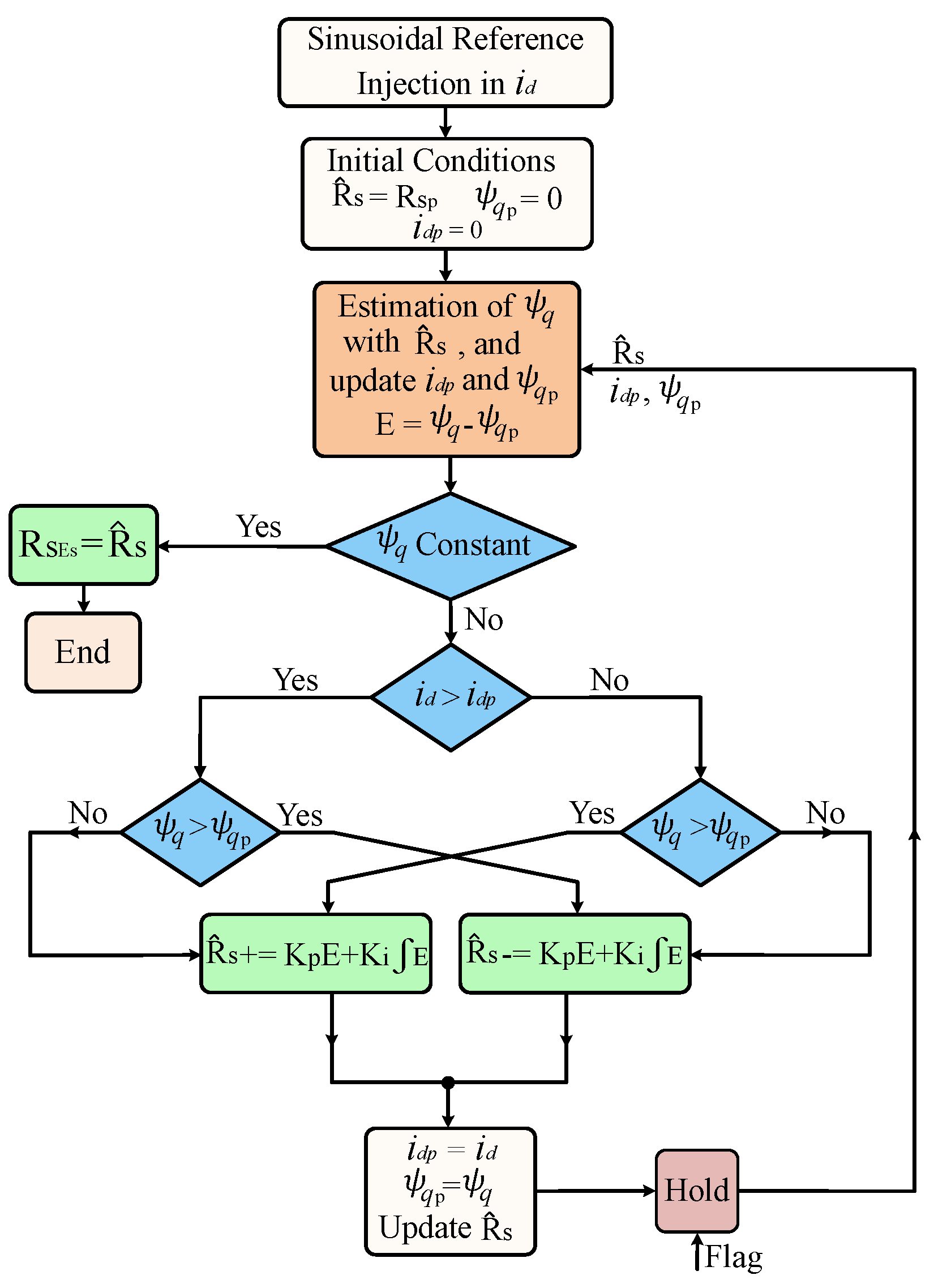
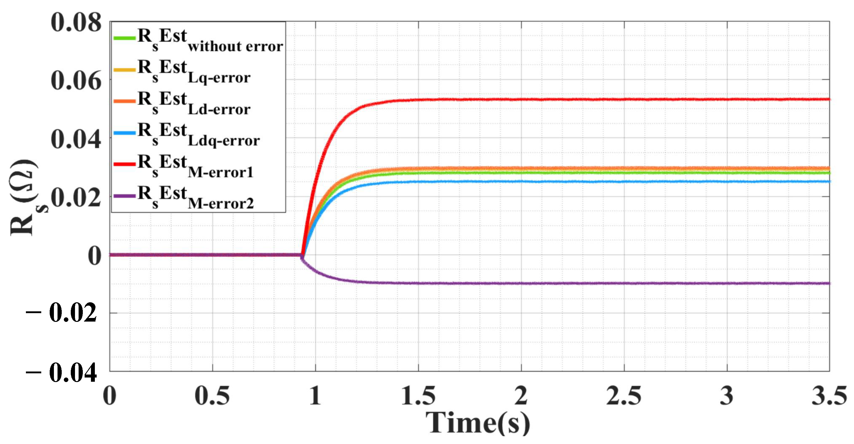
4.2. Estimation of Stator Resistance

In the previous subsection, it has been shown that in the case of a stator resistance error, the estimated flux ${\widehat{\psi }}_q$ varies as a function of $i_d$. Therefore, by observing the estimated flux ${\widehat{\psi }}_q$ in terms of $i_d$, the stator resistance can be adjusted. The flowchart in Figure 7 displays the resistance estimation algorithm.

According to this flowchart, a sinusoidal signal is first applied to the d-axis current of the stator ($i_d$). Then, with the initial value of the stator resistance, the flux ${\widehat{\psi }}_q$ is estimated. If the estimated flux ${\widehat{\psi }}_q$ changes in proportion to $i_d$, the estimated resistance must be reduced. If ${\widehat{\psi }}_q$ changes in opposite to $i_d$, the estimated resistance must be increased. The frequency of the iteration of this process is determined by the input flag that is explained later, and the process continues until the flux ${\widehat{\psi }}_q$ no longer changes with changes in $i_d$.

To implement the proposed algorithm, it is required to choose the frequencies of the injected sinusoidal signal ($f_{sin}$) and the iteration time of the calculation block (or the sampling time). The selection of the frequency of the injected signal depends on the flux estimation rate. This frequency is limited by the LPF used to estimate the flux, and must be lower than the cutoff frequency of the LPF (${\omega }_c$) to ensure that the estimated flux is not affected by a drop in amplitude or a shift in phase. Selecting a sinusoidal signal frequency higher than the cutoff frequency of the filter may result in incorrect convergence of the estimator. To choose the sampling time, it should be considered that an acceptable number of samples are taken in a sinusoidal period, so a sampling time can be chosen to guarantee that $T_s<\frac{1}{20}{T}_{sin}$. The following simulations were performed at $i_d=0$, $i_q=90$ A, and the rotor speed of 680 rpm. Considering the number of pole pairs $N_p=6$, the electrical rotation frequency was equal to ${\omega }_e=136$$\pi$(rad.s${}^{-1})$, and with $k=4$, ${\omega }_c=34$$\pi$(rad.s${}^{-1})$. The sinusoidal injected signal was selected as $i_{dref}=2.5$ sin$(16 \pi )$, where $f_{sin}=16$$\pi$(rad.s${}^{-1})$ was chosen to be less than 0.5 ${\omega }_c$. The amplitude also was chosen as 2.5 A, about $2\%$ of the nominal current. In general, as the amplitude of the injected sinusoidal signal increases, the amplitude of the changes in the estimated flux increases, which can increase the rate of resistance estimation. However, a high current amplitude causes more losses. Choosing an amplitude of about $2–5\%$ of the nominal current can lead to an acceptable estimation rate and also having few losses. The sampling frequency was also chosen to be equal to $T_s=5$ ms about $\frac{1}{25}{T}_{sin}$. At each sampling, a flag is sent to the calculating block that leads the algorithm to an iteration. Figure 8 summarizes the stator resistance estimation scheme of the proposed algorithm.

Next, to observe the performance of the stator resistance estimator, other simulations were conducted for a WRSM in Matlab Simulink. In the first simulation, we set $i_{qref}=90$ A and $i_{dref}=2.5sin(16 \pi )$, and the initial value of the stator resistance was chosen as $R_{sp}=0.2\mathrm{\Omega }$, which is 10 times greater than its actual value. Figure 9 shows the current $i_d$, the estimated flux ${\widehat{\psi }}_q$, and the estimated resistance ${\widehat{R}}_s$. The estimation method was applied at $t=3$ s until $t=5$ s, when the resistance was estimated. At $t=6$ s the real value of the resistance was changed to $R_s=0.04\mathrm{\Omega }$ and at $t=7$ s the estimator was run again and the estimated resistance value converged towards the new resistance value. As can be seen, the value of the stator resistance, despite a large error in the initial value, was correctly estimated in a fall time of $t_f$ = 0.375 s.

Figure 10 also shows the estimation of stator resistance when the initial value was $R_{sp}=0.002\mathrm{\Omega }$, which is 10 times less than its actual value. In this figure it can be seen that the estimation of the stator resistance behaves as expected.

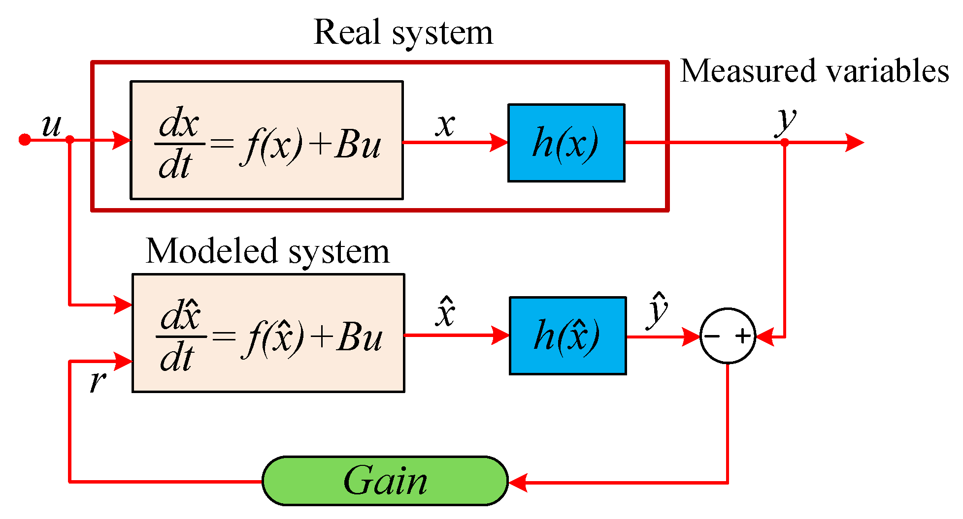
4.3. Kalman Filter Estimator

In this section, a comparison is made between the proposed estimator and the Kalman filter estimator. The Kalman filter is a mathematical model that runs in parallel to the actual system and provides the estimation of the states of linear systems [35]. Figure 11 shows the structure of an Extended Kalman Filter (EKF) observing the states of an actual system.

Using the system model of a WRSM, the state equations for the estimator can be presented as follows:

$$\left\{\begin{array}{c}\frac{d{i}_d}{dt}=\frac{v_d}{L_d}-\frac{{\widehat{R}}_s}{L_d}{i}_d+\frac{{\omega }_e{L}_q}{L_d}{i}_q\hfill \\ \frac{d{i}_q}{dt}=\frac{v_q}{L_q}-\frac{{\widehat{R}}_s}{L_q}{i}_q-\frac{{\omega }_e}{L_q}(L_d{i}_d+M{i}_e)\hfill \\ \frac{d{\widehat{R}}_s}{dt}=0\hfill \end{array}\right.$$

(14)

where $v_d$ and $v_q$ are the voltages in the $dq$ axes, $i_e$ is the rotor excitation current, and ${\omega }_e$ is the synchronous angular frequency. In addition, $L_d$ and $L_q$ are the stator inductance on the d and q axes, respectively, and M is the mutual inductance between the rotor and the stator. This simulation was performed at a constant current of $i_q=80$ A and $i_d=-10$ A. The currents $i_d$ and $i_q$ estimated by the Kalman observer as well as the measured currents can be seen in Figure 12.

The estimated resistance is also shown in Figure 13. It is observed that the Kalman observer is able to correctly estimate the stator resistance in a short time (less than 0.5 ms).

However, the Kalman observer has two main drawbacks: The first problem is a high computational load, and the second one, like the other model-based observers, is that it depends on the model parameters. To estimate the stator resistance, the values of the motor parameters such as $L_d$, $L_q$, and M need to be specified in the EKF design, while with the proposed method, those parameters are not needed. In model-based observers, an error in each parameter leads to an error in the estimated parameter. To observe the effect of motor parameters error on estimated resistance, the motor parameters are given to the Kalman observer with some errors. Figure 14 illustrates the estimated resistance while there are errors in the other parameters.

In Figure 14, it can be seen that if only $L_d$ or $L_q$ have a $50\%$ error, the resistance value of $R_s$ is estimated with errors of $8.5\%$ and $15\%$, respectively. If both $L_d$ and $L_q$ have a $50\%$ error, the error is greater (about $50\%$). This error increases when the mutual inductance M has an error, because as can be seen in Table 1, its value is much higher than the $dq$ inductances. In this figure the red diagram shows the estimated resistance while M is $50\%$ lower than the actual value, and the purple diagram shows the estimated resistance while M is $50\%$ greater than the actual value, at which the errors correspond to $50\%$ and $150\%$, respectively. These results show that despite the high speed of the Kalman estimator to estimate the stator resistance, if the other parameters of the model contain an error, the estimated resistance will also have an error that can be significant in certain cases, as can be seen in Figure 14.

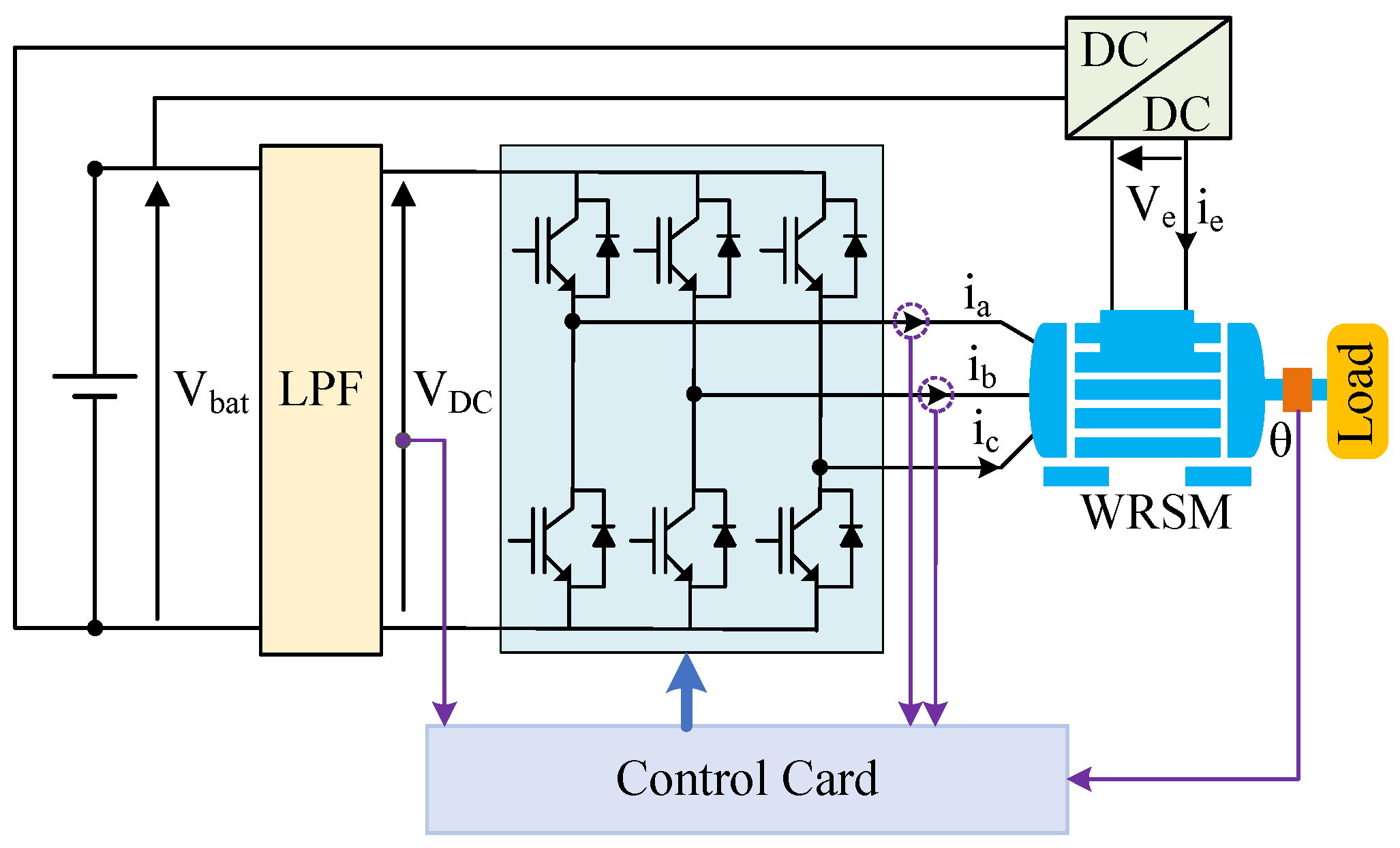
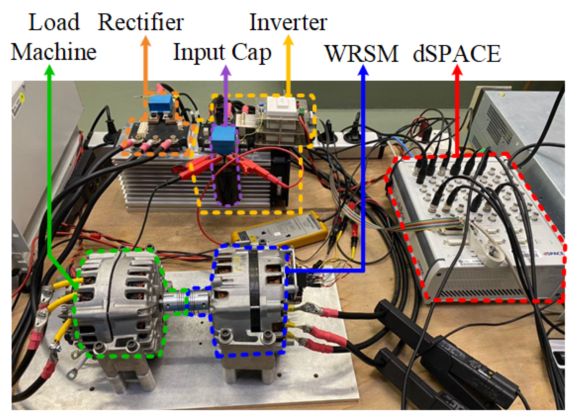
5. Experimental Results

In order to verify the proposed estimator, experimental tests were carried out on a WRSM. The prototype platform is shown in Figure 15. The WRSM under study was designed by Valeo for mild-hybrid applications for the automotive industry with 12 V rated voltage, 1.5 kW rated power, and a rotor excitation current of up to 8 A. The experimental setup consisted of two WRSMs; the first machine was controlled and its stator resistance was estimated, and the other was used as a load for the first machine. A dSPACE MicroLabBox was used to control the system and it sent the switching signals to a three-phase inverter with a frequency of 10 kHz. A 12 volt DC power supply was used as the input source of the inverter to emulate a car battery. The rotor excitation winding was also powered by a controllable DC voltage source.

5.1. Flux Estimation

In the first test, the effect of a resistance mismatch on the estimated flux was studied. To do so, with a current reference of $i_q=$ 35 A, a sinusoidal current was applied to $i_d$ and the flux ${\widehat{\psi }}_q$ was estimated.

In this test, a sinusoidal current was applied to $i_d$ and the flux ${\widehat{\psi }}_q$ was estimated while the value of the stator resistance in the equations of the flux estimator was first set to a value $50\%$ lower than its actual value; then, it was set as equal to its real value, and then it was fixed to a value $50\%$ higher than its real value.

Figure 16 shows the current $i_d$ and the estimated flux ${\widehat{\psi }}_q$. In this figure, as in the simulation results, it can be observed that at the beginning, when the set value of $R_s$ to be lower than its real value, the current $i_d$ and the flux ${\widehat{\psi }}_q$ had a phase difference of 180 degrees, so the flux ${\widehat{\psi }}_q$ decreased when $i_d$ increased and it increases when $i_d$ decreased. Then, when the fixed value of $R_s$ was equal to its real value, ${\widehat{\psi }}_q$ was almost constant and stable. Finally, when the set value of the resistance was greater than its real value, the current $i_d$ and the flux ${\widehat{\psi }}_q$ were in phase.

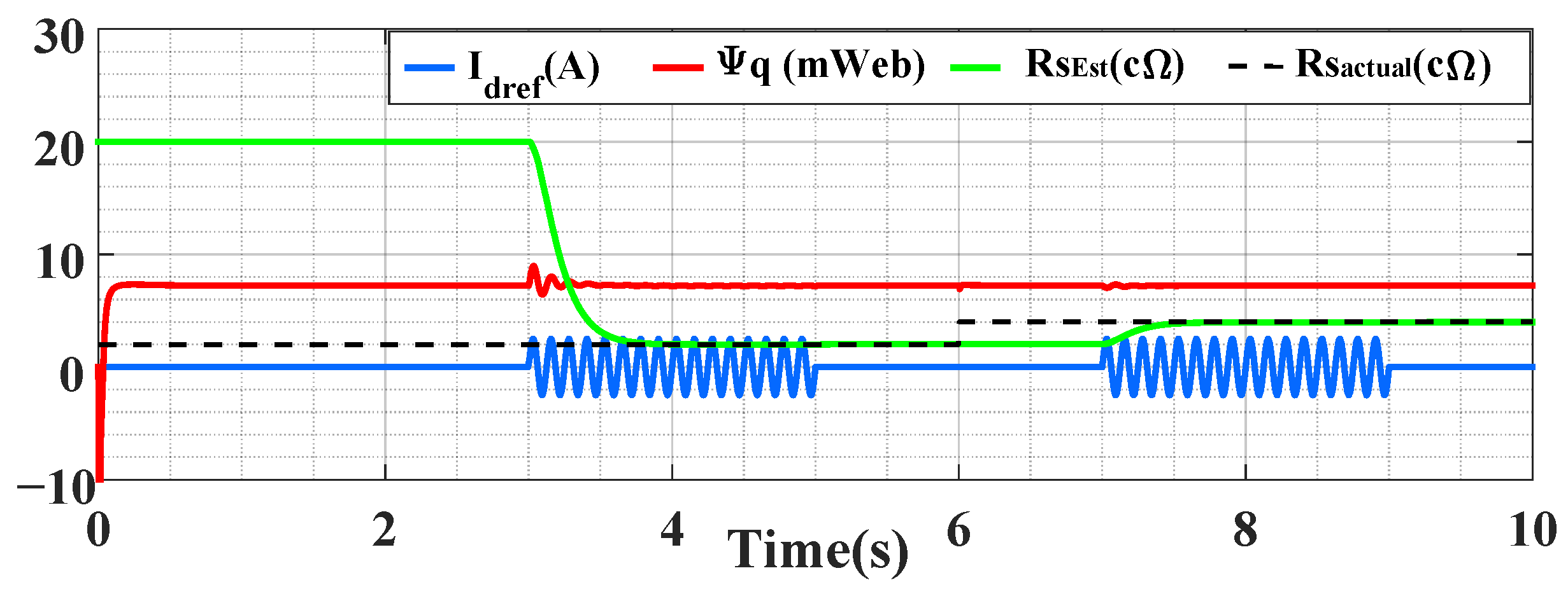
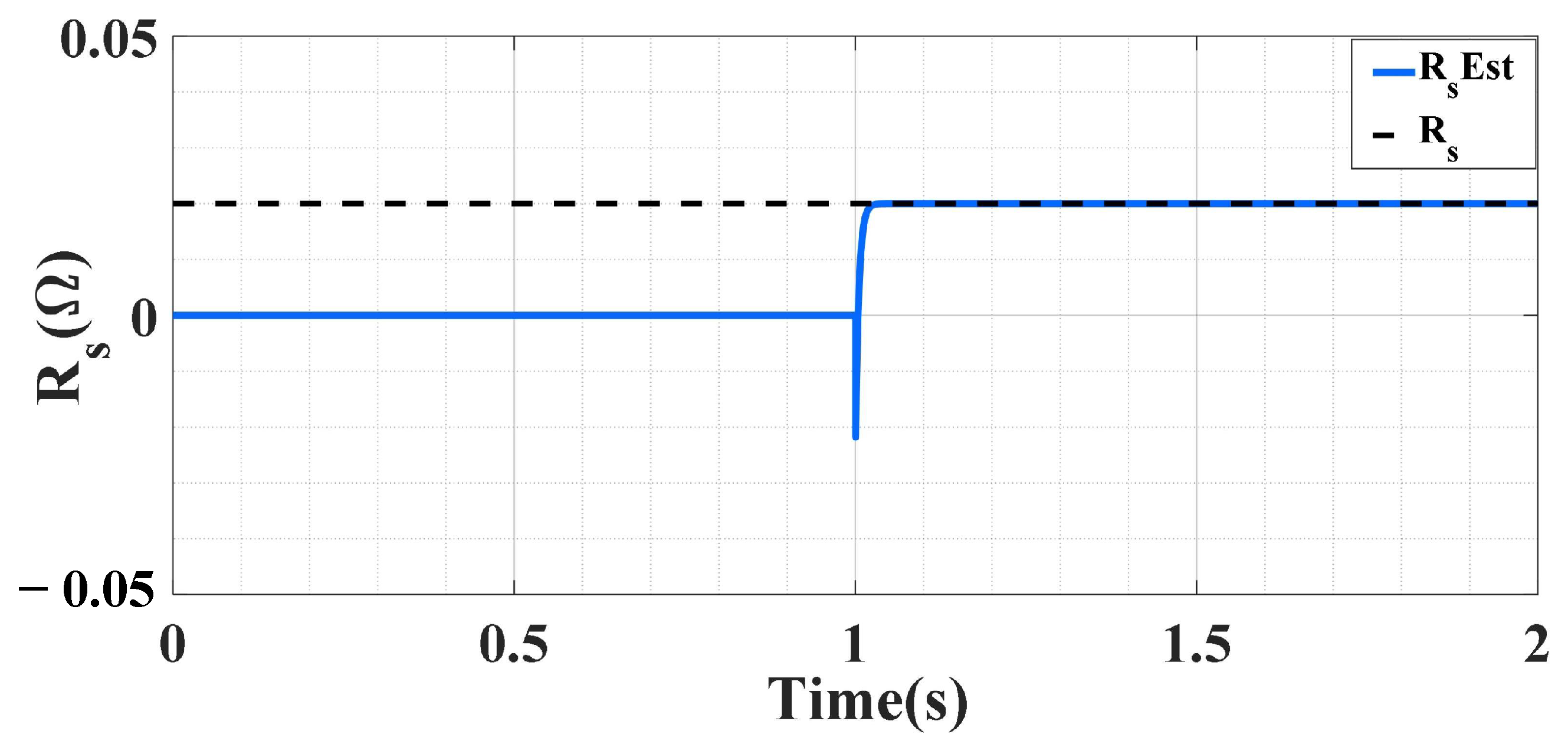
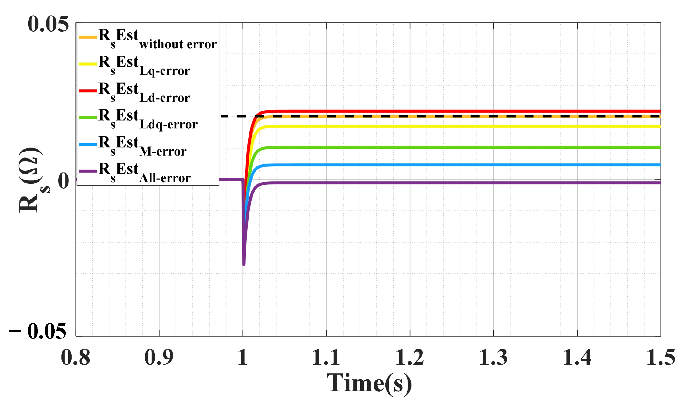
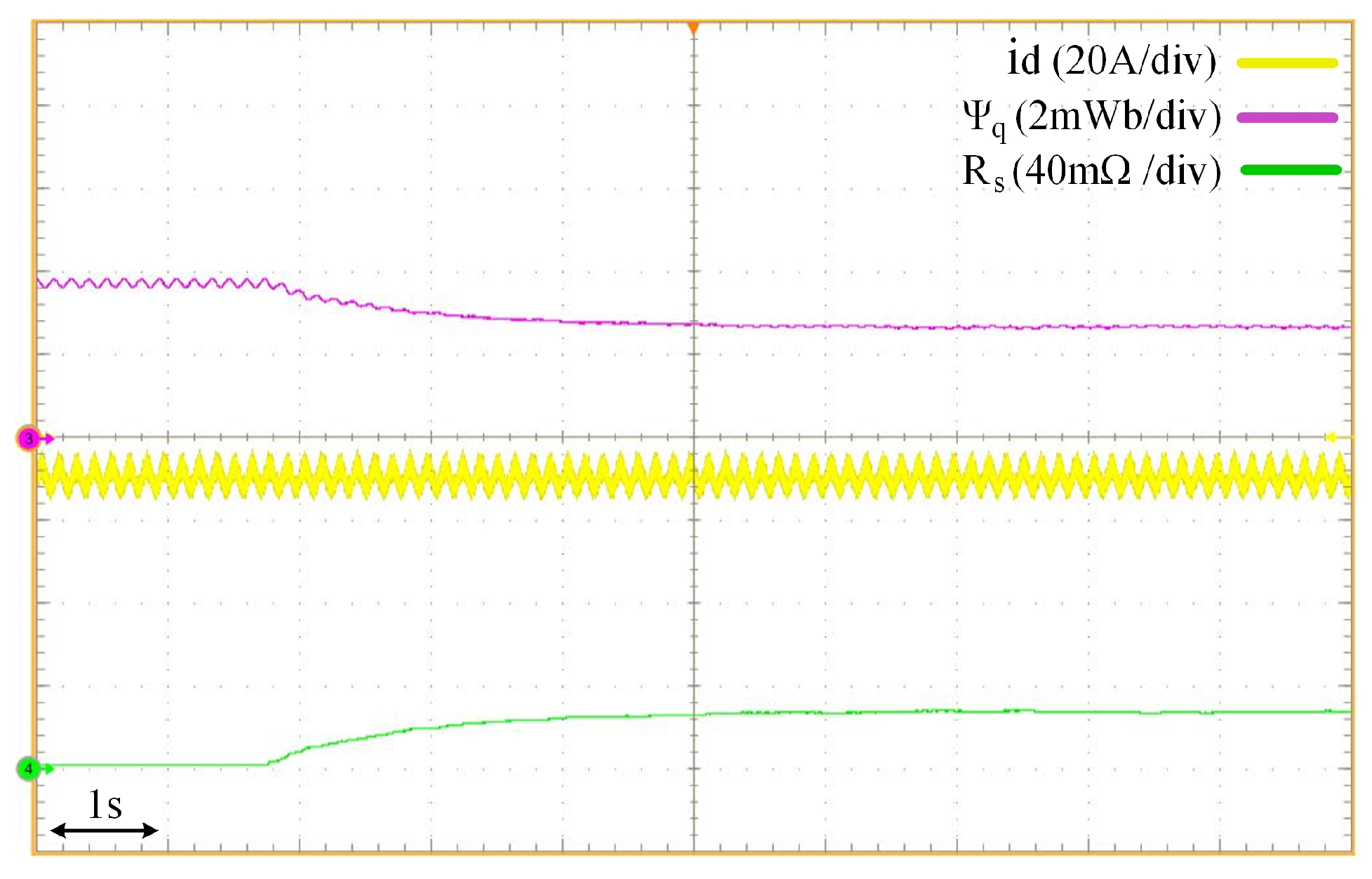
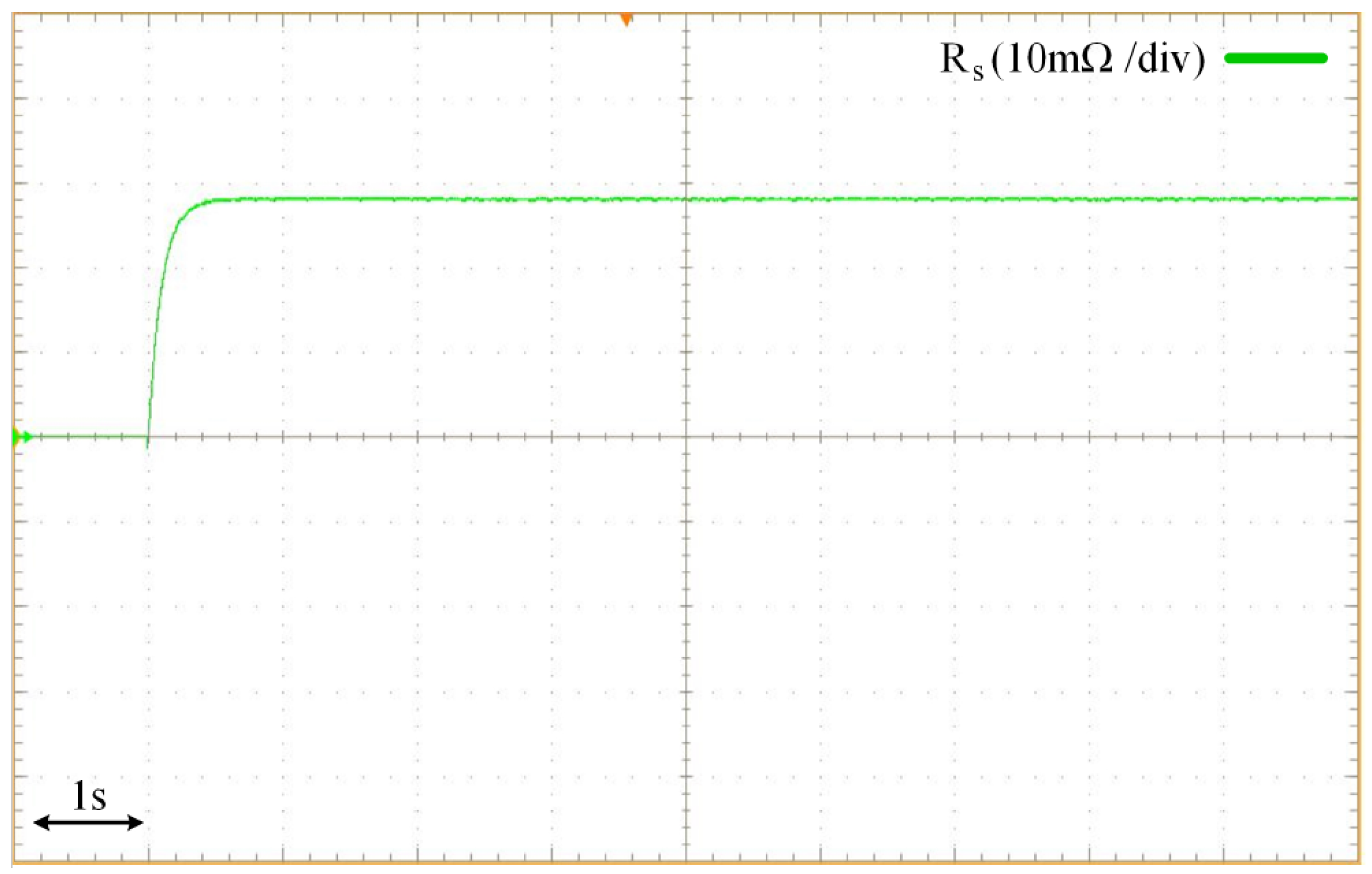
5.2. Stator Resistance Estimation

In the next test the resistance estimation algorithm was implemented. In this experiment, $i_q=35$ A, and for the sinusoidal signal injected into $i_d$, the frequency of the sinusoidal wave was $16\pi$ (rad.s${}^{-1})$ and the amplitude was equal to 5 A (about $4\%$ of the nominal current). In the first test the initial resistance value was considered as 2 m$\mathrm{\Omega }$. The sinusoidal signal was injected into $i_d$, and the estimation algorithm was executed. Figure 17 illustrates the result of this estimation. As shown in Figure 17, the estimated flux first oscillated sinusoidally with a phase shift of 180 degrees with $i_d$. Then, by starting the resistance estimation algorithm, the amplitude of the estimated flux oscillation was decreased and the estimated resistance converged towards 27.2 m$\mathrm{\Omega }$.

This experiment was repeated under the same conditions, but this time the initial value of the stator resistance was chosen as 200 m$\mathrm{\Omega }$. The result of this estimation is also illustrated in Figure 18. As is seen, first the estimated flux had oscillations in phase with $i_d$. Then, after starting the estimation, the oscillation in the estimated flux was reduced, and the estimated resistance converged to 27.2 m$\mathrm{\Omega }$.

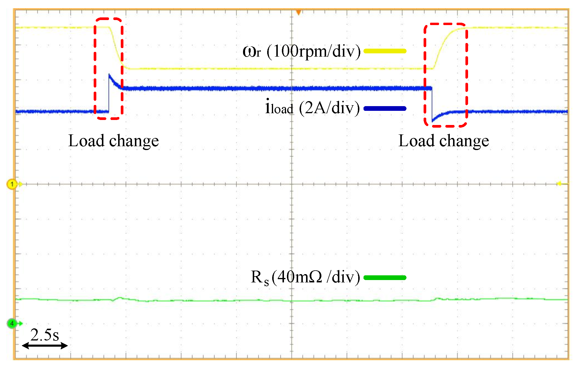
5.3. The Effect of a Sudden Change in Load

To investigate how the estimator responds to a sudden change in load level and shaft speed, another experiment was performed. In this test, the motor currents ($i_d$ and $i_q$) were kept constant and the rotor speed varied with the output load. As mentioned earlier, a second machine was connected to the studied machine as an output load. The second machine worked as a generator and supplied a resistive load. In this test, to make a sudden change in the motor load, the resistive load connected to the generator suddenly changed. Figure 19 shows the stator resistance estimation during the load changes. In this figure, it can be observed that after a sudden change in output load, the estimated resistance remained stable.

5.4. Estimation of Resistance by Kalman Observer

Next, to compare and validate the proposed estimator, a Kalman filter observer was applied to estimate the stator resistance. In this test, the stator currents were equal to $i_d=0$ and $i_q=35$. Figure 20 illustrates the resistance estimated with the Kalman observer, which converged to 28 m$\mathrm{\Omega }$. Figure 21 also shows the estimated resistance in the case of an error in the motor parameters. It can be seen that as in the simulation part, for the error of $50\%$ on $L_d$ or $L_q$, the estimated resistance faced a small error ($5.7\%$). This error increased with a mismatch in the mutual inductance M. The red diagram in this figure shows the estimated resistance while M was about $50\%$ lower than the actual value (which led to an error of $89\%$ in the estimated resistance), and the purple diagram shows the estimated resistance while M was about $50\%$ bigger than the actual value (which caused an error of $135\%$ in the estimated resistance). The results observed in this section demonstrate the sensitivity of model-based estimators, and it was observed that in this type of estimators, an error in one of the model parameters can lead to a significant error in the estimated parameter. However, the proposed estimator is completely independent of the model parameters.

6. Conclusions

In this paper, a new method based on low frequency signal injection has been proposed to estimate stator resistance. This technique is based on the phase difference between the injected sinusoidal current and the estimated flux variations. In this method, a low frequency sinusoidal current is injected into the d axis of the stator and during this time the stator flux is estimated. It was shown that by injecting a low-frequency sinusoidal signal into the stator d-axis, in case of stator resistance mismatch, the estimated flux of the q-axis gets sinusoidal variation, and the phase difference between the injected sinusoidal signal and the sinusoidal variation of the estimated flux is related to the value of estimated stator resistance. This phase difference was used to adjust the stator resistance. The proposed method provides a simple, parameter-free technique for estimating stator resistance without the need for the parameters of the machine model, such as stator and rotor inductances or the rotor flux linkage.

The simulation work, first, showed the effect of a stator resistance mismatch on the estimated flux, which confirmed the presented equations and discussion. Then, the implementation of the proposed estimator showed that the estimated resistance converges to the actual value.

A comparison with the Kalman observer also illustrated the advantage of the proposed estimator. The results demonstrate the sensitivity of the model-based estimators, and it was observed that in this type of estimators, an error in one of the model parameters can lead to a significant error in the estimated parameter (errors of up to a few tens of percent). By contrast, the proposed estimator is completely independent of the model parameters. However, the Kalman observer can estimate the stator resistance in a short time (less than 0.5 ms), while the proposed method cannot be as fast due to the nature of the low-frequency injection method, which can take few seconds.

Finally, the performance of the estimator was validated on a test bench. The experimental results as well as the simulation results clearly show that even in the case where the initial value of the resistance is far from the real value, the proposed method can converge and estimate the value of stator resistance precisely.

References

1. Tang, J.; Yang, Y.; Blaabjerg, F.; Chen, J.; Diao, L.; Liu, Z. Parameter identification of inverter-fed induction motors: A review. Energies 2018, 11, 2194. [Google Scholar] [CrossRef] [Green Version]
2. Mahfoud, S.; Derouich, A.; El Ouanjli, N.; Mossa, M.A.; Bhaskar, M.S.; Lan, N.K.; Quynh, N.V. A New Robust Direct Torque Control Based on a Genetic Algorithm for a Doubly-Fed Induction Motor: Experimental Validation. Energies 2022, 15, 5384. [Google Scholar] [CrossRef]
3. Corne, A.; Yang, N.; Martin, J.P.; Nahid-Mobarakeh, B.; Pierfederici, S. Nonlinear estimation of stator currents in a wound rotor synchronous machine. IEEE Trans. Ind. Appl. 2018, 54, 3858–3867. [Google Scholar] [CrossRef]
4. Haghgooei, P.; Corne, A.; Jamshidpour, E.; Takorabet, N.; Khaburi, D.A.; Nahid-Mobarakeh, B. Current sensorless control for a wound rotor synchronous machine based on flux linkage model. IEEE J. Emerg. Sel. Top. Power Electron. 2021, 10, 4576–4586. [Google Scholar] [CrossRef]
5. Zerdali, E. Adaptive extended Kalman filter for speed-sensorless control of induction motors. IEEE Trans. Energy Convers. 2018, 34, 789–800. [Google Scholar] [CrossRef]
6. Ameid, T.; Menacer, A.; Talhaoui, H.; Harzelli, I. Rotor resistance estimation using Extended Kalman filter and spectral analysis for rotor bar fault diagnosis of sensorless vector control induction motor. Measurement 2017, 111, 243–259. [Google Scholar] [CrossRef]
7. Liu, K.; Feng, J.; Guo, S.; Xiao, L.; Zhu, Z.Q. Identification of flux linkage map of permanent magnet synchronous machines under uncertain circuit resistance and inverter nonlinearity. IEEE Trans. Ind. Inform. 2017, 14, 556–568. [Google Scholar] [CrossRef]
8. Saadaoui, O.; Khlaief, A.; Abassi, M.; Tlili, I.; Chaari, A.; Boussak, M. A new full-order sliding mode observer based rotor speed and stator resistance estimation for sensorless vector controlled PMSM drives. Asian J. Control. 2019, 21, 1318–1327. [Google Scholar] [CrossRef]
9. Hinkkanen, M.; Harnefors, L.; Luomi, J. Reduced-order flux observers with stator-resistance adaptation for speed-sensorless induction motor drives. IEEE Trans. Power Electron. 2009, 25, 1173–1183. [Google Scholar] [CrossRef] [Green Version]
10. Saejia, M.; Sangwongwanich, S. Averaging analysis approach for stability analysis of speed-sensorless induction motor drives with stator resistance estimation. IEEE Trans. Ind. Electron. 2006, 53, 162–177. [Google Scholar] [CrossRef]
11. Abdelrahem, M.; Hackl, C.M.; Rodríguez, J.; Kennel, R. Model reference adaptive system with finite-set for encoderless control of PMSGs in micro-grid systems. Energies 2020, 13, 4844. [Google Scholar] [CrossRef]
12. Bednarz, S.A.; Dybkowski, M. Estimation of the Induction Motor Stator and Rotor Resistance Using Active and Reactive Power Based Model Reference Adaptive System Estimator. Appl. Sci. 2019, 9, 5145. [Google Scholar] [CrossRef] [Green Version]
13. Holakooie, M.H.; Ojaghi, M.; Taheri, A. Direct torque control of six-phase induction motor with a novel MRAS-based stator resistance estimator. IEEE Trans. Ind. Electron. 2018, 65, 7685–7696. [Google Scholar] [CrossRef]
14. Khan, Y.A.; Verma, V. A novel method of estimating stator resistance for an F-MRAS based speed sensorless vector controlled switched reluctance motor drive. In Proceedings of the 2019 54th International Universities Power Engineering Conference (UPEC), Bucharest, Romania, 3–6 September 2019; pp. 1–6. [Google Scholar]
15. Sivakumar, M.; Thanakodi, T.; Selvam, N.P. Comparative Analysis of Stator Resistance Estimators in DTC-CSI Fed IM Drive. Int. J. Appl. Eng. Res. 2018, 13, 12364–12372. [Google Scholar]
16. Rashed, M.; MacConnell, P.F.; Stronach, A.F.; Acarnley, P. Sensorless indirect-rotor-field-orientation speed control of a permanent-magnet synchronous motor with stator-resistance estimation. IEEE Trans. Ind. Electron. 2007, 54, 1664–1675. [Google Scholar] [CrossRef]
17. Heidari, H.; Rassolkin, A.; Holakooie, M.H.; Vaimann, T.; Kallaste, A.; Belahcen, A.; Lukichev, D.V. A parallel estimation system of stator resistance and rotor speed for active disturbance rejection control of six-phase induction motor. Energies 2020, 13, 1121. [Google Scholar] [CrossRef]
18. Vazifedan, M.; Zarchi, H.A. A Stator Resistance Estimation Algorithm For Sensorless Dual Stator Winding Induction Machine Drive Using Model Reference Adaptive System. In Proceedings of the 11th Power Electronics, Drive Systems, and Technologies Conference (PEDSTC), Tehran, Iran, 4–6 February 2020; pp. 1–7. [Google Scholar]
19. Khadar, S.; Kouzou, A.; Benguesmia, H. Fuzzy stator resistance estimator of induction motor fed by a three levels NPC inverter controlled by direct torque control. In Proceedings of the 2018 International Conference on Applied Smart Systems (ICASS), Medea, Algeria, 24–25 November 2018; pp. 1–7. [Google Scholar]
20. Luo, C.; Wang, B.; Yu, Y.; Chen, C.; Huo, Z.; Xu, D. Decoupled stator resistance estimation for speed-sensorless induction motor drives considering speed and load torque variations. IEEE J. Emerg. Sel. Top. Power Electron. 2019, 8, 1193–1207. [Google Scholar] [CrossRef]
21. Liang, D.; Li, J.; Qu, R. Sensorless control of permanent magnet synchronous machine based on second-order sliding-mode observer with online resistance estimation. IEEE Trans. Ind. Appl. 2017, 53, 3672–3682. [Google Scholar] [CrossRef]
22. Haghgooei, P.; Jamshidpour, E.; Takorabet, N.; Arab-khaburi, D.; Nahid-Mobarakeh, B. Magnetic Model Identification of Wound Rotor Synchronous Machine Using a Novel Flux Estimator. IEEE Trans. Ind. Appl. 2021, 57, 5389–5399. [Google Scholar] [CrossRef]
23. Zhang, P.; Lu, B.; Habetler, T.G. A remote and sensorless stator winding resistance estimation method for thermal protection of soft-starter-connected induction machines. IEEE Trans. Ind. Electron. 2008, 55, 3611–3618. [Google Scholar] [CrossRef]
24. Lazcano, U.; Poza, J.; Garramiola, F.; Rivera, C.A.; Iturbe, I. Double Dead-Time Signal Injection Strategy for Stator Resistance Estimation of Induction Machines. Appl. Sci. 2022, 12, 8812. [Google Scholar] [CrossRef]
25. Baneira, F.; Asiminoaei, L.; Doval-Gandoy, J.; Delpino, H.A.M.; Yepes, A.G.; Godbersen, J. Estimation method of stator winding resistance for induction motor drives based on DC-signal injection suitable for low inertia. IEEE Trans. Power Electron. 2018, 34, 5646–5654. [Google Scholar] [CrossRef]
26. Underwood, S.J.; Husain, I. Online parameter estimation and adaptive control of permanent-magnet synchronous machines. IEEE Trans. Ind. Electron. 2009, 57, 2435–2443. [Google Scholar] [CrossRef]
27. Reigosa, D.D.; Fernandez, D.; Zhu, Z.Q.; Briz, F. PMSM magnetization state estimation based on stator-reflected PM resistance using high-frequency signal injection. IEEE Trans. Ind. Appl. 2015, 51, 3800–3810. [Google Scholar] [CrossRef]
28. Baghli, L.; Al-Rouh, I.; Rezzoug, A. Signal analysis and identification for induction motor sensorless control. Control. Eng. Pract. 2006, 14, 1313–1324. [Google Scholar] [CrossRef]
29. Boroujeni, S.T.; Takorabet, N.; Mezani, S.; Lubin, T.; Haghgooie, P. Using and enhancing the cogging torque of PM machines in valve positioning applications. IET Electr. Power Appl. 2020, 14, 2516–2524. [Google Scholar] [CrossRef]
30. Liu, K.; Zhu, Z.Q.; Stone, D.A. Parameter estimation for condition monitoring of PMSM stator winding and rotor permanent magnets. IEEE Trans. Ind. Electron. 2013, 60, 5902–5913. [Google Scholar] [CrossRef] [Green Version]
31. Wu, X.; Feng, Y.; Liu, X.; Huang, S.; Yuan, X.; Gao, J.; Zheng, J. Initial rotor position detection for sensorless interior PMSM with square-wave voltage injection. IEEE Trans. Magn. 2017, 53, 1–4. [Google Scholar] [CrossRef]
32. Zhang, X.; Li, H.; Yang, S.; Ma, M. Improved initial rotor position estimation for PMSM drives based on HF pulsating voltage signal injection. IEEE Trans. Ind. Electron. 2017, 65, 4702–4713. [Google Scholar] [CrossRef]
33. Idris, N.R.N.; Yatim, A.H.M. An improved stator flux estimation in steady-state operation for direct torque control of induction machines. IEEE Trans. Ind. Appl. 2002, 38, 110–116. [Google Scholar] [CrossRef]
34. Shin, M.H.; Hyun, D.S.; Cho, S.B.; Choe, S.Y. An improved stator flux estimation for speed sensorless stator flux orientation control of induction motors. IEEE Trans. Power Electron. 2000, 15, 312–318. [Google Scholar] [CrossRef]
35. Yildiz, R.; Barut, M.; Zerdali, E. A comprehensive comparison of extended and unscented Kalman filters for speed-sensorless control applications of induction motors. IEEE Trans. Ind. Inform. 2020, 16, 6423–6432. [Google Scholar] [CrossRef]
Figure 1. Flux estimation method.
Wevj 14 00065 g001
Figure 2. Schematic of the studied system.
Wevj 14 00065 g002
Figure 3. Simulation results: Flux ψ d as a function of i d in the case of R s mismatch.
Wevj 14 00065 g003
Figure 4. Simulation results: Flux ψ q as a function of i q in the case of R s mismatch.
Wevj 14 00065 g004
Figure 5. Simulation results: Flux ψ q as a function of i d in the case of R s mismatch.
Wevj 14 00065 g005
Figure 6. Simulation results: Flux ψ q as a function of a sinusoidal variation of i d in the case of R s mismatch.
Wevj 14 00065 g006
Figure 7. Algorithm of the proposed estimator (subscript ’p’ represents the variable in the previous time step).
Wevj 14 00065 g007
Figure 8. Stator resistance estimation scheme.
Wevj 14 00065 g008
Figure 9. Simulation results: Estimated R s , estimated flux ψ q , and with a sinusoidal signal injection on i d .
Wevj 14 00065 g009
Figure 10. Simulation results: Estimated R s , estimated flux ψ q , and with a sinusoidal signal injection on i d .
Wevj 14 00065 g010
Figure 11. Structure of the Kalman filter estimator.
Wevj 14 00065 g011
Figure 12. Simulation results: Measured and estimated currents by Kalman observer.
Wevj 14 00065 g012
Figure 13. Simulation results: Actual resistance and estimated one by Kalman observer.
Wevj 14 00065 g013
Figure 14. Simulation results: Estimated resistance by Kalman observer when errors in the parameters are added.
Wevj 14 00065 g014
Figure 15. Experimental test bench.
Wevj 14 00065 g015
Figure 16. Estimated flux with a sinusoidal signal injection on i d for different values of R s .
Wevj 14 00065 g016
Figure 17. Estimated resistance when the initial value was about 10 times smaller than the actual value.
Wevj 14 00065 g017
Figure 18. Estimated resistance when the initial value was about 10 times bigger than the actual value.
Wevj 14 00065 g018
Figure 19. Estimated stator resistance during load change.
Wevj 14 00065 g019
Figure 20. Experimental estimated resistance with Kalman observer.
Wevj 14 00065 g020
Figure 21. Experimental estimated resistance with Kalman observer while there are errors in the parameters.
Wevj 14 00065 g021