Driving Style Recognition Model Based on NEV High-Frequency Big Data and Joint Distribution Feature Parameters

Abstract

With the promotion and financial subsidies of the new energy vehicle (NEV), the NEV industry of China has developed rapidly in recent years. However, compared with traditional fuel vehicles, the technological maturity of the NEV is still insufficient, and there are still many problems that need to be solved in the R&D and operation stages. Among them, energy consumption and driving range are particularly concerning, and are closely related to the driving style of the driver. Therefore, the accurate identification of the driving style can provide support for the research of energy consumption. Based on the NEV high-frequency big data collected by the vehicle-mounted terminal, we extract the feature parameter set that can reflect the precise spatiotemporal changes in driving behavior, use the principal component analysis method (PCA) to optimize the feature parameter set, realize the automatic driving style classification using a K-means algorithm, and build a driving style recognition model through a neural network algorithm. The result of this paper shows that the model can automatically classify driving styles based on the actual driving data of NEV users, and that the recognition accuracy can reach 96.8%. The research on driving style recognition in this paper has a certain reference value for the development and upgrade of NEV products and the improvement of safety.

1. Introduction

With the new four modernizations strategy of automobile industry (electricity, networking, intelligence, and sharing), the new energy vehicle (NEV) industry in China has developed rapidly in recent years. Statistics from the Ministry of Public Security show that, by the end of 2020, the number of NEVs in China reached 4.92 million [1]. Different from traditional fuel vehicles, NEVs collect a large amount of operating data, which can reflect user habits and the product performance of NEVs to a certain extent. In order to improve the efficiency of NEV product R&D, optimize the product performance, and accelerate the product upgrade speed, NEV operation big data mining will become an important foundation for the development of the NEV industry.

At present, NEV technology is far less mature than traditional fuel vehicles. There are many issues that need to be researched in the R&D and operation of NEV. Among them, battery life and energy consumption are the most concerning issues of OEM and consumers, and are closely related to the driving style of the driver. Therefore, the driving style is an important factor that needs to be considered in the research of NEV products. As an interactive bridge between the driver and the NEV, the driving style is an important parameter that indicates the driver’s personal characteristics. The correct recognition of driving style, which can deepen our understanding of driving behavior, has a great reference value for the research and development of driving assistance systems. Research on the recognition of driving style is beneficial for improving the energy efficiency and safety of NEVs.

Many efforts concerning driving style recognition have been made in recent years. In past research works, researchers usually use driving data to calculate the maximum, minimum, average, and other conventional statistical parameters to represent the user’s driving characteristics. However, conventional statistical parameters can only reflect the overall status of the driving style, and the detailed information in the driving fragment is lost. In order to build a model that can accurately recognize the driving behavior of NEVs, improve NEV products based on different driving behavior characteristics, improve product intelligence and driving experience, and promote the positive development of the NEV industry, this paper collects NEV high-frequency big data by CAN bus, extracts joint distributed feature parameters that can reflect the characteristics of driving behavior in time and space, and builds a driving style recognition model using a BP neural network algorithm.

The remainder of this paper is organized as follows. Section 2 describes the related works. Section 3 introduces the methodology. Section 4 presents the results and discussions. Lastly, conclusions are drawn in Section 5.

2. Related Works

2.1. Data Acquisition

In order to classify and recognize driving styles, it is necessary to collect vehicle data in actual driving conditions. In recent years, the main methods for collecting driving behavior data are simulation experiments, smart phones, and CAN bus.

Sun, B. et al. [2] designed the Driver-In-the-loop Intelligent Simulation Platform (DILISP), which can collect the actual accelerator pedal and brake pedal operation signals of the driver in real time. In addition, DILISP can collect the sport appearance of two vehicles and record the drivers actions. Qun Wang et al. [3] designed a data acquisition system based on an inertial navigation sensor and advanced RISC machine microcontroller that can collect the driver’s driving behavior and vehicle status in real time. Derick A. Johnson et al. [4] collected the speed and direction data of the vehicle during driving using the rear camera, accelerometer, gyroscope, and GPS of a smartphone. Hamid Reza Eftekhari et al. [5] made use of the accelerometer, magnetometer, and gyroscope of a smartphone to collect the speed change rate, the rotation of the vehicle, and the angle between the coordinate axis of the device and the base. Fuwu Yan et al. [6] collected the driver’s EEG signal using the Biopac MP150 system, and collected the steering wheel angular velocity using the photoelectric encoder. F. Martinelli et al. [7] collected data through CAN bus in order to identify the driving behavior, where the acquisition frequency was one frame per second.

2.2. Driving Style Recognition Mehtod

In the current research results, there are mainly two methods for driving style recognition: the subjective evaluation method and statistical classification method. The subjective evaluation method needs predefined rules to classify driving styles, so it has a strong dependence on professional knowledge. The statistical classification method has a strong generalization capability, so it can recognize the driving behavior easily and accurately.

Ouali, T et al. [8] evaluated the driving style score through the speed, accelerator pedal position, brake pressure, lateral acceleration, longitudinal acceleration, steering angle, and cruise control signals in CAN bus, and divided the driving style into three categories: calm, normal, or aggressive. This research method needs predefined rules to classify driving styles, so it has a strong dependence on professional knowledge, and relates to the subjective evaluation of the driver. Based on the historical data of vehicles, many scholars have conducted much research work on building driving style recognition models by statistical algorithms and machine learning algorithms [9,10,11,12,13,14,15]. The statistical algorithms and machine learning algorithms have a strong generalization capability, so they can recognize the driving behavior easily and accurately. At present, the algorithms that are commonly used in related works include PCA, KPCA, K-means, SVM, artificial neural networks, CatBoost, Random Forest, etc. Sun, B. et al. [1] divided driving style into three categories by particle swarm optimization clustering (PSO clustering), and built a driving style recognition model using a multidimensional Gaussian hidden Markov process (MGHMP). Qun Wang et al. also divided the driving style into three categories and built a driving style recognition model using different algorithms, which were the K-means and random forest algorithm. Fuwu Yan et al. [6] used K-means for clustering the driving data, and a support vector machine (SVM) for training in order to build the driving style recognition model. F. Martinelli et al. [7] built five driving style classification models using J48, J48graft, J48consolidated, RandomTree and RepTree, and evaluated the classification results of them by parameters such as false alarm rate (FP), accuracy, recall rate, F measure, and ROC area quality. Weirong Liu et al. [16] used CatBoost as the basic classifier to establish a Tri-CatBoost-based driving style recognition method that can reduce the dependence on data labels. Gqa B et al. [17] discovered distinguishable driving style information with a hidden structure from the real-world driving behavior data using two kinds of topic models: mLDA and mHLDA. Campo I D et al. [18] proposed modelling the driving style classifier based on a single layer data-driven extreme learning machine (ELM) algorithm. Chen D et al. [19] used the Labeled Latent Dirichlet Allocation model to understand the latent driving styles from individual driving with driving behaviors.

In addition to the above two types of methods, in recent years, some scholars have adopted probabilistic methods to establish driving style recognition models. Deng C et al. [20] realized the effective discriminant of the driving style based on the hidden Markov model algorithm, and three driving styles (aggressive, moderate, and mild) were modeled reasonably. Han W et al. [21] extracted discriminative features using the conditional kernel density, and computed the posterior probability of each selected feature to classify driving styles into seven levels from normal to aggressive. Deng Z et al. [22] extracted maximum lateral acceleration as a crucial indicator, and determined driving style using the point estimation model and interval estimation model.

In the above related works, in order to represent the driving styles, many researchers extracted statistical parameters, such as the maximum [22], and many researchers calculated the time gap (division of range and speed) and speed difference [17]. However, these parameters lost the detailed information of the driving behavior, and ignored the simultaneity and correlation between different data fields. In order to maintain the characteristics of driving behavior to the greatest extent and consider the relationship between different data fields, we propose building a driving style recognition model based on a joint distribution feature parameter in this paper.

3. Methodology

In this paper, the main steps of driving style recognition method is: (1) NEV high-frequency big data acquisition; (2) joint distribution feature parameters extraction; (3) feature parameters optimization; (4) driving style classification; (5) driving style recognition.

3.1. NEV High-Frequency Big Data Acquisition

At present, according to national requirements in GB/T32960 [23] of China, companies need to acquire real-time data on NEVs and upload the data to the national big data platform. The data acquisition frequency is usually 10 s per frame. At the highest frequency, it can reach 1 s per frame, whereas the data uploaded to the national big data platform is 30 s per frame. This data frequency is far from enough to study the driving behavior of NEV users. Take the NIO ES6 as an example: its 100 km acceleration time is only 4.7 s. If the data acquisition frequency is 10 s, the data characteristics of the vehicle during acceleration cannot be captured. Even if the data frequency is 1 s per frame, up to 5 frames of data can be obtained, and it is difficult to accurately represent the user’s actual accelerator pedal operation characteristics at this stage. In order to cover the important characteristics of the user’s driving behavior, we used the CAN bus to collect high-frequency big data; the frequency can be up to 100 Hz, which is 0.01 s per frame. Similarly, taking the NIO ES6 100 km acceleration test as an example, the number of data frames we can collect reaches 470 frames, which is sufficiently detailed to describe the characteristics of the user’s driving behavior changes during this time period.

In this paper, a certain brand of BEV operating in Tianjin is used to collect NEV high-frequency big data. The five selected vehicles have close on-line dates and are operated in the same region, which can reduce the influence of factors, such as region, driving conditions, and battery life. The pure electric driving range of the selected vehicles is 320 km.

According to the collected data field requirements in GB/T32960 “Technical specifications of remote service and management system for electric vehicle”, we acquired NEV operation data using on-board OBD system and CAN bus, and transmitted the data to NEV data remote monitoring platform, as shown in Figure 1. The acquired NEV high-frequency big data mainly includes driving behavior data, charging data, battery data, motor data, DCDC data, etc. In addition to the data fields required by GB/T32960, we also collected steering wheel angle and longitudinal acceleration. By using big data clusters as support, the NEV data remote monitoring platform is based on the ADC-DA efficient R&D architecture, and monitors the real-time data of NEVs through the high concurrency of the clusters. The real-time data are stored in Oracle database.

In this paper, the data fields we focus on are those that reflect characteristics of driving behaviors, including timestamp, vehicle speed, steering wheel angle, and longitudinal acceleration. We extracted the monitoring data of five selected vehicles from February 2019 to September 2019 from the database. To reduce storage and improve computational efficiency, we only extracted the required data fields and few data fields for auxiliary analysis, as shown in

Table 1. The required data fields for driving behaviors.

No.	Date Name	Description
1	Time	Data style: year-month-day hour:minute:second
2	Vehicle status	“0” means flameout state; “1” means start state; “2” means invalid state
3	Speed	The unit is km/h, accurate to one decimal place
4	Steering wheel angle	The unit is °, accurate to one decimal place
5	Longitudinal acceleration	The unit is m/s2, accurate to two decimal places
6	Total voltage	The unit is V, accurate to one decimal place
7	Total current	The unit is A, keep integer

. Among them, the voltage and current are used to confirm the vehicle status and the subsequent energy consumption analysis. The total data volume is 18 GB.

3.2. Driving Style Feature Parameter Extraction

Generally, the data used in evaluating driving behavior mainly include vehicle speed, steering wheel angle, longitudinal acceleration, braking deceleration, etc. The statistical parameters are extracted to reflect the driving characteristic, such as maximum, minimum, mean, median, mode, standard deviation, etc. The statistical parameters can represent the driving behavior characteristics in the time dimension, but the simultaneity between vehicle speed and longitudinal acceleration, braking deceleration, or steering wheel rotation speed is missed. In order to distinguish acceleration segments and deceleration segments, we redefine the segment data with positive longitudinal acceleration as longitudinal acceleration, and the data with negative longitudinal acceleration as braking deceleration.

In order to characterize the driving style of drivers precisely, especially vigorous driving behaviors, such as rapid acceleration, rapid deceleration, and sharp turning, we propose using the joint distribution of vehicle speed and other fields for evaluating driving style. The joint distribution characteristic parameters [24] can reflect the spatial relationship between vehicle speed and longitudinal acceleration, braking deceleration or steering wheel speed, and evaluate the temporal and spatial characteristics of driving behavior comprehensively.

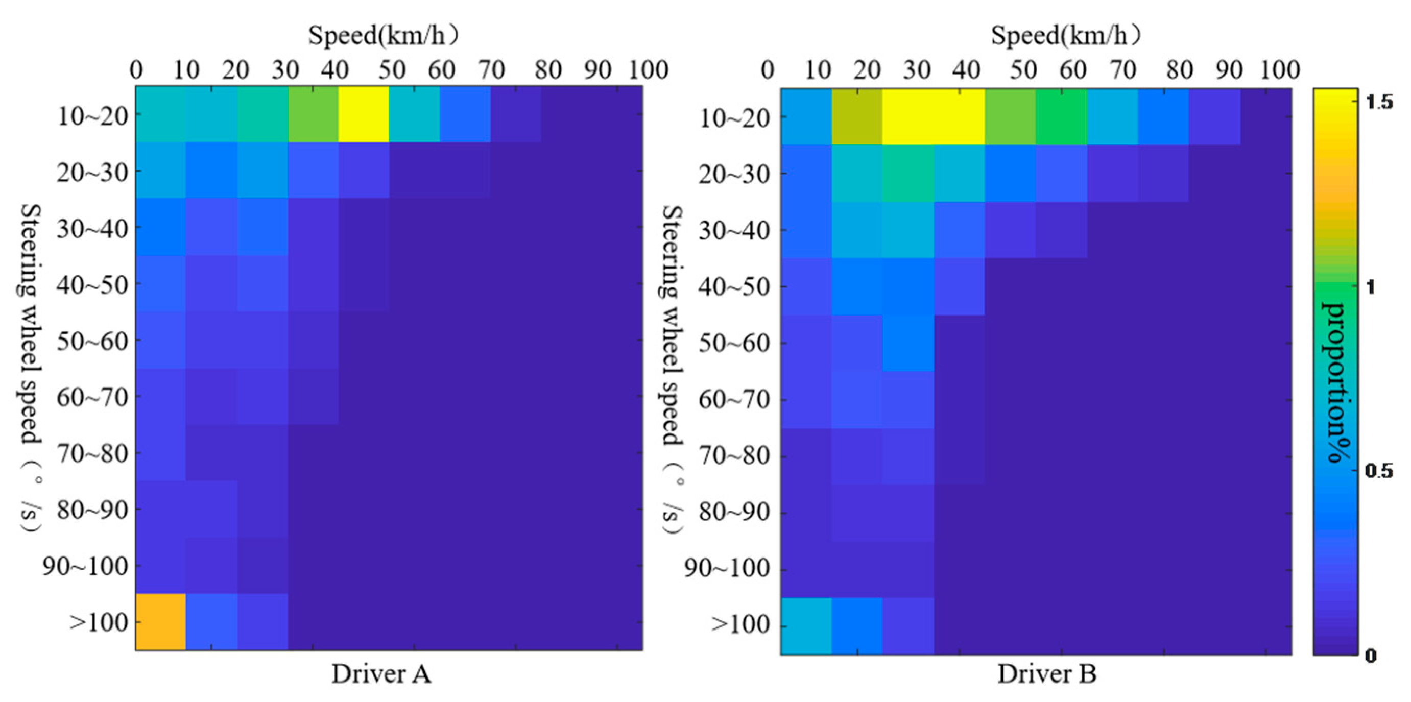
Taking a trip of driver A and a trip of driver B as examples, the joint distribution characteristic parameters of vehicle speed and longitudinal acceleration, braking deceleration, or steering wheel speed are extracted, respectively, as shown in Figure 2, Figure 3 and Figure 4.

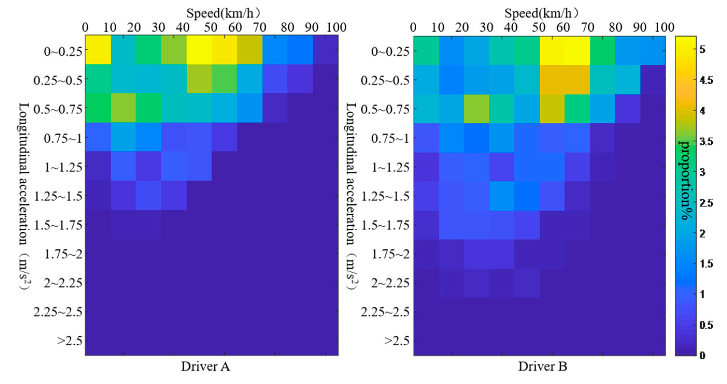
In Figure 2, when the steering wheel speed is higher than 20°/s, the vehicle speed of driver A is concentrated below 30 km/h, whereas the vehicle speed of driver B is concentrated in the range of 10–50 km/h. Figure 2 shows that the turning speed of driver B is higher than driver A. It can be seen from Figure 3 and Figure 4 that the joint distribution between vehicle speed–longitudinal acceleration and vehicle speed–brake deceleration of driver B is relatively scattered, and the vehicle speed, longitudinal acceleration, and braking deceleration are all higher than that of driver A. Figure 3 and Figure 4 show that the driving style of driver B is more intense than driver A.

3.3. Optimization of Driving Style Characteristic Parameters

The driving style characteristic parameters of this paper include a plurality of statistical parameters of NEV big data, the percentage of intervals, and three different joint distribution characteristics, totaling 383 dimensions. In order to minimize the resources required for calculation and maximize the retention of the information contained in the driving behavior characteristic parameters, the characteristic parameters need to be optimized for dimensionality reduction.

In this paper, we used principal component analysis algorithm to orthogonally transform the characteristic parameters of driving behavior. The characteristic parameters that may have a certain correlation with each other can be transformed into a linear and uncorrelated principal component. As shown in Figure 5, the cumulative contribution rate of the first 35 principal components is over 85%. Therefore, the first 35 principal components can be used to represent the driving styles. The dimensionality reduction optimization processing reduces the complexity of the characteristic parameter matrix and can improve the calculation efficiency.

3.4. Automatic Classification of Driving Style

At present, the driving behaviors are usually divided into aggressive, normal, and mild driving behaviors based on the intensity of driving. Based on the characteristic parameters of driving behaviors in this paper, we use the clustering algorithm to realize the automatic classification of driving behavior intelligently and objectively.

The K-means algorithm randomly selects K points from the dataset as cluster center points, calculates the Euclidean distance between the data points of dataset and the cluster center points, and assigns them to the cluster center point with the smallest Euclidean distance. Then, it replaces original cluster center with the mean value of K-cluster, and iterates until the cluster center point remains unchanged or the sum of the squared errors reach local minimum. Among them, the formula for calculating Euclidean distance is

$$d=\sqrt{{\displaystyle \sum _{i=1}^n{(x_i-k_i)}^2}}$$

(1)

where d is the Euclidean distance from the data point to the cluster center point, n is the dimension of the data point, x_i is the characteristic parameter of the data point, and k_i is the characteristic parameter of the cluster center point.

The sum of the squared errors refers to the sum of clustering errors of all data points in the dataset, which can represent the clustering effect to a certain extent. The calculation formula is

$$SSE={\displaystyle \sum _{i=1}^k{\displaystyle \sum _{x\in C_i}{\left|x-k_i\right|}^2}}$$

(2)

where SSE is the sum of squares of errors, C_i represents the i-type of data, k_i is the cluster center point of C_i, and x is any point in the i-type of dataset.

3.5. Driving Style Recognition Model Construction

By K-means clustering algorithm, driving behavior is divided into five categories, and category labels are automatically generated. The classification results and data labels can be used as a training dataset for building a driving style recognition model. In this paper, BP neural network algorithm, which has strong inductive ability, is used to build a driving style model. BP neural network algorithm can obtain hidden data relationships from training data without prior assumptions, and deal with problems with unclear rules or complex internal relationships. The training optimization method of BP neural network is the gradient descent method. The input data of each neuron is

$$net={\displaystyle \sum _{i=1}^n{x}_i{w}_i}$$

(3)

where x_i is the input feature and w_i is the connection weight.

If the Sigmoid function is used as the activation function, the hidden layer neuron output is

$$y^{\prime }=f(net)=\frac{1}{1+e^{-net}}$$

(4)

The training process of BP neural network includes forward propagation of information and back propagation of error. In the forward propagation process, the input of the previous layer is weighted, and becomes the input of the next layer, namely net. In the back propagation process, according to the difference between the actual output y′ and the ideal output y, the weight matrix is adjusted to minimize the error, and finally the error is controlled within a certain required range. The error of the sample data can be described as

$$E_p=\frac{1}{2}{\displaystyle \sum _{j=1}^m{(y_{pj}-O_{pj})}^2}$$

(5)

The total error of the sample data set is $E={\displaystyle \sum E_P}$. The algorithm will iterate until the parameters meet the requirements.

4. Results and Discussions

In this paper, the model was built and solved by Python. The output results are the driving behavior levels of all of the driving behavior fragments.

In theory, the larger the K value of the cluster number, the more accurate the classification. However, the larger K value is not conducive to the classification and analysis of real data. Therefore, it is necessary to first define the optimal cluster number K value. 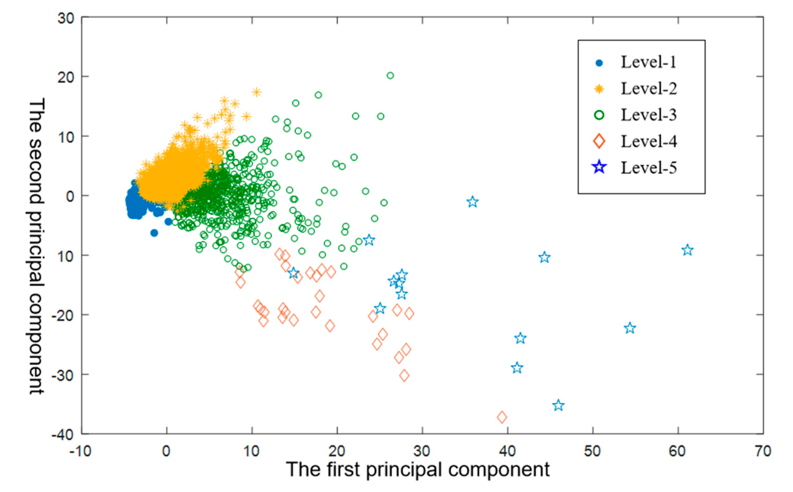In this paper, we test the clustering effect of different clustering numbers K based on the driving behavior feature parameter set after the dimensionality reduction, as shown in Figure 6. When K is less than 5, SSE drops sharply, indicating that, as K increases, the clustering effect is significantly improved. When K is greater than 5, the downward trend of SSE gradually weakens, indicating that the increase in K does not obviously improve the clustering effect. Therefore, we use 5 as the optimal number of clusters, and divide driving style into 5 levels, as shown in Figure 7.

There are 4563 effective driving fragments in the high-frequency big data of this paper. Seventy percent of them are selected randomly as training samples, and the remaining 30% are selected as test samples. In order to speed up the learning process and avoid training non-convergence, the feature vector parameters are standardized and limited to the interval [0, 1].

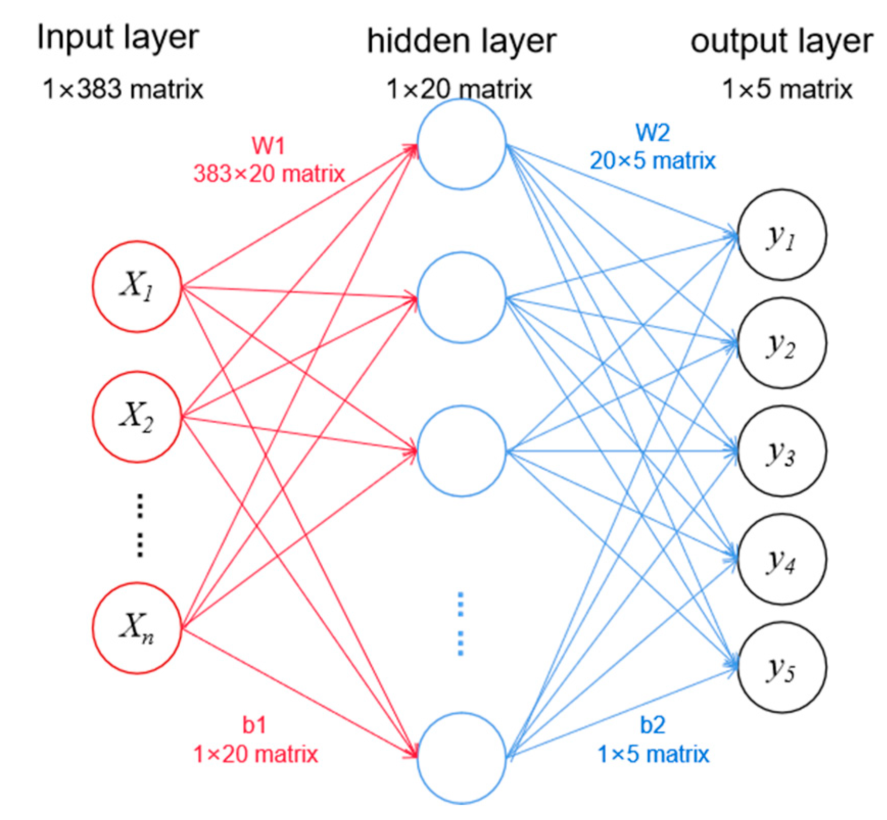
After experimental testing, a three-layer neural network driving style recognition model is established, as shown in Figure 8. In Figure 8, X_i is a input layer node and represents a driving parameter, and y_i is an output layer node and represents the driving style level. The input layer has 383 driving style characteristic parameters, the output layer has 5 driving style levels, and the number of hidden layer nodes is 20. We select the BP algorithm training function tradingdx for network training, define the training parameters, and train the network combined with the number of hidden layer nodes in order to determine the driving style model parameters. The training parameters include a maximum network training times of 10,000, a learning rate of 0.02, and a target error of 1.0 × 10⁻⁸.

We apply the driving behavior recognition model in Figure 8 to the dataset of this paper, and recognize the driving styles of the 4563 effective driving fragments. In the results, 4417 driving styles are the same as in Figure 7, and the recognition accuracy is 96.8%.

This paper uses joint distribution parameters and statistical parameter characteristic parameter sets. The characteristic parameter has 383 dimensions, among which, the joint distribution parameter has 320 dimensions, and the traditional statistical characteristic parameter has only 63 dimensions, as shown in

Table 2. The 63-dimension statistical characteristic parameters.

Speed		Steering Wheel Speed		Longitudinal Acceleration		Braking Deceleration
Maximum		Maximum		Maximum		Maximum
Mean		Mean		Mean		Mean
Mode		Mode		Mode		Mode
Common value		Common value		Common value		Common value
Standard deviation		Standard deviation		Standard deviation		Standard deviation
Ratio of range (km/h)	[0, 10)	Ratio of range (°/s)	[0, 10)	Ratio of range (m/s2)	[0, 0.25)	Ratio of range (m/s2)	[0, 0.25)
	[10, 20)		[10, 20)		[0.25, 0.5)		[0.25, 0.5)
	[20, 30)		[20, 30)		[0.5, 0.75)		[0.5, 0.75)
	[30, 40)		[30, 40)		[0.75, 1)		[0.75, 1)
	[40, 50)		[40, 50)		[1, 1.25)		[1, 1.25)
	[50, 60)		[50, 60)		[1.25, 1.5)		[1.25, 1.5)
	[60, 70)		[60, 70)		[1.5, 1.75)		[1.5, 1.75)
	[70, 80)		[70, 80)		[1.75, 2)		[1.75, 2)
	[80, 90)		[80, 90)		[2, 2.25)		[2, 2.25)
	[90, 100)		[90, 100)		[2.25, 2.5)		[2.25, 2.5)
	-		[100, ∞)		[2.5, ∞)		[2.5, ∞)

. Compared with the traditional driving behavior recognition method that only uses statistical feature parameters, this paper adds 320-dimension joint distribution feature parameters, which can describe the correlation between the vehicle speed and the steering wheel speed, acceleration, and deceleration during the driving stage. For example, in Figure 2, when the steering wheel speed is in the range of 10–20°/s, the speed distributions of driver A and driver B are different, which expresses the difference in the driving style of the two drivers. Only statistical parameters extracted for the vehicle speed or steering wheel angle cannot express this information.

In order to discuss the influence of the feature parameter set on the driving style recognition result, we built a driving style recognition model using 63-dimension statistical feature parameters using the same method in Figure 8. The number of input layer nodes is the same as the dimension of feature parameters, and the number of output layer nodes is the same as the number of driving style levels. Due to the reduction of input feature parameters, the number of nodes in the input layer of this model is reduced to 63. However, since the driving behavior is still divided into five levels according to Figure 7, the number of nodes in the output layer remains unchanged. The number of nodes in the input layer is reduced, and the complexity of the model solution is reduced, so we redefine the number of nodes in the hidden layer to 10. Compared with the model in Figure 8, the complexity of the new model is reduced, and the computing resources occupied are reduced. The parameters of the two driving behavior recognition models are shown in Table 2.

Using the statistical parameters model and the 63-dimension statistical parameters of 4563 driving behavior fragments for driving style recognition, 4248 fragments can be correctly recognized, as shown in

Table 3. Comparison of models and results.

Comparison Item		Joint Distribution Parameters Sets	Statistical Parameters
Dimensions		383	63
Models	Input layer	383	63
	Hidden layer	20	10
	Output layer	5	5
Results	Number of accurately identified fragments	4417	4248
	Recognition accuracy	96.8%	93.1%

. Compared with the joint analysis parameter sets model, the number of correct recognition fragments is reduced by 169. Most of the 169 driving behaviors with recognition errors are level 1, level 2, and level 3. In our opinion, the reason for the recognition error is that their statistical parameters are close to each other, and the subtle differences between driving behaviors in level 1 to level 3 cannot be distinguished.

The focus of this paper is to use new joint distribution feature parameters to represent driving behavior, instead of conventional statistical parameters, and to build a driving style recognition model based on these new parameters. We use the BP neural network algorithm because the BP algorithm has a strong generalization ability. Furthermore, the new joint distribution feature parameters can be applied to other modeling algorithms, such as SVM, random forest, Tri-CatBoost, ELM, etc.

It should be noted that we need to extract the joint distribution characteristic parameters from NEV high-frequency big data, so the method in this paper is not suitable for the low-frequency real-time big data currently being collected by the new energy vehicle industry in China. In addition, NEV high-frequency big data requires much higher storage equipment and computing resources than low-frequency data.

5. Conclusions

Driving behavior has an impact on safety, energy consumption, and battery life. A deep understanding of driving style will have important guiding significance for the innovative development of new energy vehicles. This paper studies a NEV driving style recognition model relying on high-frequency big data, and extracts the joint distribution characteristic parameters of different data types, which can more fully reflect the temporal and spatial characteristics of driving behavior. The model has been tested with real-world driving segment data, and the accuracy can reach 96.8%.

Next, we will expand the sample size of driving fragments and analyze the correlation between the driving style and energy consumption of NEV in order to improve the quality of research results and clarify the impact of driving style on energy consumption.