The Energy Efficiency of Heterogeneous Cellular Networks Based on the Poisson Hole Process

Abstract

In order to decrease energy consumption caused by the dense deployment of pico base stations (PBSs) in heterogeneous cellular networks (HetNets), this paper first analyzes the energy efficiency (EE) of two-tier HetNets and then proposes a method to maximize the network EE by adjusting the PBS transmit power. The two-tier HetNets are modeled by the Poisson point process (PPP) and the Poisson hole process (PHP), and then the coverage probability of the macro base station (MBS) and the PBS in the two-tier HetNets is derived based on the mean interference to signal ratio (MISR). According to the user association probability, the coverage probability of the PPP-PHP HetNets is obtained. Then, the tractable expression of the average achievable rate is deduced on the basis of the relationship between the coverage probability and the average achievable rate. Finally, the expression of EE is derived and the EE optimization algorithm is proposed based on the PBS transmit power. The simulation results show that the PPP-PHP network is superior to the PPP-PPP network in terms of coverage probability and EE, and the network EE can be effectively improved by setting an appropriate PBS transmit power.

1. Introduction

The intelligent application driven by the fourth industrial revolution forces the user demand to grow exponentially. The rapid growth of mobile data services has brought great challenges to traditional cellular networks. The LTE [1] and WiMax [2] standard groups propose the introduction of some low-power nodes to expand the system capacity [3,4], offload macro base station (MBS) traffic [5,6], enhance indoor coverage, and improve the service quality of the cell edge users [7]. The network architecture composed of macro stations and low-power nodes is called the heterogeneous cellular network (HetNet). The HetNet has been identified as the network architecture of the fifth-generation cellular mobile communication [8,9], which integrates a variety of different types of base stations, including the MBS, the pico base station (PBS), the home base station (Femto), and the wireless relay node (Relay) with backhaul link [10,11].

The deployment of small cells brings many benefits but also brings disadvantages, such as increased energy consumption and network management difficulties. Although the power consumption of small-cell base stations is relatively low, ultra-dense deployment will increase the energy consumption of the system [12,13]. In 2025, due to the 5G high-density network technology, the energy consumption and carbon dioxide emissions of small communities will increase significantly, and the increase in carbon dioxide emissions will have adverse effects on the environment and human health. In network and communication technology, reducing energy consumption is a key challenge at present.

1.1. Related Works

As cellular networks tend to be more and more heterogeneous and the spatial distribution of sites is more and more random, research on heterogeneous cellular networks based on stochastic geometry has become more necessary. The Poisson point process (PPP) has been widely used in the modeling and analysis of cellular networks due to its mathematical tractability. However, the PPP assumes that the BSs are independent, which deviates from the actual network deployment. Therefore, the analysis results are more ideal. To solve the modeling of network deployment, some studies propose using the non-Poisson point process with spatial exclusion or aggregation to model the different spatial correlations of realistic HetNets. The Ginibre point process (GPP) [14,15] and the Matérn hard-core point process (MHCPP) [16] are used to fit the exclusivity between the BSs of the same tier. The Matern cluster process (MCP) [17,18] and the Poisson cluster process (PCP) [19,20] are used to fit the clustering characteristics of small base stations. The Poisson hole process (PHP) is used to fit the repulsion between MBSs and small base stations (SBSs) [21,22]. It is very difficult to accurately calculate the signal-to-interference ratio (SIR) distribution of cellular networks through the non-Poisson point process. In the cellular network modeled by the GPP, the calculation of the SIR is relatively simple, but the combination of the infinite sum and the integral also appears in the precise expression of its complementary cumulative distribution function, and the network analysis based on other non-Poisson point processes is more complex, which makes its performance analysis more challenging. To solve this problem, references [23,24,25] proposed that the SIR based on the non-Poisson point process network can be accurately approximated by the SIR distribution of the PPP network; this method is also called “PPP-based approximate SIR analysis” (ASPPP), which provides an effective analysis method for analyzing the performance of the actual network.

For future mobile communication systems, research on network structures and transmission mechanisms to save energy and improve energy efficiency (EE) is a widespread concern in academic and industrial circles [26,27,28,29]. The following section summarizes the current status of improving network EE from the aspects of BS deployment, BS sleep, and power allocation.

The authors of [30] indicated that the transmit power of the MBS, the distance between the BSs, and the number of BSs have an impact on the EE of the system. The proper selection of these parameters can ensure significant energy savings. In addition, adding PBSs in HetNets can help improve network EE. Moreover, [31] analyzed the EE of two-tier heterogeneous wireless networks from the perspective of PBS deployment, and studied whether deploying PBSs can increase system capacity and save energy from the aspects of area spectrum efficiency and area power consumption. The authors of [32] studied the SE and EE of a two-tier heterogeneous network, in which the MBS and the PBS are modeled by two independent PPPs. The results show that deploying PBSs in macro cells is an effective method to improve the SE of the network. When the density of PBSs does not exceed the optimum, the EE of the whole network can be effectively improved. The authors of [33] deduced the local delay and EE of heterogeneous networks when BSs are modeled by the PPP and the PCP. Due to the existence of intra-cluster interference, the local delay and EE of BS deployment modeled by the PCP are greater than those modeled by the PPP. In [34], the distribution of small cells is modeled by the MCP. A general formula for the lower bound of the average reachability rate is derived and the optimal number of cell clusters to maximize EE is studied.

BS sleep is also an important technology used to reduce energy consumption in HetNets. The authors of [35,36,37] improved the energy efficiency of the network through BS on/off switching and transmission power scaling. The authors of [38] proposed a SBS sleep scheme, which determines whether the SBS is in sleep state according to the system throughput. The simulation results show that, compared with the traditional scheme, this scheme can effectively reduce the total power consumption of the network and improve the energy efficiency of the system. Li Yun et al. studied the joint sleep strategy based on the MBS density and the SBS density [39]. The authors of [40] designed an optimization model to schedule the four states of the base station (activation, waiting, deep sleep, and shutdown) by maintaining the minimum quality of service required by users, so as to minimize power consumption. The simulation results show that the proposed model has better performance than the existing methods. By reducing the percentage of active small cells, the power consumption is reduced to about 10%.

Optimizing the transmit power of base stations is also a feasible way to improve the EE of HetNets. The authors of [41] developed a joint interference and power management mechanism to reduce signal interference and save energy of user equipment and improve LTE-A performance. The authors of [42] used game theory to solve the optimal unit selection and uplink power control problems of open-access two-tier femtocell networks. The authors of [43] studied the EE of two-tier HetNets, in which the BS was modeled as the PPP, the impact of the BS transmit power on the EE was analyzed, and an algorithm used to find the best PBS transmit power to maximize EE was proposed. On this basis, the authors of [44] proposed to maximize the network EE through the joint optimization of the PBS density and transmit power. The authors of [45] studied the EE of two-tier HetNets based on the spatial repulsion of BSs in the same tier, in which the deployment of MBSs is modeled by the β-Ginibre point process, and proposed an EE optimization algorithm to determine the optimum transmit power of PBS to improve the EE of HetNets.

In this paper, the performance of HetNets is studied from the inter-tier correlation. Different from the modeling deployment in [43,44,45], the MBS deployment is modeled by PPP, and the PBSs are deployed outside the exclusion zone of the given radius of the MBS. In this case, the deployment of the PBS follows the PHP distribution. Introducing repulsion can reduce the interference to the MBS when the PBS is transmitted. This paper studies the energy efficiency of two-tier heterogeneous cellular networks and optimizes the EE by adjusting the PBS transmit power. First, the coverage probability and the average achievable rate of two-tier PPP-PHP HetNets are derived based on the ASPPP method. Secondly, according to the definition of the network energy efficiency and the energy consumption model of the base station, the expression of the network energy efficiency in relation to the base station transmit power is derived. Finally, it is optimized according to the proposed energy efficiency optimization algorithm.

1.2. Paper Organization

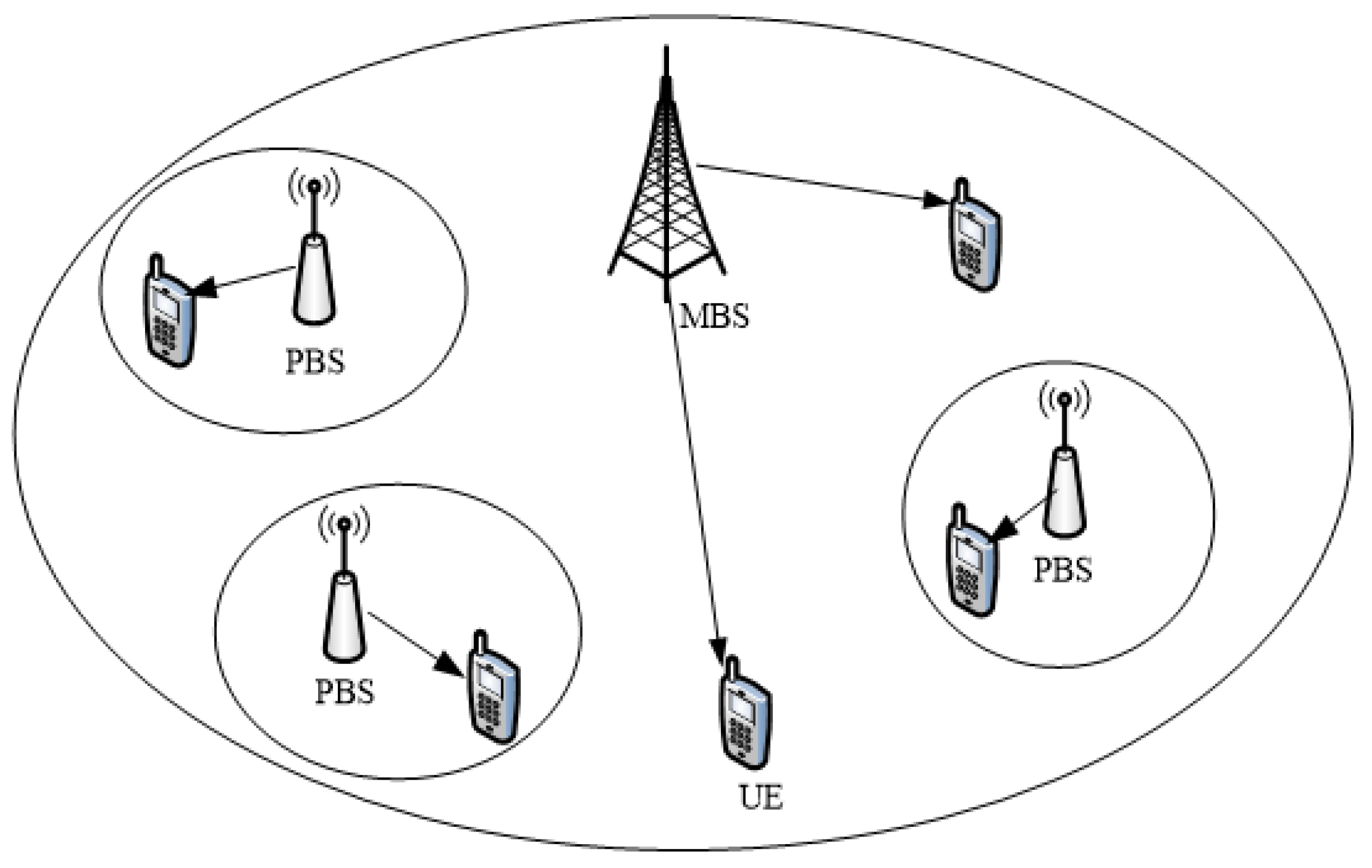
The rest of this paper is arranged as follows: Section 2 introduces the system model. In Section 3, the expressions of coverage probability and average achievable rate of HetNets are derived and the expression of network energy efficiency is derived according to the definition. In Section 4, a quadratic interpolation algorithm is proposed to optimize energy efficiency. The simulation results are discussed in Section 5 and the conclusions are given in Section 6.

2. System Model

The two-tier HetNets, composed of MBSs and PBSs, are considered, as shown in Figure 1.

The deployment of the MBS follows the PPP ${\mathsf{\Phi }}_m$ distribution, and its density is ${\lambda }_m$, and the deployment of the PBS follows the PHP ${\mathsf{\Phi }}_p$ distribution, and its density is ${\lambda }_p$. The generation process of the PHP can be expressed as follows: suppose ${\tilde{\mathsf{\Phi }}}_p$ is an independent uniform PPP with density ${\tilde{\lambda }}_p$, let ${\mathsf{\Xi }}_r=\cup \{x\in {\mathsf{\Phi }}_m:b(x,r)\}$, where ${\mathsf{\Xi }}_r$ is the union of all disks in ${\mathsf{\Phi }}_m$, with x as the center and R as the radius. The Poisson hole process ${\mathsf{\Phi }}_p$ is expressed as ${\mathsf{\Phi }}_p=\{x\in {\tilde{\mathsf{\Phi }}}_p:x\notin {\mathsf{\Xi }}_r\}={\tilde{\mathsf{\Phi }}}_p\backslash {\mathsf{\Xi }}_r$, i.e., the point process made up of the remaining points after removing all points in the ${\mathsf{\Xi }}_r$ area in ${\tilde{\mathsf{\Phi }}}_p$, and its density is ${\lambda }_p={\tilde{\lambda }}_p\exp (-{\lambda }_m\pi r^2)$. The base station distribution diagram of the HetNets is shown in Figure 2, where ${\lambda }_m=0.001$ m⁻², ${\tilde{\lambda }}_p=0.01$ m⁻², r = 5 m, and the network area is 10,000 m².

The transmit powers of the MBS and the PBS are denoted by ${\mu }_m$ and ${\mu }_p$, respectively. The network model is stationary because the entire Poisson point process is moved and the position of the typical user is at the center origin; according to the Palm distribution and the Slivnyak theorem in stochastic geometry, the conditional distribution at this time still follows the Poisson point process of the same density and all users have the same statistical characteristics, so only the typical users at the origin are considered. Considering the open-access mode, the average maximum received power is used as the criterion for the associated base station and the received power of the user-associated service base station can be expressed as ${\mu }_k{h}_{k0}|x_0{|}^{-\alpha }$, where the path loss factor $\alpha >2$,$k\in \{m,p\}$, x₀ is the location of the service base station in ${\mathsf{\Phi }}_k$, which also represents the distance between the typical user and the service BS, and h_k0 is the channel gain. This paper assumes that the fast fading is Rayleigh fading, i.e., h_k0 ~ exp (1), and ${\mu }_k$ indicates the transmit power of the k-th tier base station associated with a typical user. In light of general frequency reuse, the signals received by a typical user from base stations other than the service base station are regarded as interfering signals. In heterogeneous networks with limited interference, the noise power can be ignored. Then, the user SIR associated with the service base station located at $x_0\in {\mathsf{\Phi }}_k$ is:

$$SI{R}_k=\frac{{\mu }_k{h}_{k0}|x_0{|}^{-\alpha }}{{\displaystyle \sum _{x_i\in {\mathsf{\Phi }}_m\backslash \left\{x_0\right\}}{\mu }_m{h}_{mi}|x_i{|}^{-\alpha }+{\displaystyle \sum _{x_i\in {\mathsf{\Phi }}_p\backslash \left\{x_0\right\}}{\mu }_p{h}_{pi}|x_i{|}^{-\alpha }}}}$$

(1)

We list the main notations used in the paper in

Table 1. Summary of notations.

Notation	Definition
${\lambda }_m$$,{\lambda }_p$	Deployment density of the MBS/PBS
${\mathsf{\Phi }}_m$$,{\mathsf{\Phi }}_p$	Point process for modeling MBS/PBS location
$\theta$	Given threshold of the BS
${\mu }_m$$,{\mu }_p$	MBS/PBS transmit power
$A_m$$,A_p$	The probability that a typical user is associated with the MBS/PBS
r	Repulsion radius
PCm, PCp	The coverage probability of the MBS/PBS
$f_m(r_0)$$,f_p(r_0)$	The distance distribution between the service MBS/PBS and the typical user
${\tau }_m$$,{\tau }_p$	The average achievable rate of the typical user associated with the MBS/PBS
$N_m$$,N_p$	The number of users served by the MBS/PBS
Pm0, Pp0	MBS/ PBS static power consumption
${\eta }_{EE}$	Energy efficiency

.

3. Energy Efficiency Analysis

3.1. Coverage Probability

In the downlink HetNets with limited interference, the coverage probability is defined as the probability that the SIR received by the user is larger than the threshold value. Because users are associated with a certain tier at most, the coverage probability can be taken as the sum of the probabilities of several mutually exclusive events.

In the network model of this paper, the coverage probability can be given by:

$$P_C=P_{Cm}{A}_m+P_{Cp}{A}_p=P_{C\_m}+P_{C\_p}$$

(2)

where $A_m$ and $A_p$ are the probabilities that a typical user is associated with the MBS and the PBS, respectively, and P_Cm and P_Cp are the coverage probabilities of the MBS and the PBS, respectively. P_Cm is denoted as the probability that the SIR_m provided by the service MBS for the typical user is greater than the threshold value ${\theta }_m$, i.e., $P_{Cm}=P(SI{R}_m>{\theta }_m)$. P_Cp is denoted as the probability that the SIR_p provided by the service PBS for the typical user is greater than the threshold value ${\theta }_p$, i.e., $P_{Cp}=P(SI{R}_p>{\theta }_p)$. In this paper, it is assumed that the given thresholds of the MBS and the PBS are the same, which is denoted as $\theta$.

The SIR_m received by a typical user from the MBS is expressed as:

$$\begin{array}{l}SI{R}_m=\frac{{\mu }_m{h}_{m0}|x_0{|}^{-\alpha }}{{\displaystyle \sum _{x_i\in {\mathsf{\Phi }}_m\backslash \left\{x_0\right\}}{\mu }_m{h}_{mi}|x_i{|}^{-\alpha }+{\displaystyle \sum _{x_i\in {\mathsf{\Phi }}_p\backslash \left\{x_0\right\}}{\mu }_p{h}_{pi}|x_i{|}^{-\alpha }}}}\\ =\frac{h_{m0}}{{\displaystyle \sum _{x_i\in {\mathsf{\Phi }}_m\backslash \left\{x_0\right\}}{h}_{mi}|x_0{|}^{\alpha }|x_i{|}^{-\alpha }+{\displaystyle \sum _{x_i\in {\mathsf{\Phi }}_p\backslash \left\{x_0\right\}}\frac{{\mu }_p}{{\mu }_m}{h}_{pi}|x_0{|}^{\alpha }|x_i{|}^{-\alpha }}}}=\frac{h_{m0}}{I_1}\end{array}$$

(3)

The SIR_p received by a typical user from the PBS is expressed as:

$$\begin{array}{l}SI{R}_p=\frac{{\mu }_p{h}_{p0}|x_0{|}^{-\alpha }}{{\displaystyle \sum _{x_i\in {\mathsf{\Phi }}_m\backslash \left\{x_0\right\}}{\mu }_m{h}_{mi}|x_i{|}^{-\alpha }+{\displaystyle \sum _{x_i\in {\mathsf{\Phi }}_p\backslash \left\{x_0\right\}}{\mu }_p{h}_{pi}|x_i{|}^{-\alpha }}}}\\ =\frac{h_{p0}}{{\displaystyle \sum _{x_i\in {\mathsf{\Phi }}_m\backslash \left\{x_0\right\}}\frac{{\mu }_m}{{\mu }_p}{h}_{mi}|x_0{|}^{\alpha }|x_i{|}^{-\alpha }+{\displaystyle \sum _{x_i\in {\mathsf{\Phi }}_p\backslash \left\{x_0\right\}}{h}_{pi}|x_0{|}^{\alpha }|x_i{|}^{-\alpha }}}}=\frac{h_{p0}}{I_2}\end{array}$$

(4)

Based on the SIR threshold model, the coverage probability is equivalent to the complementary cumulative distribution function (CCDF) of the SIR. It has been proven that taking the PPP as a reference model and adopting the SIR threshold scaling method can provide a good approximation to the SIR distribution of the general point process model; in other words, scaling the threshold value $\theta$ of the SIR distribution of the Poisson model network to $\theta /G$ can obtain the SIR distribution of the non-Poisson network. G is called the gain factor, which is defined as the ratio of the MISR of a typical user under the PPP model to the MISR of a typical user under the target model, and its mathematical expression can be written as $G=\frac{MIS{R}_{PPP}}{MISR}$. The MISR of a typical user is defined as:

$$MISR=\mathrm{E}\left\{\frac{I}{{\mathrm{E}}_h(S)}\right\}=\mathrm{E}\left\{\frac{{\displaystyle \sum _{x_i\in {\mathsf{\Phi }}_m\backslash \left\{x_0\right\}}{\mu }_m{h}_{mi}|x_i{|}^{-\alpha }+{\displaystyle \sum _{x_i\in {\mathsf{\Phi }}_p\backslash \left\{x_0\right\}}{\mu }_p{h}_{pi}|x_i{|}^{-\alpha }}}}{{\mu }_k{h}_{k0}|x_0{|}^{-\alpha }}\right\}$$

(5)

where $E_h(s)$ is the average received signal power of a typical user and I is the sum of all interference powers.

Based on this method, this section deduces the coverage probability of the PPP-PHP HetNets. The authors of [46] show that the calculation result of the MISR in the PPP network is $MIS{R}_{PPP}=2/(\alpha -2)$. Assuming that the density of the MBS and the PBS is constant, and the relationship between $MIS{R}_{PHP}$ and the path loss factor α is obtained by simulation and data fitting, $MIS{R}_{PHP}=14.31\times {\alpha }^{-1.99}$ [47]. The gain factor G_p of the HetNets modeled by the PHP can be written as:

$$G_p=\frac{MIS{R}_{PPP}}{MIS{R}_{PHP}}=\frac{2/(\alpha -2)}{1.43\times {\alpha }^{-1.99}}$$

(6)

Next, we use the method based on the MISR to derive the coverage probability of the MBS and the PBS in two-tier HetNets, and then obtain the total coverage probability of the HetNets according to the user association probability.

Theorem 1. 

The coverage probability of the typical user serviced by the MBS in two-tier HetNets is expressed as:

$$P_{Cm}(\theta )=\frac{{\lambda }_m+{\lambda }_p{(\frac{{\mu }_p}{{\mu }_m})}^{2/\alpha }}{{\lambda }_{m}T(\alpha ,\theta )+{\lambda }_p{(\frac{{\mu }_p}{{\mu }_m})}^{2/\alpha }T(\alpha ,\theta )}$$

(7)

Proof. 

P_Cm is denoted as the probability that the SIR_m provided by the service MBS for the typical user is greater than the threshold value ${\theta }_m$, which can be expressed as:

$$\begin{array}{l}{P}_{Cm}(\theta )=P(SI{R}_m>\theta )={\displaystyle \underset{r_0>0}{\int }P(h_{m0}>\theta I_1|r_0)f_m(r_0)d{r}_0}\\ ={\displaystyle \underset{r_0>0}{\int }{E}_{I_1}[e^{-\theta I_1}}]f_m(r_0)d{r}_0={\displaystyle \underset{r_0>0}{\int }{L}_{I_1}(\theta )f_m(r_0)}d{r}_0 \end{array}$$

(8)

where $f_m(r_0)$ denotes the distance distribution between the service MBS and the typical user.

$$f_m(r_0)=2\pi r_0({\lambda }_m+{\lambda }_p{({\mu }_p/{\mu }_m)}^{2/\alpha })\exp (-{\lambda }_m\pi r_0^2-{\lambda }_p\pi {({\mu }_p/{\mu }_m)}^{2/\alpha }{r}_0^2)$$

(9)

$$\begin{array}{l}{L}_{I_1}(\theta )=E_{I_1}[e^{-\theta \cdot I_1}]=E_{I_1}[e^{-\theta ({\displaystyle \sum _{x_i\in {\mathsf{\Phi }}_m\backslash \left\{x_0\right\}}{h}_{mi}{r}_0^{\alpha }|x_i{|}^{-\alpha }+{\displaystyle \sum _{x_i\in {\mathsf{\Phi }}_p\backslash \left\{x_0\right\}}\frac{{\mu }_p}{{\mu }_m}{h}_{pi}{r}_0^{\alpha }|x_i{|}^{-\alpha }}})}]\\ \stackrel{(a)}{\ge }{E}_{{\mathsf{\Phi }}_m,h_{mi}}[{\displaystyle \prod _{x_i\in {\mathsf{\Phi }}_m\backslash \left\{x_0\right\}}\exp (}-\theta \cdot h_{mi}{r}_0^{\alpha }|x_i{|}^{-\alpha })]\cdot E_{{\mathsf{\Phi }}_p,h_{pi}}[{\displaystyle \prod _{x_i\in {\left\{{\mathsf{\Phi }}_p\backslash \left\{x_0\right\}\right\}}^{PPP}}\exp (}-\theta \frac{{\mu }_p}{{\mu }_m}{h}_{pi}{r}_0^{\alpha }|x_i{|}^{-\alpha })]\\ \stackrel{(b)}{=}\exp (-2\pi {\lambda }_m{\displaystyle {\int }_{r_0}^{\infty }(1-}{L}_{h_{mi}}(\theta \cdot r_0^{\alpha }|x{|}^{-\alpha }))xdx)\cdot \exp (-2\pi {\lambda }_p{\displaystyle {\int }_{r_0}^{\infty }(1-}{L}_{h_{pi}}(\theta \frac{{\mu }_p}{{\mu }_m}{r}_0^{\alpha }|y{|}^{-\alpha }))ydy)\\ \stackrel{(c)}{=}\exp (-2\pi {\lambda }_m{\displaystyle {\int }_{r_0}^{\infty }(1-}\frac{1}{1+\theta \cdot r_0^{\alpha }|x{|}^{-\alpha }})xdx)\cdot \exp (-2\pi {\lambda }_p{\displaystyle {\int }_{r_0}^{\infty }(1-}\frac{1}{1+\theta \frac{{\mu }_p}{{\mu }_m}{r}_0^{\alpha }|y{|}^{-\alpha }})ydy)\\ \stackrel{(d)}{=}\exp (-\pi {\lambda }_m{r}_0^2(T(\alpha ,\theta )-1))\cdot \exp (-\pi {\lambda }_p{r}_0^2{(\frac{{\mu }_p}{{\mu }_m})}^{2/\alpha }(T(\alpha ,\theta )-1)) \end{array}$$

(10)

where (a) the interference generated by ${\mathsf{\Phi }}_P^{PPP}$ with the same density is used to replace the interference generated by ${\mathsf{\Phi }}_P$, and the lower bound of coverage probability is obtained, (b) according to the probability generating function (PGF) [48] of the PPP network, (c) the channel gain obeys Rayleigh fading, i.e., $h_{mi}~\exp (1)$ and $h_{pi}~\exp ( 1)$, and (d) let $T(\alpha ,\theta )=1+{\theta }^{2/\alpha }{\displaystyle {\int }_{{\theta }^{-2/\alpha }}^{\infty }(1-{(1+u^{-\alpha /2})}^{-1})du}$.

By substituting Formulas (9) and (10) into Formula (8), the coverage probability $P_{Cm}$ of the MBS in the two-tier HetNets can be obtained. □

Theorem 2. 

The coverage probability of the typical user serviced by the PBS in two-tier HetNets is given by:

$$P_{Cp}(\theta )=\frac{{\lambda }_p+{\lambda }_m{(\frac{{\mu }_m}{{\mu }_p})}^{2/\alpha }}{{\lambda }_m{(\frac{{\mu }_m}{{\mu }_p})}^{2/\alpha }T(\alpha ,\theta )+{\lambda }_{p}T(\alpha ,\frac{\theta }{G_p})}$$

(11)

Proof. 

P_Cp is denoted as the probability that the SIR_p provided by the service PBS for the typical user is greater than the threshold value ${\theta }_p$, which can be expressed as:

$$\begin{array}{l}{P}_{Cp}(\theta )=P(SI{R}_p>\theta )={\displaystyle \underset{r_0>0}{\int }P(h_{p0}>\theta I_2|r_0)f_p(r_0)d{r}_0}\\ ={\displaystyle \underset{r_0>0}{\int }{E}_{I_2}[e^{-\theta I_2}}]f_p(r_0)d{r}_0={\displaystyle \underset{r_0>0}{\int }{L}_{I_2}(\theta )f_p(r_0)}d{r}_0 \end{array}$$

(12)

where $f_p(r_0)$ denotes the distance distribution between the service PBS and the typical user.

$$f_p(r_0)=2\pi r_0({\lambda }_p+{\lambda }_m{({\mu }_m/{\mu }_p)}^{2/\alpha })\exp (-{\lambda }_p\pi r_0^2-{\lambda }_m\pi {({\mu }_m/{\mu }_p)}^{2/\alpha }{r}_0^2)$$

(13)

$$\begin{array}{l}{L}_{I_2}(\theta )=E_{I_2}[e^{-\theta ({\displaystyle \sum _{x_i\in {\mathsf{\Phi }}_m\backslash \left\{x_0\right\}}\frac{{\mu }_m}{{\mu }_p}{h}_{mi}|x_0{|}^{\alpha }|x_i{|}^{-\alpha }+{\displaystyle \sum _{x_i\in {\mathsf{\Phi }}_p\backslash \left\{x_0\right\}}{h}_{pi}|x_0{|}^{\alpha }|x_i{|}^{-\alpha }}})}]\\ \stackrel{(a)}{~}{E}_{{\mathsf{\Phi }}_m,h_{mi}}[{\displaystyle \prod _{x_i\in {\mathsf{\Phi }}_m\backslash \left\{x_0\right\}}\exp (}-\theta h_{mi}{r}_0^{\alpha }|x_i{|}^{-\alpha })]\cdot E_{{\mathsf{\Phi }}_p,h_{pi}}[{\displaystyle \prod _{x_i\in {\left\{{\mathsf{\Phi }}_p\backslash \left\{x_0\right\}\right\}}^{PPP}}\exp (}-\frac{\theta }{G_p}{h}_{pi}{r}_0^{\alpha }|x_i{|}^{-\alpha })]\\ \stackrel{(b)}{=}\exp (-2\pi {\lambda }_m{\displaystyle {\int }_{r_0}^{\infty }(1-}{L}_{h_{mi}}(\theta \cdot \frac{{\mu }_m}{{\mu }_p}{r}_0^{\alpha }|x{|}^{-\alpha }))xdx)\cdot \exp (-2\pi {\lambda }_p{\displaystyle {\int }_{r_0}^{\infty }(1-}{L}_{h_{pi}}(\frac{\theta }{G_p}{r}_0^{\alpha }|y{|}^{-\alpha }))ydy)\\ \stackrel{(c)}{=}\exp (-\pi {\lambda }_m{r}_0^2{(\frac{{\mu }_m}{{\mu }_p})}^{2/\alpha }(T(\alpha ,\theta )-1))\cdot \exp (-\pi {\lambda }_p{r}_0^2(T(\alpha ,\frac{\theta }{G_p})-1)) \end{array}$$

(14)

where (a) the MISR-based approximation method is used, i.e., to replace $\theta$ with $\frac{\theta }{G_p}$, and the distribution of user-received SIR in the network modeled by PHP can be accurately approximated by the PPP network, (b) according to the PGF of the PPP network, (c) the channel gain follows Rayleigh fading, i.e., $h_{mi}~\exp (1)$, and $h_{pi}~\exp ( 1)$, and $T(\alpha ,\theta )=1+{\theta }^{2/\alpha }{\displaystyle {\int }_{{\theta }^{-2/\alpha }}^{\infty }(1-{(1+u^{-\alpha /2})}^{-1})du}$, which can be derived.

By substituting Formulas (13) and (14) into Formula (12), we obtained the coverage probability of the PBS in two-tier HetNets.

In [49], it is assumed that the user adopts open-access mode, i.e., whereby the user is allowed to associate with the BS of any tier. The probability that a typical user is associated with a particular tier depends on the density of the BS and the transmit power of the BS. The probability of a typical user associated with an MBS is expressed as:

$$A_m=\frac{{\lambda }_m{\mu }_m{}^{2/\alpha }}{{\lambda }_m{\mu }_m{}^{2/\alpha }+{\lambda }_p{\mu }_p{}^{2/\alpha }}$$

(15)

The probability of a typical user associated with a PBS is expressed as:

$$A_p=\frac{{\lambda }_p{\mu }_p{}^{2/\alpha }}{{\lambda }_m{\mu }_m{}^{2/\alpha }+{\lambda }_p{\mu }_p{}^{2/\alpha }}$$

(16)

By substituting Formulas (7), (11), (15), and (16) into Formula (2), we can obtain the coverage probability of two-tier PPP-PHP HetNets:

$$\begin{array}{l}{P}_C=P_{Cm}{A}_m+P_{Cp}{A}_p=P_{C\_m}+P_{C\_p}\\ =\frac{1}{T(\alpha ,\theta )+\frac{{\lambda }_p}{{\lambda }_m}{(\frac{{\mu }_p}{{\mu }_m})}^{2/\alpha }T(\alpha ,\theta )}+\frac{1}{\frac{{\lambda }_m}{{\lambda }_p}{(\frac{{\mu }_m}{{\mu }_p})}^{2/\alpha }T(\alpha ,\theta )+T(\alpha ,\frac{\theta }{G_p})}\end{array}$$

(17)

□

3.2. Average Achievable Rate

Suppose ${\tau }_m$ and ${\tau }_p$ are used to denote the average achievable rate of the typical user associated with the MBS and the PBS and expressed as follows, respectively:

$${\tau }_m=\mathrm{E}[\log (1+SI{R}_m)]$$

(18)

$${\tau }_p=\mathrm{E}[\log (1+SI{R}_p)]$$

(19)

Theorem 3. 

The average achievable rate of the typical user associated with the MBS is expressed as:

$${\tau }_m={\displaystyle {\int }_0^{\infty }\frac{1}{z}}(1-e^{-z})\frac{1}{H\left(z\right)}dz$$

(20)

Proof. 

The deployment of the MBS is modeled by the PPP, and the average achievable rate of the typical user associated with the MBS is written as:

$$\begin{array}{l}{\tau }_{{}_m}^{PPP}=\mathrm{E}(\log (1+SI{R}_m)]\\ ={\displaystyle {\int }_0^{\infty }{f}_m}(r_0)E[\log (1+\frac{{\mu }_m{h}_{m0}{r}_0^{-\alpha }}{{\displaystyle \sum _{x_i\in {\mathsf{\Phi }}_m\backslash \left\{x_0\right\}}{\mu }_m{h}_{mi}{x}_i^{-\alpha }+{\displaystyle \sum _{x_i\in {\mathsf{\Phi }}_p\backslash \left\{x_0\right\}}{\mu }_p{h}_{pi}{x}_i^{-\alpha }}}})]d{r}_0\end{array}$$

(21)

where:

$$\begin{array}{l}E[\log (1+\frac{{\mu }_m{h}_{m0}{r}_0^{-\alpha }}{{\displaystyle \sum _{x_i\in {\mathsf{\Phi }}_m\backslash \left\{x_0\right\}}{\mu }_m{h}_{mi}|x_i{|}^{-\alpha }+{\displaystyle \sum _{x_i\in {\mathsf{\Phi }}_p\backslash \left\{x_0\right\}}{\mu }_p{h}_{pi}|x_i{|}^{-\alpha }}}})]\\ =E_{{\mathsf{\Phi }}_m,{\mathsf{\Phi }}_p}[\log (1+\frac{{\mu }_m{r}_0^{-\alpha }}{{\displaystyle \sum _{x_i\in {\mathsf{\Phi }}_m\backslash \left\{x_0\right\}}{\mu }_m|x_i{|}^{-\alpha }+{\displaystyle \sum _{x_i\in {\mathsf{\Phi }}_p\backslash \left\{x_0\right\}}{\mu }_p|x_i{|}^{-\alpha }}}})]\\ =E_{{\mathsf{\Phi }}_m,{\mathsf{\Phi }}_p}[\log (1+\frac{1}{{\displaystyle \sum _{x_i\in {\mathsf{\Phi }}_m\backslash \left\{x_0\right\}}{r}_0^{\alpha }|x_i{|}^{-\alpha }+{\displaystyle \sum _{x_i\in {\mathsf{\Phi }}_p\backslash \left\{x_0\right\}}\frac{{\mu }_p}{{\mu }_m}{r}_0^{\alpha }|x_i{|}^{-\alpha }}}})]\end{array}$$

(22)

Let $I_m={\displaystyle \sum _{x_i\in {\mathsf{\Phi }}_m\backslash \left\{x_0\right\}}{r}_0^{\alpha }|x_i{|}^{-\alpha }+{\displaystyle \sum _{x_i\in {\mathsf{\Phi }}_p\backslash \left\{x_0\right\}}\frac{{\mu }_p}{{\mu }_m}{r}_0^{\alpha }|x_i{|}^{-\alpha }}}$; according to Lemma 1 in reference [50], Formula (21) can be written as:

$$\begin{array}{l}{E}_{{\mathsf{\Phi }}_m,{\mathsf{\Phi }}_p}[\log (1+\frac{1}{I_m})]\\ ={\displaystyle {\int }_0^{\infty }\frac{1}{z}}{e}^{-z}[E[e^{-z(I_m-1)}]-E[e^{-z{I}_m}]]dz\\ ={\displaystyle {\int }_0^{\infty }\frac{1-e^{-z}}{z}}E[e^{-z{I}_m}]dz\end{array}$$

(23)

where:

$$\begin{array}{l}E [e^{-z{I}_m}]=E[e^{-z{\displaystyle \sum _{x_i\in {\mathsf{\Phi }}_m\backslash \left\{x_0\right\}}{r}_0^{\alpha }|x_i{|}^{-\alpha }+{\displaystyle \sum _{x_i\in {\mathsf{\Phi }}_p\backslash \left\{x_0\right\}}\frac{{\mu }_p}{{\mu }_m}{r}_0^{\alpha }|x_i{|}^{-\alpha }}}}]\\ \stackrel{(a)}{\ge }E [{\displaystyle \prod _{x_i\in {\mathsf{\Phi }}_m\backslash \left\{x_0\right\}}}{e}^{-z{r}_0^{\alpha }|x_i{|}^{-\alpha }}]\cdot E [{\displaystyle \prod _{x_i\in {\{{\mathsf{\Phi }}_p\backslash \{x_0\left\}\right\}}^{PPP}}}{e}^{-z\frac{{\mu }_p}{{\mu }_m}{r}_0^{\alpha }|x_i{|}^{-\alpha }}]\\ =\exp (-2\pi {\lambda }_m{\displaystyle {\int }_{r_0}^{\infty }(1-e^{-z{x}^{-\alpha }{r}_0^{\alpha }})xdx)}\cdot \exp (-2\pi {\lambda }_p{\displaystyle {\int }_{r_0}^{\infty }(1-e^{-z\frac{{\mu }_p}{{\mu }_m}{r}_0^{\alpha }{y}^{-\alpha }})ydy)} \end{array}$$

(24)

where (a) the interference generated by ${\mathsf{\Phi }}_P^{PPP}$ with the same density is used to replace the interference generated by ${\mathsf{\Phi }}_P^{PHP}$ and the lower bound of the achievable rate ${\tau }_m$ is obtained. After a series of algebraic operations, we obtain:

$$E [e^{-z{I}_m}]=\exp (-\pi {\lambda }_m{r}_0^2(H(z)-1))\cdot \exp (-\pi {\lambda }_p{r}_0^2{(\frac{{\mu }_p}{{\mu }_m})}^{\frac{2}{\alpha }}(H(z)-1))$$

(25)

where:

$$H(z)=1+z^{\frac{2}{\alpha }}{\displaystyle {\int }_{z^{-2/\alpha }}^{\infty }1-e^{-v^{-\alpha /2}}}dv$$

(26)

By substituting Formulas (22)–(26) into Formula (21), we obtain the expression of ${\tau }_m$.

Next, the average achievable rate of typical users associated with the PBS is derived. When the deployment of the PBS is modeled by a PHP, the exact expression of the average achievable rate of users is extremely complex. In this section, the method based on the MISR is used to derive the approximate easy-to-handle expression from the relationship between the coverage and the average achievable rate proposed in [14]. □

Theorem 4. 

The average achievable rate of the typical user associated with the PBS is expressed as:

$${\tau }_{{}_p}^{PHP}={\displaystyle {\int }_0^{\infty }\frac{1}{z}}(1-e^{-z})\frac{1}{H\left(z/{\widehat{G}}_p\right)}dz$$

(27)

Proof. 

When the deployment of the PBS is modeled by a PPP, the average achievable rate ${\tau }_p^{PPP}$ can be expressed as:

$$\begin{array}{l}{\tau }_p^{PPP}={\displaystyle {\int }_0^{\infty }{f}_p}(r_0){\displaystyle {\int }_0^{\infty }\frac{1-e^{-z}}{z}}E[e^{-z{I}_p}]dzd{r}_0\\ ={\displaystyle {\int }_0^{\infty }{f}_p}(r_0){\displaystyle {\int }_0^{\infty }\frac{1-e^{-z}}{z}}{L}_{I_p^{PPP}}(z)dzd{r}_0\end{array}$$

(28)

and its coverage probability can be obtained as:

$$P_C^{PPP}\left(z\right)=P\left(SI{R}_p^{PPP}>z\right)=E_{I_p^{PPP}}[e^{-z{I}_P^{PPP}}]=L_{I_p^{PPP}}\left(z\right)$$

(29)

The relationship between P_C and $\tau$ is given in [14]:

$$\tau ={\displaystyle {\int }_0^{\infty }\frac{P_C(z)}{1+z}}dz$$

(30)

According to Formula (30), the expression of ${\tau }_p^{PPP}$ can also be written as:

$${\tau }_p^{PPP}={\displaystyle {\int }_0^{\infty }\frac{P_c^{PPP}(z)}{1+z}}dz={\displaystyle {\int }_0^{\infty }\frac{L_{I_p^{PPP}}(z)}{1+z}}dz$$

(31)

According to the effective SIR gain [51], we obtain:

$$P_{C\_p}^{PHP}(z)=P_{C\_p}^{PPP}(z/{\widehat{G}}_p)=P(h_{p0}>z{I}_p^{PPP}/{\widehat{G}}_p)=L_{I_p^{PPP}/{\widehat{G}}_p}(z)$$

(32)

where ${\widehat{G}}_p=\frac{1}{1+\omega }(G_p-1)+1$, $\omega =\frac{{\lambda }_p}{{\lambda }_m}{\left(\frac{{\mu }_p}{{\mu }_m}\right)}^{\delta }$, and $\delta =2/\alpha$.

Similar to Formula (31), the expression of ${\tau }_p^{PHP}$ can be written as:

$${\tau }_{{}_p}^{PHP}={\displaystyle {\int }_0^{\infty }\frac{P_{C\_p}^{PHP}(z)}{1+z}}dz={\displaystyle {\int }_0^{\infty }\frac{L_{I_p^{PPP}/{\widehat{G}}_p}(z)}{1+z}}dz$$

(33)

By comparing Formulas (28) and (31), the expression of ${\tau }_p^{PHP}$ can also be written as:

$${\tau }_{{}_p}^{PHP}={\displaystyle {\int }_0^{\infty }{f}_p}(r_0){\displaystyle {\int }_0^{\infty }\frac{1-e^{-z}}{z}}{L}_{I_p^{PPP}/{\widehat{G}}_p}(z)dzd{r}_0$$

(34)

where:

$$f_p(r_0)=2\pi r_0({\lambda }_p+{\lambda }_m{({\mu }_m/{\mu }_p)}^{2/\alpha })\exp (-{\lambda }_p\pi r_0^2-{\lambda }_m\pi {({\mu }_m/{\mu }_p)}^{2/\alpha }{r}_0^2)$$

(35)

$$L_{I_p^{PPP}/{\widehat{G}}_p}(z)=E[e^{-\frac{z}{{\widehat{G}}_p}{I}_p^{PPP}}]=\exp (-\pi {\lambda }_m{r}_0^2{(\frac{{\mu }_m}{{\mu }_p})}^{2/\alpha }(H(\frac{z}{{\widehat{G}}_p})-1)\cdot \exp (-\pi {\lambda }_p{r}_0^2(H(\frac{z}{{\widehat{G}}_m})-1)$$

(36)

By substituting Formulas (35) and (36) into Formula (34), we can obtain the expression of ${\tau }_p^{PHP}$. □

3.3. Energy Efficiency

In this paper, we define the energy efficiency as the ratio of the achievable rate per unit area $\tau$ to the network power consumption P, in bps/Hz/W, which is expressed as:

$${\eta }_{EE}=\frac{\tau }{P}(bps/Hz/W)$$

(37)

The achievable rate per unit area of a two-tier HetNets is defined as the product of the base station deployment density, the coverage probability (Formula (17)), and the average achievable rate of a typical user (Formulas (20) and (27)) [52], which can be written as:

$$\tau ={\lambda }_m{P}_{C\_m}{\tau }_m+{\lambda }_p{P}_{C\_p}{\tau }_p^{PHP}$$

(38)

To study the EE of HetNets, we should pay attention to the power consumption of the base station (referred to as “power consumption”), which consists of static power consumption and dynamic power consumption. The dynamic power consumption mainly comes from the information transmitted by the base station, and the static power consumption is mainly composed of a power amplifier, refrigerator, signal processing, backup battery, etc. In this paper, the power consumption models of base stations in two-tier heterogeneous networks can be given by:

$$P_m={\xi }_m{\mu }_m+P_{m0}$$

(39)

$$P_p={\xi }_p{\mu }_p+P_{p0}$$

(40)

where ${\mu }_m$ and ${\mu }_p$ are the transmit powers of the base station of two-tier heterogeneous network, and P_m0 and P_p0 are the static power consumptions of the base station, which are independent of the transmit power of the base station. ${\xi }_m$ and ${\xi }_p$ are the load-related power consumption coefficients, representing the amount of power consumption proportional to the service load of the MBS and the PBS, while $N_m$ and $N_p$ are the numbers of users served by the MBS and the PBS, respectively. Therefore, ${\xi }_m$ and ${\xi }_p$ can be replaced by $N_m$ and $N_p$. So, the power consumption of the base station in the two-tier heterogeneous network can be obtained as follows:

$$P_m=N_m{\mu }_m+P_{m0}$$

(41)

$$P_p=N_p{\mu }_p+P_{p0}$$

(42)

where, according to the literature [49], $N_m$ and $N_p$ are:

$$N_m=\frac{A_m{\lambda }_u}{{\lambda }_m}$$

(43)

$$N_p=\frac{A_p{\lambda }_u}{{\lambda }_p}$$

(44)

Therefore, the total power consumption of the two-tier HetNets is written as:

$$P={\lambda }_m{P}_m+{\lambda }_p{P}_p$$

(45)

By substituting Formulas (38) and (45) into Formula (37), we obtain the network EE as follows:

$${\eta }_{EE}=\frac{\tau }{P}=\frac{{\lambda }_m{P}_{C\_m}{\tau }_m+{\lambda }_p{P}_{C\_p}{\tau }_p^{PHP}}{{\lambda }_m{P}_m+{\lambda }_p{P}_p}$$

(46)

4. Energy Efficiency Optimization

In this section, we maximize the EE of the two-tier PPP-PHP HetNets by optimizing the PBS transmit power. Assuming that ${\lambda }_m$, ${\lambda }_p$, and ${\mu }_m$ are fixed values, Formula (46) is found to be a unimodal function with a global optimal value through numerical simulation. The convex optimization algorithm is used to solve this problem and the inverse of Formula (46) is taken. The optimization problem is described as:

$$\begin{array}{l}\underset{{\mu }_p}{\min } \hspace{0.17em}-{\eta }_{EE}\\ s.t.\hspace{0.17em}\hspace{0.17em}{\mu }_p<{\mu }_m,\hspace{0.17em}\hspace{0.17em}{\mu }_p>0 \end{array}$$

(47)

In Equation (47), ${\eta }_{EE}$ is the objective function and the PBS transmit power is an optimal variable. According to constraints, we assume that ${\mu }_{p\min }\to {\mu }_m/1000$ and ${\mu }_{p\max }\to {\mu }_m-{\mu }_m/1000$. Through numerical simulation, we find that the objective function is a convex function and has global optimization. We use a one-dimensional optimization algorithm to find the optimal advantage of the objective function within the effective interval. In this paper, the quadratic interpolation method is used to obtain the optimal value of the objective function. Quadratic interpolation is a method used to search for extreme points in the determined initial interval and is a curve-fitting method. Assuming that the dimension of the optimization problem is K, the complexity of the proposed algorithm is $O(2K)$ [53]. By taking $x_p$ as another calculation point in the interval [${\mu }_{p\min }$, ${\mu }_{p\max }$], the sizes of the two-point function values of $x_p$ and $x_2$ are compared, the search interval is shortened while keeping the two ends of the $f(x)$ large and the middle small so as to form a new three-point search interval, the three-point quadratic interpolation operation is maintained according to the above method until the specified accuracy requirements are met, and the final $x_p$ is taken as the approximate minimum point of $f(x)$. The specific algorithm steps are shown in Algorithm 1.

Algorithm 1: Quadratic interpolation method specific algorithm steps

Input: ${\lambda }_m$$,{\lambda }_p$$, \mathrm{and}{\mu }_m$ Output: the minimum point $x_p^{*}$ 1: $f(x)=-{\eta }_{EE}(x)$ is defined, where x represents the optimization variable, and the optimization interval [a, b] is given, where $a={\mu }_m/1000$, $b={\mu }_m-{\mu }_m/1000$, and the calculation accuracy is $\epsilon ={\lambda }_m/1000$. 2: Given three points $x_1$, $x_2$, $x_3$, where $x_1=a$, $x_3=b$, $x_2=(x_1+x_3)/2$, the corresponding functions $f(x_1)$, $f(x_2)$, and $f(x_3)$ are reckoned. 3: The minimum point of the quadratic interpolation function and its corresponding function values $x_p=(x_1+x_3-c_1/c_2)/2$ and $f(x_p)$ are calculated, where $c_1=\frac{f(x_3)-f(x_1)}{x_3-x_1}$ and $c_2=\frac{[f(x_2)-f(x_1)]/(x_2-x_1)-c_1}{x_2-x_3}$. 4: If $|\frac{f(x_p)-f(x_2)}{f(x_2)}|\ge \epsilon$, the sizes of $x_2$ and $x_p$ are compared, if $x_p>x_2$, go to step 5; otherwise, go to step 6; otherwise go to step 7. 5: If $f(x_p)\le f(x_2)$, then $x_1=x_2$, $x_2=x_p$, $f(x_1)=f(x_2)$, and $f(x_2)=f(x_p)$, and go to step 3; otherwise, $x_3=x_p$ and $f(x_3)=f(x_p)$, and go to step 3 and the minimum point $x_p$ of the quadratic interpolation function can be calculated in the new search interval. 6: If $f(x_p)\le f(x_2)$, then $x_3=x_2$, $x_2=x_p$, $f(x_3)=f(x_2)$, $f(x_2)=f(x_p)$, and go to step 3; otherwise, $x_1=x_p$, $f(x_1)=f(x_p)$, and go to step 3 and the minimum point $x_p$ of the quadratic interpolation function can be calculated in the new search interval. 7: The iteration is stopped and the minimum value is outputted; If $f(x_p)\le f(x_2)$, $x_p^{*}=x_p^{}$; otherwise, $x_p^{*}=x_2^{}$.

By substituting the obtained minimum value into Formula (46), the maximum EE of the two-tier HetNets can be obtained.

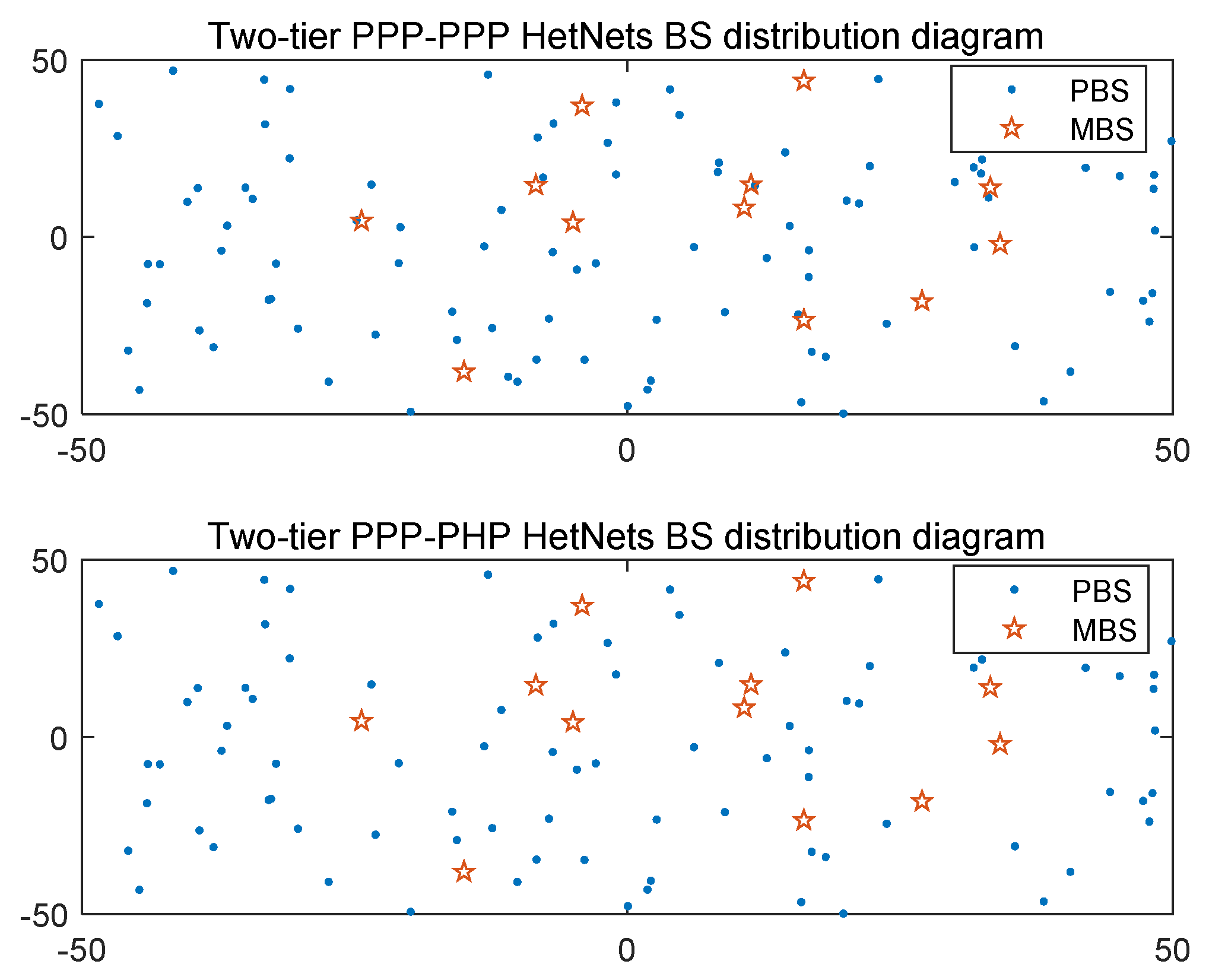
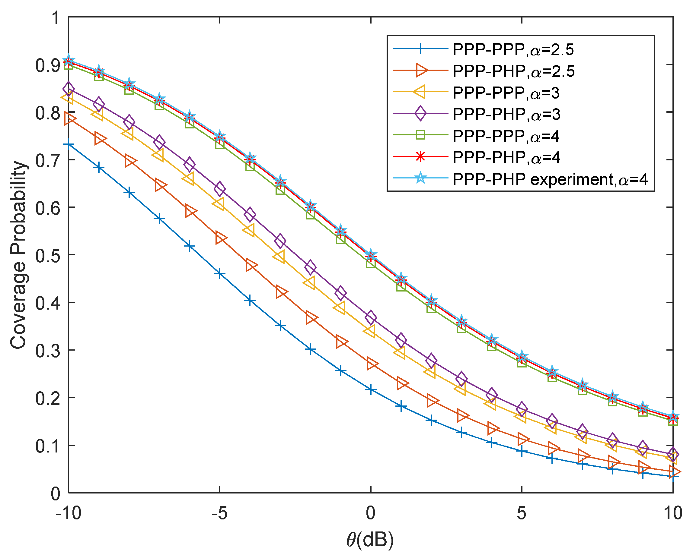
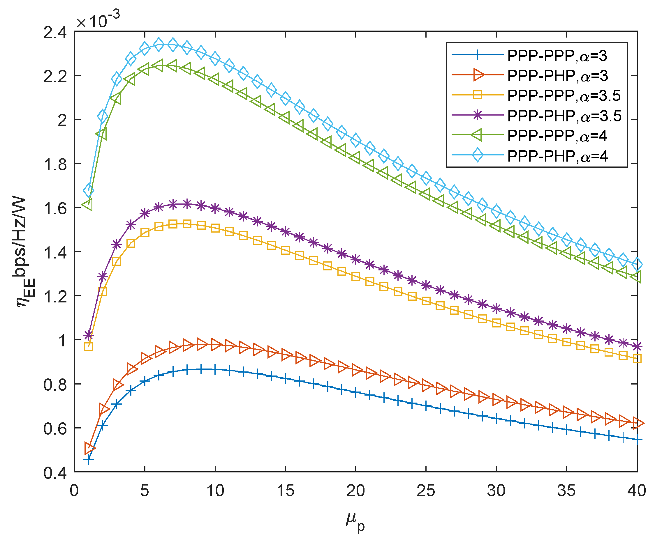
5. Simulation Results

In this section, we use the MATLAB software platform to simulate the performance of the two-tier PPP-PHP HetNets. The default simulation parameters of the system model are shown in

Table 2. Simulation parameters.

Parameter Symbol	Parameter Description	Parameter Value
${\lambda }_m$	Deployment density of the MBS	10−2 m−2
${\lambda }_p$	Deployment density of the PBS	0.1 m−2
$\theta$	Given threshold of the BS	0 dB
${\mu }_m$	MBS transmit power	40 W
${\mu }_p$	PBS transmit power	10 W
r	Repulsion radius	2 m
Pm0	MBS static power consumption	1000 W
Pp0	PBS static power consumption	50 W

. For the transmit power of the MBS and the PBS, we refer to the statistical data in [43].

Figure 3 gives the relationship between the coverage probability and the SIR threshold $\theta$ of the two-tier HetNets under different path loss factors. The coverage probability decreases with the increase in the SIR, because the coverage probability is defined as the probability that the SIR received by the user is greater than the threshold value. The higher the threshold value, the lower the probability, so the coverage probability also decreases accordingly. When $\alpha =4$, there is a slight gap between the simulation results of the coverage probability of the PPP-PHP HetNets and the corresponding theoretical deduction results. The gap is due to the approximate interference between the PHP distribution and the PPP distribution, which verifies the correctness of the MISR-based gain method. As seen from Figure 3, as the path loss factor increases, the coverage probability increases. As the path loss factor increases, the cumulative interference I₁ and I₂ decrease, the SIR_m and SIR_p increase, and the coverage probability also increases. Figure 3 also shows that the coverage probability of the PPP-PHP HetNets is larger than that of the PPP-PPP HetNets under the same path loss factor.

Figure 4 shows the relationship between the network energy efficiency and the PBS transmit power in different path loss factors. Figure 4 shows that the network energy efficiency first increases, and then decreases as the transmit power of the PBS increases. As the transmit power of the PBS increases, more users access the PBS and the power consumption of the PBS is small, causing the energy efficiency of HetNets to increase. When the number of users accessing the PBS reaches saturation, the continuous increase in the PBS transmit power will increase the total network power consumption and reduce the network energy efficiency. Therefore, we can trace an optimal PBS transmit power to obtain the maximum network EE. Figure 4 shows that, when the path loss factor is equal to 4, the network energy efficiency is greater than that under the other two path loss factors ($\alpha =3$ and $\alpha =3.5$); thus, there is no monotonic relationship between the network energy efficiency and the path loss factor, which provides an idea of how to optimize the EE from the perspective of the path loss factor.

Figure 5 shows the relationship between the EE of the two-tier HetNets and the SIR threshold in the cases of $\alpha =3.5$ and $\alpha =4$. The quadratic interpolation optimization algorithm is used to obtain the optimal transmit power of the PBS when $\alpha$ takes different values in the PPP-PPP HetNets and the PPP-PHP HetNets. The proposed algorithm is compared with the golden section method proposed in [43], as shown in

Table 3. Comparison of algorithm performance.

	Running Time	Iterates Times
The golden section method [43]	20.37 s	32
The quadratic interpolation algorithm	10.88 s	30

. When the optimal value of the PBS transmit power is obtained, the golden section method iterates 32 times and the running time is 20.37 s. The quadratic interpolation algorithm iterates 30 times and the running time is 10.88 s. The running time is related to the computer hardware configuration. From the simulation results, it can be seen that the quadratic interpolation algorithm has fewer iterations and faster convergence speed. When $\alpha =3.5$, the optimal transmit power allocations of the PBS corresponding to the two cellular networks are 7.60 W and 7.63 W, respectively. When $\alpha =4$, the optimal transmit power allocations of the PBS corresponding to the two cellular networks are 6.44 W and 6.46 W, respectively. In the PPP-PPP HetNets, for the two cases $\alpha =3.5$ and $\alpha =4$, when the PBS transmit power is optimal, the EE values of HetNets are 1.3% and 2.9% higher than when the PBS transmit power is fixed at 10 W, respectively. In the PPP-PHP HetNets, for $\alpha =3.5$ and $\alpha =4$, when the PBS transmit power is the optimal value, the EE values of HetNets are 1.25% and 2.8% higher than when the PBS transmit power is a fixed value of 10W, respectively. Therefore, the EE of HetNets can be improved by setting an appropriate PBS transmit power allocation. Whether $\alpha =3.5$ or $\alpha =4$, the EE of the two-tier PPP-PHP HetNets is higher than that of the PPP-PPP network.

6. Conclusions

This paper studies the performance of two-tier HetNets and improves the EE of HetNets by optimizing the PBS transmit power. First, the coverage probability and average achievable rate of the PPP-PHP HetNets are derived by the method based on the MISR, and the expression of the EE of HetNets is obtained according to the definition of EE. Then, an optimization algorithm, the quadratic interpolation method, is proposed to maximize the EE of HetNets by setting the appropriate PBS transmit power. Finally, the theoretical derivation and optimization algorithm are simulated and analyzed. The simulation results show that the transmit power of the PBS has a certain impact on the EE of HetNets, and the system EE can be effectively improved by optimizing the PBS transmit power. In addition, the PPP-PHP network is superior to the PPP-PPP network in both the coverage probability and EE. This paper only considers optimizing the PBS transmit power to improve the energy efficiency. Future work can improve the energy efficiency of the HetNets by jointly optimizing the transmit power of the PBS and the density of the PBS.

References

1. Khandekar, A.; Bhushan, N.; Ji, T.; Vanghi, V. LTE-Advanced: Heterogeneous Networks. In Proceedings of the 2010 European Wireless Conference (EW), Lucca, Italy, 12–15 April 2010. [Google Scholar]
2. Kim, R.Y.; Kwak, J.S.; Etemad, K. WiMAX Femtocell: Requirements, Challenges and Solutions. IEEE Commun. Mag. 2009, 47, 84–91. [Google Scholar] [CrossRef]
3. Andreev, S.; Petrov, V.; Dohler, M.; Yanikomeroglu, H. Future of Ultra-Dense Networks Beyond 5G: Harnessing Heterogeneous Moving Cells. IEEE Commun. Mag. 2019, 57, 86–92. [Google Scholar] [CrossRef] [Green Version]
4. Gao, M.J.; Li, J.; Jayakody, D.N.K.; Chen, H.; Li, Y.H.; Shi, J.L. A Super Base Station Architecture for Future Ultra-Dense Cellular Networks: Toward Low Latency and High Energy Efficiency. IEEE Commun. Mag. 2018, 56, 35–41. [Google Scholar] [CrossRef]
5. Wu, Y.; Qian, L.P.; Yang, X.; Zheng, J.; Shen, X. Dual-Connectivity Enabled Traffic Offloading via Small Cells Powered by Energy-Harvesting. In Proceedings of the IEEE Global Communications Conference, Singapore, 4–8 December 2017. [Google Scholar]
6. Zhu, X.; Shen, X.; Zeng, F.; Vincent, H.; Dong, W.; Chen, W.; Li, K. Spectrum Resource Sharing in Heterogeneous Vehicular Networks: A Noncooperative Game-Theoretic Approach with Correlated Equilibrium. IEEE Trans. Veh. Technol. 2018, 67, 9449–9458. [Google Scholar]
7. Slamnik, N.; Oki, A.; Muovi, J. Conceptual Radio Resource Management Approach in LTE Heterogeneous Networks using Small Cells Number Variation. In Proceedings of the IEEE XI International Symposium on Telecommunications, Sarajevo, Bosnia and Herzegovina, 24–26 October 2016. [Google Scholar]
8. Kure, E.H.H.; Engelstad, P.; Maharjan, S.; Gjessing, S.; Zhang, Y. Distributed Uplink Offloading for IoT in 5G Heterogeneous Networks under Private Information Constraints. IEEE Internet Things J. 2019, 6, 6151–6164. [Google Scholar] [CrossRef]
9. Vilgelm, M.; Linares, S.R.; Kellerer, W. Dynamic Binary Countdown for Massive IoT Random Access in Dense 5G Networks. IEEE Internet Things J. 2019, 6, 6896–6908. [Google Scholar] [CrossRef] [Green Version]
10. Wang, C.X.; Haider, F.; Gao, X.; You, X.H.; Yang, Y.; Yuan, D.; Aggoune, H.; Haas, H.; Fletcher, S.; Hepsaydir, E. Cellular Architecture and Key Technologies for 5G Wireless Communication Networks. IEEE Commun. Mag. 2014, 52, 122–130. [Google Scholar] [CrossRef] [Green Version]
11. Hossain, E.; Rasti, M.; Tabassum, H.; Abdelnasser, A. Evolution Toward 5G Multi-tier Cellular Wireless Networks: An Interference Management Perspective. IEEE Wirel. Commun. 2014, 21, 118–127. [Google Scholar] [CrossRef] [Green Version]
12. Li, Y.Z.; Zhang, Y.; Luo, K.; Jiang, T.; Li, Z.; Peng, W. Ultra-Dense HetNets Meet Big Data: Green Frameworks, Techniques, and Approaches. IEEE Commun. Mag. 2018, 56, 56–63. [Google Scholar] [CrossRef] [Green Version]
13. Wu, Y.; Qian, L.P.; Zheng, J.C.; Zhou, H.B.; Shen, X.S. Green-Oriented Traffic Offloading through Dual Connectivity in Future Heterogeneous Small Cell Networks. IEEE Commun. Mag. 2018, 56, 140–147. [Google Scholar] [CrossRef]
14. Chen, G.; Qiu, L.; Chen, Z. Area spectral efficiency analysis of multi-antenna networks modeled by Ginibre point process. IEEE Wirel. Commun. Lett. 2017, 7, 6–9. [Google Scholar] [CrossRef]
15. Zhou, Y. Simulation and Analysis of 5G Network Performance Based on Ginibre Point Process. Master’s Thesis, Shanghai Jiaotong University, Shanghai, China, 2019. [Google Scholar]
16. Chen, C.; Elliott, R.C.; Krzymien, W.A. Empirical distribution of nearest-transmitter distance in wireless networks modeled by Matérn hard core point processes. IEEE Trans. Veh. Technol. 2018, 67, 1740–1749. [Google Scholar] [CrossRef]
17. Wang, Y.; Zhu, Q. Modeling and analysis of small cells based on clustered stochastic geometry. IEEE Commun. Lett. 2017, 21, 576–579. [Google Scholar] [CrossRef]
18. Afshang, M.; Saha, C.; Dhillon, H.S. Nearest-neighbor and contact distance distributions for Matern cluster process. IEEE Commun. Lett. 2017, 21, 2686–2689. [Google Scholar] [CrossRef]
19. Afshang, M.; Dhillon, H.S. Poisson cluster process based analysis of HetNets with correlated user and base station locations. IEEE Trans. Wirel. Commun. 2018, 17, 2417–2431. [Google Scholar] [CrossRef]
20. Haenggi, M. User point processes in cellular networks. IEEE Wirel. Commun. Lett. 2017, 6, 258–261. [Google Scholar] [CrossRef]
21. Flint, I.; Kong, H.B.; Privault, N. Analysis of heterogeneous wireless networks using Poisson hard-core hole process. IEEE Trans. Wirel. Commun. 2017, 16, 7152–7167. [Google Scholar] [CrossRef]
22. Deng, N.; Zhou, W.; Haenggi, M. Heterogeneous cellular network models with dependence. IEEE J. Sel. Areas Commun. 2015, 33, 2167–2181. [Google Scholar] [CrossRef]
23. Haenggi, M. The mean interference-to-signal ratio and its key role in cellular and amorphous networks. IEEE Wirel. Commun. Lett. 2014, 3, 597–600. [Google Scholar] [CrossRef] [Green Version]
24. Ganti, R.K.; Haenggi, M. SIR asymptotics in general cellular network models. In Proceedings of the 2015 IEEE International Symposium on Information Theory (ISIT), Hong Kong, China, 14–19 June 2015. [Google Scholar]
25. Haenggi, M.; Ganti, R.K. Asymptotics and Approximation of the SIR distribution in general cellular networks. IEEE Trans. Wirel. Commun. 2016, 15, 2130–2143. [Google Scholar]
26. Adam, A.B.M.; Muthanna, M.S.A.; Muthanna, A.; Nguyen, T.N.; El-Latif, A.A.A. Toward Smart Traffic Management With 3D Placement Optimization in UAV-Assisted NOMA IIoT Networks. IEEE Trans. Intell. Transp. Syst. 2022, 1–11. [Google Scholar] [CrossRef]
27. Chaaf, A.; Muthanna, M.; Muthanna, A.; Alhelaly, S.; Elgendy, I.A.; Iliyasu, A.M.; El-Latif, A.A.A. Energy-Efficient Relay-Based Void Hole Prevention and Repair in Clustered Multi-AUV Underwater Wireless Sensor Network. Secur. Commun. Netw. 2021, 2021, 9969605. [Google Scholar] [CrossRef]
28. Rafiq, C.; Ping, W.; Min, W.; Muthanna, M.S.A. Fog Assisted 6TiSCH Tri-Layer Network Architecture for Adaptive Scheduling and Energy-Efficient Offloading Using Rank-Based Q-learning in Smart Industries. IEEE Sens. J. 2021, 21, 25489–25507. [Google Scholar] [CrossRef]
29. D’Andreagiovanni, F.; Mannino, C.; Sassano, A. GUB Covers and Power-Indexed Formulations for Wireless Network Design. Manag. Sci. 2013, 59, 142–156. [Google Scholar] [CrossRef] [Green Version]
30. Lorincz, J.; Matijevic, T. Energy-efficiency analyses of heterogeneous macro and micro base station sites. Comput. Electr. Eng. 2014, 40, 330–349. [Google Scholar] [CrossRef]
31. Arshad, M.W.; Vastberg, A.; Edler, T. Energy efficiency improvement through pico base stations for a green field operator. In Proceedings of the IEEE Wireless Communications and Networking Conference (WCNC), Paris, France, 1–4 April 2012. [Google Scholar]
32. Luo, Y.; Shi, Z.; Bu, F. Joint optimization of area spectral efficiency and energy efficiency for two-tier heterogeneous ultra-dense networks. IEEE Access 2019, 7, 12073–12086. [Google Scholar] [CrossRef]
33. Dong, X.; Zheng, F.C.; Zhu, X.; O’Farrell, T. On the Local Delay and Energy Efficiency of Clustered HetNets. IEEE Trans. Veh. Technol. 2019, 68, 2987–2999. [Google Scholar] [CrossRef]
34. Zhu, Q.; Wang, X.; Qian, Z.H. Energy-Efficient Small Cell Cooperation in Ultra-Dense Heterogeneous Networks. IEEE Commun. Lett. 2019, 23, 1648–1651. [Google Scholar] [CrossRef]
35. Lorincz, J.; Bogarelli, M. Heuristic approach for optimized energy savings in wireless access networks. In Proceedings of the 18th International Conference on Software, Telecommunications and computer networks (SoftCOM 2010), Dubrovnik, Croatia, 23–25 September 2010. [Google Scholar]
36. Lorincz, J.; Capone, A.; Begušić, D. Heuristic Algorithms for Optimization of Energy Consumption in Wireless Access Networks. KSII T Internet Inf. 2011, 5, 626–648. [Google Scholar] [CrossRef] [Green Version]
37. Lorincz, J.; Matijevic, T.; Petrovic, G. On interdependence among transmit and consumed power of macro base station technologies. Comput. Commun. 2014, 50, 10–28. [Google Scholar] [CrossRef]
38. Dataesatu, A.; Boonsrimuang, P.; Mori, K.; Boonsrimuang, P. Energy Efficiency Enhancement in 5G Heterogeneous Cellular Networks Using System Throughput Based Sleep Control Scheme. In Proceedings of the 22nd International Conference on Advanced Communication Technology (ICACT), Macau, China, 23–25 November 2020. [Google Scholar]
39. Li, Y.; Zhang, H.; Wang, J.; Cao, B.; Liu, Q.; Daneshmand, M. Energy-Efficient Deployment and Adaptive Sleeping in Heterogeneous Cellular Networks. IEEE Access 2019, 7, 35838–35850. [Google Scholar] [CrossRef]
40. Shuvo, M.S.A.; Munna, A.R.; Adhikary, T.; Razzaque, M. An Energy-Efficient Scheduling of Heterogeneous Network Cells in 5G. In Proceedings of the International Conference on Sustainable Technologies for Industry 4.0 (STI), Dhaka, Bangladesh, 24–25 December 2019. [Google Scholar]
41. Wang, Y.; Huang, C. Efficient management of interference and power by jointly configuring ABS and DRX in LTE-A HetNets. Comput. Netw. 2018, 150, 15–27. [Google Scholar] [CrossRef]
42. Tsiropoulou, E.E.; Katsinis, G.K.; Filios, A.; Papavassiliou, S. On the problem of optimal cell selection and uplink power control in open access multi-service two-tier femtocell networks. In Proceedings of the International Conference on Ad-hoc Networks & Wireless, Benidorm, Spain, 22–27 June 2014. [Google Scholar]
43. Yang, J.; Tan, Z.; Hu, H.; Chen, Y.H. Energy-efficient Microcell Base Station Power Control in Heterogeneous Cellular Network. In Proceedings of the IEEE International Conference Communication Technology, Chengdu, China, 27–30 October 2017. [Google Scholar]
44. Yang, J.; Pan, Z.; Xu, H.; Hu, H. Joint Optimization of Pico-Base-Station Density and Transmit Power for an Energy-Efficient Heterogeneous Cellular Network. Future Internet 2019, 11, 208. [Google Scholar] [CrossRef] [Green Version]
45. Chen, Y.H.; Guo, L.L.; Zhang, S.B. Energy efficiency optimization of heterogeneous cellular networks based on transmitting power of pico base station. J. Comput. Appl. 2020, 40, 1115–1118. [Google Scholar]
46. Haenggi, M. ASAPPP: A simple approximative analysis framework for heterogeneous cellular networks. In Proceedings of the Workshop on Heterogeneous Small Cell Networks (HetSNets’14), Austin, TX, USA, 12 December 2014; Available online: http://www3.nd.edu/~mhaenggi/talks/hetsnets14.pdf (accessed on 26 January 2023).
47. Bao, Z.Y.; Yang, J.; Hu, H. Analysis of SIR gain and approximate coverage of heterogeneous cellular networks based on Poisson hole process modeling. J. Nanjing Univ. Posts Telecommun. (Nat. Sci. Ed.) 2018, 38, 35–40. [Google Scholar]
48. Kendall, D.; Mecke, W.S.; Stoyan, J. Stochastic Geometry and Its Applications, 2nd ed.; Wiley: New York, NY, USA, 1995; pp. 25–58. [Google Scholar]
49. Jo, H.S.; Sang, Y.J.; Xia, P. Heterogeneous cellular networks with flexible cell association: A comprehensive downlink SINR analysis. IEEE Trans. Wirel. Commun. 2012, 11, 3484–3495. [Google Scholar] [CrossRef] [Green Version]
50. Hamdi, K.A. A useful lemma for capacity analysis of fading interference channels. IEEE Trans. Commun. 2010, 58, 411–416. [Google Scholar] [CrossRef]
51. Wei, H.; Deng, N.; Zhou, W. Approximate SIR analysis in general heterogeneous cellular networks. IEEE Trans. Commun. 2016, 64, 1259–1273. [Google Scholar] [CrossRef]
52. Dhillon, H.S.; Kountouris, M.; Andrews, J.G. Downlink MIMO hetNets: Modeling, ordering results and performance analysis. IEEE Trans. Wirel. Commun. 2013, 12, 5208–5222. [Google Scholar] [CrossRef] [Green Version]
53. Liao, L.F.; Ouyang, Z.Y. Beetle antennae search based on quadratic interpolation. Appl. Res. Comput. 2021, 38, 745–750. [Google Scholar]
Figure 1. Model of two-tier heterogeneous cellular network.
Futureinternet 15 00056 g001
Figure 2. Two-tier HetNets BS distribution diagram.
Futureinternet 15 00056 g002
Figure 3. Coverage probability versus SIR.
Futureinternet 15 00056 g003
Figure 4. Energy efficiency η E E versus the PBSs transmit power μ p under different α .
Futureinternet 15 00056 g004
Figure 5. Energy efficiency η E E versus SIR θ under different α .
Futureinternet 15 00056 g005