1. Introduction
While ensuring a stable and consistent user experience, the fifth-generation (5G) communication network provides ultra-high speed, low delay, ultra-reliability, and low-cost service quality, creating unprecedented new opportunities and convenience for society and the economy. Therefore, the large-scale commercialization of 5G networks is a current research hotspot in communication technology [
1]. In the field of wireless technology, massive Multiple-Input Multiple-Output (MIMO), millimeter-Wave (mmWave) technology, carrier aggregation technology, new multi-access access, and other technologies are important means to enhance the performance of 5G [
2]. In particular, massive MIMO systems can handle large network throughput and support a large number of client connections, which is expected to radically improve the capacity limitations of base stations and enable individual base stations to talk to more devices, thus driving the development of the Internet of Everything (IoE) [
3]. MmWave technology, which is higher than 4G radio frequency, can provide ultra-high speed and ultra-high spectral efficiency while reducing network connectivity costs [
4,
5]. These emerging 5G technologies can deliver a variety of extreme services more flexibly and reliably, supporting applications in various vertical industries to enable the IoE.
Even with the rapid development of wireless network technologies, IEEE 802.11 protocol-based network technology, as a reliable and economic information network construction method, is still considered a promising technology affecting the future communication industry and is also an important component of 5G and future wireless local area networks (WLANs). The transmission of emergency information and data with ultra-high reliability and low delay is one of the challenges faced by WLANs. Therefore, when numerous real-time emergency traffic is loaded on WLANs, it is necessary to provide it with a higher quality of service, which makes us think first of reducing the delay, so analyzing this parameter is a vital step to solving the problem [
6].
There have been many works on IEEE 802.11 network performance analysis and modeling [
2,
3,
4,
5,
6], but few works simultaneously consider the following factors to analyze the service delay of the medium access control (MAC) layer, such as the initial-carrier-sensing (ICS) procedure, the backoff counter freezing, up-to-date standard parameters, and computational complexity, etc. In [
7], Bianchi proposed a representative 2-D Markov model to analyze the saturated throughput of the IEEE 802.11 distribution coordination function (DCF). Afterward, based on the model of [
7], Ziouva et al. In [
8], the authors introduced the initial state before the node entered the backoff procedure and analyzed the throughput and delay of the 802.11 DCF. In [
9], the authors compared the proposed 2-D Markov model with a model that considered continuous packet transmission without activating the backoff procedure and demonstrated that the Markov model is more accurate in predicting the performance of the 802.11 protocol, obtaining the relationship between the data rate of the transmitted packets and the packet delay, packet discard time, and throughput. In [
10], the state of the channel when the buffer is idle is described, and the authors proposed a 2-D Markov model to analyze the throughput performance of the IEEE 802.11 MAC layer under non-ideal conditions. In [
11], the authors proposed a system model based on the 802.11 MAC protocol applicable to multiple contentions and proved that the stochastic evolution of different station backoff states converges to deterministic evolution in the limit state. The authors in [
12] analyzed an accurate MAC delay model, which considered the backoff counter decrementing time. Tadayon et al. [
13] proposed a service delay model to track the service delay behavior of 802.11 networks. The authors in [
14] studied the fair issue of access to the channel by vehicles with different speeds and its impact on the network throughput. All the above research works used the queueing theory approach or the Markov approach to model the performance of the 802.11 MAC layer. In addition, in [
15,
16,
17,
18], the use of machine learning methods (supervised learning [
15], reinforcement learning [
16], deep reinforcement learning [
17], joint learning [
18], etc.), which have been hotter in recent years, is proposed to study the performance of the MAC layer of 802.11 networks in terms of the throughput and channel utilization.
However, a great deal of research has been conducted on modeling the service delay of 802.11 networks. These studies generally conducted modeling in the form of non-closed expressions or individual statistical moments. For example, the authors in [
19] deduced the queuing delay and channel access delay of the 802.11 p DCF, but which were the non-closed model. In [
20], the author used the limiting probability,
, of successful transmission head-of-line (HOL) grouping to represent the saturated or unsaturated state of the network to study the performance of homogeneous cached IEEE 802.11 DCF networks, such as the delay, but the delay model was in the form of a single statistical moment. In [
21], the authors derived the access delay of the IEEE 802.11 DCF in the saturated state, as well as in [
22], where the authors derived the MAC delay and queuing delay using z-transform, which all investigated the mean, variance, and probability distributions of the MAC delay, but none of the resulting models could estimate the total delay spent in the transmitting packets. Furthermore, for the delay analysis of the point coordination function (PCF), see [
23,
24].
In this paper, we comprehensively consider four primary factors affecting the performance of IEEE 802.11 networks, including the ICS procedure, the backoff counter freezing, up-to-date standard parameters, and computational complexity, and constructed a novel statistical model for the service delay in 802.11 networks; it is a 2-D Markov model including the ICS procedure and the backoff procedure. The model can identify the service delay’s behavior and fully characterize the network performance. By analyzing the ICS delay and the backoff delay, we obtained the probability generating function (PGF) of the average idle time. The analytical expressions of the other service delays, such as the successful transmission time and collided transmission time, were derived to obtain the PGF of the total service delay. It was found that our delay evaluation results were significantly better than the traditional evaluation results. The average service delay of the Nav model in all the scenarios was larger than that of the analysis model due to the lack of the ICS procedure in the Nav model. Since a DIFS duration is generally much shorter than a random backoff duration, our model saves the bandwidth and improves transmission efficiency.
The rest of the paper is organized as follows. In
Section 2, we briefly analyze the transmission procedure of the IEEE 802.11 DCF mechanism and put forward the corresponding modeling ideas. In
Section 3, a 2-D Markov model is established to simulate the operating mechanism of the 802.11 DCF, and the transmission probability is obtained. In
Section 4, we calculate the average idle time experienced by a node between two consecutive successful transmissions. In
Section 5, we establish the total service delay model in the IEEE 802.11 network. In
Section 6, the validity and accuracy of the proposed model are verified by numerical simulation. Finally, the paper is concluded in
Section 7.
2. Analysis of IEEE 802.11 DCF Mechanism and Modeling Ideas
The basic operating principle of the 802.11 DCF mechanism is that the node should sense the channel activities before sending a data frame [
25]. The channel is usually busy or idle, so the node sensing channel activities are divided into two situations: (1) If the channel is sensed to be idle for a DCF interframe space (DIFS), the data frame will be sent. (2) If the channel is sensed to be busy, the node will continuously sense the channel until it becomes idle for a DIFS. At this moment, in order to avoid collisions as much as possible, the nodes will generate a random backoff interval that follows the binary exponential backoff algorithm. That is, when a node tries to transmit a data frame, the backoff timer (or the backoff counter) is uniformly chosen in the range of
, and the backoff window length in the
-th backoff stage is
,
. When the first attempt to send is made, the backoff window’s original length is
, and after each failed attempt to send, the backoff window length is two times that of the previous one until the maximum backoff stage is reached,
. During the backoff, whenever the node senses that the channel is idle for a slot time, the backoff counter is decremented by one, and the node cannot send data frames until it decrements to zero. It should be noted that nodes send data frames only at the beginning of each slot time, where the time slot length is the time required by any node to sense the farthest node transmission. Furthermore, the value of the DIFS can be expressed as
, where
,
, and
stand for the DIFS number, a time slot length, and a SIFS length, respectively.
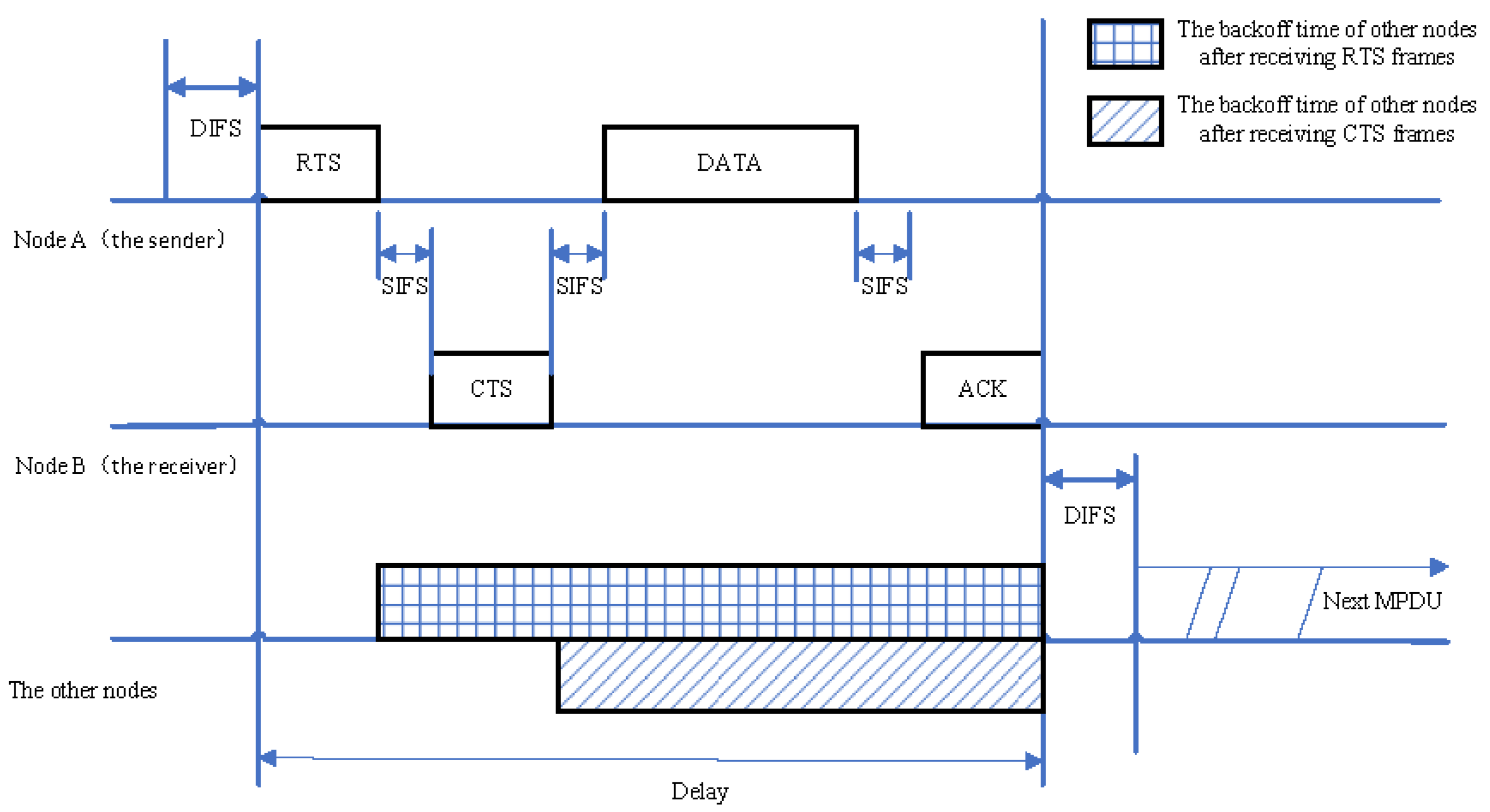
The DCF has two transmission modes [
26]. In the basic mode, after the data frame is sent, its successful reception is confirmed by the receiving node sending an acknowledgment (ACK) frame. Additionally, if no ACK frame is received, it will go through a backoff procedure and start to retransmit. This mode does not solve the problem of conflicts that may be caused by hidden nodes. However, the ready-to-send (RTS)/clear-to-send (CTS) transmission mode avoids the conflicts caused by the hidden nodes during transmission [
11]. Its main principle is to control the transmission status of the node (transmitting data or in the backoff procedure) using the transmitting data frames’ information carried by the RTS/CTS frames. Therefore, we mainly discuss the RTS/CTS transmission mode. The main feature of this mode is that before sending data frames to the receiving node B, the sending node A must send the RTS frames to make a reservation channel and to inform the other nodes, except node B, to postpone sending while node B will send the CTS frames to node A after receiving the RTS frames. The specific transmission process is shown in
Figure 1.
In order to describe the service delay’s behavior more accurately in real WLANs, different from existing research, this paper comprehensively considers the following four major factors to build a system model:
ICS procedure: If a new data frame arrives when the channel is idle, the frame will start the ICS procedure, i.e., if the channel is idle for a DIFS, the data frame will be transmitted immediately at the end of the DIFS without entering the backoff procedure. Otherwise, if the channel is detected to be busy during the DIFS, the data frame will enter the backoff procedure;
Backoff counter freezing: When the channel is sensed to be busy, the backoff counter will pause its decrementing process. Once the channel is sensed to be idle, the backoff counter will be activated again to continue its decrement procedure;
Up-to-date standard parameters: to make our model suitable for the real network environment, some parameters need to be updated, including the DIFS, SIFS, time slot length, retransmission limit, and contention window size, and so on;
Computational complexity: In order to solve the problem more clearly and simply, the model should minimize the complexity of the calculation. Therefore, the transmission model considers a 2-D Markov model, and to verify the model’s accuracy, we only need to focus on the first two statistical moments of the service delay model.
3. Markov Modeling Analysis of IEEE 802.11 Operations
In this section, we will improve the model by adding the ICS procedure based on the Bianchi model [
7]. i.e., if the node senses that the previous data frame has been successfully received and the channel is idle for a DIFS, the node will directly send a new data frame, which the process of the new data frame waits for sending is called the ICS procedure.
As shown in
Table 1, to further illustrate the difference between the proposed model and the original Bianchi model, we briefly summarize it, and we assume that after the node successfully transmits the previous frame, the node has a new data frame waiting to be sent (the successful transmission of the previous data frame can be seen in
Figure 1). Obviously, the proposed model does not need to enter the backoff procedure after successfully transmitting the previous frame but directly starts the ICS procedure, which greatly reduces the idle time of the channel. This work can not only reduce the service delay of the network but also reduces the waste of the bandwidth so as to improve the network throughput and channel utilization. In particular, a low delay and high throughput are the desired goals when the network is loaded with large amounts of emergency traffic.
Next, we assume that the channel condition is a single-cell environment with terminals. The channel has no defects, i.e., the data frames’ collision (probability ) is the only factor that causes transmission errors. Furthermore, the terminal is always in three states, i.e., the transmission, ICS, or backoff procedure.
Letting denote the state of the transmit queue at time , we can obtain:
the backoff state, , where denotes the value of the backoff stage, and is the value of the backoff counter of the data frame at the head-of-line (HOL);
The ICS state, , where , and is a time slot length. The state means that the channel is sensed to be idle for the period during the ICS procedure;
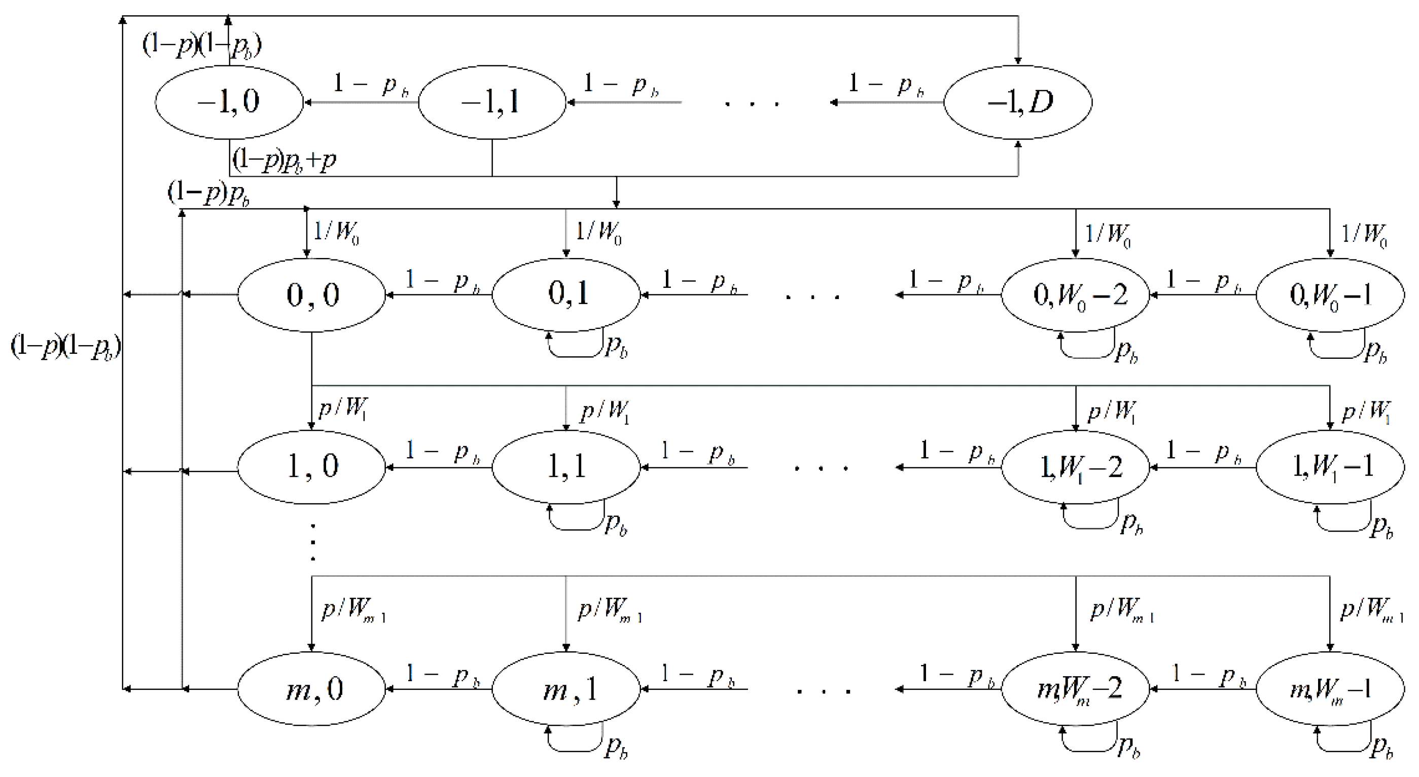
Next, we obtain the state transition diagram (
Figure 2) of the 2-D Markov chain, which considers all the major factors. The corresponding one-step transition probabilities are as follows (where
is the probability that the channel is busy):
if the HOL data frame is successfully transmitted, start the backoff procedure:
If the HOL data frame is unsuccessfully transmitted, the frame is retransmitted, resulting in an increase in the backoff stage:
If the HOL data frame is successfully transmitted and the channel is sensed to be idle for a DIFS, the ICS procedure is initiated:
- 2.
For the case of during the ICS procedure:
if the channel is sensed to be idle for a time slot, the counter decreases by one:
If the channel is sensed to be busy, the backoff procedure is initiated:
- 3.
For the case of during the ICS procedure:
after the node successfully transmits the previous data frame, it senses that the channel is idle for a DIFS and continues the ICS procedure:
If the transmitted HOL frame encounters a collision, it enters the 0-backoff stage, or if the channel is sensed to be busy after successfully transmitting the frame:
- 4.
In order to represent the backoff counter freezing, for :
the backoff counter freezes when the node senses that the channel is busy:
If the channel is sensed to be idle, the counter is decremented by one:
Then, set the probability of the collision during the data frame transmission as
, and denote the steady-state probability distribution of the system
as follows:
Under the steady-state condition of the system, we have the following steady-state equations:
From the probability normalization,
, and Equations (10)–(13), we can obtain:
According to Equations (10)–(14), we obtain the steady-state probability distribution. Define
as the probability that a node transmits in a time slot, i.e., the steady-state probability when a node is in the backoff stage,
(
), and the backoff counter is
, or the ICS procedure ends. Therefore, it holds that:
Substituting Equations (10) and (14) into the above equation, we obtain:
4. Calculation of the Average Idle Time
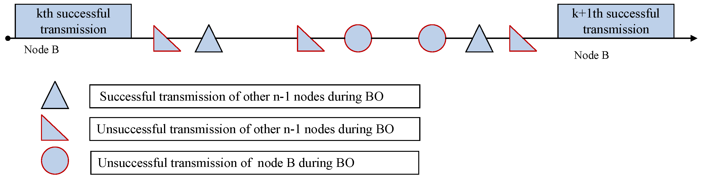
Based on the above Equation (15), we will calculate the average idle time from the perspective of observer node B, as shown in
Figure 3. Note that the value
of the backoff counter decreases in units of
when node B detects that the channel is idle, with a probability of
. The counter is frozen when node B detects that the channel is busy with the probability,
, and only when the counter’s value is decremented from
to
will the node successfully transmit with the probability,
. When the backoff stage reaches the maximum (or retransmission limit), the data frame still fails to transmit, i.e.,
, and the frame will be discarded immediately. Therefore, the following correlation probabilities were found:
The collision probability, , i.e., the probability that at least one of the remaining competing nodes at a time slot sends a data frame, can be found as ;
The probability that the channel is busy, i.e., the probability that at least one node transmits at a time slot, can be found as ;
Since the channel has no defects, the total collision probability, , is only related to the busy channel caused by the data frame transmission and data frames’ collision, and it can be expressed as ;
The successful transmission probability, , i.e., under the condition that at least one node of the nodes transmits at a time slot, the probability that exactly one node transmits successfully can be expressed as .
Based on the above analysis, we note that the time interval between the two consecutive successful transmissions of node B (
-th and
-th in
Figure 3) may include events, such as failure of sending data frames by node B, the other
nodes successfully send data frames or fail to send data frames when B carries out the backoff procedure, and the channel is idle. Thus, the average idle time,
, experienced by node B between two consecutive successful transmissions is defined as the average time that the ICS procedure was performed and the average time that the backoff counter was active during the backoff procedure. From this, it can be determined that the expression of
is:
The first term of Equation (16) is the average idle time to complete the ICS procedure, denoted as . The second item is the average idle time that the node may traverse, which performs the backoff procedure after the channel is sensed to be busy during the ICS procedure. Note that follows a uniform distribution, with a mean of . Therefore, starting from the second term, it describes the average idle time of the backoff procedure, denoted as , where is a random variable subject to a uniform distribution and is the original length of the backoff counter at each retransmission attempt, and and are independent of each other.
Let the probability generation function (PGF) of
be
, and use the properties of PGF to obtain:
where
. The above equation will be used to derive our modeling.
5. Service Delay Statistical Model
In this section, the total service delay in 802.11 networks is analyzed to obtain its PGF. We define service delay as the period from the time when the data frame arrives at the HOL of the sending node to the time when it is successfully received by the receiving node. During this period, a node may detect or go through different channel activities, such as whether the node succeeded or failed in sending the data frames and the success or failure of the other
nodes to send data frames and channel leisure [
13].
Let
,
,
,
, and
denote the time when node B successfully transmits a data frame, the node B transmission collision time, the time when the other
nodes successfully transmit the data frames, the other
nodes transmission collision times, and the channel’s idle duration, respectively. Then, the service delay,
, can be expressed as:
where
,
, and
denote the number of node B retransmissions and the number of collided transmissions and successful transmissions for the other
nodes during
, respectively. Regarding them, the following conclusions hold:
Conclusion 1: The number of a node retransmissions,, obeys a truncated geometric distribution. Thus, Conclusion 2: If the B node has successfully completed its-th transmission and started the backoff procedure, thenodes are trying to access the channel at this time. Theevents andsuccessful transmissions occur for the remainingnodes, attempting to access the channel during the node B backoff period. Let the random variabledenote the number of times that the remainingnodes attempt to send a data frame before node B successfully transmits its-th data frame. Then,obeys the conditional probability distribution:where. Conclusion 3: Define, i.e., the number of collisions that occur when the remainingattempt to send the data frames before the node makes the-th successful transmission. Then, the conditional probability distribution ofis: The following analyzes
. We find that there must be only busy or idle events in the time period between two consecutive transmissions of a node, and the two events occur alternately in the 802.11 DCF protocol. The length of time of each idle or busy event that occurs depends on the size of the transmitted data frame and the opportunity of the node to transmit the data frame, etc., while the average time for idle events to occur is:
Due to channel idle events occurring independently, it obeys the geometric distribution of parameter
. Let
represent the number of idle events (counted in a slot time), then:
Furthermore, since the busy or idle state of the channel in the DCF protocol takes place alternately successively over time, it is impossible for the idle or busy to occur twice in succession. Therefore, the number of idle events during
can be approximately equal to the number of busy events (counted in a slot time),
, and namely,
. Since the occurrence of the busy events is caused by the successful transmission of the data frames or data frame transmission collision,
is divided into two parts, namely the number of busy events due to the successful sending of the data frames,
, and the number of busy events due to the data frame transmission conflicts,
. Therefore,
For the last term,
, the idle time in (18), since the backoff counter is frozen when the channel is busy, can be expressed as
minus the number of busy slots,
, i.e.,
. In addition, since
,
, and
are independent random variables, the PGF of
can be obtained by applying
-transformation to Equation (18), as follows:
Combining the above results, using the properties of the conditional PGF [
27], we can obtain:
where
,
So far, we obtain a closed expression for the PGF of the service delay
by Formulas (25)–(29). Since all the protocol details have been considered in the discussion, the PGF can reasonably describe the service delay behavior of the 802.11 network. Furthermore, we obtain the mean and the variance of
by the first-order derivative and second-order derivative, i.e.,
6. Numerical Simulation
In this section, the numerical simulation results are given to verify the validity of the proposed analysis model. As mentioned above,
,
,
,
,
, and
represent the minimum contention window size, the number of contending nodes, the maximum backoff stage (or retransmission limit), collision probability, and the time when a node successfully transmits a data frame and transmission collision time, respectively. The time when a node successfully transmits a data frame and transmission collision time depends on two transmission modes, i.e., one is the RTC/CTS mode,
,
, and the other is the basic mode,
and
. Using the above parameters, we consider three transmission scenarios (as shown in
Table 2), and the parameter settings of each scenario are from [
13]. That is, exactly one set of data is taken for each of the three different scenarios set in [
13] to achieve the goal of ensuring that the proposed model is valid over a wide range of parameters while also avoiding the complexity of the simulation process.
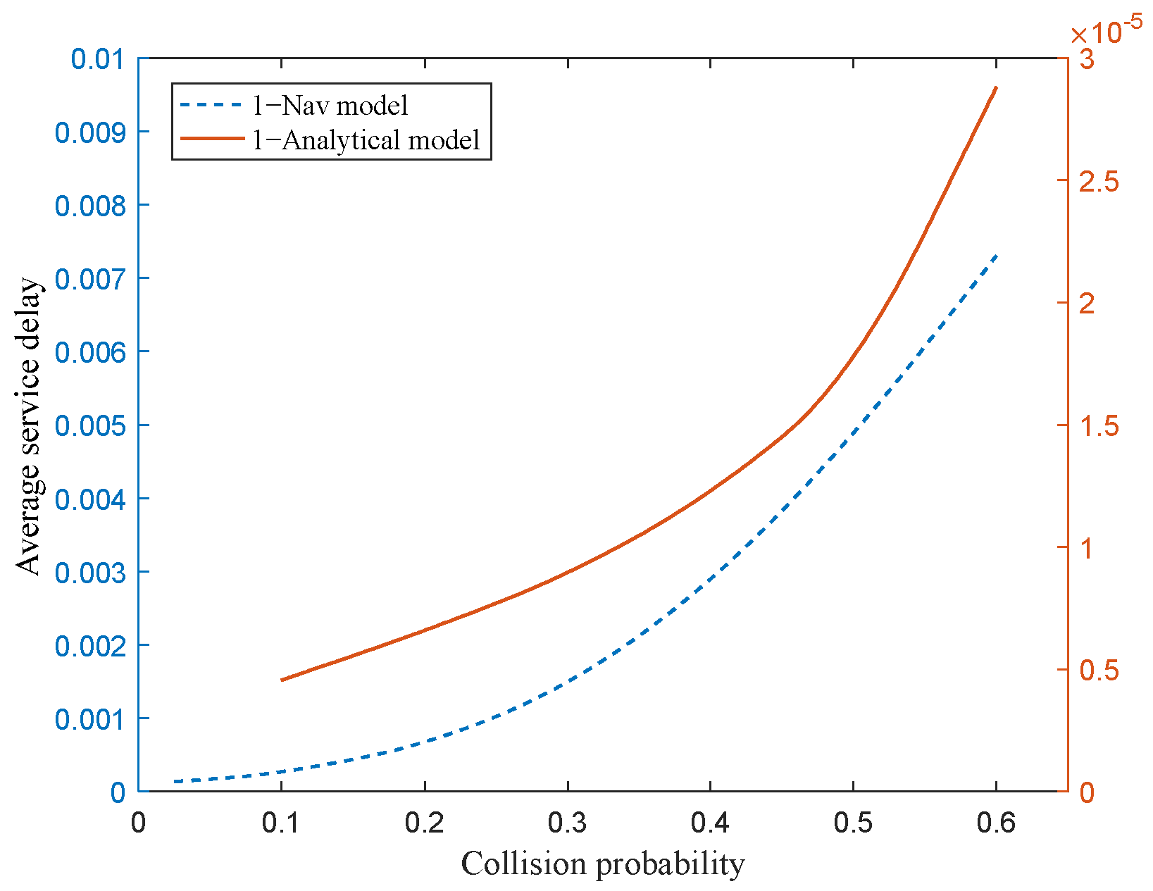
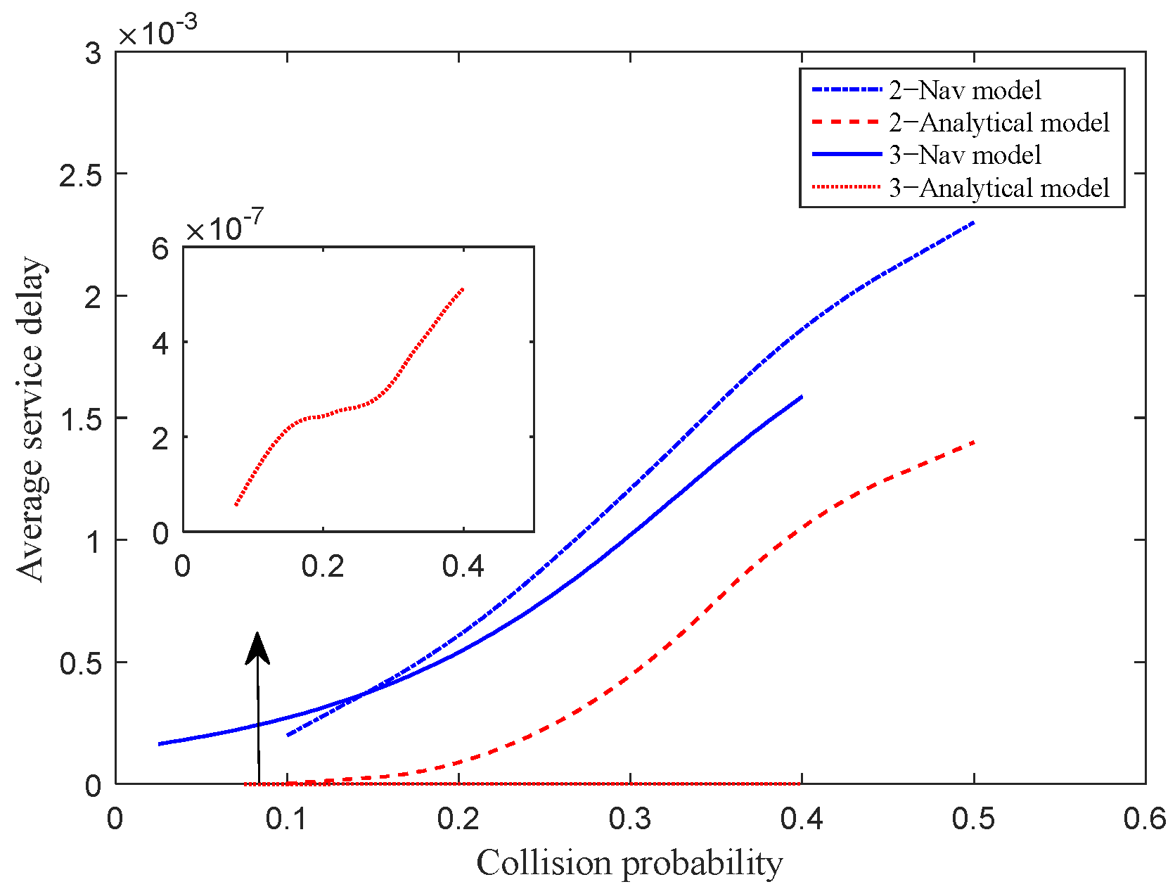
Figure 4 and
Figure 5 show the functional relationship between the average service delay and collision probability,
, in all the scenarios, where
Figure 4 is in Scenario 1, and
Figure 5 is in Scenario 2 and Scenario 3. Obviously, the average service delay of the Nav model in all the scenarios is bigger than that of the analysis model due to missing the lack of the ICS procedure in the Nav model. For the ICS procedure, after the previous data frame is successfully sent, the new data frame can be sent directly after the channel is idle for a DIFS, which further effectively reduces the service delay. Furthermore, the phenomenon in
Figure 4 that the average service delay of the analysis model is much smaller than that of the Nav model could indicate that the RTS/CTS mode has advantages over the basic mode.
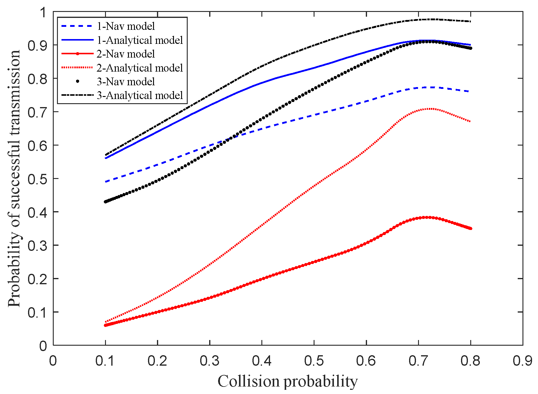
In
Figure 6, we obtain the comparison graphs of the successful transmission probability,
, between the analysis model and the Nav model in three scenarios. The following is a brief explanation, with Scenario 2 as an example. We can observe that as the collision probability increases, the successful transmission probability of our model is much larger than that of the Nav model because it comprises the ICS procedure. Indeed, since a DIFS duration is generally much shorter than a random backoff duration, our model saves the bandwidth and improves the transmission efficiency.
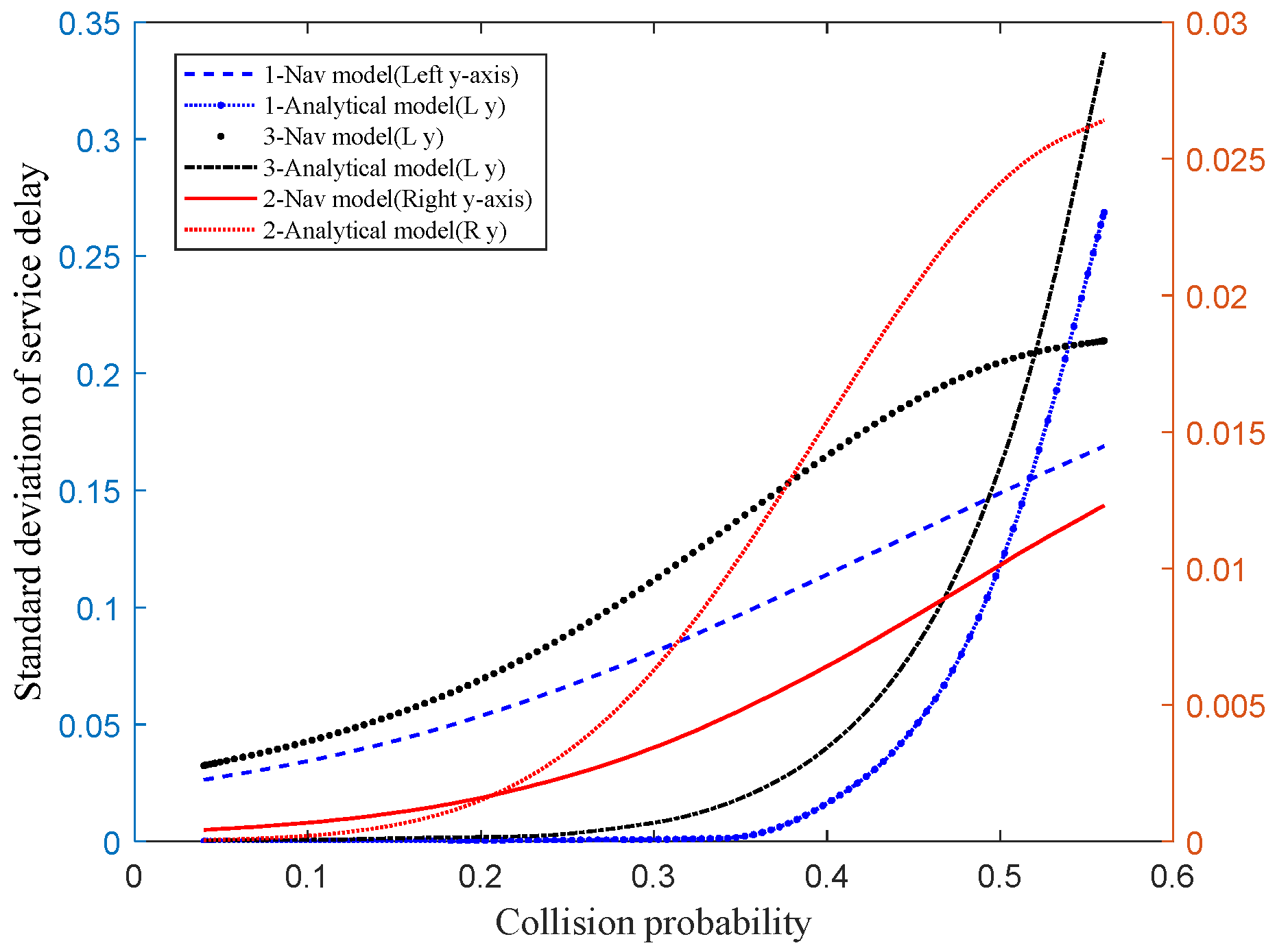
Figure 7 shows the standard deviation of the service delay in terms of the collision probability in all the scenarios. In any scenario, when the collision probability is smaller, the standard deviation of the service delay for the analysis model is smaller than that of the Nav model. That is because the ICS procedure added to the analysis model saves the transmission delay. When the collision probability reaches a certain value, the standard deviation of the service delay for our model is much larger than that of the Nav model. That is because the duration of the ICS procedure is much smaller than the backoff procedure. Thus, as the collision probability increases, the service delay of the analysis model is bigger as the frequency of entering the backoff procedure increases, and the gap of the service delay standard deviations is larger.


