

A Mechanistic Pharmacodynamic Modeling Framework for the Assessment and Optimization of Proteolysis Targeting Chimeras (PROTACs)

Abstract
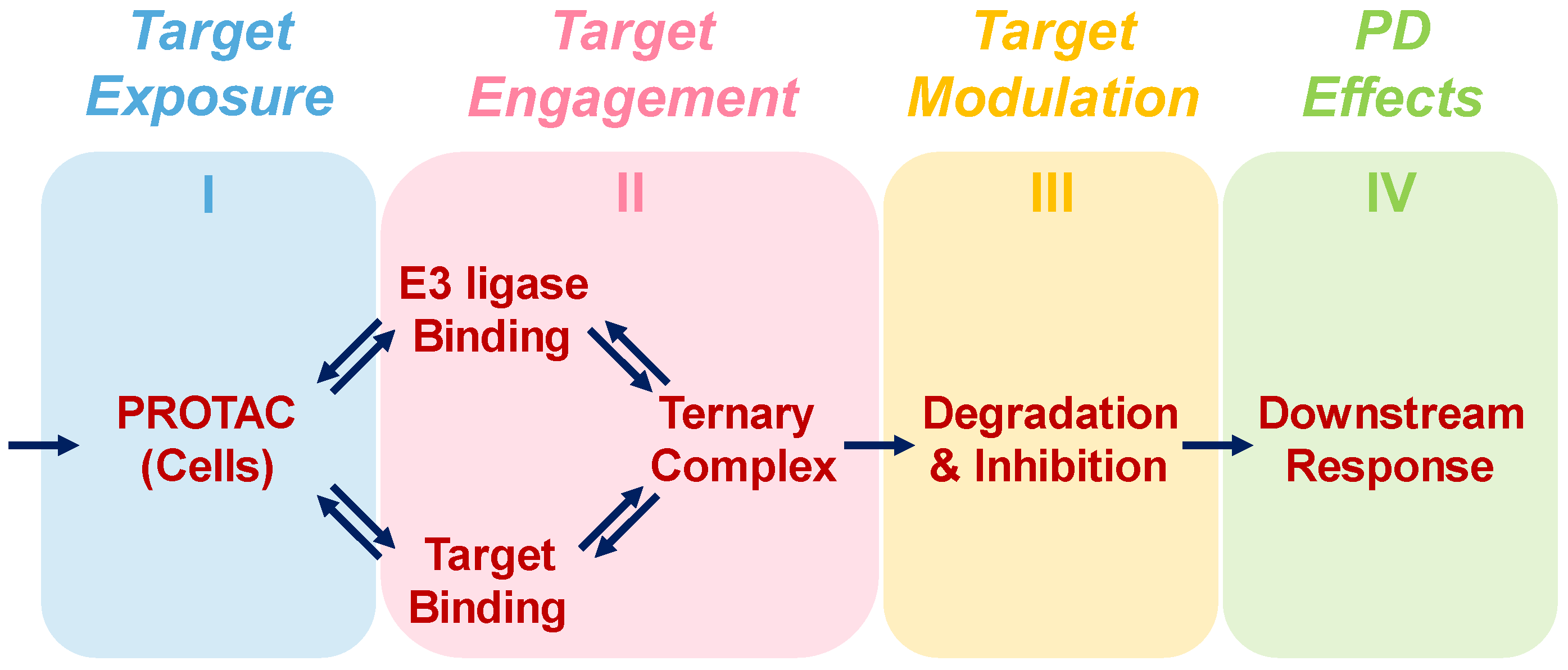
:1. Introduction
2. Materials and Methods
2.1. Modeling Approach
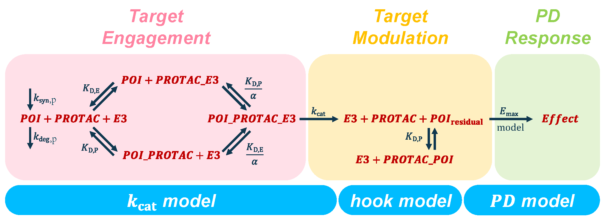
2.2. Pillar II—Target Engagement
2.3. Pillar III—Target Modulation
2.4. Pillar III.a—Target Degradation
2.5. Pillar III.b—Target Inhibition
2.6. Pillar IV—Pharmacodynamic Effects
2.7. Practical Application
- How much degradation is there? → hook model
- How to increase the extent of degradation? → model
- How much degradation is necessary? → PD model
3. Results
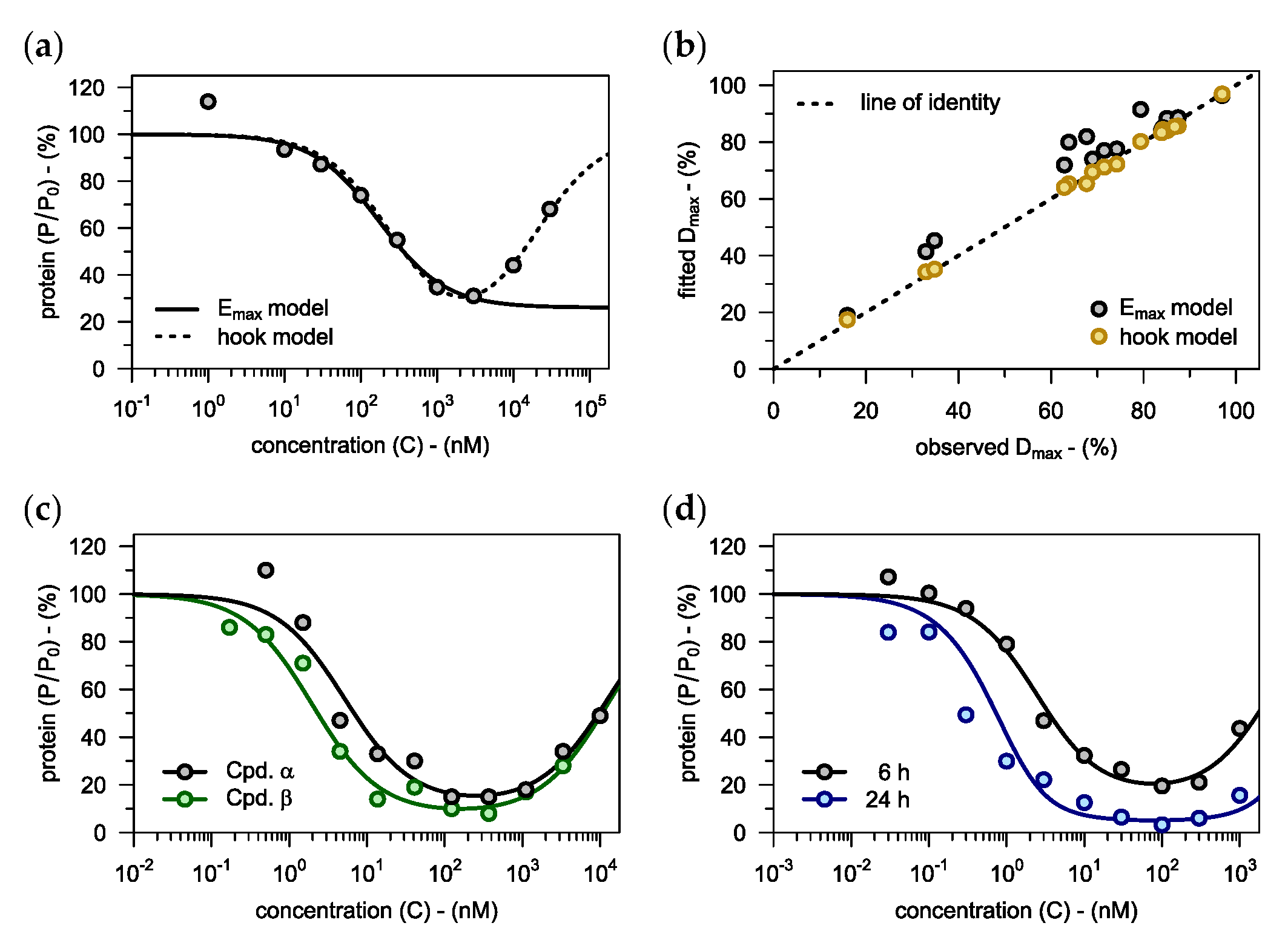
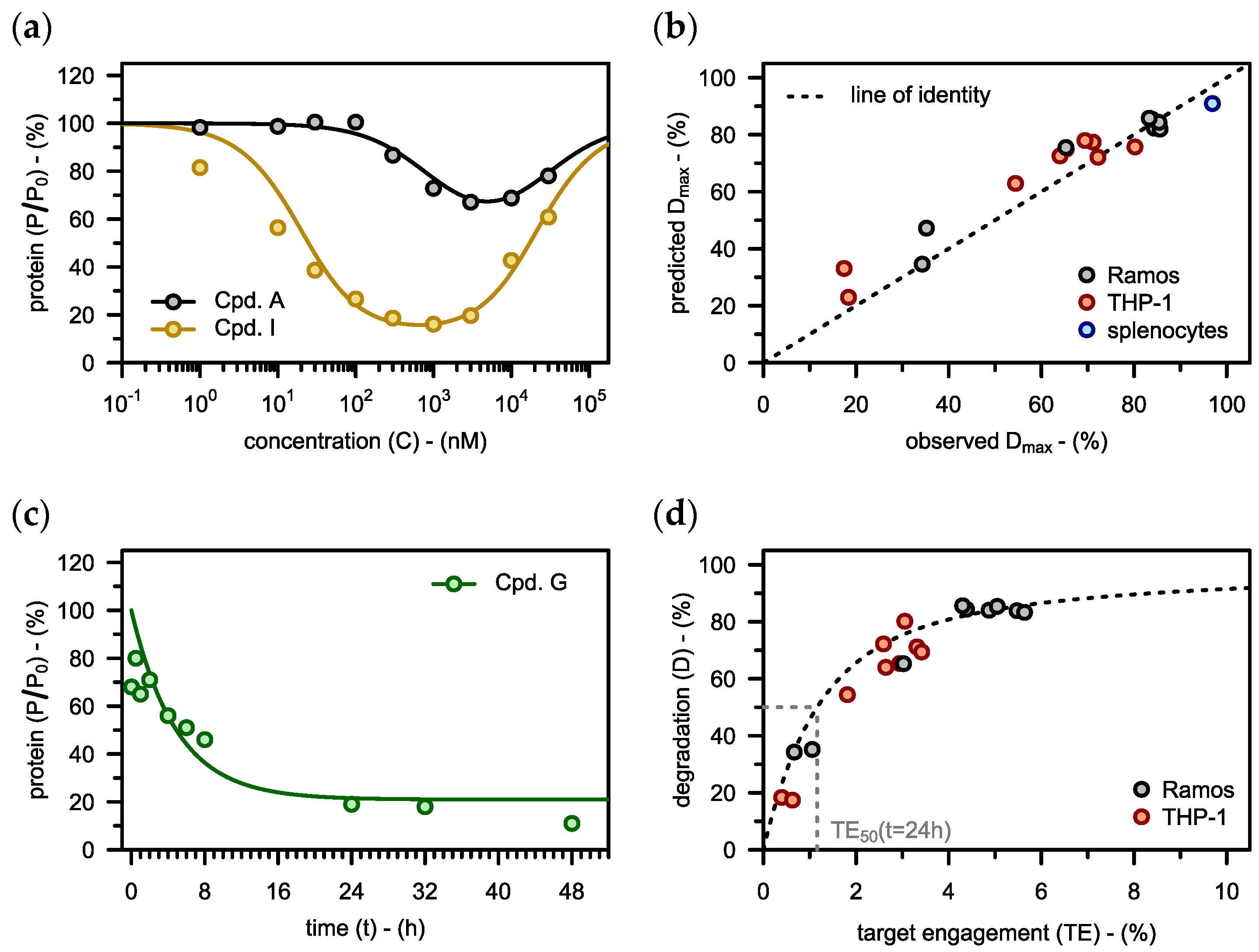
3.1. Assessing PROTACs as Degraders
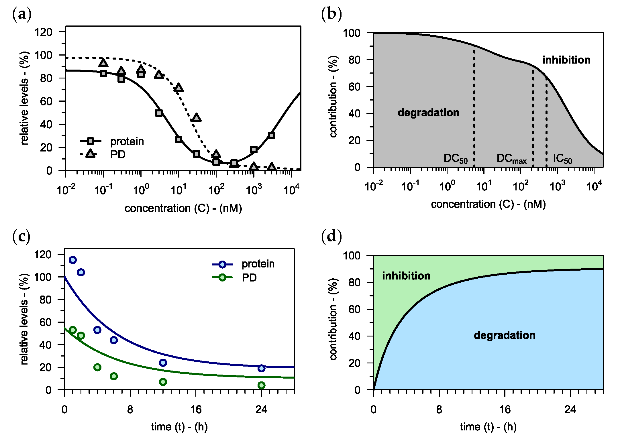
3.1.1. Capturing the Hook Effect
3.1.2. Impact of Incubation Time
3.2. Model-Informed Optimization of PROTACs
3.2.1. Binding Affinities
3.2.2. Physiological Parameters
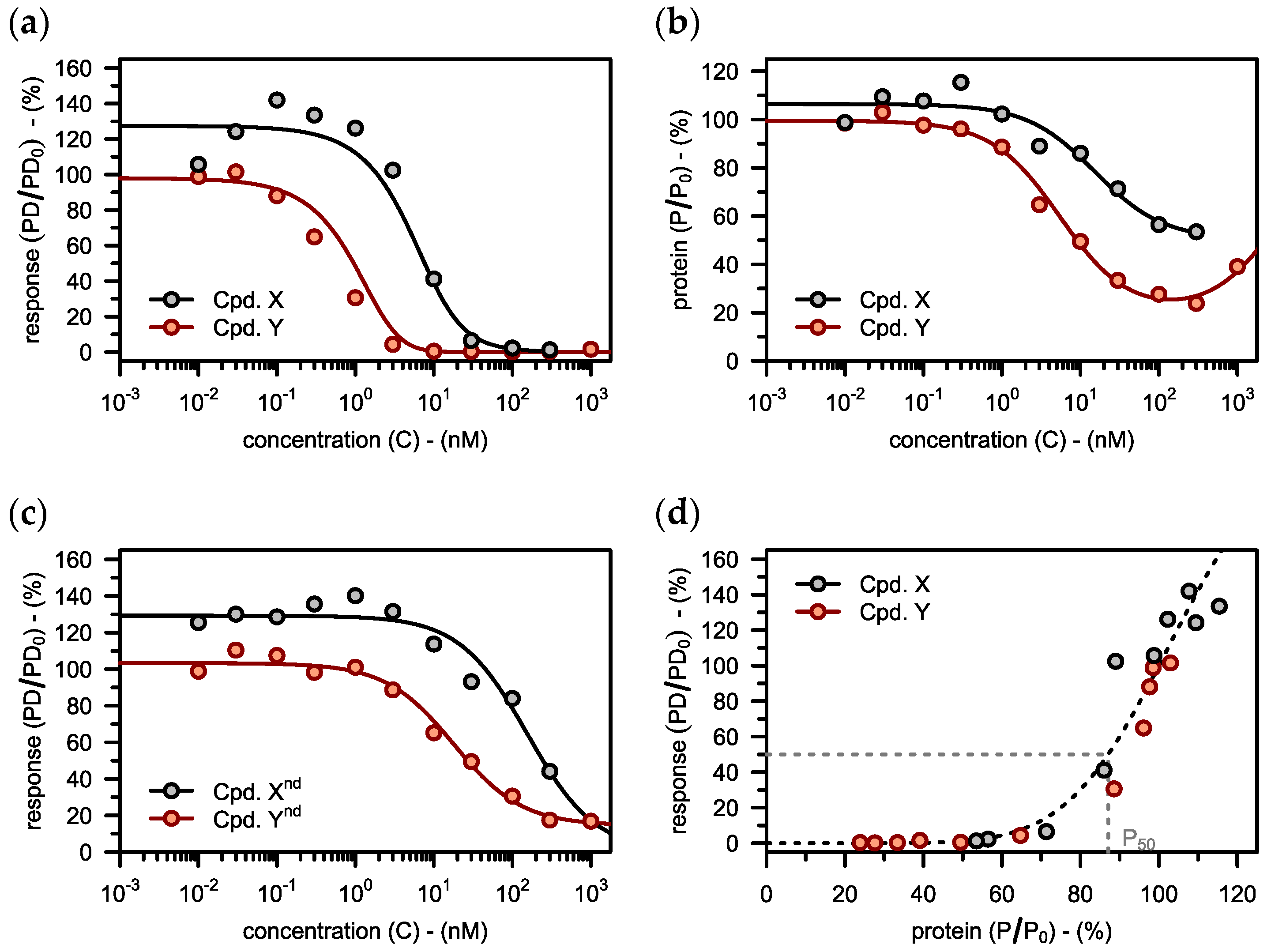
3.3. Deriving a Target Value for Degradation
3.3.1. Linking Degradation to the Pharmacodynamic Response
3.3.2. Interplay of Degradation and Inhibition
4. Discussion
4.1. The Hook Model
4.1.1. Advancing Current Best Practices
4.1.2. Guidance for Experimental Design
- (I)
- Use of an incubation time that is long enough to directly yield the steady-state profile. However, the required incubation time will be different for different PROTAC concentrations [19]. Therefore, one cannot conclude that the steady state has been reached just because degradation at a particular concentration is the same over time. Instead, we propose a different approach that requires only rough estimates for protein half-life () and for the maximal extent of degradation () as inputs. A threshold value for the minimal extent of degradation that is still acceptable is defined first (e.g., ). Next, the protein’s half-life or at least a rough estimate that should rather be too high than too low must be approximated. From these parameters, minimum required incubation times for in vitro degradation experiments can be calculated (see Table 2).
- (II)
- If target protein half-life is longer than 24 h, the theoretically required incubation times exceed what is practically feasible. For such cases, the extended hook model (Equation (14)) allows to estimate steady-state parameters from a pre-steady-state concentration-degradation profile obtained with standard incubation times. Yet, this second approach using the extended hook model (Equation (14)) is also more sensitive to measurement errors and requires precise estimates for protein half-life. These may be obtained by fitting concentration-degradation profiles at different incubation times in parallel.
- (Ⅲ)
- Finally, the question remains, which drug concentrations to study in vitro. To get the most reliable parameter estimates, one should cover the entire profile, including concentrations of no degradation up to concentrations displaying the hook effect. Demonstrating that there is a hook effect in protein degradation also is strong evidence in favor of the PROTAC mechanism of action. If no prior information about the relevant concentration range is available upfront, one could estimate from the binary binding affinities (see Appendix B) to get an initial idea. However, assay artefacts might occur more frequently at the highest concentrations, if for instance compounds become cytotoxic or poorly dissolved.
4.2. The Model
4.2.1. Lessons Learnt about the PROTAC Mechanism of Action
4.2.2. Model-Informed Drug Discovery
4.3. The Model
4.3.1. Leveraging the Inhibitory Activity of PROTACs
4.3.2. Model-Informed Target Validation
5. Conclusions
Supplementary Materials
Author Contributions
Funding
Institutional Review Board Statement
Informed Consent Statement
Data Availability Statement
Acknowledgments
Conflicts of Interest
Appendix A
Appendix B
Appendix C
Appendix D
References
- Li, K.; Crews, C.M. PROTACs: Past, Present and Future. Chem. Soc. Rev. 2022, 51, 5214–5236. [Google Scholar] [CrossRef] [PubMed]
- Lai, A.C.; Crews, C.M. Induced Protein Degradation: An Emerging Drug Discovery Paradigm. Nat. Rev. Drug Discov. 2017, 16, 101–114. [Google Scholar] [CrossRef] [PubMed] [Green Version]
- Luh, L.M.; Scheib, U.; Juenemann, K.; Wortmann, L.; Brands, M.; Cromm, P.M. Prey for the Proteasome: Targeted Protein Degradation—A Medicinal Chemist’s Perspective. Angew. Chem. Int. Ed. Engl. 2020, 59, 15448–15466. [Google Scholar] [CrossRef] [PubMed]
- Xiao, M.; Zhao, J.; Wang, Q.; Liu, J.; Ma, L. Recent Advances of Degradation Technologies Based on PROTAC Mechanism. Biomolecules 2022, 12, 1257. [Google Scholar] [CrossRef] [PubMed]
- Békés, M.; Langley, D.R.; Crews, C.M. PROTAC Targeted Protein Degraders: The Past is Prologue. Nat. Rev. Drug Discov. 2022, 21, 181–200. [Google Scholar] [CrossRef] [PubMed]
- Han, B. A Suite of Mathematical Solutions to Describe Ternary Complex Formation and their Application to Targeted Protein Degradation by Heterobifunctional Ligands. J. Biol. Chem. 2020, 295, 15280–15291. [Google Scholar] [CrossRef]
- Douglass, E.F., Jr.; Miller, C.J.; Sparer, G.; Shapiro, H.; Spiegel, D.A. A Comprehensive Mathematical Model for Three-Body Binding Equilibria. J. Am. Chem. Soc. 2013, 135, 6092–6099. [Google Scholar] [CrossRef] [Green Version]
- Bartlett, D.W.; Gilbert, A.M. A Kinetic Proofreading Model for Bispecific Protein Degraders. J. Pharmacokinet. Pharmacodyn. 2021, 48, 149–163. [Google Scholar] [CrossRef]
- Lesko, L.J. Perspective on Model-Informed Drug Development. CPT Pharmacomet. Syst. Pharmacol. 2021, 10, 1127–1129. [Google Scholar] [CrossRef]
- Marshall, S.; Madabushi, R.; Manolis, E.; Krudys, K.; Staab, A.; Dykstra, K.; Visser, S.A.G. Model-Informed Drug Discovery and Development: Current Industry Good Practice and Regulatory Expectations and Future Perspectives. CPT Pharmacomet. Syst. Pharmacol. 2019, 8, 87–96. [Google Scholar] [CrossRef]
- Visser, S.A.G.; Aurell, M.; Jones, R.D.O.; Schuck, V.J.A.; Egnell, A.C.; Peters, S.A.; Brynne, L.; Yates, J.W.T.; Jansson-Löfmark, R.; Tan, B.; et al. Model-Based Drug Discovery: Implementation and Impact. Drug Discov. Today 2013, 18, 764–775. [Google Scholar] [CrossRef] [PubMed]
- Nowak, R.P.; Jones, L.H. Target Validation Using PROTACs: Applying the Four Pillars Framework. SLAS Discov. 2021, 26, 474–483. [Google Scholar] [CrossRef] [PubMed]
- Pike, A.; Williamson, B.; Harlfinger, S.; Martin, S.; McGinnity, D.F. Optimising Proteolysis-Targeting Chimeras (PROTACs) for Oral Drug Delivery: A Drug Metabolism and Pharmacokinetics Perspective. Drug Discov. Today 2020, 25, 1793–1800. [Google Scholar] [CrossRef] [PubMed]
- Cantrill, C.; Chaturvedi, P.; Rynn, C.; Petrig Schaffland, J.; Walter, I.; Wittwer, M.B. Fundamental Aspects of DMPK Optimization of Targeted Protein Degraders. Drug Discov. Today 2020, 25, 969–982. [Google Scholar] [CrossRef]
- Rohatgi, A. WebPlotDigitizer. Available online: https://automeris.io/WebPlotDigitizer (accessed on 10 November 2022).
- The R Foundation. The R Project for Statistical Computing. Available online: https://www.R-project.org (accessed on 10 November 2021).
- RStudio Team. RStudio. Available online: http://www.rstudio.com (accessed on 10 November 2022).
- Fisher, S.L.; Phillips, A.J. Targeted Protein Degradation and the Enzymology of Degraders. Curr. Opin. Chem. Biol. 2018, 44, 47–55. [Google Scholar] [CrossRef]
- Bartlett, D.W.; Gilbert, A.M. Translational PK-PD for Targeted Protein Degradation. Chem. Soc. Rev. 2022, 51, 3477–3486. [Google Scholar] [CrossRef]
- Maneiro, M.; De Vita, E.; Conole, D.; Kounde, C.S.; Zhang, Q.; Tate, E.W. PROTACs, Molecular Glues and Bifunctionals from Bench to Bedside: Unlocking the Clinical Potential of Catalytic Drugs. Prog. Med. Chem. 2021, 60, 67–190. [Google Scholar] [CrossRef]
- Zorba, A.; Nguyen, C.; Xu, Y.; Starr, J.; Borzilleri, K.; Smith, J.; Zhu, H.; Farley, K.A.; Ding, W.D.; Schiemer, J.; et al. Delineating the Role of Cooperativity in the Design of Potent PROTACs for BTK. Proc. Natl. Acad. Sci. USA 2018, 115, E7285–E7292. [Google Scholar] [CrossRef] [Green Version]
- Gabizon, R.; Shraga, A.; Gehrtz, P.; Livnah, E.; Shorer, Y.; Gurwicz, N.; Avram, L.; Unger, T.; Aharoni, H.; Albeck, S.; et al. Efficient Targeted Degradation via Reversible and Irreversible Covalent PROTACs. J. Am. Chem. Soc. 2020, 142, 11734–11742. [Google Scholar] [CrossRef]
- Mares, A.; Miah, A.H.; Smith, I.E.D.; Rackham, M.; Thawani, A.R.; Cryan, J.; Haile, P.A.; Votta, B.J.; Beal, A.M.; Capriotti, C.; et al. Extended Pharmacodynamic Responses Observed upon PROTAC-Mediated Degradation of RIPK2. Commun. Biol. 2020, 3, 140. [Google Scholar] [CrossRef]
- Mathieson, T.; Franken, H.; Kosinski, J.; Kurzawa, N.; Zinn, N.; Sweetman, G.; Poeckel, D.; Ratnu, V.S.; Schramm, M.; Becher, I.; et al. Systematic Analysis of Protein Turnover in Primary Cells. Nat. Commun. 2018, 9, 689. [Google Scholar] [CrossRef] [PubMed] [Green Version]
- Cecchini, C.; Pannilunghi, S.; Tardy, S.; Scapozza, L. From Conception to Development: Investigating PROTACs Features for Improved Cell Permeability and Successful Protein Degradation. Front. Chem. 2021, 9, 672267. [Google Scholar] [CrossRef] [PubMed]
- Pettersson, M.; Crews, C.M. PROteolysis TArgeting Chimeras (PROTACs)—Past, Present and Future. Drug Discov. Today Technol. 2019, 31, 15–27. [Google Scholar] [CrossRef]
- Zhang, J.; Che, J.; Luo, X.; Wu, M.; Kan, W.; Jin, Y.; Wang, H.; Pang, A.; Li, C.; Huang, W.; et al. Structural Feature Analyzation Strategies toward Discovery of Orally Bioavailable PROTACs of Bruton’s Tyrosine Kinase for the Treatment of Lymphoma. J. Med. Chem. 2022, 65, 9096–9125. [Google Scholar] [CrossRef]
- Han, X.; Zhao, L.; Xiang, W.; Qin, C.; Miao, B.; McEachern, D.; Wang, Y.; Metwally, H.; Wang, L.; Matvekas, A.; et al. Strategies toward Discovery of Potent and Orally Bioavailable Proteolysis Targeting Chimera Degraders of Androgen Receptor for the Treatment of Prostate Cancer. J. Med. Chem. 2021, 64, 12831–12854. [Google Scholar] [CrossRef] [PubMed]
- Hu, J.; Hu, B.; Wang, M.; Xu, F.; Miao, B.; Yang, C.Y.; Wang, M.; Liu, Z.; Hayes, D.F.; Chinnaswamy, K.; et al. Discovery of ERD-308 as a Highly Potent Proteolysis Targeting Chimera (PROTAC) Degrader of Estrogen Receptor (ER) J. Med. Chem. 2019, 62, 1420–1442. [Google Scholar] [CrossRef]
- Bondeson, D.P.; Mares, A.; Smith, I.E.; Ko, E.; Campos, S.; Miah, A.H.; Mulholland, K.E.; Routly, N.; Buckley, D.L.; Gustafson, J.L.; et al. Catalytic in vivo Protein Knockdown by Small-Molecule PROTACs. Nat. Chem. Biol. 2015, 11, 611–617. [Google Scholar] [CrossRef] [Green Version]
- Semenova, E.; Guerriero, M.L.; Zhang, B.; Hock, A.; Hopcroft, P.; Kadamur, G.; Afzal, A.M.; Lazic, S.E. Flexible Fitting of PROTAC Concentration-Response Curves with Changepoint Gaussian Processes. SLAS Discov. 2021, 26, 1212–1224. [Google Scholar] [CrossRef]
- Riching, K.M.; Mahan, S.; Corona, C.R.; McDougall, M.; Vasta, J.D.; Robers, M.B.; Urh, M.; Daniels, D.L. Quantitative Live-Cell Kinetic Degradation and Mechanistic Profiling of PROTAC Mode of Action. ACS Chem. Biol. 2018, 13, 2758–2770. [Google Scholar] [CrossRef] [Green Version]
- Rong, H. PK/PD Relationship in Targeted Protein Degradation (TPD). In Proceedings of the 3rd Annual Targeted Protein Degradation Summit, Online, 13 October 2020. [Google Scholar]
- Watt, G.F.; Scott-Stevens, P.; Gaohua, L. Targeted Protein Degradation in vivo with Proteolysis Targeting Chimeras: Current Status and Future Considerations. Drug Discov. Today Technol. 2019, 31, 69–80. [Google Scholar] [CrossRef]
- Gabrielsson, J.; Jusko, W.J.; Alari, L. Modeling of Dose-Response-Time Data: Four Examples of Estimating the Turnover Parameters and Generating Kinetic Functions from Response Profiles. Biopharm. Drug. Dispos. 2000, 21, 42–52. [Google Scholar] [CrossRef]
- Derendorf, H.; Meibohm, B. Modeling of Pharmacokinetic/Pharmacodynamic (PK/PD) Relationships: Concepts and Perspectives. Pharm. Res. 1999, 16, 176–185. [Google Scholar] [CrossRef]
- Dayneka, N.L.; Garg, V.; Jusko, W.J. Comparison of Four Basic Models of Indirect Pharmacodynamic Responses. J. Pharmacokinet. Biopharm. 1993, 21, 457–478. [Google Scholar] [CrossRef] [PubMed]
- Vieux, E.F.; Agafonov, R.V.; Emerson, L.; Isasa, M.; Deibler, R.W.; Simard, J.R.; Cocozziello, D.; Ladd, B.; Lee, L.; Li, H.; et al. A Method for Determining the Kinetics of Small-Molecule-Induced Ubiquitination. SLAS Discov. 2021, 26, 547–559. [Google Scholar] [CrossRef] [PubMed]
- Pierce, N.W.; Kleiger, G.; Shan, S.O.; Deshaies, R.J. Detection of Sequential Polyubiquitylation on a Millisecond Timescale. Nature 2009, 462, 615–619. [Google Scholar] [CrossRef] [PubMed] [Green Version]
- Bondeson, D.P.; Smith, B.E.; Burslem, G.M.; Buhimschi, A.D.; Hines, J.; Jaime-Figueroa, S.; Wang, J.; Hamman, B.D.; Ishchenko, A.; Crews, C.M. Lessons in PROTAC Design from Selective Degradation with a Promiscuous Warhead. Cell Chem. Biol. 2018, 25, 78–87. [Google Scholar] [CrossRef] [PubMed] [Green Version]
- Rodriguez-Rivera, F.P.; Levi, S.M. Unifying Catalysis Framework to Dissect Proteasomal Degradation Paradigms. ACS Cent. Sci. 2021, 7, 1117–1125. [Google Scholar] [CrossRef]
- Guo, W.H.; Qi, X.; Yu, X.; Liu, Y.; Chung, C.I.; Bai, F.; Lin, X.; Lu, D.; Wang, L.; Chen, J.; et al. Enhancing Intracellular Accumulation and Target Engagement of PROTACs with Reversible Covalent Chemistry. Nat. Commun. 2020, 11, 4268. [Google Scholar] [CrossRef] [PubMed]
- Kramer, L.T.; Zhang, X. Expanding the Landscape of E3 Ligases for Targeted Protein Degradation. Curr. Res. Chem. Biol. 2022, 2, 100020. [Google Scholar] [CrossRef]
- Bradshaw, J.M.; McFarland, J.M.; Paavilainen, V.O.; Bisconte, A.; Tam, D.; Phan, V.T.; Romanov, S.; Finkle, D.; Shu, J.; Patel, V.; et al. Prolonged and Tunable Residence Time Using Reversible Covalent Kinase Inhibitors. Nat. Chem. Biol. 2015, 11, 525–531. [Google Scholar] [CrossRef]
- Harling, J.D.; Scott-Stevens, P.; Gaohua, L. Developing Pharmacokinetic/Pharmacodynamic Relationships with PROTACs. In Protein Degradation with New Chemical Modalities: Successful Strategies in Drug Discovery and Chemical Biology; Weinmann, H., Crews, C., Eds.; Royal Society of Chemistry: London, UK, 2021; p. 90. [Google Scholar]
- Cromm, P.M.; Crews, C.M. Targeted Protein Degradation: From Chemical Biology to Drug Discovery. Cell. Chem. Biol. 2017, 24, 1181–1190. [Google Scholar] [CrossRef] [PubMed]


| 6 | 79.8 [73.5, 84.2] * | 2.19 [1.41, 5.15] * | 79.8 [59.5, 288] |
| 24 | 95.5 [91.5, 97.2] | 0.65 [0.32, 1.46] * | 73.7 [48.1, 142] |
| Steady State | 94.9 [93.5, 95.9] | 0.29 [0.15, 0.66] | 68.9 [47.1, 104] |
| 30 | 50 | 60 | 70 | 75 | 80 | 85 | 90 | 95 | 99 | |
|---|---|---|---|---|---|---|---|---|---|---|
| 2 | 5 | 4 | 4 | 3 | 3 | 3 | 3 | 3 | 3 | 3 |
| 4 | 9 | 8 | 7 | 6 | 6 | 6 | 6 | 5 | 5 | 5 |
| 6 | 13 | 11 | 10 | 9 | 9 | 9 | 8 | 8 | 7 | 7 |
| 12 | 26 | 22 | 20 | 18 | 18 | 17 | 16 | 15 | 14 | 13 |
| 24 | 51 | 44 | 40 | 36 | 35 | 33 | 31 | 29 | 27 | 26 |
| 36 | 77 | 66 | 60 | 54 | 52 | 49 | 46 | 43 | 41 | 38 |
| 48 | 102 | 87 | 80 | 72 | 69 | 65 | 61 | 58 | 54 | 51 |
| 72 | 153 | 131 | 120 | 108 | 103 | 97 | 92 | 86 | 81 | 76 |
| 96 | 204 | 174 | 159 | 144 | 137 | 130 | 122 | 115 | 107 | 101 |
| 192 | 407 | 348 | 318 | 288 | 273 | 259 | 244 | 229 | 214 | 202 |
Disclaimer/Publisher’s Note: The statements, opinions and data contained in all publications are solely those of the individual author(s) and contributor(s) and not of MDPI and/or the editor(s). MDPI and/or the editor(s) disclaim responsibility for any injury to people or property resulting from any ideas, methods, instructions or products referred to in the content. |
© 2023 by the authors. Licensee MDPI, Basel, Switzerland. This article is an open access article distributed under the terms and conditions of the Creative Commons Attribution (CC BY) license (https://creativecommons.org/licenses/by/4.0/).
Share and Cite
Haid, R.T.U.; Reichel, A. A Mechanistic Pharmacodynamic Modeling Framework for the Assessment and Optimization of Proteolysis Targeting Chimeras (PROTACs). Pharmaceutics 2023, 15, 195. https://doi.org/10.3390/pharmaceutics15010195
Haid RTU, Reichel A. A Mechanistic Pharmacodynamic Modeling Framework for the Assessment and Optimization of Proteolysis Targeting Chimeras (PROTACs). Pharmaceutics. 2023; 15(1):195. https://doi.org/10.3390/pharmaceutics15010195
Chicago/Turabian StyleHaid, Robin Thomas Ulrich, and Andreas Reichel. 2023. "A Mechanistic Pharmacodynamic Modeling Framework for the Assessment and Optimization of Proteolysis Targeting Chimeras (PROTACs)" Pharmaceutics 15, no. 1: 195. https://doi.org/10.3390/pharmaceutics15010195