Article

Relationship between Net Primary Productivity and Forest Stand Age under Different Site Conditions and Its Implications for Regional Carbon Cycle Study

1
Department of Forest Management, School of Forestry, Northeast Forestry University, Harbin 150040, China
2
Department of Geography, University of Toronto, Toronto, ON M5S 3G3, Canada
*
Author to whom correspondence should be addressed.
Forests 2018, 9(1), 5; https://doi.org/10.3390/f9010005
Submission received: 18 October 2017 / Revised: 5 December 2017 / Accepted: 13 December 2017 / Published: 16 January 2018
(This article belongs to the Section Forest Ecology and Management)

Abstract

:
Net primary productivity (NPP) is a key component in the terrestrial ecosystem carbon cycle, and it varies according to stand age and site class index (SCI) for different forest types. Here we report an improved method for describing the relationships between NPP and stand age at various SCI values for the main forest types and groups in Heilongjiang Province, China, using existing yield tables, biomass equations, and forest inventory data. We calculated NPP as the sum of four components: Annual accumulation of live biomass, annual mortality of biomass, foliage turnover, and fine root turnover in soil. We also consider the NPP of understory vegetation or moss. These NPP-age relationships under different site conditions indicate that the NPP values of broadleaved and coniferous, as well as broadleaved mixed forests increase rapidly and reach a maximum when in young forests. However, for coniferous forest types, the maximum NPP generally occurs in mature forests. In addition, a higher SCI leads to a higher NPP value. Finally, we input these NPP-age relationships at various SCI values into the Integrated Terrestrial Ecosystem Carbon (InTEC) model to modify NPP modeling to estimate NPP in Heilongjiang Province in China from 2001 to 2010. All of the results showed that the methods reported in this study provide a reliable approach for estimating regional forest carbon budgets.

1. Introduction

Net primary production (NPP) not only reflects biological properties and stand structures for a forest ecosystem, but also describes the influence of environmental factors on forest growth [1]. Growth is substantially affected by CO2 fertilization, climate variability, nitrogen (N) deposition [2,3], and disturbance factors, such as wildfires, harvesting, and insects [4,5,6]. Disturbances are major determinants of forest carbon stocks and uptake. They generally reduce land carbon stocks but also initiate a regrowth legacy that contributes substantially to the contemporary rate of carbon stock increase in forestlands [7].
The interannual variability of NPP is not only affected by climatic variability, tree species composition, and forest succession [8], but is also closely related to forest age. Many previous studies have demonstrated that stand age impacts on NPP can be substantial at both local and national scales [9,10,11]. For example, NPP rapidly increases in young forest stands, reaches a maximum when mature, and gradually declines in older stands [12,13,14]. However, several recent studies have provided evidence that not all forest types exhibit this decline [15,16]. Additionally, NPP is not only affected by forest age, but also by factors related to environmental site conditions. Chen et al. [17] showed that NPP increased faster and the value of NPP was higher at more productive sites. Hence, both quantitative analyses of the successional change of NPP along with age structure and an understanding of the relationships between NPP, age, and site conditions, are critically important for improving forest carbon cycle estimation.
Traditional forest inventories have provided a large amount of ground data on tree growth, including diameter at breast height (DBH) and tree height (H). Fang et al. [18] used forest inventory data from 1949 to 1998 to estimate forest biomass and carbon (C) storage in China. Similarly, stand yield tables were developed and designed based on forest inventories, and contain the most readily available information regarding the effects of stand age on tree growth. Tree growth can be combined with stand yield tables to estimate the relationships between NPP and age for various site conditions. Due to averaging and smoothing procedures which are generally applied in yield table development, NPP-age relationships are averaged over long-term mean environmental conditions. Therefore, this method can produce mean NPP-age relationships [17].
Biogeochemical process models are effective tools used to help understand the response of forest ecosystems to various environmental drivers. The Integrated Terrestrial Ecosystem Carbon (InTEC) model is a process-based biogeochemical model produced by Chen et al. [19] which integrates the effects of both disturbance and non-disturbance factors in long-term C budget simulations [20,21]. The model has been validated and used to simulate the historical carbon budget of forest environments. For instance, it was used to simulate the historical change of C dynamics and to analyze spatiotemporal carbon sink distributions in Canada [22]. Then, the model was calibrated further for China [3,23]. Recently, the InTEC model has been used to estimate the C balance and distribution in North American forest ecosystems [5,6].
Studies have used a variety of methods to develop the NPP-age relationships for different forest types and regions. Chen et al. [17] used yield tables to quantify mean age-NPP relationships in black spruce stands in Ontario, Canada. Wang et al. [24] developed functions describing the relationship between national mean NPP and stand age for five typical forest ecosystems in China in 2001, using stand age information derived from forest inventory data and NPP simulated by BEPS (Boreal Ecosystem Productivity Simulator). Zaehle et al. [25] analyzed the first-order effects of age on aboveground productivity of forests in Europe using a global terrestrial biosphere model (the Lund-Potsdam-Jena model, LPJ). He et al. [26] developed NPP-age relationships for major forest biomes in the U.S. by combining data from the Forest Inventory and Analysis (FIA), remote sensing, and species-specific traits.
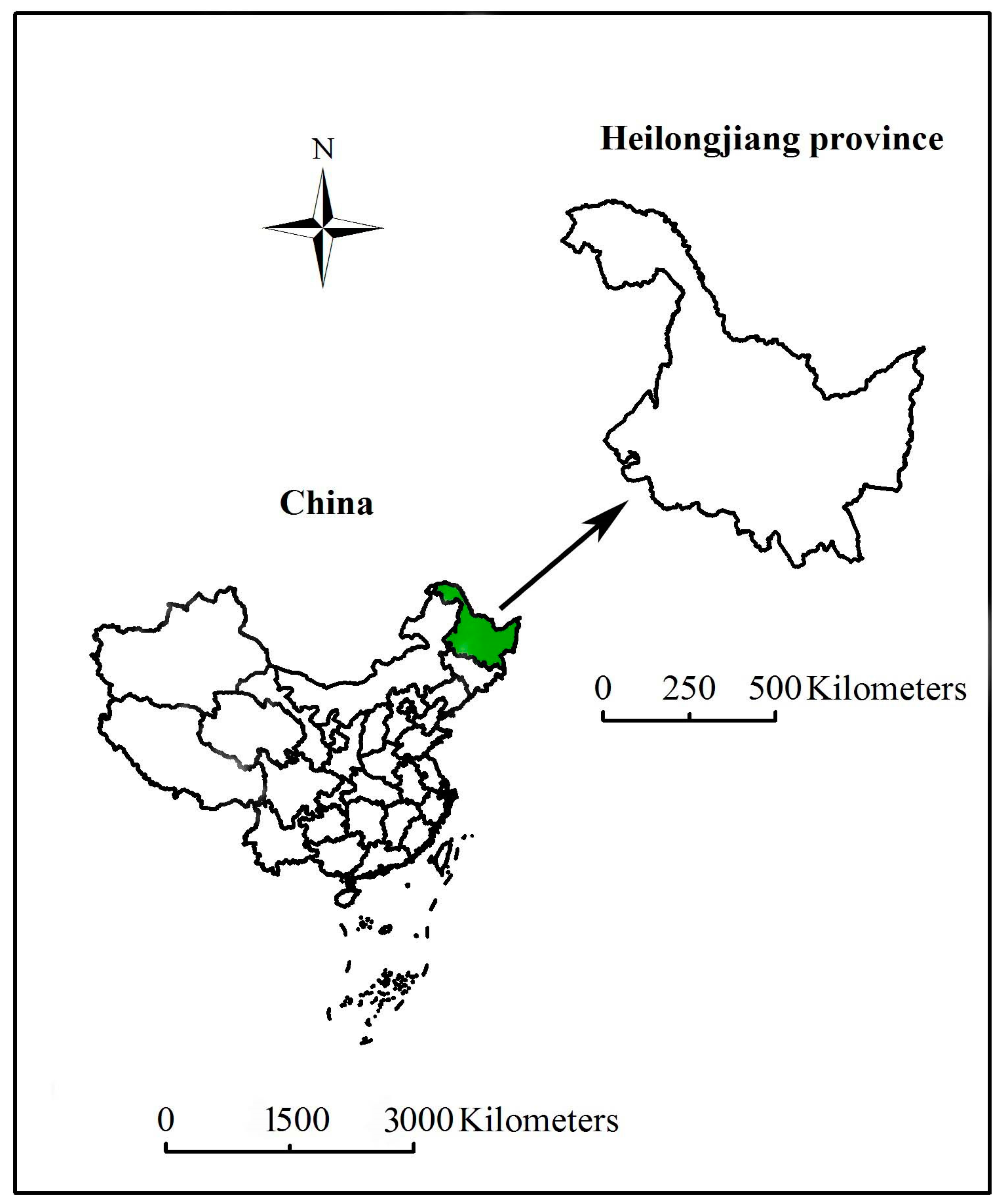
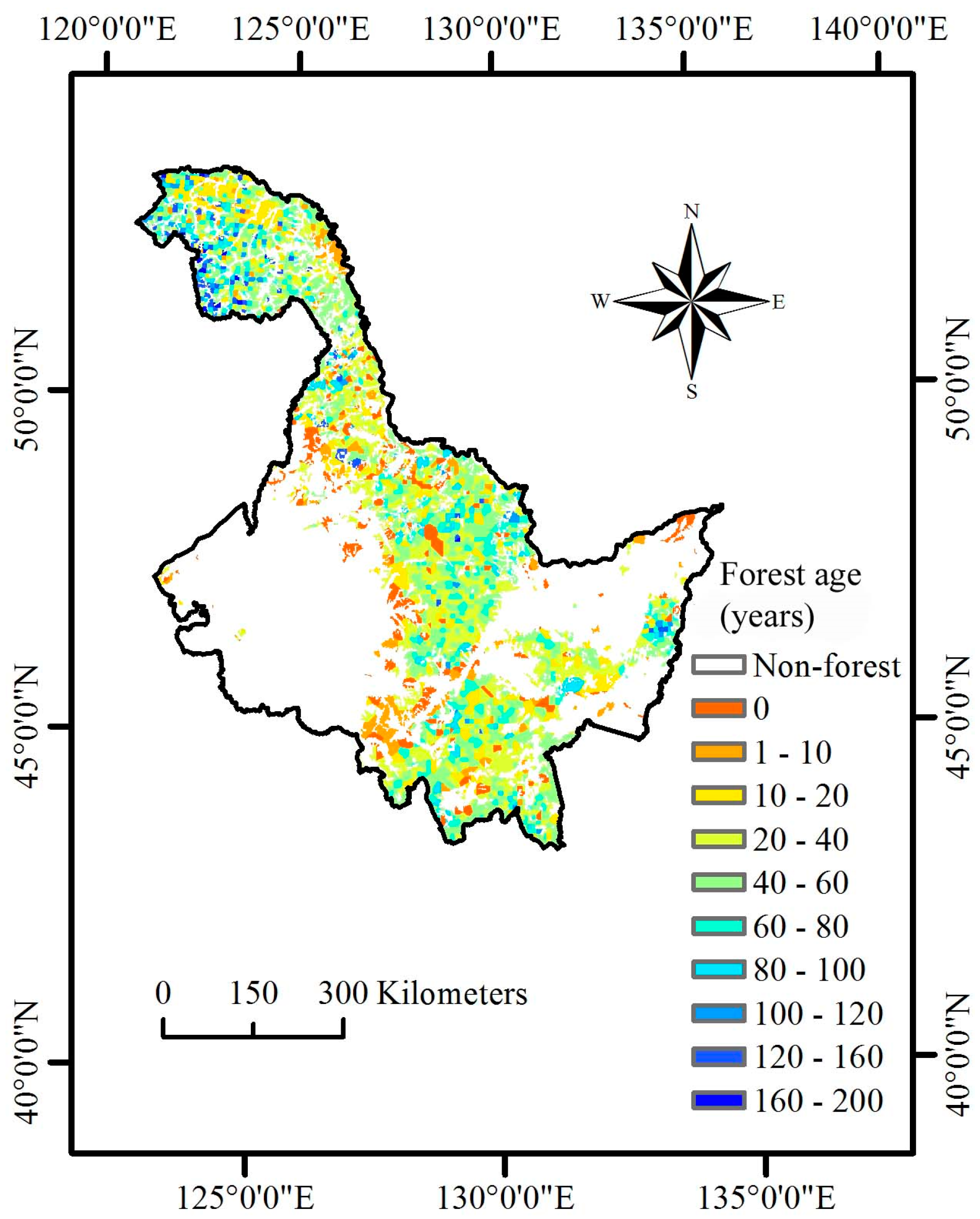
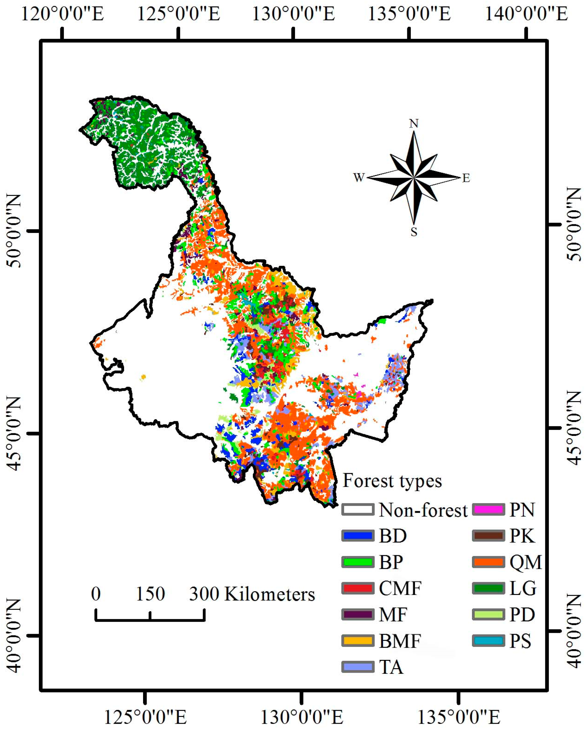
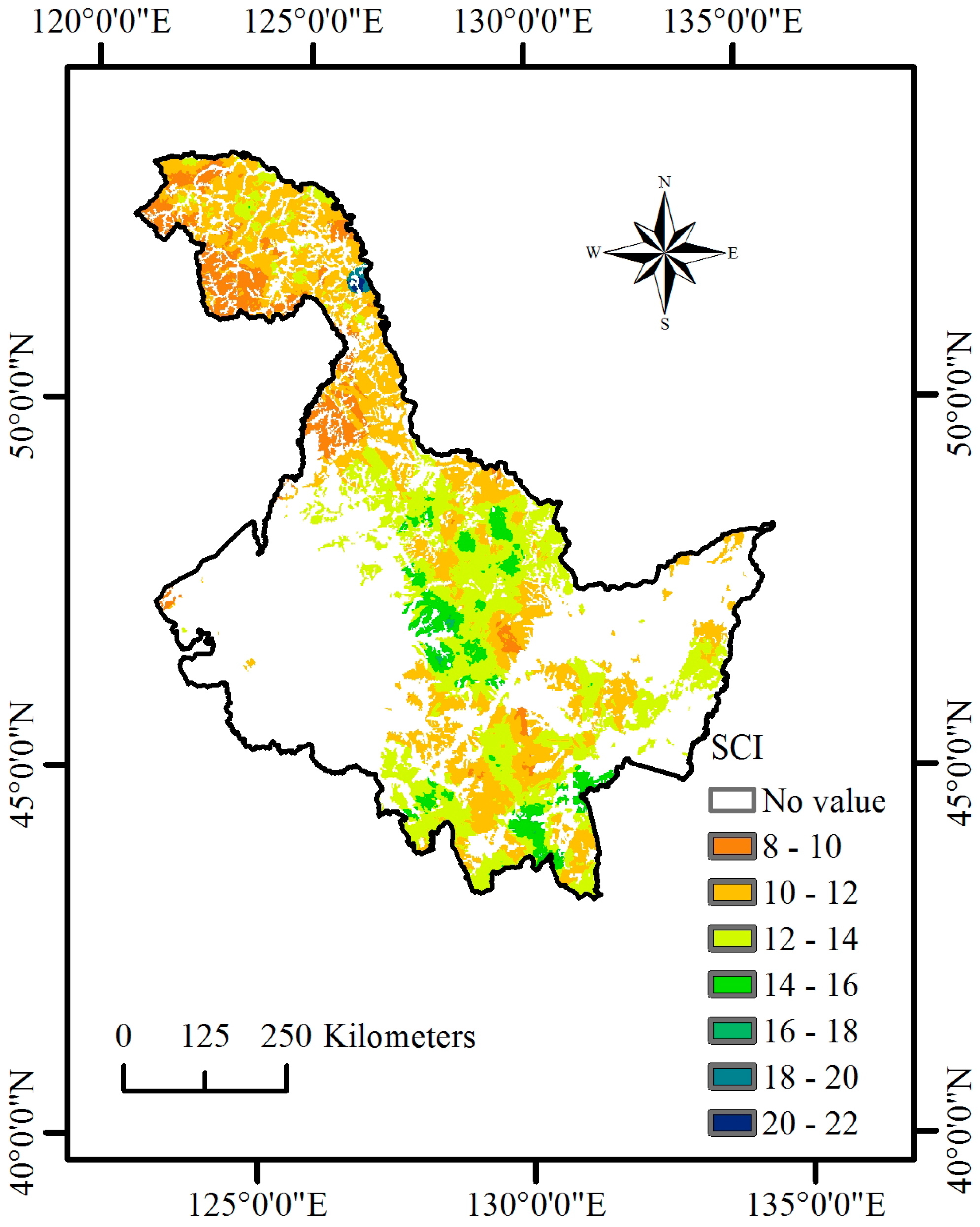
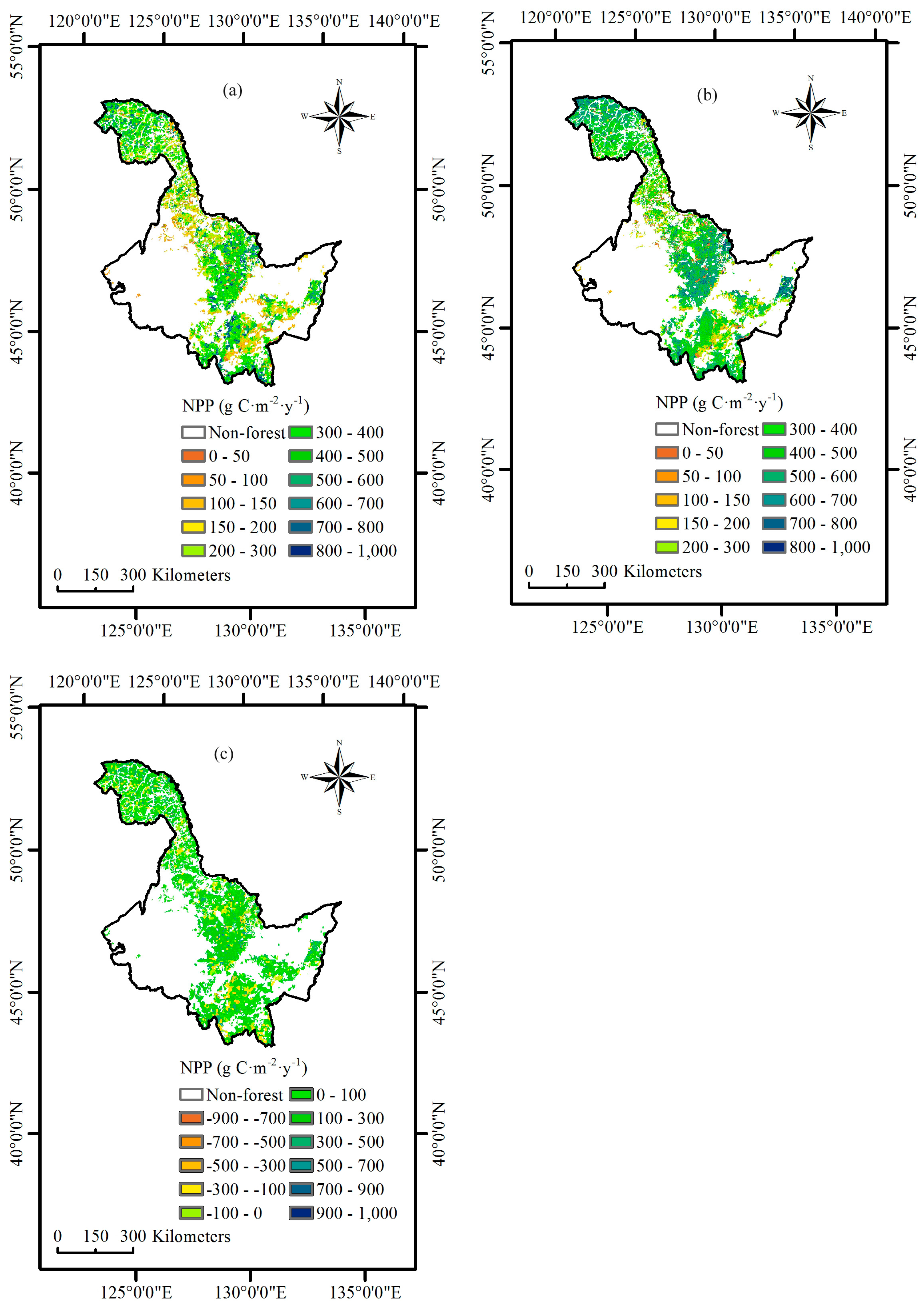
Until now, none of the existing regional C cycle modeling has incorporated systematic NPP-age relationships at various site class index (SCI) values in Heilongjiang Province, China. Heilongjiang Province (121°11′ E to 135°05′ E and 43°25′ N to 53°33′ N) is located in Northeast China (Figure 1). The province has a total forest area of over 20 million ha, which is about 45.8% of the total land area of the province, and the forest coverage rate is 45.7%. The total volume of living trees is 1.76 billion m3 and the average volume per hectare is 78.6 m3. In addition, the forest fire hazard in Heilongjiang Province is the highest of any area in China [27]. Therefore, the objectives of this study were to develop systematic NPP-age relationships at various SCI values for major forest types and groups in Heilongjiang Province, China, by combining data from forest inventories and stand yield tables, and to examine whether the new NPP-age relationships at various SCI values could estimate NPP through C cycle modeling.

2. Data Set

2.1. Forest Inventory Data and Yield Tables

The Forest Inventory data set was derived from the eighth national forest inventory data recorded from 2009 to 2014 in Heilongjiang Province [28]. The data set was measured periodically to provide statistics on stand age, H, DBH, and forest type.
Yield tables reflect the growth processes of forest stands with various stand structures and forest treatments. The yield tables of Heilongjiang Province, China were developed by the Forest Survey Scheme Designing Institute in 2010, and they provided information on the forest, such as forest type, mean age, DBH, H, stand density (S), volume (V) for different forest types and groups, and SCI. Based on this information, the standing live biomass can be calculated. A five-year age interval is used in the yield tables.

2.2. Input Data in the InTEC Model

The Integrated Terrestrial Ecosystem Carbon (InTEC) model is a process-based biogeochemical model driven by monthly climate data, vegetation parameters, and forest disturbance information. The model can estimate the effects of changing climate, atmospheric composition, disturbance, and forest recovery on the long-term C and N cycles in forest ecosystems.
To drive the InTEC model, a series of datasets were created in this study. All spatial data are listed in Table 1 and employed in the UTM projection WGS-84 coordinate system and interpolated to a one kilometer resolution.
The monthly mean temperature, relative humidity, and total precipitation for Heilongjiang in China from 1901 to 2010 were obtained from 0.5° global data set interpolated by the UK Climate Research Unit [29]. The dataset was produced by measurements taken at available stations of the National Meteorological Administration in China. Monthly solar irradiance data for the period prior to 1948 was produced by the Bristow-Campbell model [30] derived from the historical temperature, humidity, and precipitation data. For the period from 1948 to 2010, monthly solar irradiance data from the T62 Gaussian reanalysis data of the U.S. National Center for Atmospheric Research (NCAR) were used [31].
The annual atmospheric CO2 concentrations from 1958 to 2010 were taken from the dataset obtained at the Mauna Loa Observatory (20° N, 156° W) [32]. The pre-1958 CO2 concentrations were estimated based on the Canadian Global Coupled Model (CGCM2) [33].
Spatial nitrogen (N) deposition data in 1993 were obtained from a dataset that was simulated based on a chemical transport model (TM3). This dataset included the predicted value of N deposition in 1860, 1993, and 2050, and the spatial resolution was 5° in longitude and 3.75° in latitude. Spatial N deposition from 1901 to 2010 (except 1993) was calculated based on historical greenhouse gas emissions and the average N deposition data in 1993 [21].
A map of forest stand age in 2010 (Figure 2) was produced from the eighth national forest inventory data recorded from 2009 to 2014 in Heilongjiang Province [28]. Stand age for each pixel was estimated by interpolation (kriging) [34].
The forest type map of Heilongjiang at a one km resolution (Figure 3) was obtained from the Northeast Institute of Geography and Agroecology, Chinese Academy of Sciences, published in 2007 [35]. The scale of the map is 1:1,000,000.
The physical properties of the soil, including the field capacity of soil water, soil depth, wilting point, and the fractions of clay, silt, and sand, were included. Field capacity and wilting point were derived from the International Geosphere-Biosphere Programme, Global Gridded Surfaces of Selected Soil Characteristics [36]. Soil depth was derived from the global soil texture dataset from Oak Ridge National Laboratory Distributed Active Archive Center, Tennessee, U.S. [37]. The fractions of clay, silt, and sand were obtained from the Harmonized World Soil Database (HWSD) constructed by the Food and Agriculture Organization of the United Nations (FAO) and the International Institute for Applied Systems Analysis (IIASA) [38].
A maximum leaf area index (LAI) map was produced in 2003 by Deng et al. [39] using SPOT-VEGETATION data based on an algorithm that considers the bidirectional distribution reflectance function (BRDF). Detailed descriptions of the 2003 LAI map and data processing methods are reported elsewhere [39].
NPP in 2003 was selected as the reference year. Wang et al. [40] produced a NPP distribution map in 2003 using the BEPS model, and the reference year NPP data were used to calibrate the initial value of NPP in InTEC.
Because SCI was defined as the average height of a forest stand at a predetermined age, the national forest inventory data can offer both age and height information for producing SCI distribution maps in Heilongjiang Province (Figure 4). The minimum SCI is eight, the maximum is 22, and the average is 14. We assume that SCI is unchanged during the model simulation period.

3. Methods

3.1. SCI and NPP Calculation

SCI is defined as the mean tree height in a specific base stand age (20–50 years old) of a site. It can be calculated using the following two equations which were published in yield tables: Equation (1) is for Pinus koraiensis and Pinus sylvestris forests, and Equation (2) is used for other forest types and groups:
S C I = H   exp [ k ( 1 / t I 1 / t ) ]
S C I = H [ 1 exp ( k t I ) ] c [ 1 exp ( k t ) ] c
where H represents the mean tree height for a specific forest stand; tI is the base stand age; t is the current mean age of forest; and k and c are regression coefficients. The tI, k, and c values are listed in Table 2 and were published in yield tables.
We estimated the NPP of a forest over a year as the sum of four components. The first was change in biomass (∆Btree), including stems (∆Bs), branches (∆Bb), foliage (∆Bf), and roots (∆Br). The second component was mortality, which includes standing dead trees and downed dead wood (Mtree). The third component was tissue turnover (Ltree), including the turnover of foliage (Lf) and fine roots (Lfr) in soil. The last component was the NPP of the understory vegetation and moss (NPPund). Hence, NPP over a year could be calculated using the following equation [17]:
N P P = Δ B t r e e + M t r e e + L t r e e + N P P u n d

3.2. The First Component of NPP—Change in Biomass

The biomass of several forest components can be calculated using the stand information in yield tables and biomass equations. In the single-tree additive system of biomass equations for the main tree species in Heilongjiang Province, that was produced by Dong et al. [41,42], the biomass equations contained only DBH and were constructed based on allometric equations.
For three mixed forest type groups, a stand biomass equation produced by Dong et al. [42] was used to estimate the biomass of the main forest type groups in Heilongjiang Province. These biomass equations contained both tree basal area (G) and H.
Growth equations include the Logistic equation, Mitscherlich equation, Gompertz equation, Richards equation [43], and Korf equation [44]. In this study, we found Korf equation fitted the biomass data well for broadleaved mixed forests and coniferous and broadleaved mixed forests with an R2 larger than 0.997. Meanwhile, Richards equation produced better model fitting for the other forest types (R2 = 0.995–0.999). The Richards and Korf equations were computed by Equations (4) and (5), respectively. Hence, the change in biomass at age i (∆B(i)) could be calculated by the first-order derivative of the Equations (4) and (5).
B = A × ( 1 e b t ) c
B = A × e b t c
where B is biomass in t/hm2, including Bt, Bs, Bb, Bf, and Br; t is stand age in years; and a, b, and c are coefficients of tree growth equations that are listed in Appendix A Table A1 and Table A2.

3.3. The Second Component of NPP—Mortality

Mortality represents a substantial component of C cycling. The yield tables do not include information about standing dead trees and the downed dead wood. In this study we used the average mortality rate of biomass ( M R ¯ % ) for different age groups for nine forest types and three forest type groups in Heilongjiang Province that were published by Jia [45]. We used M R ¯ % instead of a mortality equation due to insufficient mortality information in the yield tables. Average mortality rates for the main forest types and groups of Heilongjiang Province are only a crude approximation of the actual mortality. We limited mortality to a constant value after a forest was considered mature. Past research had indicated that there was no relationship between mortality and SCI [46]. The average mortality rates for the 12 forest types and groups are listed in Table 3.

3.4. The Third Component of NPP—Tissue Turnover

We calculated the foliage turnover as the product of foliage biomass and a species-dependent turnover rate as [26]:
L f = B f × T f × C f
where Bf is the biomass of foliage and Tf is the foliage turnover rate that differs by forest types. For broadleaved forest (DBF), Tf was 1. Cf is the C content in foliage, (Cf = 0.5) [47].
Thornton et al. [48] found a relationship between the turnover of foliage and the turnover of fine roots, so Lfr could be calculated using the following equation:
L f r = L f × e
where e is the new fine root carbon to new leaf carbon allocation. Tf and e are obtained from White [49] and are listed in Table 4.

3.5. The Fourth Component of NPP—The NPP of the Understory

The NPP of understory vegetation could not be calculated from yield tables and biomass equations, so we selected some sample plots on Maoer mountain in Heilongjiang Province to fit the change in NPPund with age. Fifty plots for three forest type groups were selected based on stand age, from young to mature. The plot size was 20 m × 30 m, further divided into four smaller plots that were located in each of the four quadrants of the plot. The area of these small plots was 1 m × 1 m. The tissues of annual herbs, new twigs, new foliage, and all fine roots with a diameter smaller than 2 mm were collected from the small plots. We first measured the fresh weight of these tissues then samples were dried at 70 °C and weighed to the nearest 0.1 g. NPPund was calculated as the sum of the dry biomass of herbs, new twigs, new foliage components, and new fine roots. We used nonlinear regression (SPSS 2017) to estimate NPPund as a function of stand age as [17]:
N P P u n d = A × e k × a g e
where A and k are empirical coefficients. This equation was applied for all ages in the range from 10 to 60. For all other ages, the maximum value of the equation for the age <10 and the minimum value for the age >60 were assigned due to the lack of data. The estimates of coefficients are listed in Table 5.

3.6. NPP-Age Relationships

We used nonlinear regression (SPSS 2017) to estimate NPP as a function of stand age and SCI as Equation (9). The equation was obtained by [26] that could fit the change in NPP at different ages and SCI, for each forest type and group:
N P P ( a g e , S C I ) = a [ 1 + b S C I ( a g e c ) d 1 e ( a g e c ) ]
where a, b, c, and d are coefficients depending on site conditions.
The R2 and RMSE of the relationship between NPP and age and SCI were listed in Table 6, where the R2 and the RMSE illustrated that the developed method could fit NPP-relationships at various SCI values well.

4. Results

4.1. Results for NPP-Age Relationships

The increase in biomass reached a peak in 10 to 20 years for broadleaved forests and in 20 to 30 years for coniferous forests (Figure 5 and Appendix A Figure A1). Afterward, the biomass increase began to decrease and was almost unchanged after the forest reached maturity; meanwhile, the foliage and fine root turnover became the main components of NPP at older ages. The mortality varied greatly with stand age; it generally reached a maximum after maturity due to competition from neighboring trees. The mortality of broadleaved forests was higher than that of coniferous forests. For the three mixed forest type groups, the maximum biomass increase in coniferous mixed forests was the least, and the age at which biomass growth reached a peak was the oldest. Broadleaved mixed forests had the largest biomass increase, with the peak growth age occurring at approximately 17 years, while in coniferous mixed forests and coniferous and broadleaved mixed forests it was approximately 20 to 30 years.
Different SCI values had different biomass increase curves, and from Figure 5 we found the sites that were the most productive due to having the better site conditions, shown by having higher maximum biomass increases and faster rates of biomass growth. The maximum biomass increase at maximum-SCI was up to two to three times greater than the minimum-SCI observed. The other components of NPP at the better sites were also higher than in the lower site conditions.
We divided the 12 forest types and groups into three main forest type groups: broadleaved forest (BF) (including BP, BD, TA, QM, PD, PN, and BMF), coniferous forest (CF) (including PK, LG, PS, and CMF) and coniferous and broadleaved mixed forest (MF). We compared all of the NPP for different age classes (young, mature, and old stands) in two categories of SCI values for the 12 forest types and groups, as shown in Figure 6 and Appendix A Figure A2. The NPP-age relationships at various SCI values for different forest types and groups presented similar trends. NPP increased with stand age initially, reached a peak, then declined due to slower biomass increases, and finally stayed relatively stable as determined by foliage and fine-root turnover in short time periods. However, for different forest types and groups, the age classes at which NPP reached a maximum were different. For BF and MF, the NPP increased rapidly and reached a maximum when young; thereafter, NPP began to decline gradually when mature and old. For CF, the maximum NPP occurred when a mature stand generally, and the range of NPP decline was smaller than BF and remained at a value of approximately 70% of the maximum in old age. Within the same forest type, higher SCI values led to a higher NPP and the extent of variation was greater than in the less-productive sites, where the trend was similar to the biomass increase. In reality, the effects of stand break-up or species succession on NPP could be significant, but they were not included in our analysis due to lack of data for the seed regeneration of trees.

4.2. Results for Combined NPP-Age Relationships into the InTEC Model

The average NPP of CF, BF, and MF were 330 g C·m−2·y−1, 296 g C·m−2·y−1, and 305 g C·m−2·y−1, respectively (Figure 7). From Figure 8, we found that the age of the majority of CF were between 40 and 60 years old, which was approaching the mature stand stage of CF. At this age, CF had greater carbon fixation capability than the other two forest type groups. However, 60% BF were between 20 and 60 years old, and at this time the NPP of BF began to decline. The NPP of MF was almost the same as CF, due to MF was younger than the other two categories, and this was during the period of the highest carbon fixation.
For the purpose of analyzing the influence of different SCI on NPP, we calculated the average NPP from 2000 to 2010 using SCI values of 10–12, 12–14, and 14–16 for the three main forest type groups (Figure 9), because we found that the distribution of SCI were concentrated mainly between 10 and 16. The average NPP of all the three forest type groups presented a similar fluctuating trend at various values of SCI. The larger values of SCI led to a higher NPP. For CF, the variation of NPP along SCI was not significant. For BF, the increase in NPP along SCI was more obvious than CF, where there was a 24% increase from minimum to maximum SCI. MF had the largest NPP increase, with an average NPP increase of 46% from minimum to maximum SCI.
We first compared the InTEC results of NPP in 2010 against the NPP before the NPP-age relationships were modified by the new NPP-age relationships at various SCI values in InTEC (Figure 10). After this modification with the new NPP-age curves, the average value of NPP for Heilongjiang Province was 389 g C·m−2·y−1. Nearly the entire north region of Heilongjiang had an NPP value above 400 g C·m−2·y−1. From Figure 3, we could find the main forest type was Larix gmelinii forest (in green), covering 78% in the north region of Heilongjiang, which had a stronger carbon sequestration capability than other forest types. The average NPP of the middle and south regions of Heilongjiang was divided into two levels and showed an increasing trend from north to south, which agreed with the trend of SCI (Figure 4). Before modification, the average value of NPP for Heilongjiang Province was 389 g C·m−2·y−1, showing only a small difference in the provincial average. However, there was a significant difference in the spatial distribution of NPP. Before this modification with the new NPP-age curves, we observed an obvious overestimate of NPP in the north and south region of Heilongjiang compared with that after modification. This is because the original InTEC model included only one curve (SCI = 14), however, we could find that (Figure 4) the real SCI in the north and south region of Heilongjiang should be lower than 14. This showed that the NPP-age relationships with different site conditions had significant differences and the NPP-age relationships which developed in this study make the spatial distribution of NPP more reliable for carbon cycle modeling.
Using the national forest inventory data, the NPP of every plot could be estimated using the same method as with yield tables. We compared the NPP results to measurements derived by [50] using InTEC, before and after the SCI modification of the NPP-age relationship (Figure 11). The R2 value of the linear regression increased from 40% to 53%, and RMSE reduced from 77 to 69 g C·m−2·y−1 after modification of the NPP-age relationships in InTEC with those derived from this study. These results showed the suitability of the method and that the new NPP-age relationships could improve the accuracy of NPP estimation using InTEC.

4.3. Uncertainties

The model for total living biomass had the highest accuracy (Table 7), and the mean absolute percent errors (MAE%) of the total estimated total biomass ranged from 12% to 15%, with a mean of about 14%. Broadleaved forest had the lowest precision among the three type groups. Estimated foliage biomass precision was obviously lower than total biomass; the MAE% ranged from 10% to 43%, with a mean of about 22%. Due to the yield tables not including information about mortality, hence we estimated mortality with the average mortality rate of biomass. We used the mortality data which was reported by Jia to estimate the error of mortality in our study. The MAE% for mortality was nearly 57% (ranging from 43% to 67%). We could not collect the measured data about tissue turnover (foliage and fine roots), however, based on a similar study published by Chen [17], the error for foliage turnover could be as high as 70% and 33% for the fine-root turnover. Due to the varying complexity of understory for different forest type groups, the estimate for NPPund also contained a high level of error, with a mean of about 52% (ranging from 41% to 66%).
The calculated NPP in this study was validated using NPP database created by Yu based on field measurements, which has been widely used to validate forest NPP [40,50]. The MAE% of our estimation of stand NPP ranged from 46% to 73%, with a mean of about 59%. The error was lower in the early stages of development because total NPP was dominated by the growth of the biomass components that could be estimated with comparatively low error. As stands developed, however, NPP became increasingly dominated by the turnover of roots and litterfall, both of which had a high level of associated error.
In NPP-age relationships at various SCI values, other errors may arise from errors inherent in the yield tables, as the age and SCI in the yield tables were also affected by sample sizes, site locations, environmental variability, and stand density. The parameters of Tf and e could not be obtained for the study region of China, so we used values from White et al. [49], which also brought associated error that could not be ignored.

5. Discussion

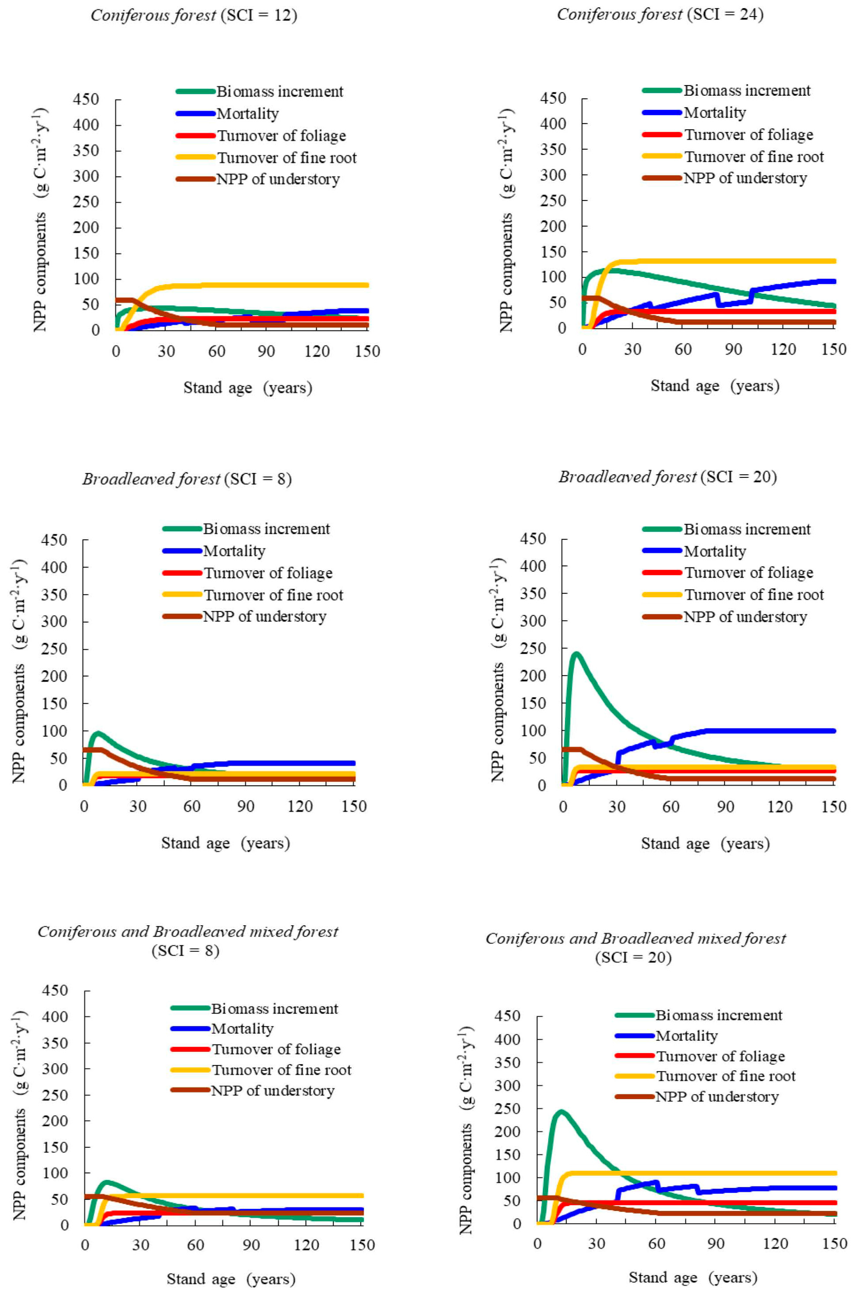
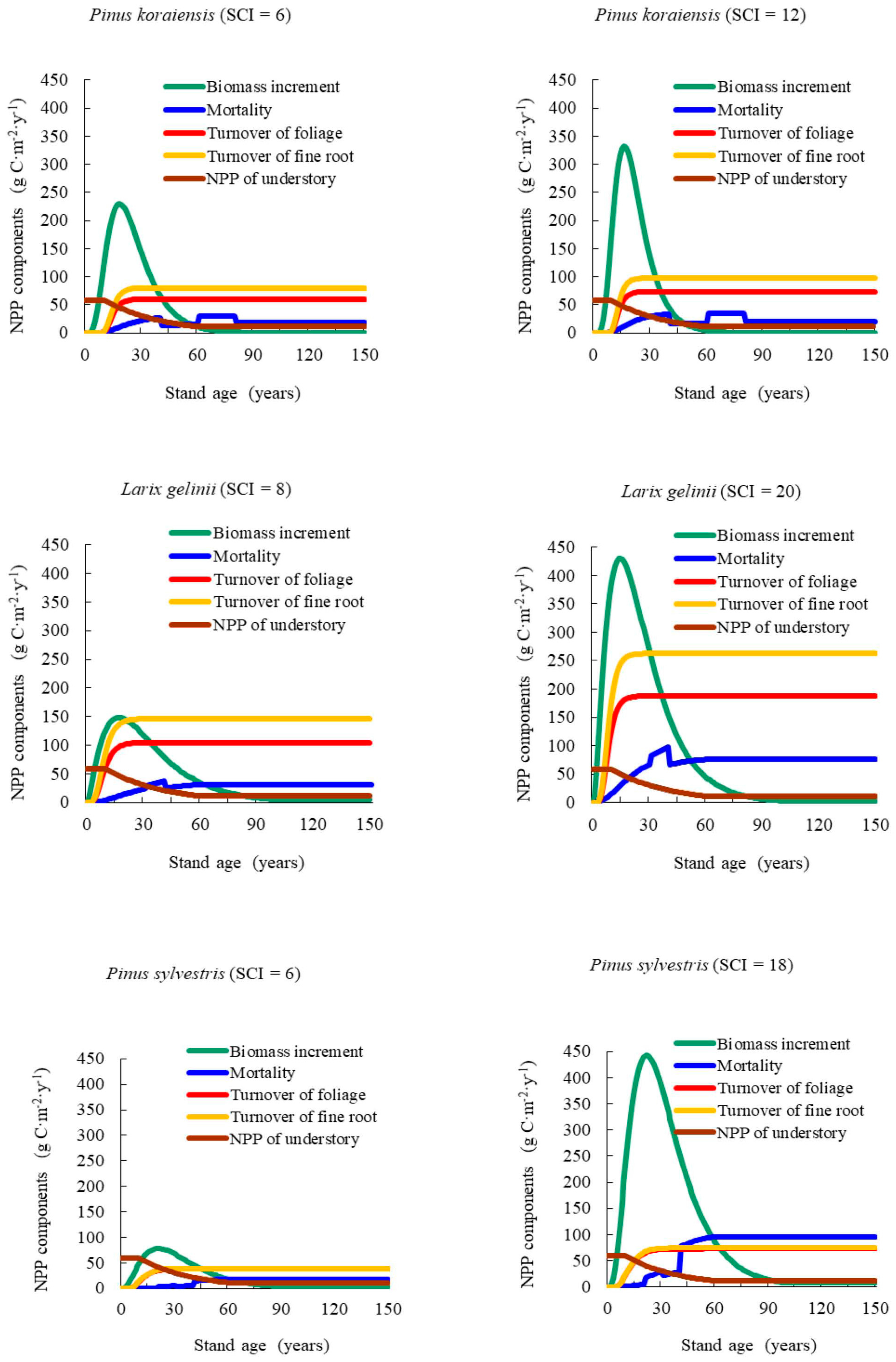
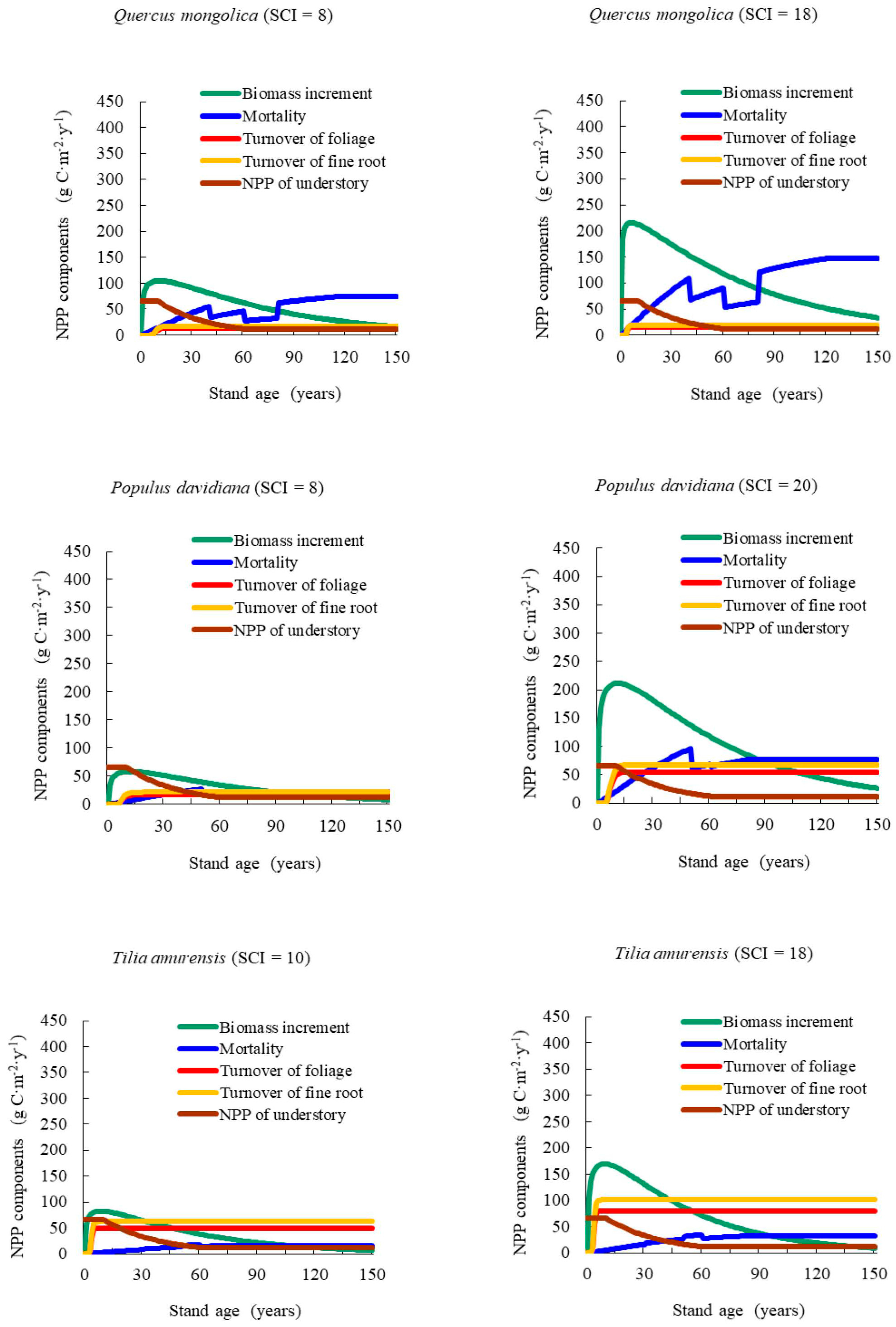
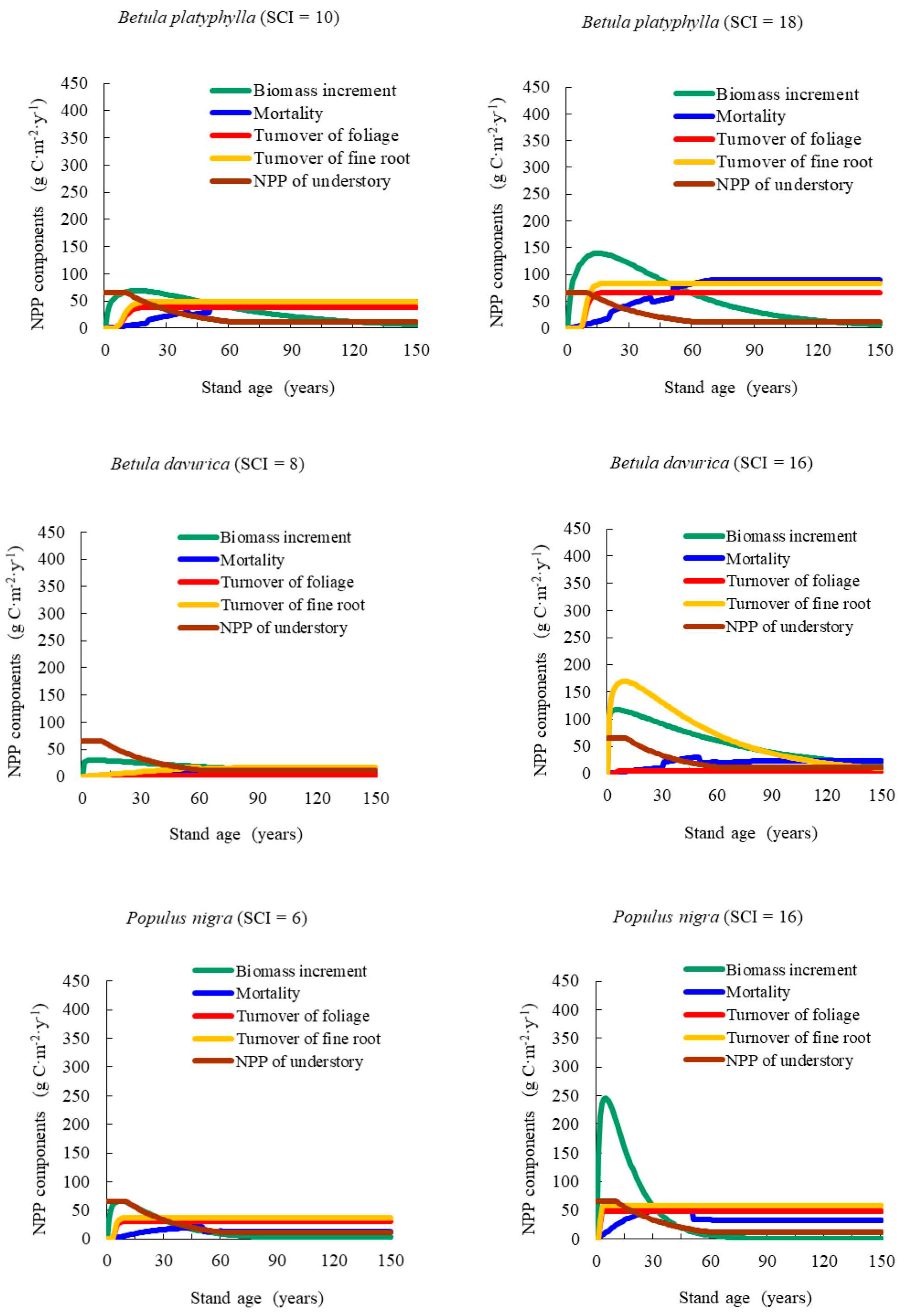
Our results showed that NPP varied with stand age and SCI, presenting a generally consistent trend of NPP-age relationships at various SCI values for different forest types and groups across the Heilongjiang Province, China. The NPP-age relationship curves at various SCI values were determined by components including the increase in total biomass, mortality, the fine root and foliage turnover rates, and the NPP of understory vegetation and moss. This method was similar in principle to that of Gower et al. [51] and Bernier et al. [52], who estimated stand-level NPP in a specific year using measured annual radial increased, biomass allometric equations, and measured foliage and root turnover rates. In the growth of young forests, NPP increasing rapidly with age was caused mainly by increases in biomass growth. Zha et al. [14] reported that aboveground NPP (ANPP) increased with age, stabilizing after 25 years. These results aligned well with those of our study. For old stand forests, where the products of photosynthesis were mainly consumed by foliage and fine root turnover, NPP began to decrease. Ryan et al. [13] reported that the range of NPP decreased by one half to one third from the peak growth period. Our results showed that it remained steady at 30% to 60% of the maximum NPP.
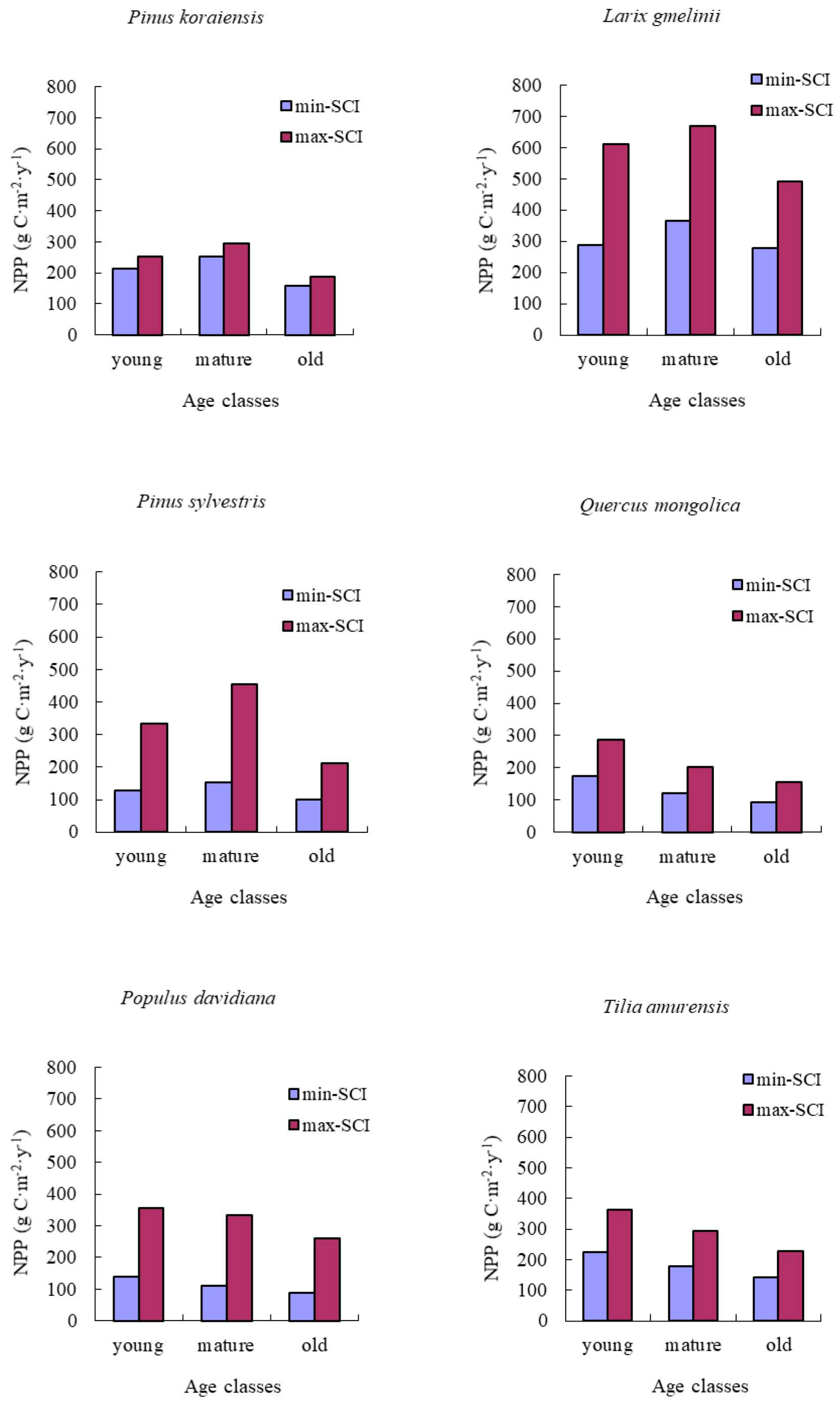
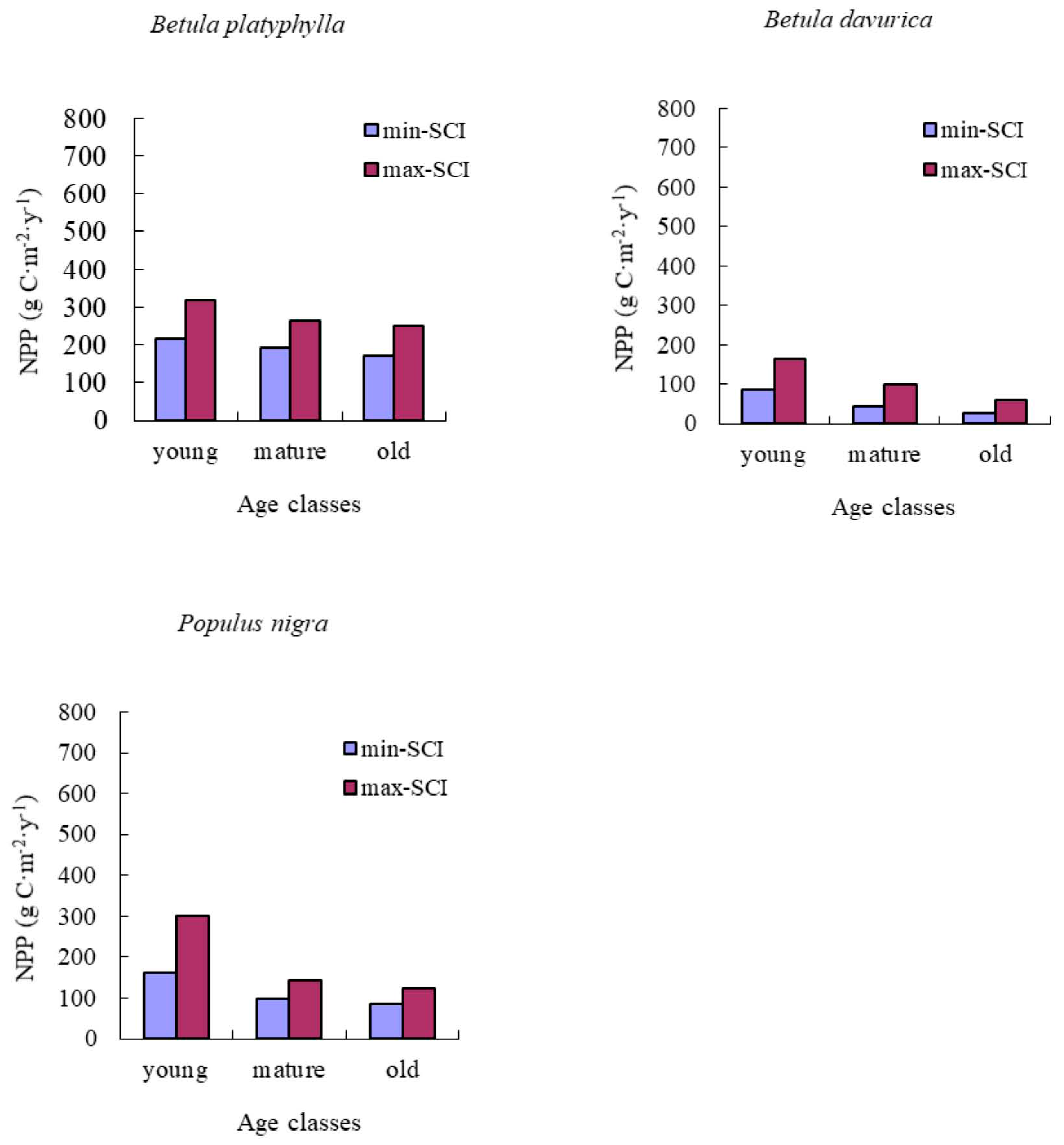
NPP-age relationships varied with site quality; higher productivity stands reached maximum NPP earlier than less productive stands. In addition, the decrease in NPP with age was also more dramatic for more productive sites. Our results were similar to those reported by Chen et al. [17].
We compared our NPP-age relationships with similar studies for China and the U.S. [24,26]. Our NPP-age curves were similar to the curves derived for China and U.S. forests except for DBF. Wang et al. [24] reported that the age at which the NPP reached peak value was always older, especially for DBF, which did not show a decline until the age of 120. However, our NPP-age relationships for DBF showed the decline of NPP at approximately 20 years of stand age. Three possible reasons included: first, there were only 37 samples from Heilongjiang Province in Wang’s study; second, Heilongjiang Province has fertile soil and earlier forest maturity than other regions; and lastly, the NPP-age relationships derived from BEPS modeling used in Wang et al. [24] may cause more error than that from yield tables.
Two studies had found old forests to be as productive as young forest stands [15,16]. In our study, the predicted NPP of old forests declined by an average value of 33% from its peak for all of forest types and groups studied. This may be caused by many other site factors, including climate, soil, and drainage. These factors caused the decline of biomass increase in old stands.
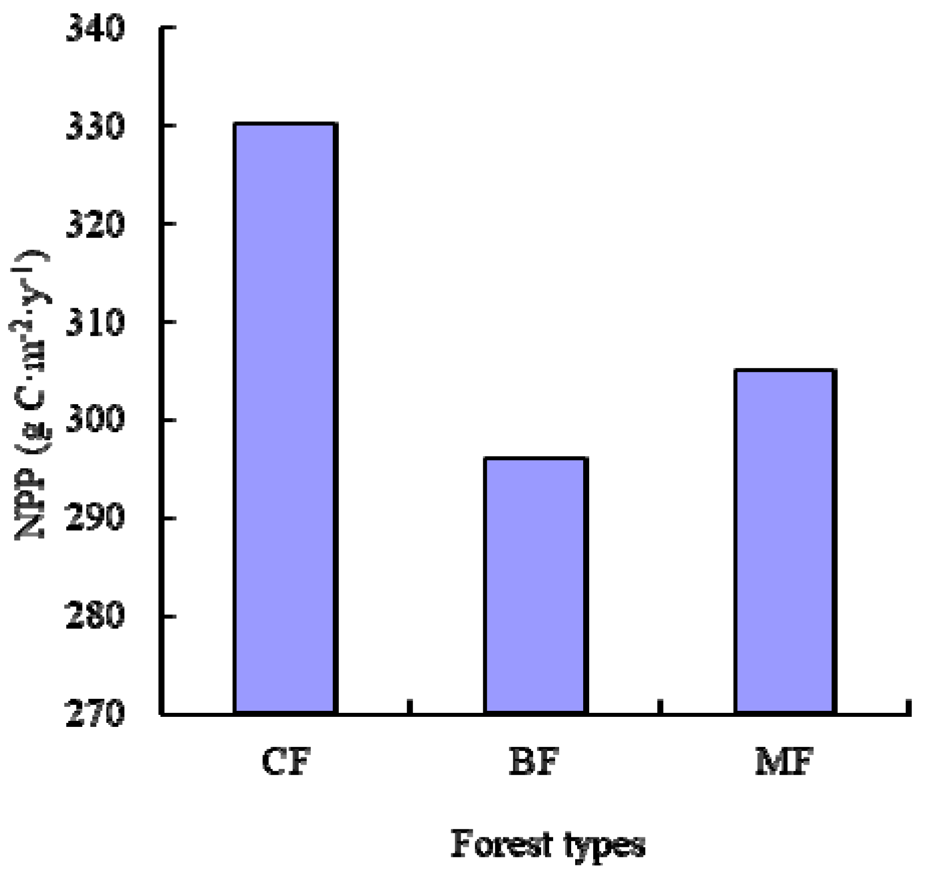
We implemented these NPP-age relationships into the InTEC model to estimate the NPP in Heilongjiang from 2000 to 2010. Our results showed that the average NPP of coniferous forest type groups was higher than that for the other two forest type groups. This aligned with the research of Mao et al. [53], which simulated NPP based on MODIS and AVHRR NDVI data sets. Our results also indicated the younger stands and higher SCI values may lead to a higher NPP, which agrees with the findings of Chen et al. [17]. However, the average NPP of the three main forest type groups was slightly lower than found in the research of Mao et al. [53]. MODIS NPP had been proven to oversimulate because the product was strongly driven by climate data [54].

6. Conclusions

In this study, we developed a specific method for estimating the relationships between NPP and age, at different SCI values for 12 forest types and groups, based on data from yield tables, biomass equations, and forest inventories. We derived the stand-level NPP through quantifying the four components: total biomass annual increment, tree mortality, turnover of foliage and fine roots, and the NPP of understory vegetation and moss.
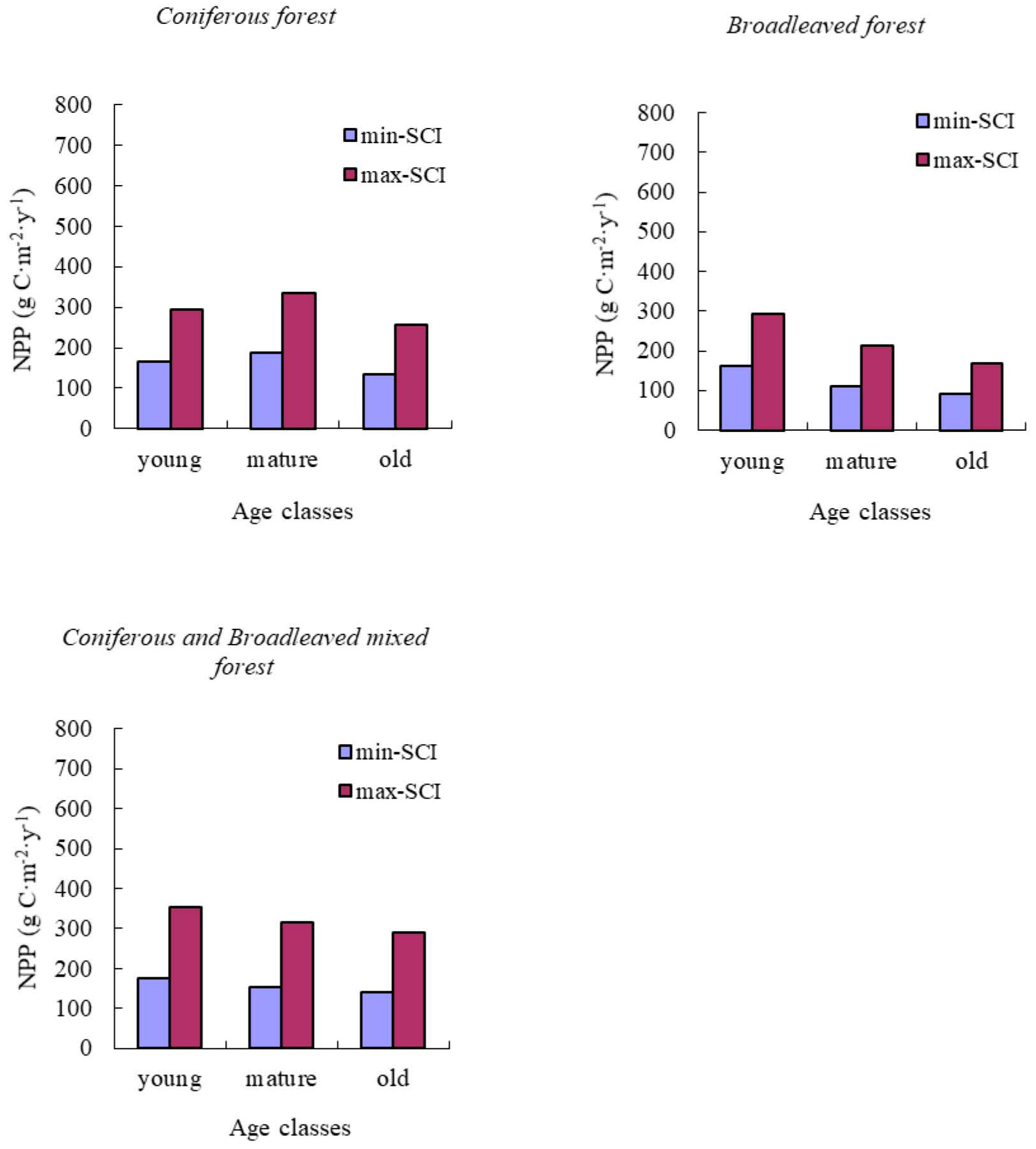
Two similarities in the temporal patterns of the NPP-age relationships at various SCI values occurred between various forest types and groups: first, NPP increased rapidly during early stages of stand growth, reached a peak when young or mature, and then declined after maturity; secondly, high productivity sites had higher maximum NPP than poor productivity sites.
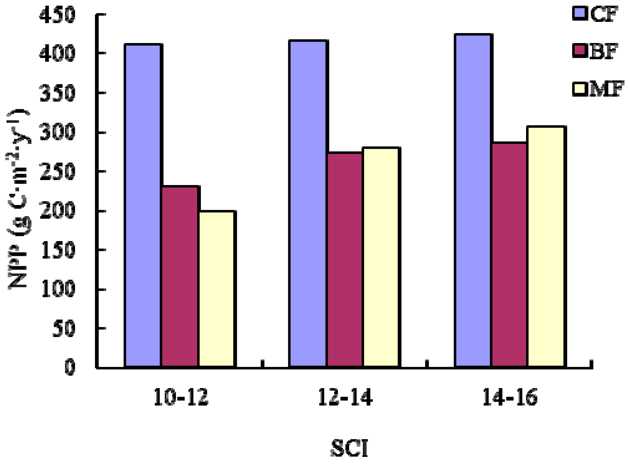
We implemented these NPP-age relationships at various SCI values into the InTEC model to estimate the NPP for three major forest biomes: coniferous forest, broadleaved forest, and mixed forest in Heilongjiang Province, China, from 2001 to 2010. During this period, the average NPP of coniferous forest was larger than broadleaved forest and mixed forest due to a greater carbon fixation capability and being productive at a mature age.
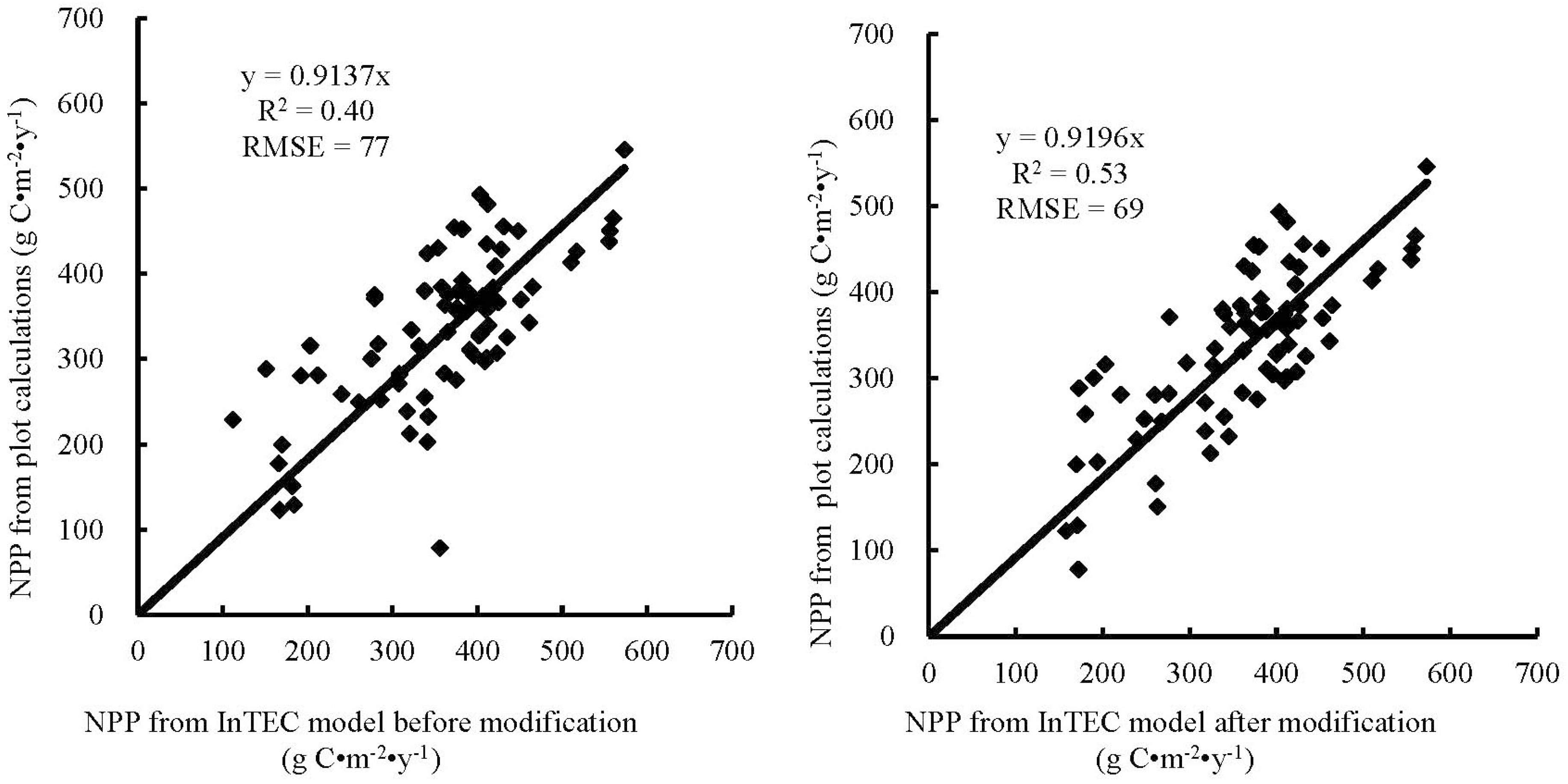
In this study, we also compared the results from InTEC modeling after modification with the new NPP-age relationships at various SCI values derived from this study. The model results showed that the new NPP-age relationships could better fit the NPP changes with age and SCI variation than the old ones used in the model.
However, there were still some weaknesses in our study: First, because mortality information was not included in the yield tables, we used the average mortality rate of biomass as the first order approximation; and second, the parameters of foliage and fine root turnover rates were obtained from White et al. [49] for North American forests, because of the lack of local measurements for these parameters. Our future studies could be directed toward acquiring this information in our region.
Although large uncertainties still exist in the development of these NPP-age relationships, this was nevertheless the first study in China to develop localized NPP-age relationships at various SCI values. These relationships have many potential uses for the analysis of forest management because they provide a new, independent, and comprehensive source of information on forest growth. This study should have implications for other forest regions of the world where SCI varies considerably.

Acknowledgments

Research grants from the National Natural Science Foundation of China (31470640, 31500518, 31500519, and 31300420), and the Fundamental Research Funds for the Central Universities (2572016AA30) supported this research. Models in support of this article were from the research collaboration with Jingming Chen at the University of Toronto; please contact mingzelee@163.com for details.

Author Contributions

Wenyi Fan, Jingming Chen and Mingze Li conceived and designed the experiments; Bin Wang performed the experiments; Bin Wang analyzed the data; Yu Ying contributed reagents/materials/analysis tools; Bin Wang and Mingze Li wrote the paper.

Conflicts of Interest

The authors declare no conflict of interest.

Appendix A

Figure A1. Variations of NPP components with age at minimum and maximum SCI for nine pure forest types.
Forests 09 00005 g0a1aForests 09 00005 g0a1bForests 09 00005 g0a1c
Figure A2. NPP for different age classes (young, mature, and old stands) in two categories of SCI values for the nine pure forest types.
Forests 09 00005 g0a2aForests 09 00005 g0a2b
Table A1. The Regression Coefficients for Equation (6) for nine pure forest types.
Forest TypeSCIAbcR2RMSENO.
Betula platyphyllaSCI = 105236.440.021.3899.9912.3613
SCI = 126201.100.021.4099.9916.8313
SCI = 147222.930.021.4399.9916.2413
SCI = 168366.930.021.4199.9916.8913
SCI = 188900.000.031.4999.9736.3413
Tilia amurensisSCI = 105682.840.021.1899.9625.2815
SCI = 126950.750.021.1799.9538.3315
SCI = 148238.550.021.1799.9641.4015
SCI = 169410.550.021.2199.9740.5715
SCI = 1810,702.490.021.2299.9748.4215
Betula davuricaSCI = 82999.990.011.0799.8121.7413
SCI = 104200.000.011.1099.7836.5213
SCI = 125699.990.011.0999.7948.8913
SCI = 147499.970.021.1099.7966.7813
SCI = 169499.950.021.0799.8571.8813
Pinus koraiensisSCI = 66035.830.095.2099.9253.3021
SCI = 86398.170.115.8999.9450.0621
SCI = 106687.730.116.3399.9358.3421
SCI = 126957.790.126.5599.8878.0621
Larix gmeliniiSCI = 86287.620.052.2899.9628.0617
SCI = 107905.530.052.3399.9638.4817
SCI = 129504.500.052.3099.9646.8017
SCI = 1410,808.280.062.3999.9746.9817
SCI = 1612,222.370.062.3799.9568.2717
SCI = 1813,096.630.062.5199.9753.0617
SCI = 2014,095.760.072.5699.9768.4917
Populus davidianaSCI = 84999.990.021.2299.7949.6815
SCI = 106799.990.021.2099.8457.3715
SCI = 128999.980.021.1799.8961.3415
SCI = 1410,599.970.021.2099.8394.8215
SCI = 1612,999.980.021.1899.8798.0215
SCI = 1815,099.990.021.2099.86119.7415
SCI = 2017,299.980.021.2099.83155.3515
Populus nigraSCI = 62300.000.051.3499.9411.0013
SCI = 82700.000.071.5599.8624.8513
SCI = 103500.000.061.4799.8927.7513
SCI = 123900.000.081.5699.8637.1713
SCI = 144700.000.071.4199.9622.5313
SCI = 165300.000.071.3699.9819.6413
Quercus mongolicaSCI = 89300.000.021.1899.52147.1519
SCI = 1011,300.000.021.1699.61157.8519
SCI = 1212,999.990.021.1399.71158.4819
SCI = 1415,699.990.011.0899.78155.5619
SCI = 1616,999.930.011.0999.76181.0219
SCI = 1818,599.980.011.0999.77197.6119
Pinus sylvestrisSCI = 63143.280.063.1699.9811.9021
SCI = 84861.320.063.3299.9721.6021
SCI = 106792.030.063.4299.9729.0621
SCI = 128998.500.063.5099.9838.0221
SCI = 1411,622.270.063.4199.9752.1921
SCI = 1613,999.990.063.6099.9859.1021
SCI = 1816,500.000.063.8199.9693.9821
Table A2. The Regression Coefficients for Equations (6) and (7) in three main forest type groups.
Forest Type GroupSCIAbcR2RMSENO.
Coniferous forestSCI = 128499.970.011.1999.9822.0029
SCI = 149399.970.011.2299.9638.2329
SCI = 1610,999.990.011.2099.9740.8929
SCI = 1812,999.990.011.1699.9831.2429
SCI = 2013,999.990.011.1899.9748.2829
SCI = 2215,999.880.011.1499.9936.8629
SCI = 2416,999.960.011.1599.9854.0429
Broadleaved forestSCI = 89800.007.900.4899.7860.8417
SCI = 1012,000.008.080.4999.8463.7617
SCI = 1215,500.007.770.4799.9252.6117
SCI = 1416,500.008.100.5099.9264.6717
SCI = 1619,000.008.000.4999.9461.8617
SCI = 1821,998.887.740.4899.9753.2317
SCI = 2023,999.997.740.4899.9755.1717
Mixed forestSCI = 88000.0012.160.6399.6970.5623
SCI = 1010,000.0012.120.6399.7973.1423
SCI = 1211,500.0012.580.6599.8281.0823
SCI = 1413,900.0011.700.6399.9070.7723
SCI = 1615,000.0012.370.6699.8985.6023
SCI = 1816,000.0013.090.7099.87103.8923
SCI = 2017,000.0013.780.7399.85122.8323

References

  1. Field, C.B.; Behrenfeld, M.J.; Randerson, J.T.; Falkowski, P. Primary production of the biosphere: Integrating terrestrial and oceanic components. Science 1996, 281, 237–240. [Google Scholar] [CrossRef]
  2. Pan, Y.D.; Richard, B.; Hom, J.; McCullough, K. Separating effects of changes in atmospheric composition, climate and land-use on carbon sequestration of U.S. For. Ecol. Manag. 2009, 259, 151–164. [Google Scholar] [CrossRef]
  3. Wang, S.Q.; Chen, J.M.; Ju, W.M.; Feng, X.F.; Chen, M.Z.; Chen, P.; Yu, G. Carbon sinks and sources in China’s forests during 1901–2001. J. Environ. Manag. 2007, 85, 524–537. [Google Scholar] [CrossRef] [PubMed]
  4. Birdsey, R.; Pregitzer, K.; Lucier, A. Forest carbon management in the United States. J. Environ. Qual. 2006, 35, 1461–1469. [Google Scholar] [CrossRef] [PubMed]
  5. Zhang, F.M.; Chen, J.M.; Pan, Y.; Birdsey, R.A.; Shen, S.H.; Ju, W.M.; He, L. Attributing carbon sinks in conterminous US forests to disturbance and non-disturbance factors from 1901 to 2010. J. Geogr. Res. 2012, 117, 1–18. [Google Scholar]
  6. Zhang, F.M.; Chen, J.M.; Pan, Y.D.; Birdsey, R.A.; Shen, S.H.; Ju, W.M.; Dugan, A.J. Impacts of inadequate historical disturbance data in the early twentieth century on modeling recent carbon dynamics (1951–2010) in conterminous U.S. forests. J. Geophys. Res. Biogeosci. 2015, 120, 549–569. [Google Scholar] [CrossRef]
  7. Williams, C.A.; Gu, H.; MacLean, R.; Masek, J.G.; Collatz, G.J. Disturbance and the carbon balance of US forests: A quantitative review of impacts from harvests, fires, insects, and droughts. Glob. Planet. Chang. 2016, 143, 66–80. [Google Scholar] [CrossRef]
  8. Pregitzer, K.S.; Euskirchen, E.S. Carbon cycling and storage in world forests: Biome patterns related to forest age. Glob. Chang. Biol. 2004, 10, 2052–2077. [Google Scholar] [CrossRef]
  9. Kurz, W.A.; Apps, M.J. A 70-year retrospective analysis of carbon fluxes in the Canadian forest sector. Ecol. Appl. 1999, 9, 526–547. [Google Scholar] [CrossRef]
  10. Price, D.T.; Halliwell, D.H.; Apps, M.J.; Kurz, W.A.; Curry, S.R. Comprehensive assessment of carbon stocks and fluxes in a boreal forest management unit. Can. J. For. Res. 1997, 27, 2005–2016. [Google Scholar] [CrossRef]
  11. Pan, Y.D.; Chen, J.M.; Birdsey, R.A.; McCullough, K.; He, L.M.; Deng, F. Age structure and disturbance legacy of North American forests. Biogeosciences 2011, 8, 715–732. [Google Scholar] [CrossRef] [Green Version]
  12. Pearson, J.A.; Knight, D.H.; Fahey, T.J. Biomass and nutrient accumulation during stand development in Wyoming lodgepole pine forests. Ecology 1987, 68, 1966–1973. [Google Scholar] [CrossRef]
  13. Ryan, M.G.; Binkley, D.; Fownes, J.H. Age-related decline in forest productivity: Pattern and process. Adv. Ecol. Res. 1997, 27, 213–262. [Google Scholar]
  14. Zha, T.S.; Barr, A.G.; Bernier, P.Y.; Lavigne, M.B.; Trofymow, J.A.; Amiro, B.D.; Arain, M.A.; Bhatti, J.S.; Black, T.A.; Margolis, H.A.; et al. Gross and aboveground net primary production at Canadian forest carbon flux sites. Agric. For. Meteorol. 2013, 175, 54–64. [Google Scholar] [CrossRef]
  15. Luyssaert, S.; Schulze, E.D.; Börner, A.; Knohl, A.; Hessenmöller, D.; Law, B.E.; Ciais, P.; Grace, J. Old-growth forests as global carbon sinks. Nature 2008, 455, 213–215. [Google Scholar] [CrossRef] [PubMed]
  16. Gough, C.M.; Curtis, P.S.; Hardiman, B.S.; Scheuermann, C.M.B. Bond-Lamberty Disturbance, complexity, and succession of net ecosystem production in North America’s temperate deciduous forests. Ecosphere 2016, 7. [Google Scholar] [CrossRef]
  17. Chen, W.J.; Chen, J.M.; Price, D.T.; Cihlar, J. Effects of stand age on net primary productivity of boreal black spruce forests in Ontario, Canada. Can. J. For. Res. 2002, 32, 833–842. [Google Scholar] [CrossRef]
  18. Fang, J.Y.; Chen, A.P.; Peng, C.H. Changes in forest biomass carbon storage in China between 1949 and 1998. Science 2001, 292, 2320–2322. [Google Scholar] [CrossRef] [PubMed]
  19. Chen, W.J.; Chen, J.M.; Cihlar, J. An integrated terrestrial carbon-budget model based on changes in disturbance, climate, and atmospheric chemistry. Ecol. Model. 2000, 135, 55–79. [Google Scholar] [CrossRef]
  20. Chen, W.J.; Chen, J.M.; Liu, J.; Cihlar, J. Approaches for reducing uncertainties in regional forest carbon balance. Glob. Biogeochem. Cycles 2000, 14, 827–838. [Google Scholar] [CrossRef]
  21. Chen, J.M.; Ju, W.M.; Cihlar, J.; Price, D.; Liu, J.; Chen, W.J.; Pan, J.J.; Black, A.; Barr, A. Spatial distribution of carbon sources and sinks in Canada’s forests. Tellus Ser. B-Chem. Phys. Meteorol. 2003, 55, 622–641. [Google Scholar]
  22. Chen, J.M.; Chen, W.J.; Liu, J.; Cihlar, J.; Gray, S. Annual carbon balance of Canada’s forests during 1895–1996. Glob. Biogeochem. Cycles 2000, 14, 839–849. [Google Scholar] [CrossRef]
  23. Ju, W.M.; Chen, J.M.; Harvey, D.; Wang, S.Q. Future carbon balance of China’s forests under climate change and increasing CO2. J. Environ. Manag. 2007, 85, 538–562. [Google Scholar] [CrossRef] [PubMed]
  24. Wang, S.Q.; Zhou, L.; Chen, J.M.; Ju, W.M.; Feng, X.F.; Wu, W.X. Relationships between net primary productivity and stand age for several forest types and their influence on china's carbon balance. J. Environ. Manag. 2011, 92, 1651–1662. [Google Scholar] [CrossRef] [PubMed]
  25. Zaehle, S.; Sitch, S.; Prentice, I.C.; Liski, J.; Cramer, W.; Erhard, M.; Hickler, T.; Smith, B. The importance of age-related decline in forest NPP for modeling regional carbon balances. Ecol. Appl. 2006, 16, 1555–1574. [Google Scholar] [CrossRef]
  26. He, L.M.; Chen, J.M.; Pan, Y.D.; Birdsey, R.; Kattge, J. Relationships between net primary productivity and forest stand age in U.S. forests. Glob. Biogeochem. Cycles 2012, 26, 1–19. [Google Scholar] [CrossRef]
  27. Wei, S.J. Quantitative Evaluation Methods of Carbon Emissions from Forest Fires in Heilongjiang Province, China. Ph.D. Thesis, Northeast Forestry University, Harbin, China, 2013; p. 46. [Google Scholar]
  28. FRSOC, Forest Resources Statistics of China (2009–2014); Department of Forest Resources Management State Forestry Administration: Beijing, China, 2016.
  29. Climatic Research Unit. Available online: http://www.cru.uea.ac.uk/cru/data/ (accessed on 20 July 2017).
  30. Thornton, P.E.; Running, S.W. An improved algorithm for estimating incident daily solar radiation from measurements of temperature, humidity, and precipitation. Agric. For. Meteorol. 1999, 93, 211–228. [Google Scholar] [CrossRef]
  31. Earth System Research Laboratory. Available online: https://www.esrl.noaa.gov/ (accessed on 20 July 2017).
  32. Carbon Dioxide Information Analysis Center (CDIAC). Available online: http://cdiac.esd.ornl.gov/ftp/trends/co2/maunaloa.co2 (accessed on 20 July 2017).
  33. Flato, G.M.; Boer, G.J. Warming asymmetry in climate change simulations. Geophys. Res. Lett. 2001, 28, 195–198. [Google Scholar] [CrossRef]
  34. Goldberger, A.S. Best Linear Unbiased Prediction in the Generalized Linear Regression Model. J. Am. Stat. Assoc. 1962, 57, 369–375. [Google Scholar] [CrossRef]
  35. Zhang, X.S.; Sun, S.Z.; Yong, S.P.; Zuo, Z.D.; Wang, R.Q. Vegetation Map of the People’s Republic of China; Geography Press: Beijing, China, 2007. [Google Scholar]
  36. IGBP-DIS. Available online: http://daac.ornl.gov/cgi-bin/dsviewer.pl?ds_id=569 (accessed on 20 July 2017).
  37. ORNL. Available online: https://www.ornl.gov/ (accessed on 20 July 2017).
  38. IIASA. Available online: http://daac.ornl.gov/SOILS/guides/HWSD.html (accessed on 20 July 2017).
  39. Deng, F.; Chen, J.M.; Plummer, S.; Chen, M.Z.; Pisek, J. Algorithm for global leaf area index retrieval using satellite imagery. IEEE Trans. Geosci. Remote Sens. 2006, 44, 2219–2229. [Google Scholar] [CrossRef]
  40. Wang, B.; Li, M.; Fan, W.; Zhang, F.M. Quantitative simulation of C budgets in a forest in Heilongjiang province, China. iForest 2016, 10, 128–135. [Google Scholar] [CrossRef]
  41. Dong, L.H.; Zhang, L.J.; Li, F.R. A compatible system of biomass equations for three conifer species in Northeast, China. For. Ecol. Manag. 2014, 329, 306–317. [Google Scholar] [CrossRef]
  42. Dong, L.H.; Zhang, L.J.; Li, F.R. Developing additive systems of biomass equations for nine hardwood species hardwood species in Northeast China. Trees 2015, 29, 1149–1163. [Google Scholar] [CrossRef]
  43. Richards, F.J. A flexible growth function for empirical use. J. Exp. Bot. 1959, 10, 290–300. [Google Scholar] [CrossRef]
  44. Korf, V. Příspěvek k matematické formulaci vzrůstového zákona lesních porostů. Lesnická Práce 1939, 18, 339–379. [Google Scholar]
  45. Jia, W.W.; Li, F.R. Forest Biomass and Carbon Storage for Different Forest Types in Northeast, China; Heilongjiang Science and Technology Press: Harbin, China, 2014. [Google Scholar]
  46. Clutter, J.L.; Fortson, J.C.; Pienaar, L.V.; Brister, G.H.; Bailey, R.L. Timber Management: A Quantitative Approach; John Wiley & Sons: Hoboken, NJ, USA, 1983. [Google Scholar]
  47. Yu, Y.; Fan, W.Y.; Li, M.Z. Forest carbon rates at different scales in Northeast China forest area. Chin. J. Appl. Ecol. 2012, 23, 341–346. [Google Scholar]
  48. Thornton, P.E. Description of a Numerical Simulation Model for Predicting the Dynamics of Energy, Water, Carbon, and Nitrogen in a Terrestrial Ecosystem. Ph.D. Thesis, University of Montana, Missoula, MT, USA, 1998. [Google Scholar]
  49. White, M.A.; Thornton, P.E.; Running, S.W.; Nemani, R.R. Parameterization and sensitivity analysis of the BIOME– BGC terrestrial ecosystem model: Net primary production controls. Earth Interact 2000, 4, 1–85. [Google Scholar] [CrossRef]
  50. Yu, Y.; Fan, W.Y.; Yang, X.G. Estimation of Forest NPP in Xiaoxing’an Mountains in 1901–2008. Sci. Silvae Sin. 2015, 10, 16–23. [Google Scholar]
  51. Gower, S.T.; Vogel, J.G.; Norman, J.M.; Kucharik, C.J.; Steele, S.J.; Stow, T.K. Carbon distribution and aboveground net primary production in aspen, jack pine, and black spruce stands in Saskatchewan and Manitoba, Canada. J. Geophys. Res. Atmos. 1997, 102. [Google Scholar] [CrossRef]
  52. Bernier, P.Y.; Fournier, R.; Ung, C.H.; Robitaille, G.; Larocque, G.; Lavigne, M.B.; Boutin, R.; Raulier, F.; Paré, D.; Beaubien, J.; et al. Linking ecophysiology and forest productivity: An overview of the ECOLEAP project. For. Chron. 1999, 75, 417–421. [Google Scholar] [CrossRef]
  53. Mao, D.H.; Wang, C.M.; Han, J.X.; Ren, C.Y. Spatio-temporal pattern of net primary productivity and its driven factors in Northeast China in 1982–2010. Sci. Geogr. Sin. 2012, 32, 1106–1111. [Google Scholar]
  54. Neumann, M.; Zhao, M.S.; Kindermann, G.; Hasenauer, H. Comparing MODIS net primary production estimates with terrestrial national forest inventory data in Austria. Remote Sens. 2015, 7, 3878–3906. [Google Scholar] [CrossRef]
Figure 1. Map of the study area in Heilongjiang Province, China.
Forests 09 00005 g001
Figure 2. Spatial distribution of forest age in Heilongjiang Province, China.
Forests 09 00005 g002
Figure 3. Spatial distribution of forest cover type in Heilongjiang Province, China. The map included three mixed forest type groups: coniferous mixed forest (CMF), broadleaved mixed forest (BMF), and coniferous and broadleaved mixed forest (MF), and nine pure forest types: Pinus koraiensis forest (PK), Larix gmelinii forest (LG), Pinus sylvestris forest (PS), Betula platyphylla forest (BP), Betula davurica forest (BD), Tilia amurensis forest (TA), Quercus mongolica forest (QM), Populus davidiana forest (PD), and Populus nigra forest (PN).
Forests 09 00005 g003
Figure 4. Spatial distribution of site class index (SCI) values in Heilongjiang Province, China.
Forests 09 00005 g004
Figure 5. Variations of NPP components with age at minimum and maximum SCI for three forest type groups.
Forests 09 00005 g005
Figure 6. NPP for different age classes (young, mature, and old stands) in two categories of SCI values for the three forest type groups.
Forests 09 00005 g006
Figure 7. Average NPP for the three main forest type groups in Heilongjiang province, China, from 2001 to 2010.
Forests 09 00005 g007
Figure 8. Pixel percentage for each stand age group for the three main forest type groups in Heilongjiang Province, China in 2010.
Forests 09 00005 g008
Figure 9. Average NPP for each SCI value for the three main forest type groups in Heilongjiang province, China, from 2001 to 2010.
Forests 09 00005 g009
Figure 10. Comparison of NPP from the InTEC model before (a) and after (b) modification of NPP-age relationship at various SCI values. Panel (c) is the difference between panel (a,b).
Forests 09 00005 g010
Figure 11. Estimations of NPP from the InTEC model before and after modification and from plot calculations.
Forests 09 00005 g011
Table 1. Descriptions of input data used in the InTEC model.
Data SetDescriptionResolution
Climate dataMonthly mean temperature, relative humidity, total precipitation and solar irradiance during 1901–2010.1 km
CO2 concentrationsMeasured data between 1958 and 2010 and Canadian Global Coupled Model (CGCM2) before 1958 [34]1 km
Nitrogen depositionChemical transport model [22]1 km
Forest stand age mapDeveloped from forest inventory data in 20101 km
Forest type mapDeveloped from CAS In 20061 km
Soil dataWilt point and field capacity of soil water, soil depth, fraction of clay, silt, and sand1 km
Leaf area indexDeveloped from SPOT4 VEGETATION data in 20031 km
Reference NPPDeveloped from BEPS model in 20031 km
SCI mapDeveloped from forest inventory data in 20101 km
Table 2. Coefficient estimates for Equations (1) and (2) for nine forest types and three forest type groups. tI is the base stand age in years, and k and c are regression coefficients.
Forest Type and Group t I k c
Pinus koraiensis3021.468-
Larix gmelinii300.0230.837
Pinus sylvestris3017.454-
Quercus mongolica500.0120.579
Populus davidiana300.0320.805
Tilia amurensis500.0290.838
Betula platyphylla400.0090.663
Betula davurica400.0210.775
Populus nigra200.0410.620
Coniferous forest800.0040.625
Broadleaved forest400.0110.541
Mixed forest500.0070.579
Table 3. The average mortality rate in percent volume change for nine forest types and three forest type groups.
Forest Type and GroupAge Group M R ¯ % Forest Type and GroupAge Group M R ¯ %
Pinus koraiensisYoung0.51Betula platyphyllaYoung0.75
Middle aged0.25Middle aged1.19
Near mature0.50Near mature0.99
Mature0.30Mature1.29
Larix gmeliniiYoung0.71Betula davuricaYoung0.33
Middle aged0.70Middle aged0.64
Near mature0.83Near mature0.40
Mature0.57Mature0.35
Pinus sylvestrisYoung0.11Populus nigraYoung1.08
Middle aged0.33Middle aged1.06
Near mature0.24Near mature0.66
Mature0.64Mature0.62
Quercus mongolicaYoung1.45Coniferous forestYoung1.12
Middle aged0.88Middle aged0.84
Near mature0.52Near mature0.56
Mature0.98Mature0.78
Populus davidianaYoung1.08Broadleaved forestYoung0.54
Middle aged1.06Middle aged1.09
Near mature0.66Near mature0.95
Mature0.62Mature1.06
Tilia amurensisYoung0.35Mixed forestYoung0.72
Middle aged0.39Middle aged1.08
Near mature0.46Near mature0.86
Mature0.37Mature1.93
Table 4. New fine root carbon to new leaf carbon allocation values and foliage turnover rates for 12 forest types and groups.
Forest Type and GroupTfe
Pinus koraiensis0.26 ± 0.151.4 ± 1.5
Larix gmelinii11.4 ± 1.5
Pinus sylvestris0.383 ± 0.021.33 ± 0.79
Quercus mongolica11.2 ± 1.2
Populus davidiana11.2 ± 1.2
Tilia amurensis11.2 ± 1.2
Betula platyphylla11.26
Betula davurica11.26
Populus nigra11.2 ± 1.2
Coniferous forest0.26 ± 0.151.4 ± 1.5
Broadleaved forest11.2 ± 1.2
Mixed forest11.3 ± 0.1
Table 5. Coefficient estimates and goodness-of-fit statistics of the NPPund equations.
Forest Type and GroupAkR2RMSENO.
Coniferous forest82.3720.0330.6116.115
Broadleaved forest92.7290.0340.6512.325
Mixed forest65.8230.0170.4213.410
Table 6. The four regression coefficients for Equation (9) for the nine forest types and three forest type groups.
Forest Type and GroupabcdR2RMSENO.
Pinus koraiensis1000.70218.01062.002888.8239.5888
Larix gmelinii1001.114315.31761.205897.9128.06126
Pinus sylvestris34.88651.693411.92591.870398.6215.9154
Quercus mongolica41.0380.92821.27960.459997.2211.93120
Populus davidiana35.31850.710946.11290.069898.1511.19112
Tilia amurensis120.72720.234447.64970.028398.1911.6180
Betula platyphylla54.66610.670227.18830.481299.126.7670
Betula davurica23.14530.713234.6920.062198.115.970
Populus nigra132.92820.39699.65220.497499.456.5884
Coniferous forest91.89270.270530.18840.550698.367.26210
Broadleaved forest57.63120.630515.95280.459498.469.01147
Mixed forest74.58470.50228.50170.316199.187.35168
Table 7. The Mean absolute percent errors (MAE%) of NPP and several components for the three main forest type groups.
Forest Type GroupNPP and ComponentsMean Absolute Percent Errors (MAE%)No.
Coniferous forestTotal biomass14173
Foliage biomass14173
Mortality43345
NPPund4915
NPP7331
Broadleaved forestTotal biomass152522
Foliage biomass432522
Mortality67497
NPPund4125
NPP4693
Mixed forestTotal biomass12519
Foliage biomass10519
Mortality61276
NPPund6610
NPP5854

