A New Method for Characterizing Bark Microrelief Using 3D Vision Systems

Abstract

Bark microrelief (BM), or the spatial patterning of bark texture, is an important bark characteristic shown to significantly affect the ecophysiological functioning of forest ecosystems. BM influences bark micrometeorological conditions and stemflow generation which, in turn, impacts epiphytic vegetation and microbial community patterns, as well as insect foraging behavior. Thus, an objective method to quantify BM is important to understand and model hydro-biogeochemical processes in forest canopy ecosystems. The aim of this study was to develop a method for fast and automated imaging of bark surface morphology. Three-dimensional imaging methods using laser triangulation were used to describe BM. An automated system was developed and applied to calculate three new BM indices for samples collected from five trees representing species common throughout Poland (and Northern Europe): common oak, European ash, trembling aspen, Scots pine, and black alder. These new BM indices may be useful for characterizing and quantitatively relating BM to forest canopy ecophysiological functions.

1. Introduction

Bark is the outermost layer of stems, branches, and roots of trees; it has several functions important both for the individual tree and the whole forest ecosystem [1,2,3]. In forest trees, bark plays an important role as the living environment for numerous organisms and as an influence of ecosystem water balance through rainfall retention [4]. Different adaptation strategies result in a wide variety of bark chemical and physical properties, and these affect the environmental functions of bark [5]. Apart from bark thickness, which is important for fire resistance [6,7], many tree species have adapted their bark to contain chemicals for better protection against insects or fungal attacks [8,9]. As a result of this adaptation, the bark of some tree species contains volatile oils and is waterproof [10]. Tree bark is also used as a bio-identifier of metal accumulation from road traffic [11,12]. It plays an important role in the accumulation of dichlorodiphenyltrichloroethane (DDT) from agricultural regions [13].

In order to extrapolate the results of bark water storage capacity, Levia and Herwitz [14] classified the species into rough-barked and smooth-barked. Roughness scales are often based on the maximal contact angle between liquid and the bark surface [10]. Unfortunately, this type of measurement cannot be taken from standing trees.

One of the most important bark characteristics is bark microrelief (BM), which is defined as the configuration of the bark surface with respect to the spatial patterning of bark texture [15]. BM variability of individual trees and species affects the ecophysiological functioning of forest ecosystems. BM is one of the important canopy structure metrics [16], which significantly affects both bark water storage capacity [4,17,18] and the distribution of lichens [19] and bryophytes [20]; together, these both directly affect stemflow yield and chemistry [21]. Authors also focus on tree bark from a mechanical perspective using optical techniques (e.g., stereoscopic 3D vision system) [22]. BM may also play a significant role in selecting the microbial community structure and function in the bark portion of the phyllosphere [23]. An objective method of quantifying BM is important for understanding and modelling the hydrological processes observed in forest ecosystems [24,25]. Tree bark is a basic container which intercepts water; therefore, improved quantitative characterization of BM is crucial in understanding the influence of tree species and stand age on water interception. This is especially important to hydrological modelling in forested areas. The authors of [26] show that BM plays a critical role in ant ecology as a factor influencing their running speed. It is also important to note that bark disease drastically alters BM [27].

To date, different methods of BM measurement and quantification have been developed. BM can currently be measured using the LaserBarkTM device (University of Delaware, Newark, USA) [23], wavelet analysis [28] and the coefficient of the development of the interception surface of bark [4]. A method has been presented that involves recording the profile of bark height using a triangular grid mounted on the tree trunk [23]. The method allows registration of only a single profile of bark around the tree perimeter. The work that outlines this [28] discusses the method of bark profile analysis that uses wavelet analysis. Wavelet analysis quantifies variations in bark microrelief around the perimeter of the tree. This measure describes the spatial differences in bark microrelief and allows for a representation of trees that exhibit directional variability in bark microrelief. The paper presented by Ilek and Kucza [4] proposes using the coefficient of development of the interception surface of bark as the quotient of the actual bark surface area and the cylindrical model surface.

Video methods have been successfully used in tests of wood surfaces for the detection of visible defects. Wood defects in the form of knars, cracks, and moldy areas are detected by grayscale or color analysis [29,30,31]; also used are tomographic [32], thermographic [33], and pH [34] analysis of images. Most vision systems may be described as two-dimensional due to the imaging method, the information stored, and the information made available in the image. 3D vision systems that facilitate spatial image acquisition [35] are also used in carrying out tasks related to the detection of defects and the measuring of surface defects introduced throughout wood processing. Three-dimensional images contribute to the determination of the x, y, and z coordinates of each point corresponding to the tested surface; this makes it possible to extend the image analysis in a direction normal to the tested surface.

Three-dimensional imaging was used to record an image of the bark surface using the laser triangulation method. The measuring stand was designed and configured for imaging and for bark surface tests of the prepared samples.

The aim of the research was to implement the project and run a 3D vision system using laser triangulation for fast and automated imaging of bark surfaces. This system was used to describe the parameters of bark morphology. As part of the research tests, algorithms were developed to speed up the analysis of surface images and the measurement of selected bark surface parameters. Additionally, the aim of the study was to determine the possibility of quickly measuring bark parameters in the field, directly on growing trees, and without the need for the laborious task of sample collection.

2. Materials and Methods

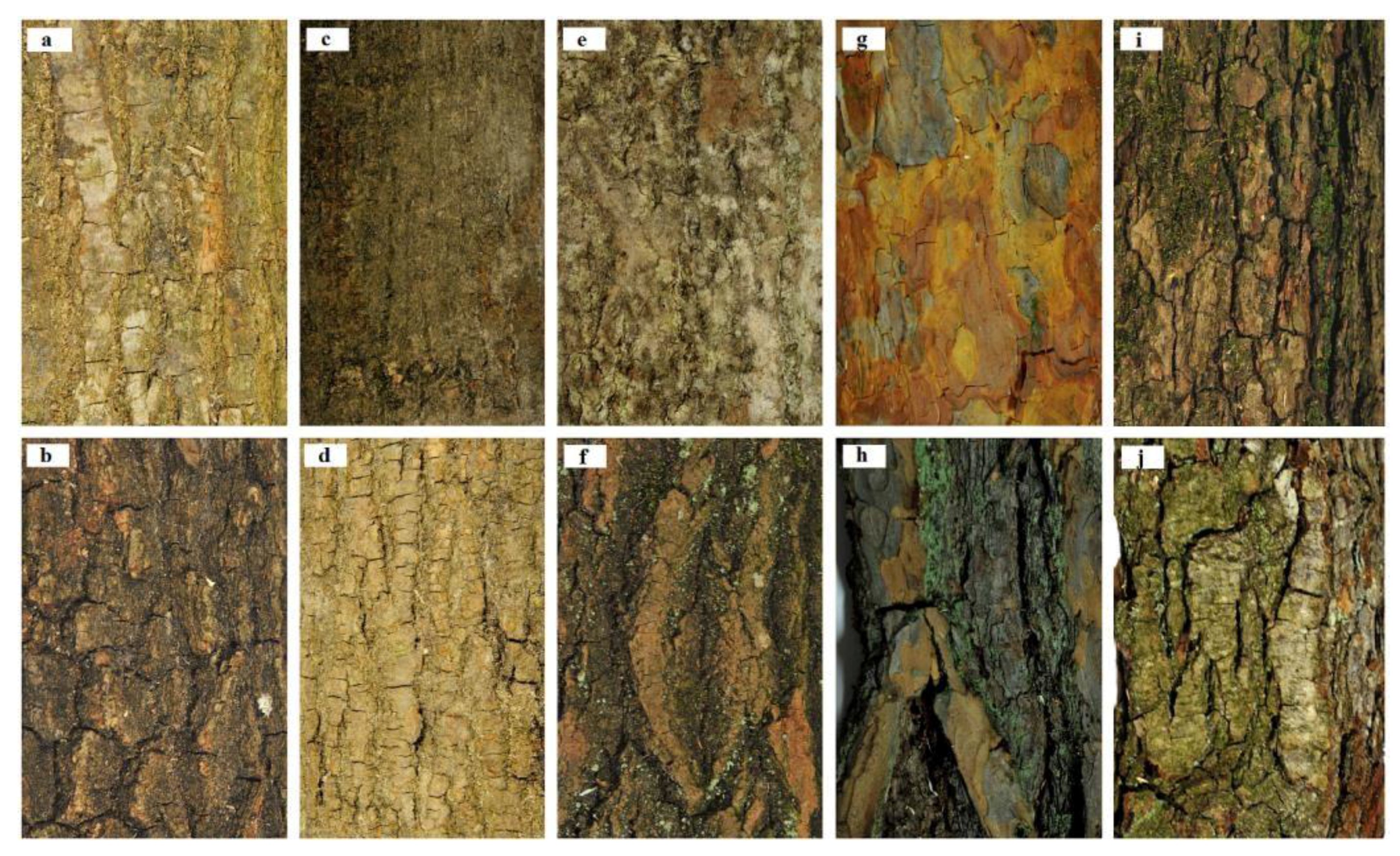
Bark samples were collected from 5 stands ~60 years in age from the mixed deciduous forest site in the Chełm Forest District of Eastern Poland In each stand one sample tree was felled for bark samples collection. A developed automated system was practically applied for the calculation of proposed indices for bark samples from 5 forest-forming tree species: common oak (Quercus robur L.), European ash (Fraxinus excelsior L.), trembling aspen (Populus tremula L.), Scots pine (Pinus sylvestris L.), and black alder (Alnus glutinosa Gaertn.) (Figure 1). To analyze intraspecific variability, BM characteristics for individual trees representing analyzed species were calculated from single bark samples collected from the lower and middle parts of the tree stem at the heights of 1.5 and 15 m above ground level, respectively.

The construction of a three-dimensional video system involves the selection of a hardware configuration (i.e., the type of camera), the type of optical system, and the laser illumination appropriate for the measurements.

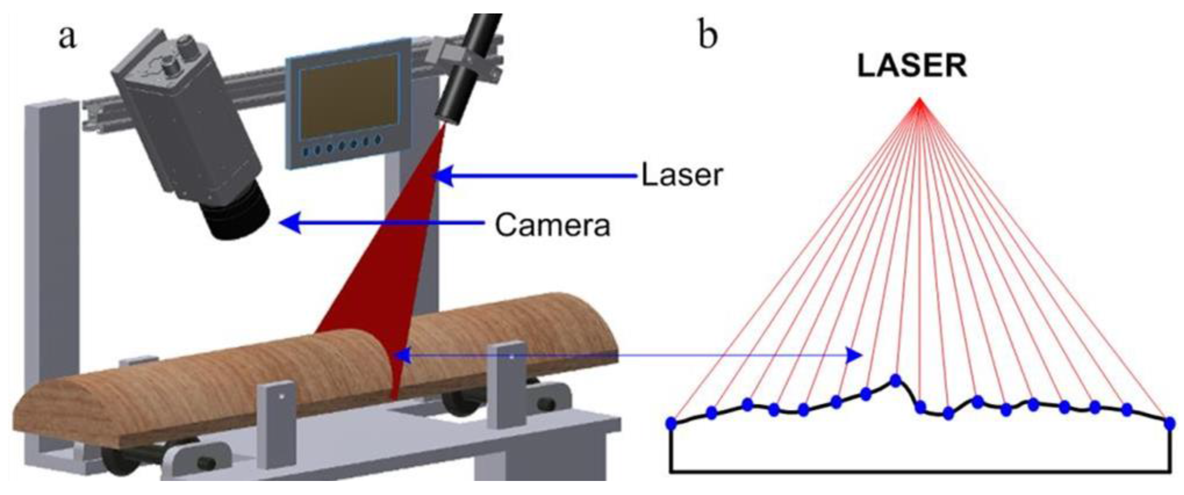
A 3D image is acquired from the analysis of 2D images recorded by a camera tracking the trace of a laser line displayed on the test surface (Figure 2a). Laser triangulation yields point distances along the laser line that can be converted into a height profile (Figure 2b). By moving the object relative to the video system, a set of profiles is defined which are then combined to form a three-dimensional image of the surface. An image consisting of 1000 elevation profiles, each comprised of 832 measurement points, was used for the study.

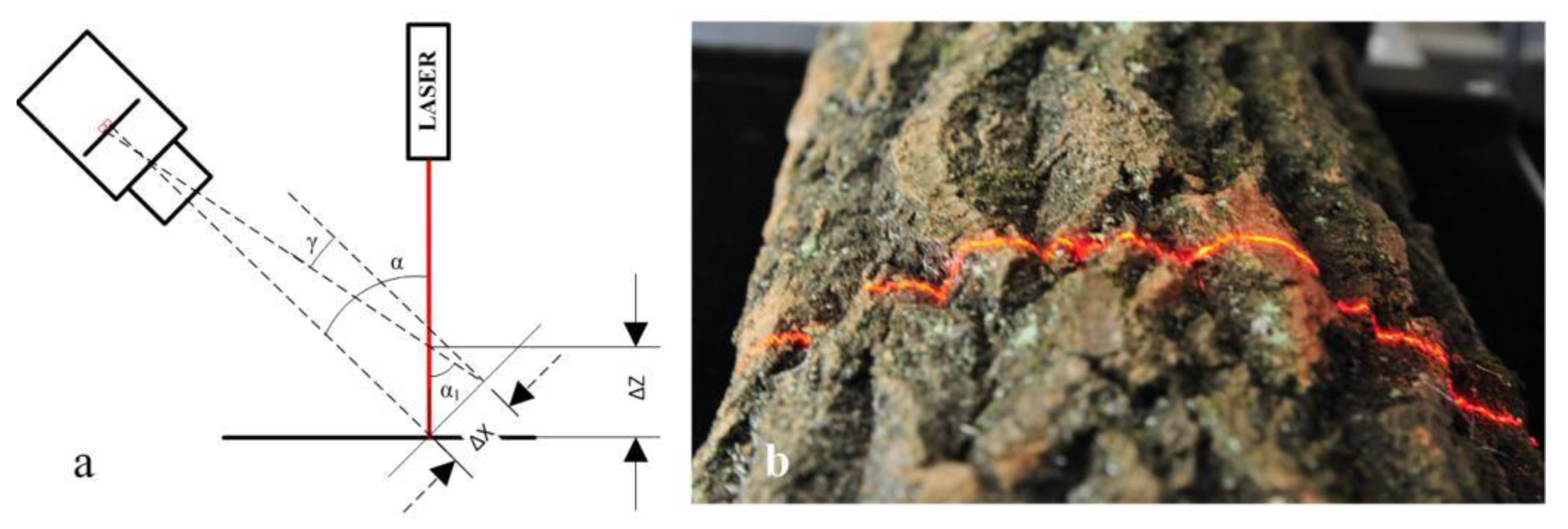
The geometry presented in Figure 3a, in which the video system sensor is set at a 90-α angle to the measuring table surface, was used for the measurement of bark parameters. The laser plane is perpendicular to the test surface and is set at an angle α relative to the optical axis of the camera (Figure 3a).

The bark profile determined from the analysis of the laser line image corresponds to the cross profile. This profile is observed by the vision system set at 90-α angle (Figure 3a). Consequently, it is necessary to convert the geometry of the section visible to the camera to be able to obtain the actual cross-section.

Each of the profiles marked on the examined surface is defined by a one-dimensional matrix of 832 × 1. It contains a set of values defining the height of measurement points marked along the laser line visible on the test surface (Figure 3b). Points defining the height profile are determined with a resolution dependent on the configuration used, the optical system used, and the resolution of the visual system matrix. Determining the resolution of the 3D vision system involves determining three components of resolution for each axis of the coordinate system. For the z-axis, it mainly consists of determining the minimal height change of the object described by the parameter ΔZ, at which there is an observed displacement of the laser image by exactly one pixel row on the camera matrix (Figure 3a). On the plane parallel to the matrix plane, a resolution of ΔX in the x-axis was determined on the basis of the field of view (FOV) dimensions and the matrix resolution given in pixels. ΔY resolution in the y-axis is defined as the distance between subsequent height profiles for the examined object.

ΔZ = ΔX/sin(α)

(1)

A matrix measuring 832 × 512 pixels was used for the tests. The field of view allows for viewing of a 166.4 mm wide object (i.e., FOV = 166.4 mm). The resolutions in the x and z-axes were defined as operating parameters of the video system.

∆X = 166.4 mm/832 pixels = 0.2 (mm/pixel)

(2)

When calculating resolution in the z-axis of the measurement position, it was assumed that the angle α was equal to α1. In fact, this angle α1 is equal to α − γ. Using this simplification, the resolution in the z-axis of the measurement position is determined by taking the angle α to be equal to 45° (Figure 3a).

ΔZ = ΔX/sin(α) = 0.2 / sin45° = 0.2 (mm/pixel)

(3)

where ΔZ is the resolution in the z-axis, ΔX is the resolution in the x-axis, and α is the angle between the laser optical axis and camera optical axis.

The resolution in the coordinate system’s y-axis depends on the laser line displacement between successive image acquisitions of the video on the test surface. Building a 3D surface image requires determination of the height profile in successive positions of the object as it is being shifted relative to a fixed system created by the camera and the laser. The distance between successive profiles is taken as the resolution of the measuring system in the y-axis of the measurement position. An encoder that outputs 1600 pulses per 1 mm of workpiece displacement operates in the object displacement measurement system. Image acquisition is performed after counting 320 pulses. Resolution in the direction of the y-axis is determined by the following relationship:

ΔY = 320 (imp/skan)/1600 (imp/mm) = 0.2 (mm/skan)

(4)

A 3D image is defined by a matrix of dimensions i and j. The dimension j corresponds to the x- coordinate in the image coordinate system; it defines the width of the video system FOV by specifying the number of columns in the matrix. The dimension i corresponds to the y-coordinate in the coordinate system associated with the image; it defines the number of height profiles defined for the examined object by specifying the number of rows of the matrix. Each matrix cell contains information about the height (h) of the image for each point defining the bark surface. A laser with a power of 20 mW was used to provide correct lighting for the bark surface for all tested tree species used.

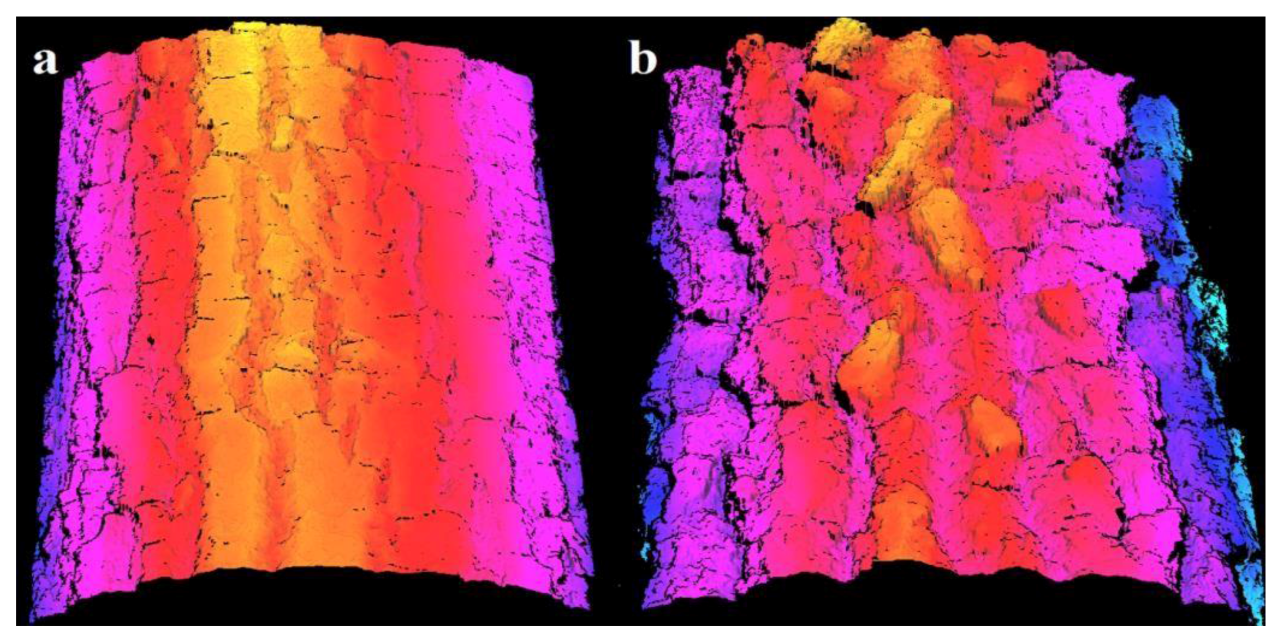
Figure 4 shows an image of the oak bark surface made from two samples. Sample A describes a bark at a height of 15 m while Sample B describes bark at a height of 1.5 m. Images of all the species presented in Figure 1 were made in an identical manner. The three-dimensional image of the surface shown in Figure 4 was subjected to a pre-treatment with the aim of eliminating interference and filling in data in areas that were not described; data was missing either due to light occlusion or not being on the camera’s optical path. This is the first step in the analysis of the three-dimensional image and is used to remove distortions and prepare it for measurement tasks.

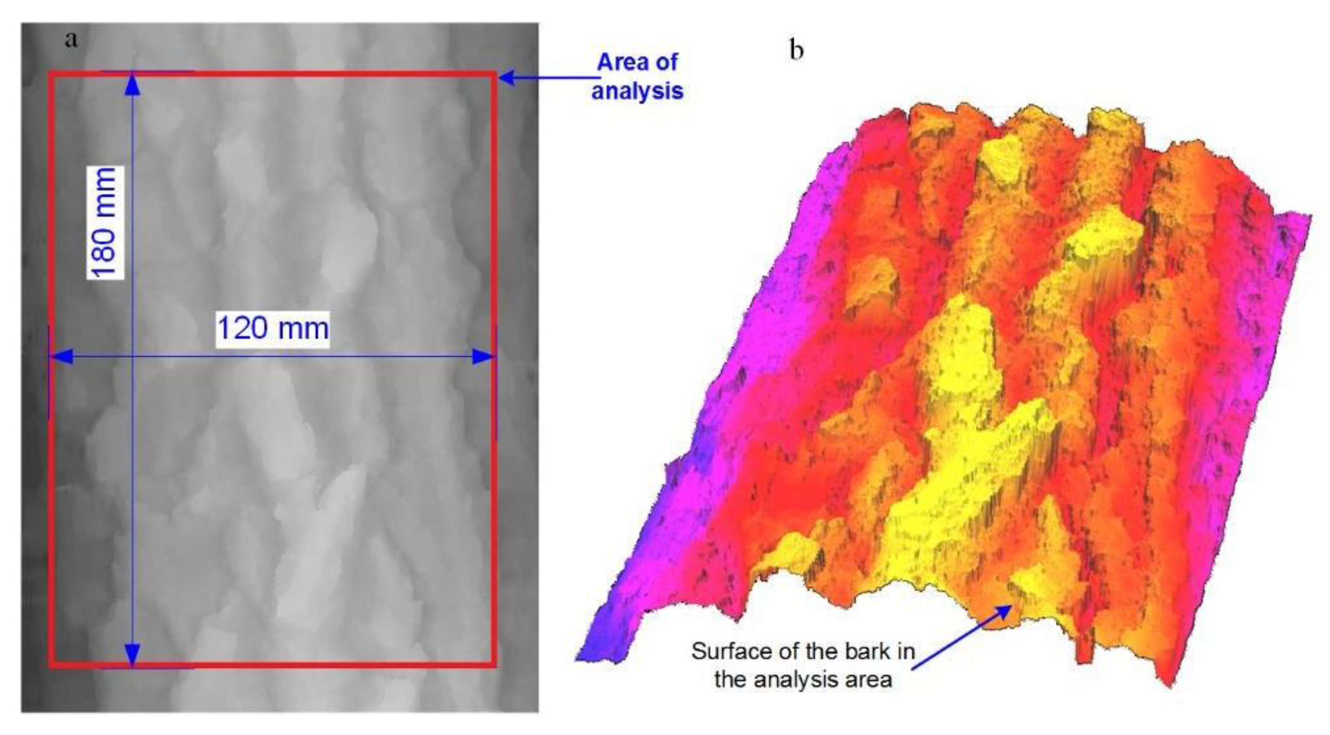
A control surface of 180 × 120 mm² was obtained as described using 900 profiles, each having 600 measuring points in width. Bark analysis of all examined species (Figure 5) was accepted for delineation of the shape of the bark surface. This surface serves as the unit area for facilitating the description of local bark parameters for one species at different heights of the tree trunk. It was also used for comparative measurements of different species. The shape and dimensions of the area are shown in the figure below.

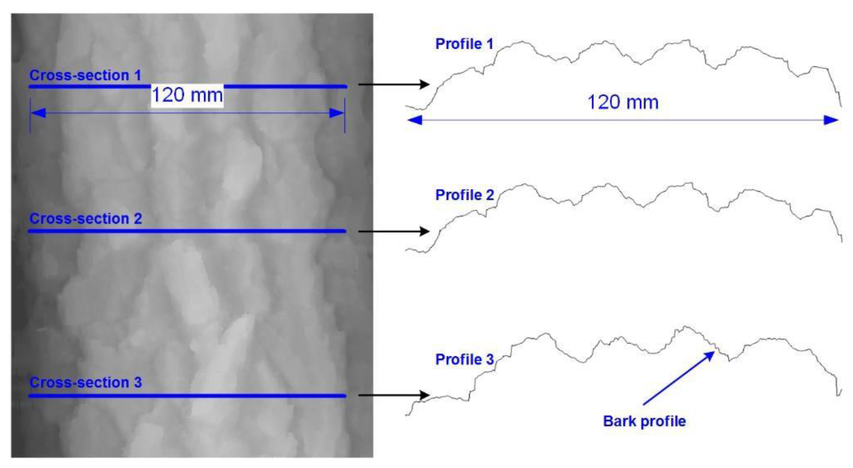
The analyzed area of the bark is presented in Figure 5b. A set of sections describing the height of bark profile in a cross-section transverse to the tree trunk axis (with a resolution of 0.2 mm) is assigned for this surface. The method of analyzing sections on a three-dimensional image and examples of height profiles are presented in Figure 6.

For each section described for the test sample, a curve describing the bark reference profile enabled the determination of a reference radius for the bark surface. This curve uses an estimator in the form of a function described below.

Z = b₀ + b₁X + b₂X²

(5)

where: Z—reference profile; X—section length; b₀, b₁, b₂—equation parameters.

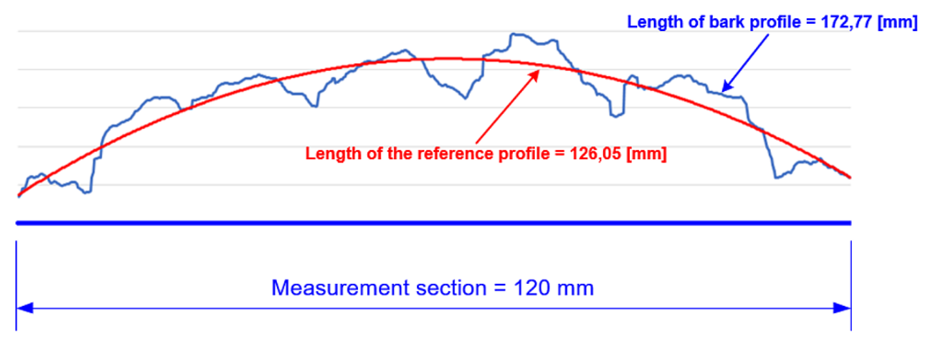
Upon determination of the reference profile seen in Figure 7, its length and length of the actual bark profile are determined on a measurement section 120 mm in length. This corresponds to the width of the bark surface analysis area.

A coefficient relating the length of the actual bark profile to the length of the reference profile (W_L) may be used as the exit parameter for the estimation of bark shape at the selected measurement section. For measuring section 120 mm, the coefficient is:

$${\mathrm{W}}_{\mathrm{L}\left(120\right)}=\frac{{\mathrm{L}}_{\mathrm{K}}}{{\mathrm{L}}_{\mathrm{R}}}=\frac{172.77}{126.05}=1.37$$

(6)

where L_R is the length of the reference profile and L_K is the length of the actual bark profile.

This coefficient describes “bark porosity”; for smooth bark, it assumes values close to 1. The value of the coefficient rises in cases where bark has a higher porosity. It can be used to evaluate the bark surface in a single profile and to determine the average value of the coefficient for 900 profiles made in the measurement area on a 3D image.

$${\overline{\mathrm{W}}}_{\mathrm{L}\left(120\right)}=\frac{{{\displaystyle \sum }}_{\mathrm{i}=1}^{900}{\mathrm{W}}_{\mathrm{L}\left(120\right)}}{900}$$

(7)

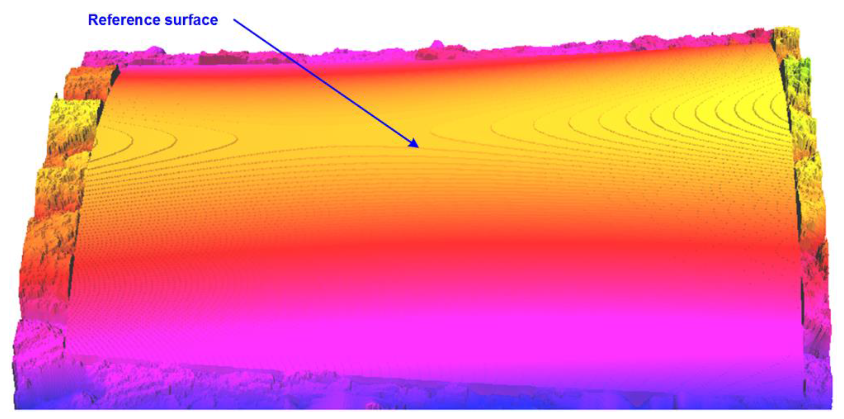
Analysis of subsequent profiles helps to determine reference surfaces for the whole area selected for analysis. An example of a reference surface is shown in Figure 8.

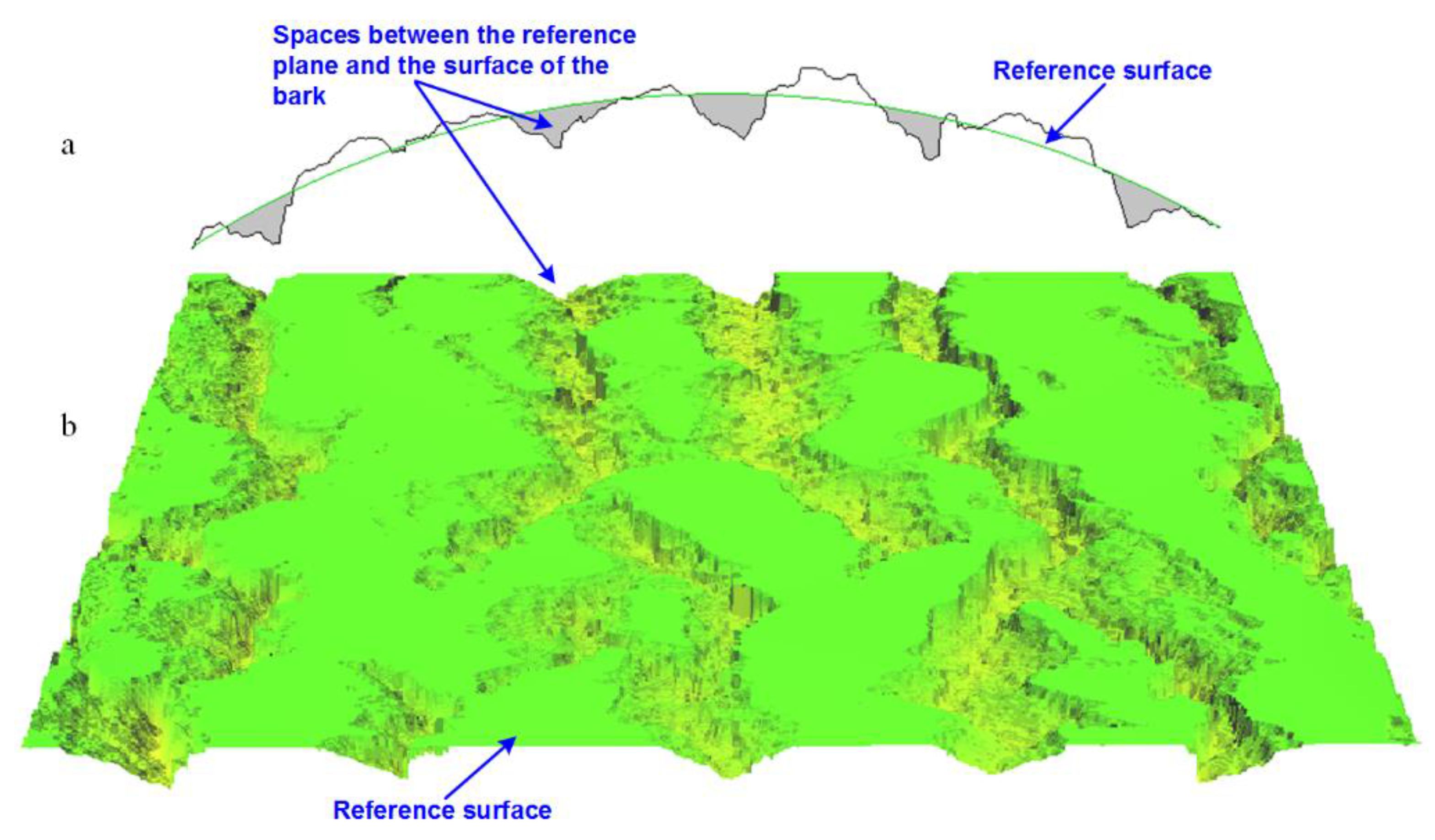
The reference surface was then used to designate the volume of space defined between the reference surface and the actual bark surface area. These spaces are marked on a selected cross-section shown in Figure 9a. Figure 9b shows the reference surface transformed into a plane with visible grooves corresponding to the defined spaces.

Another parameter put forward for evaluation of the bark surface is the volume factor (W_V); this is defined as the volume of the space between the reference plane and the surface of the bark. This factor is calculated as the quotient of the determined volume and the measurement area. Its formula is:

$${\mathrm{W}}_{\mathrm{V}180\mathrm{\times }120}=\frac{{\mathrm{V}}_{\mathrm{K}}}{{\mathrm{P}}_{180\mathrm{\times }120}}$$

(8)

where V_K is the space located between the reference plane and the surface of the bark and P_180×120 is the surface area of the measurement area.

The coefficient is expressed in millimeters and defines the mean height of the water-accumulating space calculated relative to the reference plane.

The bark area of a tree trunk with a radius of 150 mm and a height of 1000 mm was determined from the formula

$$\mathrm{Pp}=2\times \mathsf{\pi }\times \mathrm{R}\times \mathrm{h}=2\times \mathsf{\pi }\times 150\times 1000=\mathrm{942,477.8}\left({\mathrm{mm}}^2\right)$$

(9)

3. Results

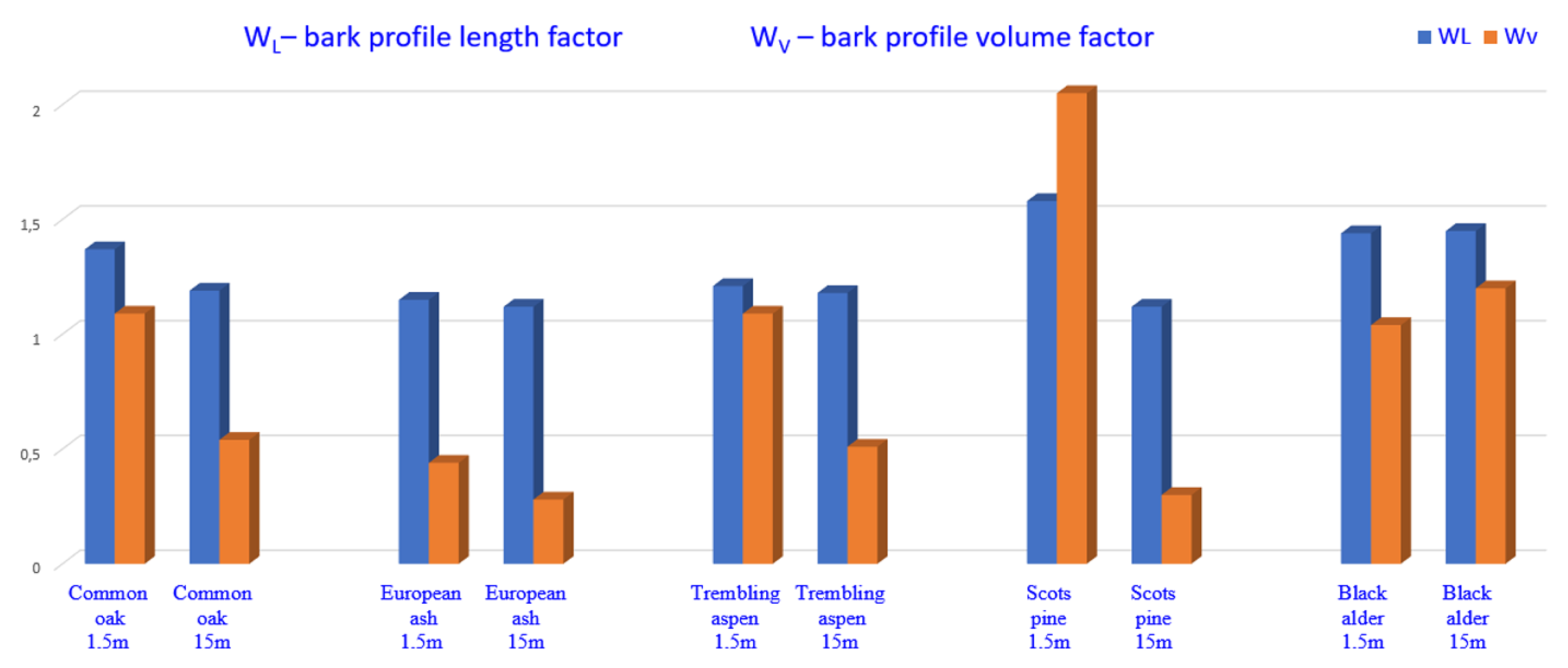
The designed automated system was practically applied for the calculation of developed indices for bark samples collected from five forest-forming tree species: common oak, European ash, trembling aspen, Scots pine, and black alder (Figure 10). In order to analyze intra-specific variability, values of W_L and W_V were calculated from samples collected from each individual species. Samples were taken from the lower and middle part of the tree stem at heights of 1.5 and 15 m above the ground level, respectively (Figure 10).

Obtained results indicate inter- and intra-specific differentiation of W_L and W_V factors. In the case of European ash, trembling aspen, and black alder, values of W_L factors calculated for samples taken at 1.5 and 15 m were nearly equal. In the case of the common oak, the W_L factor calculated for the sample at 1.5 m is larger than that calculated for the sample collected at 15 m. The largest difference between W_L factors calculated for bark samples from the lower and middle parts of the tree was observed in the Scots pine (Figure 10); the value of W_L calculated for the sample taken at 1.5 m is about 45 % lower than that calculated from the sample taken at 15 m.

Larger inter- and intra-specific variability was observed in the case of the W_V factor, which describes the volume of the space located between the reference plane and the surface of the bark (Figure 10). The lowest values of W_V were observed in the case of European ash, whereas Scots pine and black alder are characterized by the largest W_V factor. In the case of four analyzed tree species, values of the W_V factor calculated for samples collected at 1.5 m were at least two times larger than their counterparts collected at 15 m. However, we found one exception to this rule: in the black alder, values of the W_V factor calculated from the lower part of the tree were slightly lower than that from the middle part of the tree (Figure 10).

A comparison of the W_L and W_V factors at the heights of 1.5 and 15 m shows that black alder has a comparable BM along the entire trunk. Simultaneously, black alder is characterized both by a high bark profile length and bark profile volume factor. This suggests that its bark is one of the most water-retaining of the analyzed tree species.

Large intra-specific differentiation of W_V factors calculated for the lower and middle tree parts in species which were also characterized by low intra-specific differentiation of W_L values indicate a different meaning of these BM characteristics. This suggests that, for a more precise characterization of BM, both W_L and W_V factors should be used simultaneously.

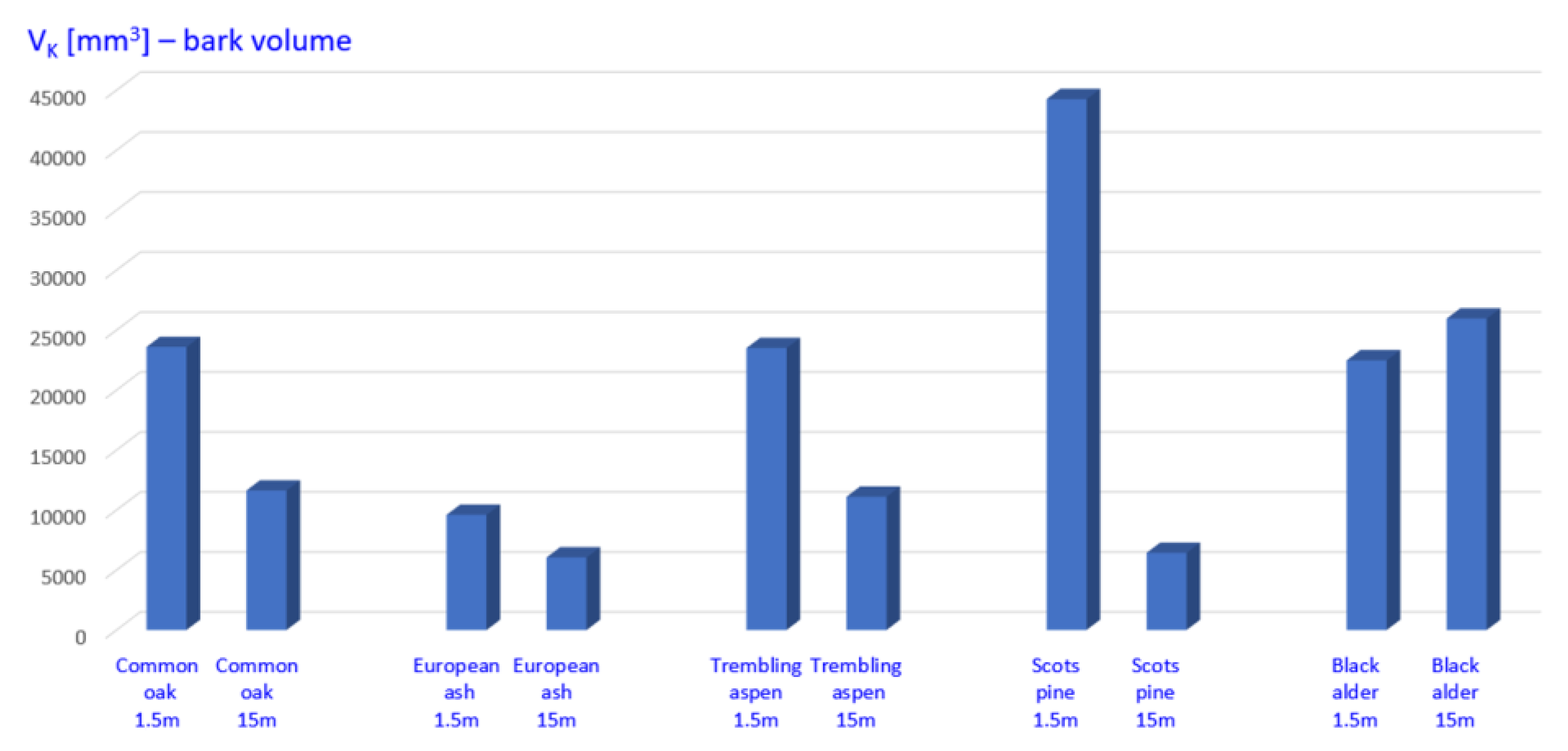
The water interception potential of the bark surface of analyzed tree species at their lower and middle parts was approximated using the given volume (in mm³) of the space between the reference plane and the surface of the bark (Figure 11).

For this example, volumes of the space between the reference plane and the surface calculated for the Scots pine at a height of 1.5 m (i.e., V1.5), a length of 1 m, and a diameter of 300 mm were counted as a product of 43.62 and 44,257.31. This was equal to 1.931 L. The volume of the bark on the trunk of the Scots pine at a height of 15 m (i.e., V15), a length of 1 m, and a diameter of 300 mm is 0.280 L. This indicates that while the bark at the lower part of the Scots pine stem has the largest water interception potential, the water interception potential of the bark at the upper part of the Scots pine (characterized by V15) is simultaneously one of the lowest of all analyzed species (Figure 11).

4. Discussion

The designed automated system allows for the fast calculation of proposed factors characterizing BM variability. Therefore, it could be useful in the analysis of both inter- and intra-specific differentiation and the characterization of BM for different purposes. Measurement of the actual area of the bark surface usually requires carrying out physical cuts of each bark sample. Then, the cuts made are scanned, multiple measurements are performed, and calculations are made. These calculations become the basis of the coefficient. When analyzing the current development of methods of bark description (e.g., BM), it should be noted that the described methods of preparing the physical cuts of bark in [4] are very time consuming. Measurement of the bark profile using a sensor and positioning rings mounted on the tree trunk, as described in the work of [23], constitutes a significant improvement of the work. It makes it possible to evaluate one bark profile (or BM) from selected tree trunk cross-sections, but requires change of the position of the coupling device on the tree trunk to determine the next profile. Studies have shown that it would be useful to compare the mounted bark profile on successive profiles spread evenly along the tree trunk [36]. Also, Levia and Herwitz [14] noticed that estimation of bark properties and water capacity in a laboratory could possibly differ from field values because the nature of wetting was unnatural. The presented method would be useful in analyzing bark cross-sections, as well as measuring BM parameters along the trunk axis or on any cross-section on the bark surface also in the tree stand. One limitation of the methods applied to date is the need to manually set the position of the measuring device on the examined objects to record the next BM.

The solution proposed in this paper takes into consideration the possibility of registering several hundred to several thousand bark profiles, thus facilitating the automation of constructing the bark’s three-dimensional image. In this paper, the resultant imaging of the bark surface shall be referred to as the “control surface”. The solution presented makes it possible to set required parameters of bark imaging resolution and 3D image acquisition without the need for making cross-section cuts and changing the mounted position of the measuring unit. The paper presents a system for analyzing a bark surface measuring from 120 to 180 mm at a resolution of 0.2 mm.

An unquestionable advantage of this solution is the ability to control the parameters of the measurement resolution. It also allows for the control of surface dimensions that facilitate assessment of BM on larger or smaller areas of the bark surface, depending on the requirements placed on the individual species or the age of the trees. This surface allows the BM to be evaluated on a plane perpendicular to the trunk axis, as well as on any cross-section on the control plane.

The use of three-dimensional image analysis for the evaluation of bark surfaces is a new technology that allows for fast, automatic determination of bark surface morphology features using the derived coefficients. A three-dimensional image of the bark is recorded using a triangulation video system, then the image is subjected to a pre-treatment to prepare it for measurement procedures. Subsequently, modifications and measurements of proposed coefficients are carried out in less than a second. Data describing the bark and its three-dimensional image are sent to database systems to help in the comparative assessment of results from one species, as well as implementation of interspecies assessments. Analysis of three-dimensional images of bark surfaces could be expanded to include additional parameters based on the analysis of the bark profile both on selected cross-sections and on the entire bark surface in selected measurement areas.

Determining the properties of bark, such as microrelief, is inherently meaningful from an environmental point of view because these greatly influence the proportion of intercepted rainfall [37]. It seems that the volume of the space located between the reference plane and the surface of the bark could be a good estimate of the potential water retention by tree bark, which is frequently analyzed in water balance analysis [38,39,40]; however, this needs to be verified experimentally. W_V could also be used in the context of a phytoremediation [41] and technical properties of bark [42,43]. The developed method of BM characterization could be also used in the study of ecology and in modelling the distribution potential of corticolous lichens and bryophytes. These are both partly governed by bark texture [15] and bark water storage capacity [19].

The obtained results indicate both inter- and intra-specific differentiation of BM characteristics. This indicates the need to take the large variability of BM indices along the stem into consideration. Moreover, it could be expected that BM characteristics vary with the age and dimensions of the tree, and the site conditions [44,45,46].

Therefore, with regards to hydrological modelling, models that describe BM characteristics along the individual species’ stem and that also take into account possible differences resulting from tree age and site conditions are necessary in improving the assessment of water interception by tree bark [19]. Livesley et al. [37] studied the impact of bark type on interception and found that there were less frequent and less total stemflow in rough bark as compared to smooth bark. Our calculations indicate that the volume of the space between the reference plane and the surface of the bark in the lower part of the Scots pine trunk is seven times larger than that in the upper part of the trunk. This indicates a large variability in water interception potential and other ecophysiological functions of the bark surface in different parts of the tree stem. Our developed method of BM characterization could fill the gap between the surface properties of bark and their effect on hydrological parameters. However, laboratory experiments are necessary to directly estimate the water interception potential by the bark area characterized by the given W_V factor. For such an experiment, direct values of water interception potential corresponding to the relevant W_V values should be estimated. Also, further research is necessary on the determination of bark’s ability to capture pollutants and on the effect of BM characteristics on other ecophysiological functions.

5. Conclusions

The presented bark scanning method and microrelief metrics improve spatial measurement capabilities in forests. The presented method of bark surface morphology analysis based on 3D images contributes to acquiring many more measurements and tests encompassing spatial measurements. The developed prototype of the vision system may also be used as a portable device. This makes it possible to use it in field measurements of bark surface morphology coefficients without the need for the laborious collection of samples. A portable automatic vision system could also ease the comprehensive assessment of the variability of bark surface morphology indicators depending on the location on the stem, thickness of the stem, age of the trees, and site conditions. It could also ease the description of these factors by using the form of models. This would contribute to a better understanding of the role of bark as a reservoir for water; this, in turn, is of crucial importance in the quantitative description of water interactions by forest ecosystems and other bark ecophysiological functions. Obtained results indicate inter- and intra-specific differentiation of BM characteristics.