Evaluating the Performance of High-Altitude Aerial Image-Based Digital Surface Models in Detecting Individual Tree Crowns in Mature Boreal Forests

Abstract

Height models based on high-altitude aerial images provide a low-cost means of generating detailed 3D models of the forest canopy. In this study, the performance of these height models in the detection of individual trees was evaluated in a commercially managed boreal forest. Airborne digital stereo imagery (DSI) was captured from a flight altitude of 5 km with a ground sample distance of 50 cm and corresponds to regular national topographic airborne data capture programs operated in many countries. Tree tops were detected from smoothed canopy height models (CHM) using watershed segmentation. The relative amount of detected trees varied between 26% and 140%, and the RMSE of plot-level arithmetic mean height between 2.2 m and 3.1 m. Both the dominant tree species and the filter used for smoothing affected the results. Even though the spatial resolution of DSI-based CHM was sufficient, detecting individual trees from the data proved to be demanding because of the shading effect of the dominant trees and the limited amount of data from lower canopy levels and near the ground.

1. Introduction

An individual tree is the basic element of traditional forest inventory, as forests are composed of individual trees and forest stands constitute larger forested areas. Hence, information on individual tree attributes (such as volume) is retrieved first, and tree-level attributes are then compiled for stand-level forest inventory attributes. This requires that all trees within the area of interest be observed and measured. Airborne laser scanning (ALS) provides accurate 3D information and enables the development of detailed maps of ground elevation and characterization of forests. In contrast to many remote-sensing data sources, ALS is spatially detailed (high spatial resolution) and captures the height of trees and other vegetation. Heights of individual trees or canopy density can be accurately deduced with ALS. ALS is already utilized in operational forest inventory for predicting stand-level forest inventory attributes via the area-based approach (ABA) [1,2,3,4]. In the ABA, the area of interest is tessellated into grid cells, and relations between cell-wise ALS-derived point metrics and field-measured forest inventory attributes are searched. Based on the relationships found, forest inventory attributes can be predicted for all grid cells. Compared to traditional stand-wise field inventory (SWFI), ABA has provided more accurate estimations of forest inventory attributes [5]. However, ABA does not provide tree-level information needed in detailed forest management (e.g., diameter distribution), and the accuracy of estimations regarding the number of trees or timber assortments is similar to SWFI [1,6].

The development of laser scanners has enabled the identification of individual trees from the ALS data. During the last 10–15 years, techniques for detecting single trees have been developed and tested (e.g., [7,8]), but have yet to be adopted in operational forest inventory. In the past, single-tree-based approaches were presumed to perform best with dense (at least five points per m²) ALS data. Kaartinen and Hyyppä [7] analyzed nine different methods (algorithms) based on the smoothed surface model (i.e., canopy height model, CHM) from ALS data for detecting individual trees in two test sites. The results showed that preprocessing of ALS data influenced the accuracy greatly, whereas changes in the point density between 2 and 8 points/m² did not affect the detection rate of the trees. Vauhkonen et al. [8] tested six different algorithms from which four utilized CHM for detecting single trees in varying forest conditions. The algorithms performed similarly and differences between detection rates (from 45.2% to 100.7%) were more affected by forest structure (e.g., tree density and clustering) than different algorithms. Omission errors (i.e., trees not detected, usually suppressed under dominant canopy layer) varied between 30.6% and 61.1%, whereas commission errors (i.e., trees detected from ALS but not linkable to any field tree) varied from 6.9% to 39.4%. Although ALS-based individual tree detection (ITD) has proven to provide accurate estimates for logging recovery in mature single-tree-species stands [9], reliable tree detection in varying forest conditions still remains challenging [8,10,11,12]. One of the challenges is to detect suppressed trees more accurately. Maltamo et al. [13] used the Weibull distribution to detect suppressed trees and were able to decrease the relative root-mean-square error (RMSE) from 74.4% to 49.2% for the number of stems. Hyyppä et al. [14] employed last returns in identifying suppressed trees and were able to improve the detection accuracy by 6%.

Processing a CHM usually includes smoothing in order to reduce height variation within tree crowns (e.g., one crown can include many tree tops, especially with deciduous trees) and improve detection accuracy. A Gaussian filter is commonly applied for smoothing the CHM before delineating individual tree crowns by segmenting it [7,8,15]. There are several methods for segmenting the CHM, but most of them are based on finding local maximum values and expanding segments by adding pixels to them if they meet the criteria (e.g., neighboring pixels have lower height values in “pouring” analysis) [15,16,17,18]. The excess segments are primarily a consequence of the occurrence of several height peaks within individual tree crowns. Smoothing the CHM reduces the number of created segments, but on the other hand, also makes the smallest crowns near larger ones disappear. In some studies, this problem has been minimized by using adaptive Gaussian filters (e.g., [11,19]).

Moreover, utilization of aerial imagery in environmental mapping is a longstanding tradition. Aerial imagery has been widely utilized in forest inventory, especially in the identification of tree species [20,21,22,23,24,25]. Digitalization of aerial photography and developments in image-matching algorithms have increased the interest in 3D point clouds and surface models based on digital stereo imagery (DSI). The interest in utilizing stereo or multi-view DSI for predicting forest inventory attributes [26,27,28,29,30] is also increasing, as the temporal resolution of 3D remote sensing data can be improved with it. Photogrammetric point cloud generation by digital image-matching requires that the same object be viewed in at least two different images. The current image-matching strategies (e.g., semi-global matching, SGM) are capable of generating dense point clouds [31]. The choice of image-matching algorithm affects the accuracy of the generated point clouds to some extent, especially in forests [28]. Although predicting forest inventory attributes has also been possible solely with DSI, many studies have employed a combination of DSI and ALS, where ALS has provided the digital terrain model (DTM) and the digital surface model (DSM) has been generated from DSI-based point clouds (e.g., [3,32]). The capability of DSI to characterize forest canopy is poorer compared to ALS because DSI cannot really penetrate through the canopy [33]. Thus, utilizing the available ALS-based DTM is justified. The abovementioned studies applying DSI have mainly focused on predicting the forest inventory attributes at a plot or grid level comparable to ABA [34]. However, recent research has also utilized individual tree detection from DSI [35,36,37]. St-Onge et al. [35] compared tree detection and tree-level height estimates based on DSI to ALS, and obtained similar results with both data sets. They also highlighted the capability of DSI in species recognition, compared to ALS, when spectral values are included in addition to height information gained from DSI-based point clouds. Additionally, Tompalski et al. [37] compared tree detection based on ALS to DSI and concluded that the quality of data affects the results more than the methodological approach used. Rahlf et al. [36], on the other hand, used DSI to compare ITD and ABA in estimating forest inventory attributes and obtained similar results with both approaches.

Information on forest resources for forest management planning has been acquired in ten-year cycles in Finland. Nowadays, ALS data are utilized in producing forest resource information with ABA, but due to the cost of ALS data, the data acquisition for forest management planning in shorter intervals may not be feasible. The advantage of DSI, compared to ALS, is higher cost efficiency—especially in large areas. Therefore, digital aerial images could be available more often (e.g., every three years). One of the challenges associated with ALS has been recognizing tree species reliably; thus, combining ALS data and aerial images has been proposed for the estimation of stand-level forest inventory attributes [2]. If individual trees can be identified and detected from DSI data with similar or improved accuracy compared to ALS, it could enhance the identification of tree species. Using DSI-based 3D point clouds and spectral data, St-Onge et al. [35] reported very promising results on detection and species classification of individual tree crowns. In addition, a combination of ALS and DSI could be a solution for species recognition: Holmgren et al. [38] achieved 96% classification accuracy when identifying pine, spruce, and deciduous trees.

The objective of this study was therefore to investigate the capability of DSI in detecting individual trees in mature stands of managed forests with varying main tree species. The emphasis was to test how filtering DSI-based CHM with various methods affects not only the accuracy of identifying the trees but also the estimates of arithmetic mean height (henceforth, mean height) under different tree-species compositions. Thus, our hypothesis was that using DSI-based CHMs in ITD, the dominant tree species affects the selection of optimal filter, and detecting single trees is more accurate in conifer-dominated stands. National DTM based on ALS was used in normalizing DSI-based DSM in CHM generation.

2. Materials and Methods

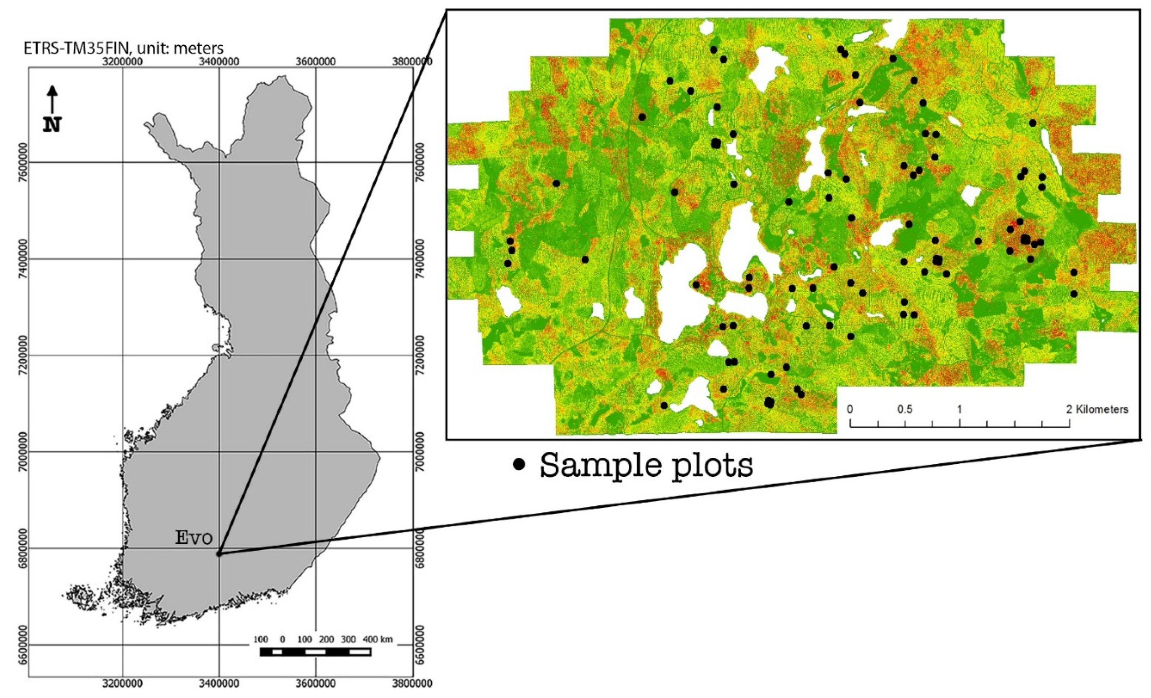
2.1. Test Site

The study area of 5 km × 5 km is located in Evo, southern Finland (61°11′24′′ N, 25°06′36′′ E, Figure 1). It belongs to the southern boreal forest zone and contains approximately 2000 ha of managed boreal forest. The average stand size is slightly less than 1 ha. The area consists of a mixture of forest stands, varying from natural to intensively managed forests. The elevation of the area varies from 125 m to 185 m above sea level. The dominant tree species are Scots pine (Pinus sylvestris L.) and Norway spruce (Picea abies (L.) H. Karst), making up 40% and 35% of the total volume, respectively. The proportion of all deciduous trees together is 24% of the total volume.

2.2. Field Data

The field data included 39 plots (32 m × 32 m, 1024 m²) from mature forests with varying dominant tree species. The field campaign was carried out in the summer of 2014. Before the actual field measurements, terrestrial laser scanning (TLS) measurements were conducted, and stem maps (i.e., location and identity code for each tree) were created based on the TLS data. These stem maps were used to locate the trees in the field plots. Locations of the missing trees were added to the stem maps based on four field measured distances and directions. All of the trees that were not found during field measurements but appeared in the stem maps were deleted from the final stem maps. From the sample plots, all trees with diameter-at-breast-height (DBH) of over 5 cm were measured with steel calipers in two perpendicular directions, and the mean of the two readings represented the DBH. The height of the trees was also measured using an electronic hypsometer. The tree volumes were calculated with standard Finnish models [39]. The models used tree species, DBH, and height as input variables. The forest inventory attributes for sample plots were obtained by averaging or adding up the tree-level data. The field data was limited to the trees with at least some timber value. Hence, only the trees taller than 14 meters were used in this study when calculating the plot-level arithmetic mean heights. Trees of this size were mostly visible from above, but the visibility varied with the species composition and spatial distribution of the trees.

Sample plot locations were calculated using the geographic coordinates of six reference points inside the plots. The positions of the reference points were measured using a combination of differential GPS (Trimble R8) and a total station (Trimble 5602). The total station was oriented using two GPS locations from an opening (e.g., a road) adjacent to the plot and away from dense cover. The reference points were positioned using distances and angles from the total station. Plot position was further adjusted manually using ALS data. In this procedure, the locations of all trees on the stem map were used to help find the true location of the plot in the ALS point cloud. The plot was shifted and rotated so that the tree locations within the map aligned properly with the point cloud.

The field plots were further divided into subgroups based on the tree species, accounting for 70% or more of the basal area—i.e., the dominant species. The classes were defined as described in

Table 1. Definitions of study subgroups.

Subgroup	Group Description	n
Pine	Plots with pine representing over 70% of the basal area	12
Spruce	Plots with spruce representing over 70% of the basal area	15
Deciduous	Plots with deciduous trees representing over 40% of the basal area	3
Mixed	Mixed plots with none of the species representing over 70% of the basal area	12
Total	All plots	39

. One of our aims was to closely examine the plots with the most deciduous trees. In order to do so, the classification limit of the deciduous subgroup was reduced from 70% to 40% of basal area. However, the deciduous plots are also counted as mixed plots (hence, in Table 1 the number of deciduous plots is given in brackets). The descriptive statistics of all subgroups are presented in

Table 2. The descriptive statistics of 39 sample plots of 32 m × 32 m used in this study. DBH: Diameter-at-breast-height.

		Minimum	Maximum	Mean	Standard Deviation
Pine	Mean height (m)	21.4	32.1	25.8	3.6
	Mean DBH (cm)	26.3	46.4	30.8	6.0
	Basal area (m2/ha)	17.3	40.3	26.7	7.1
	Volume (m3/ha)	164.5	518.4	300.0	109.4
	Plot density (trees/ha)	391	1035	565	201
Spruce	Mean height (m)	25.4	33.4	29.2	2.6
	Mean DBH (cm)	26.0	42.1	33.9	5.4
	Basal area (m2/ha)	22.1	38.9	32.8	5.1
	Volume (m3/ha)	242.6	484.9	390.8	75.0
	Plot density (trees/ha)	342	879	585	159
Deciduous	Mean height (m)	23.1	31.6	27.1	4.3
	Mean DBH (cm)	26.6	32.9	28.9	3.5
	Basal area (m2/ha)	25.6	39.6	31.9	7.1
	Volume (m3/ha)	257.9	369.2	305.2	57.5
	Plot density (trees/ha)	547	2217	1218	882
Mixed	Mean height (m)	23.1	31.6	27.4	2.7
	Mean DBH (cm)	26.6	41.6	33.4	5.0
	Basal area (m2/ha)	15.2	43.2	33.1	8.0
	Volume (m3/ha)	177.7	508.2	349.1	96.4
	Plot density (trees/ha)	342	2217	909	482
Total	Mean height (m)	21.4	33.4	27.6	3.2
	Mean DBH (cm)	26.0	46.4	32.8	5.5
	Basal area (m2/ha)	15.2	43.2	31.0	7.2
	Volume (m3/ha)	164.5	518.4	350.0	98.4
	Plot density (trees/ha)	342	2217	678	335

.

2.3. Aerial Images and Processing into Digital Surface Model

The aerial images of the Evo area were acquired on 22 May 2014 by the National Land Survey of Finland (NLS) using a Z/I Imaging Digital Mapping Camera. The image block was comprised of two flying strips, both consisting of 12 images, resulting in a total of 24 images. The forward and side overlap of the pictures were 80% and 64%, respectively. The flying altitude was approximately 5000 m above the mean ground level, leading to a ground sample distance (GSD) of approximately 50 cm. The width of an image strip was 6.9 km, and the distance between adjacent flight lines was 2.5 km. The imagery had exterior orientation values that were used as an initial orientation when importing the images into BAE Systems Socet Set software (San Diego, CA, USA). The final orientation was based on automatic tie points and 40 interactively measured ground control points. The ground control points were derived from elevation model and orthophotos of the NLS. Three radial distortion parameters were solved with on-the-job calibration. The root-mean-square error (RMSE) values of the adjustment were 0.266 m (X), 0.400 m (Y), and 1.187 m (Z).

Socet Set was also used for extracting the 3D information from the images. The calculation of triangulated irregular network (TIN)-type surface models was carried out with the NGATE (Next Generation Automatic Terrain Extraction) module of the Socet Set software bundle, using a matching strategy suitable for forestry applications. NGATE is based on correlation matching using a multiresolution image pyramid. An image correlation window size of 11 × 11 pixels was used in each image pyramid level, and steep height variations as well as large search distances were allowed in order to obtain good reconstruction of the forest canopy. Extraction of DSM was done for each stereo model of consecutive images in the same strip, but inter-strip stereo models were not used in the calculation. The DSMs, with a resolution of 0.5 m, were exported in ASCII format either with Socet Set (V4.1) or Socet GXP (V5.6) software (BAE Systems, San Diego, CA, USA) and transformed into GeoTIFF format using Matlab (2015b) (MathWorks, Inc., Natick, MA, USA). National ALS-based DTM (resolution of 2 m) obtained from NLS was used to normalize DSM into CHM.

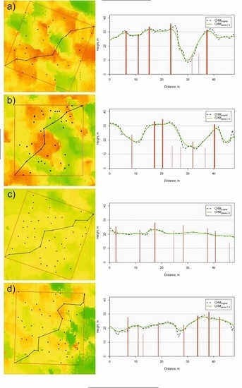
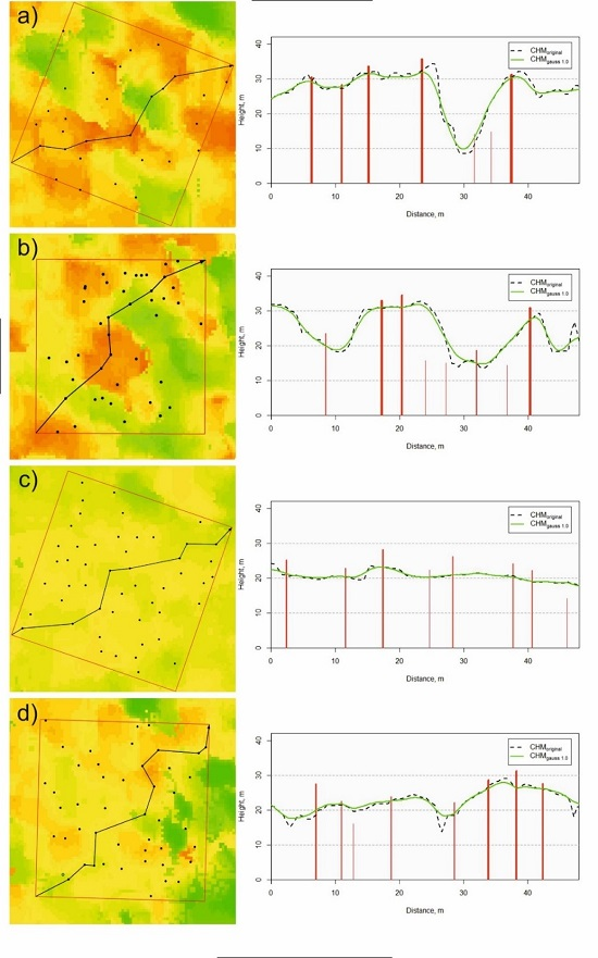
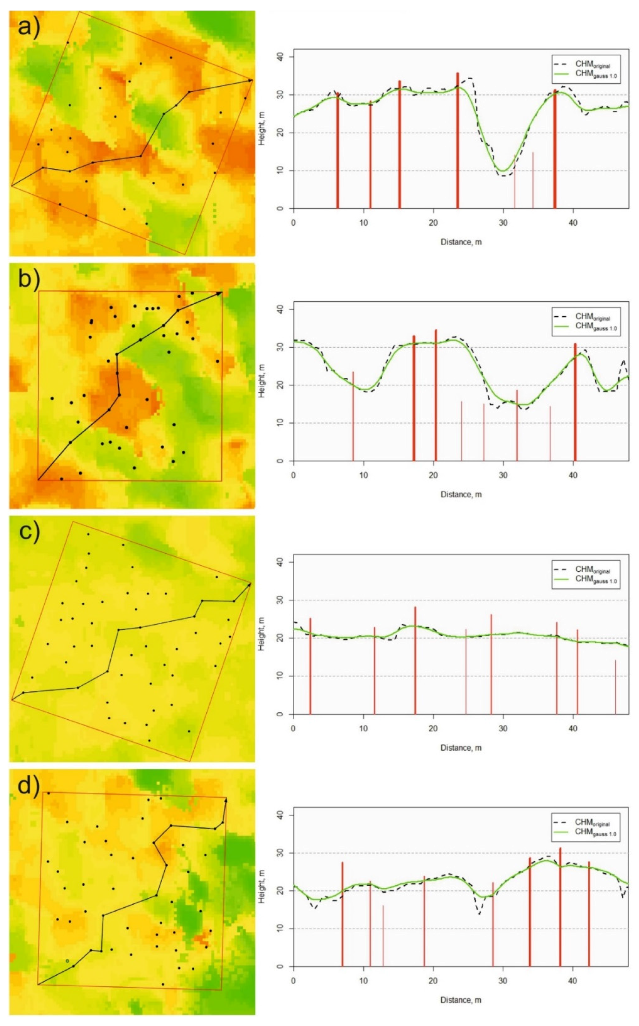
2.4. Quantifying and Visualizing the Effects of CHM Preprocessing

To determine the effects of CHM preprocessing, altogether 13 different filters were tested. The tested filters included three filters with preset weights and a Gaussian filter with varying sigma determining the magnitude of the filtration. The filters with preset weights utilized 3 × 3 pixel windows—i.e., kernels. In Filter_low (Equation 1, adopted from [40]), a moderate relative weight was given to the central pixels, whereas in Filter_high (Equation 2, adopted from [7]), the weight given to the central cell was higher. In addition to the two, a simple 3 × 3 pixel mean filter was tested. Using the Gaussian filter, the sigma values between 0.1 and 1.0 were tested. The size of the resulting filters varied from one pixel (sigma = 0.1) to 13 × 13 pixels (sigma = 1.0). As using sigma value 0.1 did not smooth the CHM (kernel size 1 × 1 pixel), the resulting CHM can be considered unsmoothed—i.e., the original DSI-based CHM.

$$Filte{r}_{low}=\frac{1}{16}\left[\begin{array}{ccc}1& 2& 1\\ 2& 4& 2\\ 1& 2& 1\end{array}\right]$$

(1)

$$Filte{r}_{high}=\frac{1}{28}\left[\begin{array}{ccc}1& 3& 1\\ 3& 12& 3\\ 1& 3& 1\end{array}\right]$$

(2)

The effects of smoothing were investigated throughout the study for all filtered CHMs.

The capability of DSI-based CHMs in describing the canopy structure of the forest and the effect of smoothing the CHMs were visualized by creating height profiles from four selected field plots: a pine-dominated, a spruce-dominated, a deciduous-dominated, and a plot with mixed tree-species. The profile lines were drawn using ArcMap 3D analyst (ESRI Inc., Redlands, CA, USA) from the lower left to the upper right corner of a plot, following the field-measured tree locations (Figure 2). Hence, the intersected tree tops should be visually detectable in the resulting height profiles.

2.5. Tree Delineation and Height Extraction

Individual crown segments were delineated from the CHMs using the watershed segmentation process (e.g., [15,17]). The process detects the local maxima of the CHM as starting points for the segmentation. If the eight connected pixels around the center pixel have lower CHM values, the center pixel is considered a local maximum. These points are considered to be the tree tops. The segment region is then extended from the local maximum by adding connected pixels with the same or lower height value to the region until a threshold value for minimum height is met. In this study, we used a height minimum threshold value of two meters. Three sets of crown segments were created by using the smoothed CHMs resulting from various filtering methods.

Because smoothing affects the extracted tree heights, the original, unfiltered CHM was used when deriving locations and heights for the trees extracted from the smoothed CHMs. The height and location were adopted from the maximum value of the unfiltered CHM inside each segment. If the maximum was a “plateau” consisting of several pixels, the location was determined as the mean location of the plateau pixels. The final tree candidates were chosen among the crown segments in terms of tree height. Focusing on mature trees, only crown segments with a CHM value (i.e., tree height) of at least 14 m were considered to represent actual trees.

The detected trees were divided into bins of 1 m based on their estimated height (i.e., maximum height of each segment) to generate separate height distributions, which were then compared to the reference distribution derived from tree heights based on field measurements.

2.6. Accuracy Assessment

The accuracy of ITD and estimated plot-level mean height were evaluated for all subgroups in terms of root-mean-square error (RMSE) and bias:

$$RMSE=\sqrt{\frac{{\sum }_{i=1}^n{(x_{ob{s}_i}-x_{ch{m}_i})}^2}{n}}$$

(3)

$$bias=\frac{{\sum }_{i=1}^n(x_{ch{m}_i}-x_{ob{s}_i})}{n}$$

(4)

where n is the number of plots, $x_{ch{m}_i}$ is the CHM-derived number of trees or mean height in the plot i, and $x_{ob{s}_i}$ is the observed number of trees or mean height based on field measurements in a plot I.

The accuracy of detecting individual trees was also analyzed through height distributions by comparing those based on CHMs smoothed with various filtering methods to the field-measured distribution. The differences between the measured and estimated height distributions were investigated through a relative error index (EI_rel), which has been used when defining accuracies of estimated diameter distributions [41,42,43] in the field of forest research:

$$E{I}_{rel}={\displaystyle \sum }_{i=1}^{k}0.5\left|\frac{f_i}{N}-\frac{{\widehat{f}}_i}{\widehat{N}}\right|$$

(5)

where k is the number of height classes, $f_i$ is the true number of trees in a height class i, ${\widehat{f}}_i$ is the predicted number of trees in height class i, N is the true total number, and $\widehat{N}$ the predicted total number of trees in the plot. The index was originally proposed by Packalén and Maltamo [44] and is based on Reynolds error index [45]. Compared to the Reynolds error index, in the $E{I}_{rel}$ the results are scaled between 0 and 1 by weighing them by 0.5. Thus, $E{I}_{rel}$ value of 1 indicates that the distributions do not overlap and value 0 indicates a perfect fit. The subgroup-level results were aggregated as mean values of plot-level results. The resulting index can be interpreted as the proportion of the detected trees that are classified incorrectly.

3. Results and Discussion

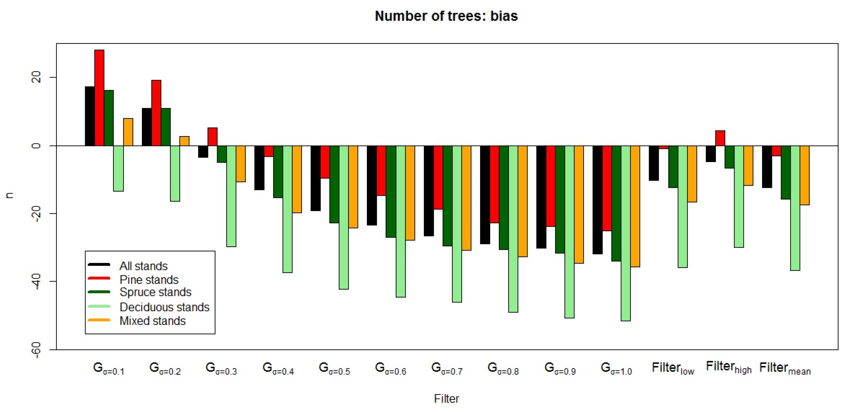
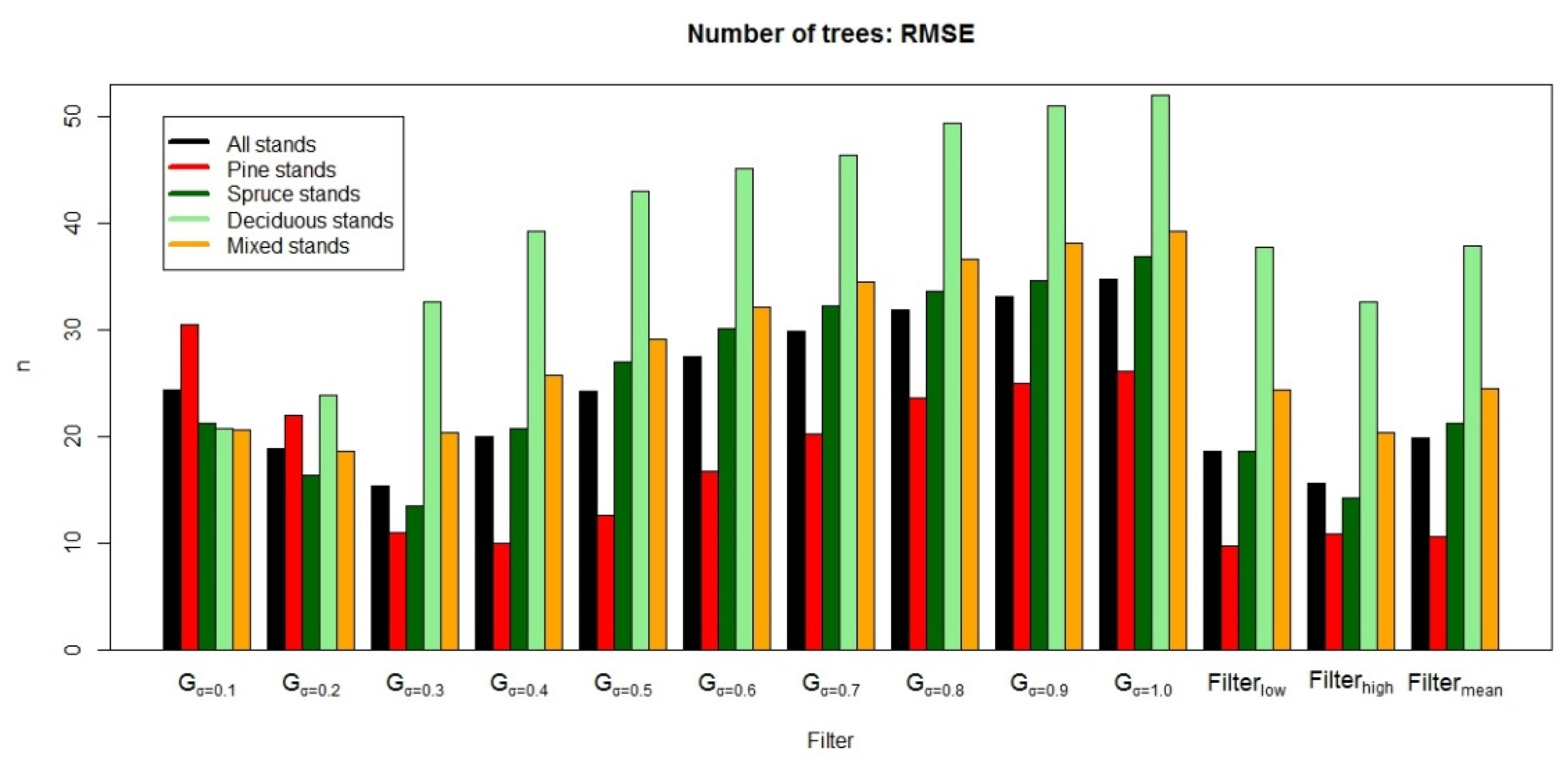
3.1. Tree Detection

When examining the effects of smoothing the DSI-based CHM, the differences in the number of detected trees were substantial. The number of trees in deciduous-dominated stands was underestimated (absolute bias between −52 and −13, and relative bias between −84.7% and −21.9%, respectively) when utilizing a Gaussian filter with all sigma values, whereas in all other stand types (pine- and spruce-dominated and mixed), sigma values of 0.1 and 0.2 produced overestimates (absolute bias between 3 and 28 and relative bias between 5.6% and 72.7%, respectively, Figure 3). The RMSE of number of trees in spruce-dominated stands was the lowest—i.e., 13 (30.3%)—with sigma value 0.3. In pine-dominated stands, it was 10 (25.6%) with sigma value of 0.4, whereas in deciduous-dominated stands, the lowest RMSE of 21 (33.9%) was achieved with sigma value of 0.1 (Figure 4).

When comparing bias and RMSE resulted with other filters, heavier filtering caused greater underestimation in deciduous stands (Figure 3), whereas in all other types of stands, lighter filters (i.e., Gaussian with sigma 0.1 and 0.2) resulted in overestimations of the number of trees. Filter_low resulted in an underestimation of only one tree in pine-dominated stands, whereas a Gaussian filter with sigma value of 0.2 and 0.3 reached the smallest bias in mixed and spruce-dominated stands, respectively (Figure 3). The RMSE of number of trees increased in deciduous stands when sigma increased in the Gaussian filter. Filters with a 3 × 3 pixel kernel size produced similar results to a Gaussian filter with sigma value of 0.4 in all stand types. The RMSE of number of trees was the highest in stands dominated by deciduous trees, except with Gaussian filter when sigma was 0.1, which produced the lowest accuracy in pine-dominated stands (Figure 4).

The average number of trees per hectare was clearly higher in deciduous plots compared to conifer-dominated and even mixed plots, which could be a reason for underestimations in the number of detected trees. The number of detected trees in various stand types is shown in

Table 3. The number of detected trees and detection rate (%) in brackets in various stand types when using different filtering methods. G stands for Gaussian filter.

Number of Detected Trees and Detection Rate (in Brackets)
	Pine		Spruce		Deciduous		Mixed		Total
	N	%	N	%	N	%	N	%	N	%
G0.1	803	(173)	908	(137)	143	(78)	650	(117)	2361	(140)
G0.2	697	(150)	829	(125)	134	(73)	585	(106)	2111	(125)
G0.3	529	(114)	592	(89)	94	(51)	425	(77)	1546	(92)
G0.4	426	(92)	436	(66)	71	(39)	317	(57)	1179	(70)
G0.5	349	(75)	324	(49)	56	(31)	264	(48)	937	(56)
G0.6	288	(62)	259	(39)	49	(27)	221	(40)	768	(46)
G0.7	241	(52)	222	(33)	45	(25)	183	(33)	646	(38)
G0.8	193	(42)	206	(31)	36	(20)	160	(29)	559	(33)
G0.9	180	(39)	190	(29)	31	(17)	139	(25)	509	(30)
G1.0	163	(35)	154	(23)	28	(15)	126	(23)	443	(26)
Filterlow	453	(97)	479	(72)	75	(41)	354	(64)	1286	(76)
Filterhigh	518	(111)	565	(85)	93	(51)	413	(75)	1496	(89)
Filtermean	428	(92)	428	(64)	73	(40)	345	(62)	1201	(71)
Field reference	465		665		183		554		1684

. The overall detection rates varied between 26% and 140% (i.e., 40% overestimation) between various filtering methods. The detection rates varied between 39% and 87% on average between stand types. However, it has to be borne in mind that as no matching between tree candidates and field-measured trees was made, even a 100% detection rate does not necessarily indicate a perfect detection: when plot averages are calculated, non-detection and over-detection (i.e., a single tree crown is split into several tree candidates) cancel each other out. One of the drawbacks of DSI-based CHM is the inadequate penetration of forest canopy, which results not only in lower detection rates of suppressed trees but also in overestimations of the number of trees due to an excess of crown segments. When employed in fine resolution CHMs, the number of segments resulting from the watershed procedure is often much larger than the actual amount of trees. The excess segments are primarily a consequence of the occurrence of several height peaks within individual tree crowns. Hence, the CHM is usually smoothed using a Gaussian filter [7,8,15], for example. Smoothing the CHM reduces the number of segments created, but on the other hand, also makes the smallest crowns near larger ones disappear. In some studies, this problem has been minimized by using adaptive Gaussian filters (e.g., [11,19]).

Vauhkonen et al. [8] compared four methods in delineating individual trees based on CHM, and reported an overall detection rate between 45.2% and 100.7% in varying forest conditions (i.e., Eucalyptus plantations, conifer- and deciduous-dominated managed forests), whereas Persson et al. [46] were able to detect 71% of the trees correctly. However, the detection rates in Kaartinen and Hyyppä [7] varied between 20% and 90%, which implies the extent to which the suppressed trees affect the overall detection rate. In a rather sparse single-storey forest, nearly all the trees could be detected, whereas in a dense forest with a lot of suppressed or clumped trees, the detection rate was considerably lower. However, mature stands were selected for this study to avoid this problem because our aim was to assess the effects of various filtering methods. Rahlf et al. [36] reported relative RMSE of 46% for detected trees with semi-automatic DSI-based ITD, whereas St-Onge et al. [35] presented relative difference between number of trees detected from DSI and ALS varying from −19.9% to 1.3% with different forest compositions. Tompalski et al. [37] were able to detect 74.1% of the trees with DSI-based CHM and local-maxima-search methodology for tree crown segmentation. We obtained the most accurate detection rate (97%) in pine-dominated stands with Filter_low, whereas the lowest detection rate (15%) occurred in deciduous stands using a Gaussian filter with sigma value 1.0. Overall, heavier filters produced lower detection rates in all stand types.

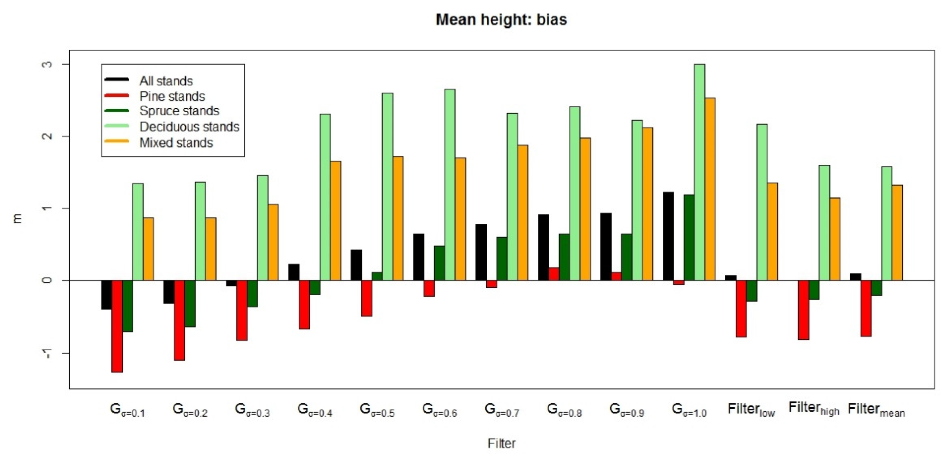
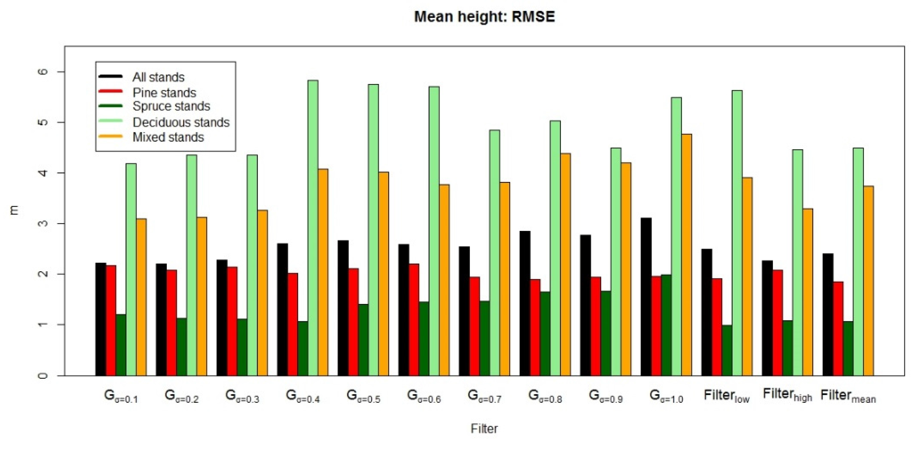
3.2. Estimated Mean Height

The smallest bias in plot-level mean height was obtained in pine-dominated stands with sigma values from 0.7 to 1.0—i.e., with the heaviest filtering (Figure 5). Bias in conifer-dominated stands varied when CHM was filtered more (i.e., the sigma values of the Gaussian filter increase). The effect of varying sigma value in RMSE of plot-level mean height when utilizing a Gaussian filter was more visible in deciduous and mixed stands than in conifer-dominated stands, especially where pine is the dominant tree species (Figure 6).

Mean height was overestimated in deciduous and mixed stands with all filtering methods, whereas in conifer-dominated stands it was mainly underestimated (Figure 5). In spruce-dominated stands, a Gaussian filter with sigma value 0.5 produced the smallest bias in mean height (absolute bias 0.1 m and relative bias 0.5%), but between mean filter and a Gaussian filter with sigma value of 0.4, the results were similar in spruce-dominated stands, where bias was approximately −0.2 m (0.8%).

When ignoring the differences between tree species specific subgroups, the RMSE of plot-level mean height varied between 2.2 m (9.3%) and 3.1 m (13.1%) in all stands when utilizing various filtering methods. The smallest RMSE (1.0 m, 4.0%) was obtained in spruce-dominated stands with Filter_low, whereas the highest RMSE (5.8 m, 28.3%) was found in deciduous stands when a Gaussian filter and sigma value 0.4 were employed (Figure 6). The largest errors seem to occur in deciduous and mixed stands, regardless of the filtering method. The difference between conifer stands and all other stands is more evident regarding plot-level mean height than the tree detection. The tree detection rate in mixed stands was on the same level with conifer-dominated stands.

In a comparative study of different segmentation algorithms utilizing dense ALS data with various forest types, Vauhkonen et al. [8] reported similar levels of RMSE, ranging from 1.8 m to 4.9 m and bias between −0.6 m and 4.1 m for plot-level mean heights. Kaartinen and Hyyppä [7] reported RMSE between 0.7 m and 4.7 m for mean height with varying delineating methods. Our results seem to be in line with these studies utilizing ALS. St-Onge et al. [35] compared individual tree heights derived from DSI and ALS, and reported RMSEs between 1.4 m and 2.4 m. In addition to accurately detecting the height of the canopy, estimates of plot-level mean height are also related to the number and type (dominant trees vs. suppressed trees) of trees that are found. This topic is further discussed in the next section.

3.3. Height Profiles

The sample height profiles from four different forest types are presented in Figure 7. The profiles were created from the CHMs smoothed with a Gaussian filter using sigma values of 0.1 (no smoothing) and 1.0 (heavy smoothing). On the left there is a visualization of the unsmoothed CHM in a forest plot as seen from above. Field-measured trees of over 14 m height are indicated with black dots, and the profile location with a black line. The height profiles from both the unsmoothed CHM and CHM with heavy smoothing—determined from the plot along the profile line—are shown on the right side. Vertical red bars indicate the location, height, and DBH (bar width) of the field-measured trees that the profile line intersects. The profile lines were drawn straight from a tree-location point to another. Hence, for each field-measured tree, there should be a peak of the same height and location in the height profiles.

Figure 7 visualizes the underestimation of the number of trees. The narrow gaps (<3 m) between large trees are rarely detected, and the height profiles rarely fall to heights of 10 m or less. Hence, non-dominant trees are difficult to detect from the CHM. When smoothing the CHM, the small-scale variation decreases, which means that there are fewer peaks in the smoothed CHM that would act as initial segments (i.e., tree tops) in the segmentation process.

According to the height profiles in Figure 7, it seems that the heights of individual dominant trees are underestimated in all subgroups. This seems rather contradictory, considering the constant overestimation of mean height in deciduous and mixed subgroups (Figure 6). We presume the inconsistency results from the large number of small trees that were not detected from the DSI-based CHMs. This is supported by the fact that overestimation of the mean height increases with the underestimation of the number of trees (Figure 3). However, the profiles describe only a limited number of trees and plots—hence, no widely applicable conclusion can be drawn from them.

The height profiles also point out another characteristic of DSI-based CHMs related to the location of the tree tops. For some trees (e.g., the two biggest trees in Figure 7b), there is a notable difference between the locations of the peaks in the DSI-based CHMs and the field-measured tree locations and heights. The phenomenon might be linked to the location of the plots within the image blocks. The utilization of the areas near the edges of the image blocks is typically not recommended because the positional accuracy is often reduced near the edges [47]. Further reduction of the positional accuracy can be caused by the relatively poor observation geometry when measuring only one side of the tree and due to nonoptimal intersection geometries when using mainly observations of images with 80% overlaps. Furthermore, due to the central perspective, the smaller trees occluded by larger trees are not visible with larger view angles. These problems can be eliminated by using large image side overlaps, although it would increase the cost of the data. Although the side overlap was more than 60%, the study area was covered with only two flying strips. This is problematic, considering the plots at the edges of the image block.

3.4. Height Distributions

Comparing the accuracies of various filtering methods between the subgroups in terms of EI_rel, the height distribution derived from CHM filtered with a Gaussian filter and sigma value 0.8 were the most accurate in spruce-dominated stands, whereas the Gaussian filter with sigma value 0.2 performed best in pine and deciduous stands (Figure 8). Estimated height distributions were the closest to the reference distributions in spruce-dominated stands and the most inaccurate in pine-dominated stands. However, the differences between the filtering methods in all stand types are relatively small.

Interpreting the goodness of fit of the height distributions is not straightforward. In terms of EI_rel, the effect of filtering DSI-based CHM was not evident in spruce-dominated and mixed stands, but was more visible in pine and deciduous stands. The relative error indices were originally utilized in a study with fairly small differences in the total number of detected trees [44].

St-Onge et al. [35] studied the differences in tree characteristics derived from ALS and DSI point clouds, and reported that both methods resulted in rather similar height distributions. However, to our best knowledge, there is no previous research utilizing the comparison of height distributions in assessing the performance of DSI-based surface models in single-tree detection with field-measured reference distribution. Hence, we cannot directly compare our results on the goodness of fit of the height distributions to any existing studies. However, comparing the reported EI_rel values to previous studies on diameter distributions is justified because there is a strong relationship between DBH and height. In other words, if height distribution can be estimated accurately (EI_rel close to zero), it can be assumed that diameter distribution is also accurate. For example, considering diameter distributions, Vauhkonen et al. [41] reported EI_rel values between 0.09 and 0.23 for species-specific diameter distributions and 0.40 for the diameter distribution covering all tree species. Still, in our study the DSI-based methods did not reach this level of accuracy.

4. Conclusions

In this study, we evaluated the performance of high-altitude DSI-based surface models in detecting individual tree crowns. We also tested various filtering methods for DSI-based CHM. In light of the presented results, we conclude that one of the problems with utilizing digital stereo imagery in detecting individual trees is the inconsistency of the detection rates between different forest types. In other words, the uncertainty in the number of detected trees is highly affected not only by the structure of the canopy but also by the selected filtering method. The use of high-altitude DSI gives limited information from lower parts of the canopy and the parts that are shadowed by tall trees. However, in mature single-storey forests, the high-altitude DSI-based point clouds seem to provide a sufficient method for assessing the total number of tree crowns.

The location accuracy of individual peaks in DSI-based height models sets another challenge for individual tree detection from DSI-based 3D surface models. Especially in tree monitoring applications (e.g., growth of single trees), matching the detected trees to the correct trees in the database is very important. However, plot-level estimates of mean height (RMSE between various filtering methods varied from 2.2 m to 3.1 m) are in line with previous studies using ALS and DSI for individual tree detection. Our hypothesis was approved in the sense that the accuracy in both detecting the trees and estimating the plot-level mean height varied with the filter used. Also, the same filters did not perform equally well in all subgroups. As hypothesized, the accuracy of deciduous and mixed subgroups was lower that that of conifer subgroups in terms of both the number of detected trees and the plot-level mean height. Selecting the optimal filtering method was more straightforward for deciduous and mixed stands. The methods that did not filter the CHM at all (i.e., Gaussian filter with sigma 0.1) or only slightly (i.e., Gaussian filter with sigma 0.2) produced the smallest RMSE and bias in both number of detected trees and plot-level mean height in deciduous and mixed stands. Conifer-dominated stands required more filtering—e.g., most accurate tree detection (97%) in pine-dominated stands was obtained with kernel of varying size, whereas the most accurate tree detection in spruce-dominated stands (89%) was possible with a Gaussian filter with sigma value of 0.3. In future studies, the performance of higher resolution DSI from lower flying altitudes, as well as the effect of different image-matching algorithms, should be studied for detecting individual tree crowns. Future studies should also cover direct clustering techniques for point cloud data.

References

1. Næsset, E.; Gobakken, T.; Holmgren, J.; Hyyppä, H.; Hyyppä, J.; Maltamo, M.; Nilsson, M.; Olsson, H.; Persson, Å.; Söderman, U. Laser scanning of forest resources: The nordic experience. Scand. J. For. Res. 2004, 19, 482–499. [Google Scholar] [CrossRef]
2. Maltamo, M.; Packalen, P. Species-Specific management inventory in finland. In Forestry Applications of Airborne Laser Scanning; Maltamo, M., Næsset, E., Vauhkonen, J., Eds.; Springer: Dordrecht, The Netherlands, 2014; pp. 241–252. [Google Scholar]
3. White, J.C.; Stepper, C.; Tompalski, P.; Coops, N.C.; Wulder, M.A. Comparing als and image-based point cloud metrics and modelled forest inventory attributes in a complex coastal forest environment. Forests 2015, 6, 3704–3732. [Google Scholar] [CrossRef]
4. Wulder, M.A.; White, J.C.; Nelson, R.F.; Næsset, E.; Ørka, H.O.; Coops, N.C.; Hilker, T.; Bater, C.W.; Gobakken, T. Lidar sampling for large-area forest characterization: A review. Remote Sens. Environ. 2012, 121, 196–209. [Google Scholar] [CrossRef]
5. Maltamo, M.; Eerikäinen, K.; Packalén, P.; Hyyppä, J. Estimation of stem volume using laser scanning-based canopy height metrics. Forestry 2006, 79, 217–229. [Google Scholar] [CrossRef]
6. Holopainen, M.; Mäkinen, A.; Rasinmäki, J.; Hyyppä, J.; Hyyppä, H.; Kaartinen, H.; Viitala, R.; Vastaranta, M.; Kangas, A. Effect of tree-level airborne laser-scanning measurement accuracy on the timing and expected value of harvest decisions. Eur. J. For. Res. 2010, 129, 899–907. [Google Scholar] [CrossRef]
7. Kaartinen, H.; Hyyppä, J. Eurosdr/isprs commission II project: “Tree extraction”—Final report. Off. Publ. 2008, 53, 60. [Google Scholar]
8. Vauhkonen, J.; Ene, L.; Gupta, S.; Heinzel, J.; Holmgren, J.; Pitkänen, J.; Solberg, S.; Wang, Y.; Weinacker, H.; Hauglin, K.M. Comparative testing of single-tree detection algorithms under different types of forest. Forestry 2012. [Google Scholar] [CrossRef]
9. Peuhkurinen, J.; Maltamo, M.; Malinen, J.; Pitkänen, J.; Packalén, P. Preharvest measurement of marked stands using airborne laser scanning. For. Sci. 2007, 53, 653–661. [Google Scholar]
10. Holopainen, M.; Kankare, V.; Vastaranta, M.; Liang, X.; Lin, Y.; Vaaja, M.; Yu, X.; Hyyppä, J.; Hyyppä, H.; Kaartinen, H. Tree mapping using airborne, terrestrial and mobile laser scanning–A case study in a heterogeneous urban forest. Urban For. Urban Green. 2013, 12, 546–553. [Google Scholar] [CrossRef]
11. Kaartinen, H.; Hyyppä, J.; Yu, X.; Vastaranta, M.; Hyyppä, H.; Kukko, A.; Holopainen, M.; Heipke, C.; Hirschmugl, M.; Morsdorf, F. An international comparison of individual tree detection and extraction using airborne laser scanning. Remote Sens. 2012, 4, 950–974. [Google Scholar] [CrossRef] [Green Version]
12. Vastaranta, M.; Holopainen, M.; Yu, X.; Hyyppä, J.; Mäkinen, A.; Rasinmäki, J.; Melkas, T.; Kaartinen, H.; Hyyppä, H. Effects of individual tree detection error sources on forest management planning calculations. Remote Sens. 2011, 3, 1614–1626. [Google Scholar] [CrossRef]
13. Maltamo, M.; Eerikäinen, K.; Pitkänen, J.; Hyyppä, J.; Vehmas, M. Estimation of timber volume and stem density based on scanning laser altimetry and expected tree size distribution functions. Remote Sens. Environ. 2004, 90, 319–330. [Google Scholar] [CrossRef]
14. Hyyppä, J.; Yu, X.; Hyyppä, H.; Vastaranta, M.; Holopainen, M.; Kukko, A.; Kaartinen, H.; Jaakkola, A.; Vaaja, M.; Koskinen, J. Advances in forest inventory using airborne laser scanning. Remote Sens. 2012, 4, 1190–1207. [Google Scholar] [CrossRef]
15. Koch, B.; Heyder, U.; Weinacker, H. Detection of individual tree crowns in airborne lidar data. Photogramm. Eng. Remote Sens. 2006, 72, 357–363. [Google Scholar] [CrossRef]
16. Pitkänen, J.; Maltamo, M.; Hyyppä, J.; Yu, X. Adaptive methods for individual tree detection on airborne laser based canopy height model. Int. Arch. Photogramm. Remote Sens. Spat. Inf. Sci. 2004, 36, 187–191. [Google Scholar]
17. Soille, P. Morphological Image Analysis: Principles and Applications; Springer: New York, NY, USA, 2003. [Google Scholar]
18. Solberg, S.; Naesset, E.; Bollandsas, O.M. Single tree segmentation using airborne laser scanner data in a structurally heterogeneous spruce forest. Photogramm. Eng. Remote Sens. 2006, 72, 1369–1378. [Google Scholar] [CrossRef]
19. Popescu, S.C. Estimating biomass of individual pine trees using airborne lidar. Biomass Bioenergy 2007, 31, 646–655. [Google Scholar] [CrossRef]
20. Cochrane, M. Using vegetation reflectance variability for species level classification of hyperspectral data. Int. J. Remote Sens. 2000, 21, 2075–2087. [Google Scholar] [CrossRef]
21. Held, A.; Ticehurst, C.; Lymburner, L.; Williams, N. High resolution mapping of tropical mangrove ecosystems using hyperspectral and radar remote sensing. Int. J. Remote Sens. 2003, 24, 2739–2759. [Google Scholar] [CrossRef]
22. Key, T.; Warner, T.A.; McGraw, J.B.; Fajvan, M.A. A comparison of multispectral and multitemporal information in high spatial resolution imagery for classification of individual tree species in a temperate hardwood forest. Remote Sens. Environ. 2001, 75, 100–112. [Google Scholar] [CrossRef]
23. Korpela, I. Individual Tree Measurements by Means of Digital Aerial Photogrammetry; Finnish Society of Forest Science: Helsinki, Finland, 2004; Volume 3. [Google Scholar]
24. Pu, R.; Gong, P. Band selection from hyperspectral data for conifer species identification. Geogr. Inf. Sci. 2000, 6, 137–142. [Google Scholar] [CrossRef]
25. Yu, B.; Gong, P.; Pu, R. Penalized discriminant analysis of in situ hyperspectral data for conifer species recognition. IEEE Trans. Geosci. Remote Sens. 1999, 37, 2569–2577. [Google Scholar] [CrossRef]
26. Baltsavias, E.; Gruen, A.; Eisenbeiss, H.; Zhang, L.; Waser, L. High-Quality image matching and automated generation of 3d tree models. Int. J. Remote Sens. 2008, 29, 1243–1259. [Google Scholar] [CrossRef]
27. Bohlin, J.; Wallerman, J.; Fransson, J.E. Forest variable estimation using photogrammetric matching of digital aerial images in combination with a high-resolution dem. Scand. J. Forest Res. 2012, 27, 692–699. [Google Scholar] [CrossRef]
28. Nurminen, K.; Karjalainen, M.; Yu, X.; Hyyppä, J.; Honkavaara, E. Performance of dense digital surface models based on image matching in the estimation of plot-level forest variables. ISPRS J. Photogramm. Remote Sens. 2013, 83, 104–115. [Google Scholar] [CrossRef]
29. Rosnell, T.; Honkavaara, E. Point cloud generation from aerial image data acquired by a quadrocopter type micro unmanned aerial vehicle and a digital still camera. Sensors 2012, 12, 453–480. [Google Scholar] [CrossRef] [PubMed]
30. Straub, C.; Stepper, C.; Seitz, R.; Waser, L.T. Potential of ultracamx stereo images for estimating timber volume and basal area at the plot level in mixed european forests. Can. J. Forest Res. 2013, 43, 731–741. [Google Scholar] [CrossRef]
31. Hirschmüller, H. Stereo processing by semiglobal matching and mutual information. IEEE Trans. Pattern Anal. Mach. Intell. 2008, 30, 328–341. [Google Scholar] [CrossRef] [PubMed]
32. St-Onge, B.; Vega, C.; Fournier, R.; Hu, Y. Mapping canopy height using a combination of digital stereo-photogrammetry and lidar. Int. J. Remote Sens. 2008, 29, 3343–3364. [Google Scholar] [CrossRef]
33. Vastaranta, M.; Wulder, M.A.; White, J.C.; Pekkarinen, A.; Tuominen, S.; Ginzler, C.; Kankare, V.; Holopainen, M.; Hyyppä, J.; Hyyppä, H. Airborne laser scanning and digital stereo imagery measures of forest structure: Comparative results and implications to forest mapping and inventory update. Can. J. Remote Sens. 2013, 39, 382–395. [Google Scholar] [CrossRef]
34. Næsset, E. Predicting forest stand characteristics with airborne scanning laser using a practical two-stage procedure and field data. Remote Sens. Environ. 2002, 80, 88–99. [Google Scholar] [CrossRef]
35. St-Onge, B.; Audet, F.-A.; Bégin, J. Characterizing the height structure and composition of a boreal forest using an individual tree crown approach applied to photogrammetric point clouds. Forests 2015, 6, 3899–3922. [Google Scholar] [CrossRef]
36. Rahlf, J.; Breidenbach, J.; Solberg, S.; Astrup, R. Forest parameter prediction using an image-based point cloud: A comparison of semi-itc with ABA. Forests 2015, 6, 4059–4071. [Google Scholar] [CrossRef]
37. Tompalski, P.; Wezyk, P.; Weidenbach, M. A comparison of lidar and image-derived canopy height models for individual tree crown segmentation with object based image analysis. In Proceedings of the 5th Geobia Object-Based Image Analysis Conference in South-Eastern European Journal of Earth Observation and Geomatics, Thessaloniki, Greece, 21–24 May 2014.
38. Holmgren, J.; Persson, Å.; Söderman, U. Species identification of individual trees by combining high resolution lidar data with multi-spectral images. Int. J. Remote Sens. 2008, 29, 1537–1552. [Google Scholar] [CrossRef]
39. Laasasenaho, J. Taper Curve and Volume Functions for Pine, Spruce and Birch [Pinus Sylvestris, Picea Abies, Betula Pendula, Betula Pubescens]; Communicationes Instituti Forestalis Fenniae: Helsinki, Finland, 1982. [Google Scholar]
40. Hyyppä, J.; Kelle, O.; Lehikoinen, M.; Inkinen, M. A segmentation-based method to retrieve stem volume estimates from 3-D tree height models produced by laser scanners. IEEE Trans. Geosci. Remote Sens. 2001, 39, 969–975. [Google Scholar] [CrossRef]
41. Vauhkonen, J.; Packalen, P.; Malinen, J.; Pitkänen, J.; Maltamo, M. Airborne laser scanning-based decision support for wood procurement planning. Scand. J. For. Res. 2014, 29, 132–143. [Google Scholar] [CrossRef]
42. Saarinen, N.; Vastaranta, M.; Kankare, V.; Tanhuanpää, T.; Holopainen, M.; Hyyppä, J.; Hyyppä, H. Urban-tree-attribute update using multisource single-tree inventory. Forests 2014, 5, 1032–1052. [Google Scholar] [CrossRef]
43. Kankare, V.; Liang, X.; Vastaranta, M.; Yu, X.; Holopainen, M.; Hyyppä, J. Diameter distribution estimation with laser scanning based multisource single tree inventory. ISPRS J. Photogramm. Remote Sens. 2015, 108, 161–171. [Google Scholar] [CrossRef]
44. Packalén, P.; Maltamo, M. Estimation of species-specific diameter distributions using airborne laser scanning and aerial photographs. Can. J. For. Res. 2008, 38, 1750–1760. [Google Scholar] [CrossRef]
45. Reynolds, M.R.; Burk, T.E.; Huang, W.-C. Goodness-of-fit tests and model selection procedures for diameter distribution models. For. Sci. 1988, 34, 373–399. [Google Scholar]
46. Persson, A.; Holmgren, J.; Söderman, U. Detecting and measuring individual trees using an airborne laser scanner. Photogramm. Eng. Remote Sens. 2002, 68, 925–932. [Google Scholar]
47. Kraus, K.; Waldhäusl, P. Photogrammetry Fundamentals and Standard Processes; Dümmmler Verlag: Bonn, Germany, 1993. [Google Scholar]
Figure 1. Evo research area. The map on the right-hand side shows the locations of the sample plots in the airborne laser scanning (ALS)-based canopy height model.
Forests 07 00143 g001
Figure 2. A height profile line and sample plot borders drawn on the photogrammetric canopy height model (CHM). Black dots represent the field-measured tree locations.
Forests 07 00143 g002
Figure 3. Bias of number of trees in various stand types when utilizing various filtering methods. Letter G stands for Gaussian filter.
Forests 07 00143 g003
Figure 4. Root-mean-square error (RMSE) of number of trees when utilizing various filtering methods. Letter G stands for Gaussian filter.
Forests 07 00143 g004
Figure 5. Bias of plot-level mean height when utilizing various filtering methods. Letter G stands for Gaussian filter.
Forests 07 00143 g005
Figure 6. Root-mean-square error (RMSE) of plot-level mean height when utilizing various filtering methods. Letter G stands for Gaussian filter.
Forests 07 00143 g006
Figure 7. Visualizations of (a) a pine-dominated plot, (b) a spruce-dominated plot, (c) a deciduous-dominated plot, and (d) a plot with mixed tree species and clustered canopy. Left: The original unsmoothed CHM, where black dots indicate field-measured trees and the black line the location of the height profile. Right: The height profiles from the CHMs smoothed with a Gaussian filter using sigma values 0.1 and 1.0. The two line types represent the different CHMs and the red bars the location, height, and DBH (bar width) of the field-measured trees that the profile intersects.
Forests 07 00143 g007
Figure 8. Relative error index when utilizing various filtering methods. Letter G stands for Gaussian filter.
Forests 07 00143 g008