Systems Analysis of Ten Supply Chains for Whole Tree Chips

Abstract

Whole trees from energy thinnings constitute one of many forest fuel sources, yet ten widely applied supply chains could be defined for this feedstock alone. These ten represent only a subset of the real possibilities, as felling method was held constant and only a single market (combustion of whole tree chips) was considered. Stages included in-field, roadside landing, terminal, and conversion plant, and biomass states at each of these included loose whole trees, bundled whole trees or chipped material. Assumptions on prices, performances, and conversion rates were based on field trials and published literature in similar boreal forest conditions. The economic outcome was calculated on the basis of production, handling, treatment and storage costs and losses. Outcomes were tested for robustness on a range of object volumes (50–350 m³_solid), extraction distances (50–550 m) and transport distances (10–70 km) using simulation across a set of discrete values. Transport was calculated for both a standard 19.5 m and an extended 24 m timber truck. Results showed that the most expensive chain (roadside bundling, roadside storage, terminal storage and delivery using a 19.5 m timber truck) at 158 € t_d⁻¹ was 23% more costly than the cheapest chain (roadside chipping and direct transport to conversion plant with container truck), at 128 € t_d⁻¹. Outcomes vary at specific object volumes and transport distances, highlighting the need to verify assumptions, although standard deviations around mean supply costs for each chain were small (6%–9%). Losses at all stages were modelled, with the largest losses (23 € t_d⁻¹) occurring in the chains including bundles. The study makes all methods and assumptions explicit and can assist the procurement manager in understanding the mechanisms at work.

1. Introduction

Prolific work has been done on individual components of supply chains such as the gathering of residues, the harvesting of small trees, load compaction, extraction, comminution, storage, and transport. It is generally acknowledged that a supply chain wide approach is useful in providing insight into the consequences of decisions or actions taken at any point in the chain. Examples in the literature that take such an approach often apply a secondary over-arching methodology such as GIS analysis [1], business process mapping [2], optimization and ranking [3], or are reviews of the state of the art [4]. While it is known that point of comminution largely determines the efficacy of supply systems [5], and that this point varies for different feedstock types and physical settings, only limited work, e.g., Laitila [6] considers the productivity and cost consequences of these.

One major forest fuel feedstock in the boreal forests of Scandinavia and Canada are small-dimensioned trees from early thinnings, predominantly spruce (Picea spp.), pine (Pinus sylvestris) birch (Betula spp.) and alder (Alnus spp.). A recent state-of-the-art report points out that for Finland, 45% of technical biomass harvesting potential of 6.3–9 Mm³_s can be obtained from small tree harvesting, while the potential in Sweden is estimated at around 6.5 Mm³_s [4]. In Norway, this resource has been roughly estimated at 2 Mm³_s [7] while in Canada, it has been assessed that at least 100 kha require pre-commerical thinning annually [8]. The characteristics of whole-tree fuel stocks are described as good by Nurmi and Hillebrand [9] with transpiration drying bringing moisture content below 30% over one summer, and the presence of mesophillic fungi being at only 1% of that found in harvesting residues. However, the harvesting of small diameter trees is expensive and is still not economically feasible without incentives [10], although a comprehensive study recently showed that the carrying out of pre-commercial thinning (small tree harvesting) also had a significant effect on harvester productivity at subsequent thinning, increasing it by 0.57 m³_s PMh⁻¹for each 10 dm³ increase in mean tree volume [8].

Research on energy thinnings points to the many technical and process related challenges resulting from extremely low piece-volumes. Research and development specifically focusing on this are geometric thinning patterns [11,12], shown to have considerable potential, especially when used in combination with continuous cutting devices [13], multi-stem handling and pre-bunching in the stand for further processing [14,15,16]. Options for extraction including by forwarder [17,18], chipping in-field and extraction [19], and bundling of whole trees in-field [20,21] are methods with varying efficiencies in small trees.

Simulation has been demonstrated to be a useful tool for modelling biomass supply chains as it can both be used to replicate actual machine movement and productivity [11,22], interaction between machines in a system [19] or the evaluation of alternative components and sub-systems in a supply chain perspective [23].

The present work is a technical assessment, including the simulation of a limited subset of supply chains, all spanning between stump and energy conversion plant, and all addressing small whole-tree harvesting. It is based on a meta-analysis of primarily Scandinavian studies, as resources, models, performances and economic outcomes are considered comparable to those in Sweden and Finland. One important difference being that the Norwegian bioenergy sector does not have the possibility of using the 25.25 m and 60 t trucks that are permitted in Sweden, or 76 tonners now used in Finland [24]. As truck configuration plays an important role in the feasibility of biomass transport [17,25,26,27], this study therefore also highlights the drawbacks of limitations on infrastructure.

2. Experimental Section

Ten supply chains for the procurement of small tree biomass for energy, constituting the most likely configurations of machines and operations in Norwegian conditions, were constructed in a discrete simulation environment using ExtendSim^® software [28]. Performance parameters and cost estimates for the individual machines and trucks were derived largely from internationally published research results, primarily Fennoscandian. These sources, together with the underlying assumptions governing their application are made explicit for each supply chain component in the following sections, while the abbreviations used are listed in Table 1.

Table 1. Symbols, units, abbreviations and conversion factors used.

Quantity Symbols:
A	Area	P	power
D	distance (km if not specified)	SSV	Stand average Stem Volume
M	Mass	t	time
Pe	productivity, m3 PMh0−1	V	volume
pe15	productivity, m3 PMh15−1	v	speed, velocity
Pge	productivity, m3 SMh−1	SVC	Solid Volume Content, as percent of total volume
MU	Machine utilization, PMh15 SMh−1	BD	Basic Density, kg m−3s
Unit Symbols:
t	metric tonne (103 kg)	m3s	solid wood volume
td, kgd	dry tonne, dry kg, (MC 0%)	m3sub	solid wood volume under bark
		m3l	loose volume
kt	103 t	L	liter
kha	103 ha	MC	moisture content
kWh	kilowatt hours (3.6 × 106 J)
PMh0, PMmin0	productive machine hours, or minutes, without delays, corresponding to productive work time (PW) in [29]. This is the portion (or the amount) of the workplace time that is spent contributing directly to the completion of a specific work task, typically occurring on a cyclic basis (also direct work time).
PMh15, PMmin15	productive machine hours, or minutes, including delays up to 15 min.
SMh	scheduled machine hours, corresponding to workplace time (WP) in [29]. This is the portion (in our case the amount) of the total (i.e., calendric) time that a production system or part of a production system is engaged in a specific work task.
Energy conversion factor for biomass to bioenergy (qp,net,d): 1 td woody biomass = 19 GJ [30] = 5.3 MWh
€	8 NOK, 1.37 USD

Table 1. Symbols, units, abbreviations and conversion factors used.

Quantity Symbols:
A	Area	P	power
D	distance (km if not specified)	SSV	Stand average Stem Volume
M	Mass	t	time
Pe	productivity, m3 PMh0−1	V	volume
pe15	productivity, m3 PMh15−1	v	speed, velocity
Pge	productivity, m3 SMh−1	SVC	Solid Volume Content, as percent of total volume
MU	Machine utilization, PMh15 SMh−1	BD	Basic Density, kg m−3s
Unit Symbols:
t	metric tonne (103 kg)	m3s	solid wood volume
td, kgd	dry tonne, dry kg, (MC 0%)	m3sub	solid wood volume under bark
		m3l	loose volume
kt	103 t	L	liter
kha	103 ha	MC	moisture content
kWh	kilowatt hours (3.6 × 106 J)
PMh0, PMmin0	productive machine hours, or minutes, without delays, corresponding to productive work time (PW) in [29]. This is the portion (or the amount) of the workplace time that is spent contributing directly to the completion of a specific work task, typically occurring on a cyclic basis (also direct work time).
PMh15, PMmin15	productive machine hours, or minutes, including delays up to 15 min.
SMh	scheduled machine hours, corresponding to workplace time (WP) in [29]. This is the portion (in our case the amount) of the total (i.e., calendric) time that a production system or part of a production system is engaged in a specific work task.
Energy conversion factor for biomass to bioenergy (qp,net,d): 1 td woody biomass = 19 GJ [30] = 5.3 MWh
€	8 NOK, 1.37 USD

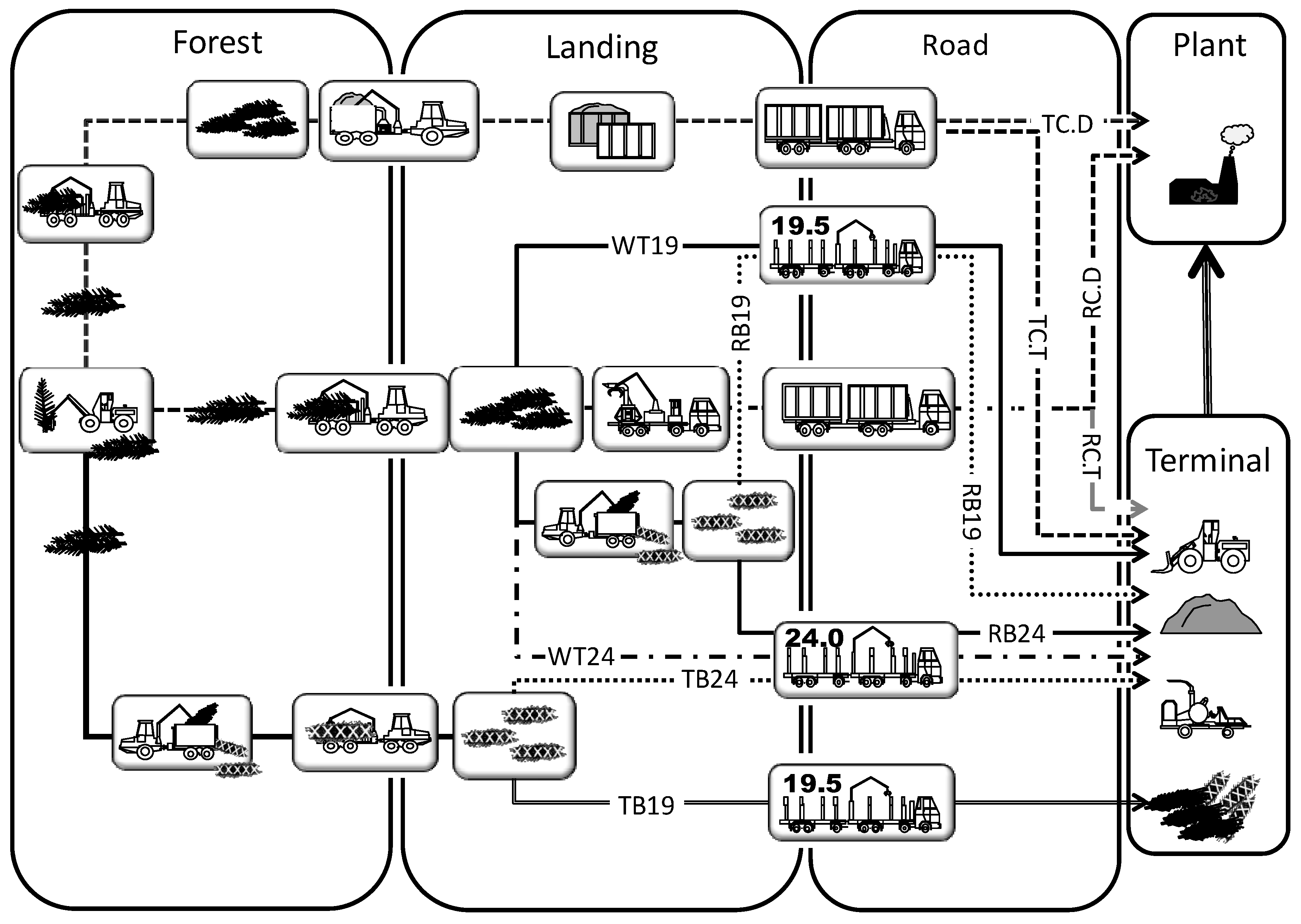
All supply chains were initiated with mechanized felling (Table 2). Terrain transport (extraction) of loose or bundled trees was carried out with a forwarder. In the cases using in-field chipper, the wood material was assumed piled at a suitable location between the cutting site and the roadside. In this particular study it was assumed that this location was 80 m from the roadside. The motive for this solution, which is quite common in Norway, is the lack of suitable landings for energywood piles along the forest road network. Bundling could take place in-field or at roadside, while chipping could take place at an intermediate landing location between the cutting site and the roadside, at roadside landing, or at terminal (Figure 1). The efficiencies of extraction, loading, road transport with two truck configurations, and comminution, as well as material and dry matter losses through storing of different forms of biomass, were modelled. The main energy carriers were whole trees, tree parts, bundles or chips.

Table 2. Abbreviation and description of the 10 supply systems.

Abbrev.	Description of Supply Chain
WT19	Whole Tree transport from roadside to terminal using a 19.5 m timber truck. This chain is characterized by its low requirement on investment and cost effective chipping, but has high transport costs at longer distances
WT24	Essentially the same as WT19, but uses a 24 m timber truck for road transport
TB19	Terrain Bundling (in-field bundling) to reduce extraction and transport costs. Bundles are extracted to the roadside for drying, then on to the terminal for storage and finally chipping. Road transport with 19.5 m timber truck
TB24	Same as for TB19, but using a 24 m timber truck
RB19	Roadside Bundling. Whole trees are bundled at roadside before transport to the terminal. This implies lower bundling costs than for the TB chains (as the material is concentrated, and the bundler is truck mounted and not forwarder mounted—which is cheaper and more mobile.). This chain has a higher terrain transport (extraction) cost than those with bundling in the field. Road transport to terminal with 19.5 m timber trucks
RB24	Same as for RB19, but with 24 m timber trucks
RC.T	Roadside Chipping and on to Terminal. The material is chipped into containers at the roadside landing. Transported with container truck to terminal, and on to conversion plant with chip truck
TC.T	Terrain Chipping (the pile is located in the terrain) to Terminal. Same as for RC.T, but the material to be chipped is piled (by forwarder) at a suitable landing between the cut area and the forest road. Chipping is done with a forwarder mounted chipper having a chip bin for extraction to containers on the roadside. This is a commonly used method in areas where it is difficult to find suitable roadside landings—i.e., with limited space (e.g., near larger public roads, in steep areas, or because of pour drying conditions on the roadside)
RC.D	Roadside Chipping, Direct delivery to conversion plant. The material is chipped into containers at the roadside landing, and is transported by container truck directly to the conversion point. This chain has lower storage costs and shorter total transport distance (no transport to buffer) than RC.T, but is a ‘hot’ system requiring more intensive management, it has no buffer, and is more weather dependent than the others. Probably the most common method of production of chips from harvesting residues overall.
TC.D	Terrain Chipping (the pile is located in the terrain), Direct delivery to final conversion plant. Same as TC.T except that the material is transported directly to the conversion plant.

Table 2. Abbreviation and description of the 10 supply systems.

Abbrev.	Description of Supply Chain
WT19	Whole Tree transport from roadside to terminal using a 19.5 m timber truck. This chain is characterized by its low requirement on investment and cost effective chipping, but has high transport costs at longer distances
WT24	Essentially the same as WT19, but uses a 24 m timber truck for road transport
TB19	Terrain Bundling (in-field bundling) to reduce extraction and transport costs. Bundles are extracted to the roadside for drying, then on to the terminal for storage and finally chipping. Road transport with 19.5 m timber truck
TB24	Same as for TB19, but using a 24 m timber truck
RB19	Roadside Bundling. Whole trees are bundled at roadside before transport to the terminal. This implies lower bundling costs than for the TB chains (as the material is concentrated, and the bundler is truck mounted and not forwarder mounted—which is cheaper and more mobile.). This chain has a higher terrain transport (extraction) cost than those with bundling in the field. Road transport to terminal with 19.5 m timber trucks
RB24	Same as for RB19, but with 24 m timber trucks
RC.T	Roadside Chipping and on to Terminal. The material is chipped into containers at the roadside landing. Transported with container truck to terminal, and on to conversion plant with chip truck
TC.T	Terrain Chipping (the pile is located in the terrain) to Terminal. Same as for RC.T, but the material to be chipped is piled (by forwarder) at a suitable landing between the cut area and the forest road. Chipping is done with a forwarder mounted chipper having a chip bin for extraction to containers on the roadside. This is a commonly used method in areas where it is difficult to find suitable roadside landings—i.e., with limited space (e.g., near larger public roads, in steep areas, or because of pour drying conditions on the roadside)
RC.D	Roadside Chipping, Direct delivery to conversion plant. The material is chipped into containers at the roadside landing, and is transported by container truck directly to the conversion point. This chain has lower storage costs and shorter total transport distance (no transport to buffer) than RC.T, but is a ‘hot’ system requiring more intensive management, it has no buffer, and is more weather dependent than the others. Probably the most common method of production of chips from harvesting residues overall.
TC.D	Terrain Chipping (the pile is located in the terrain), Direct delivery to final conversion plant. Same as TC.T except that the material is transported directly to the conversion plant.

Figure 1. Graphic representation showing the individual pathways of the 10 supply chains.

Figure 1. Graphic representation showing the individual pathways of the 10 supply chains.

2.1. Stand Information

All the trees were assumed felled with a harvester base machine equipped with a multi-tree harvesting head [31], and all the material destined for energy only. The volume available at each stand was generated from a gamma function with a lower limit of 30 m³_s and 95% varying between 60–235 m³_s (Figure 2). The mean object volume removed was 130 m³_s. The individual trees had a mean stem volume of 40 litres (50 litres including top and branches). A mixed stand of lighter (spruce, pine, alder and poplar) and heavier (birch, rowan) species and tree parts (branches) was used assuming a mean basic density (BD) of 400 kg_d m⁻³_s and an initial moisture content of 50%.

Figure 2. The gamma distribution used in generating object volumes.

Figure 2. The gamma distribution used in generating object volumes.

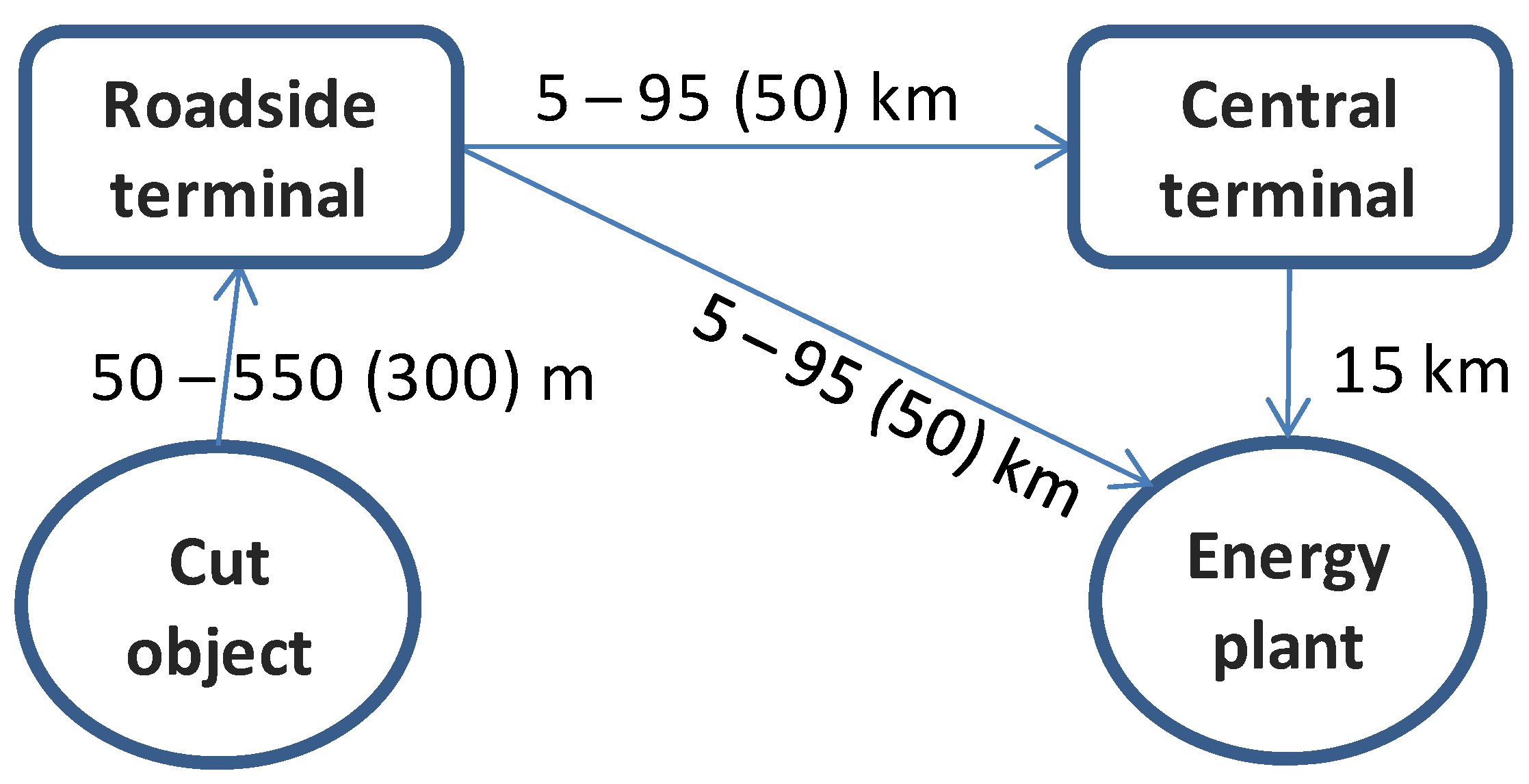
2.2. Spatial Aspects of the Supply Chain

A basic supply chain model was constructed to represent the majority of possible scenarios. It was initiated in the forest stand, included a landing at the forest road, a district terminal, and ended at the energy conversion plant (Figure 3). Transition through the terminal was optional, as per the description of the chains in Table 2. Extraction distances in terrain and on road were set using uniform distributions with ranges and means according to Figure 3. The extraction distance between the harvest site and the roadside landing ranged between 50–550 m, with a mean of 300 m. The distances between the roadside landing and the central terminal were in the range 5–95 km (mean 50 km) and between the terminal and the conversion plant it was fixed at 15 km. The direct distance between the landing and the conversion plant was also 5–95 km with a mean of 50 km.

Figure 3. A schematic diagram of the constructed supply chain.

Figure 3. A schematic diagram of the constructed supply chain.

2.3. Time Consumption and Unit Costs Used in the Model

Machine ownership and utilization costs (Table 3) were calculated using the spreadsheet model for calculation of forest operations costs developed by the European Cooperation in Science and Technology (COST) program’s Action FP0902 (Development and Harmonisation of New Operational Research and Assessment Procedures for Sustainable Forest Biomass Supply) [32,33]. Purchase costs for the different machines were set based on advertisements for similar equipment found on internet based machine exchanges. Fixed costs included depreciation, interest, insurance, garaging and licensing. Depreciation was calculated linearly using a real rate of 5%. Insurance premiums were set at 1% of the purchase price for all machines. The variable costs included fuel and lubricants, maintenance and repair, as well as personnel costs. The price for non-road machine diesel (reduced tariff) was € 1.12 L⁻¹. Personnel costs were based on the agreed tariffs for machine operators [34] and adding mandatory social costs such as pension contributions, employers’ national insurance contributions, vacation pay and insurance—in total a 30% on cost. A 10% overhead, based on the sum of these costs, was charged for personnel administration. The basic salary was € 21.63 per scheduled machine hour (SMh) and the total salary cost was € 33.75 SMh⁻¹. Relocation costs were not included in the machine costing, but were generated for each stand directly according to the later description of each machine. Finally, a company profit margin of 10% was calculated on the basis of the fixed, variable, and personnel costs.

Table 3. Assumptions on characteristics, purchase price, scheduled annual use, machine utilization, expected service life, repair factor and salvage value.

	Power	Mass	Purchase	SMh	MU	Life	Repair	Salvage
Machine	kW	t	€	year−1	%	years	%	value, %
Harvester	170	20	375,000	1,840	75	10 a	100 b	20 a
Forwarder	130	17	275,000	1,840	80	10 a	80 b	25 a
Terrain bundler	136	20	462,500	1,840	71	10 b	80 b	25 b
Roadside bundler	136	17	375,000	1,840	75	10 b	80 b	25 b
Terrain chipper	350	30	625,000	1,040	76	12 b	80 b	25 b
Roadside chipper	350	28	437,500	1,040	74	12 b	80 b	25 b
Terminal chipper	350	25	400,000	1,040	90	12 b	80 b	20 b

^a Spinelli and Magagnotti [35], ^b Lyons, Ackerman, Belbo, Eliasson and Jong [32]; note: Repair denotes the expected repair and maintenance costs through the economic life of the machine.

Table 3. Assumptions on characteristics, purchase price, scheduled annual use, machine utilization, expected service life, repair factor and salvage value.

	Power	Mass	Purchase	SMh	MU	Life	Repair	Salvage
Machine	kW	t	€	year−1	%	years	%	value, %
Harvester	170	20	375,000	1,840	75	10 a	100 b	20 a
Forwarder	130	17	275,000	1,840	80	10 a	80 b	25 a
Terrain bundler	136	20	462,500	1,840	71	10 b	80 b	25 b
Roadside bundler	136	17	375,000	1,840	75	10 b	80 b	25 b
Terrain chipper	350	30	625,000	1,040	76	12 b	80 b	25 b
Roadside chipper	350	28	437,500	1,040	74	12 b	80 b	25 b
Terminal chipper	350	25	400,000	1,040	90	12 b	80 b	20 b

^a Spinelli and Magagnotti [35], ^b Lyons, Ackerman, Belbo, Eliasson and Jong [32]; note: Repair denotes the expected repair and maintenance costs through the economic life of the machine.

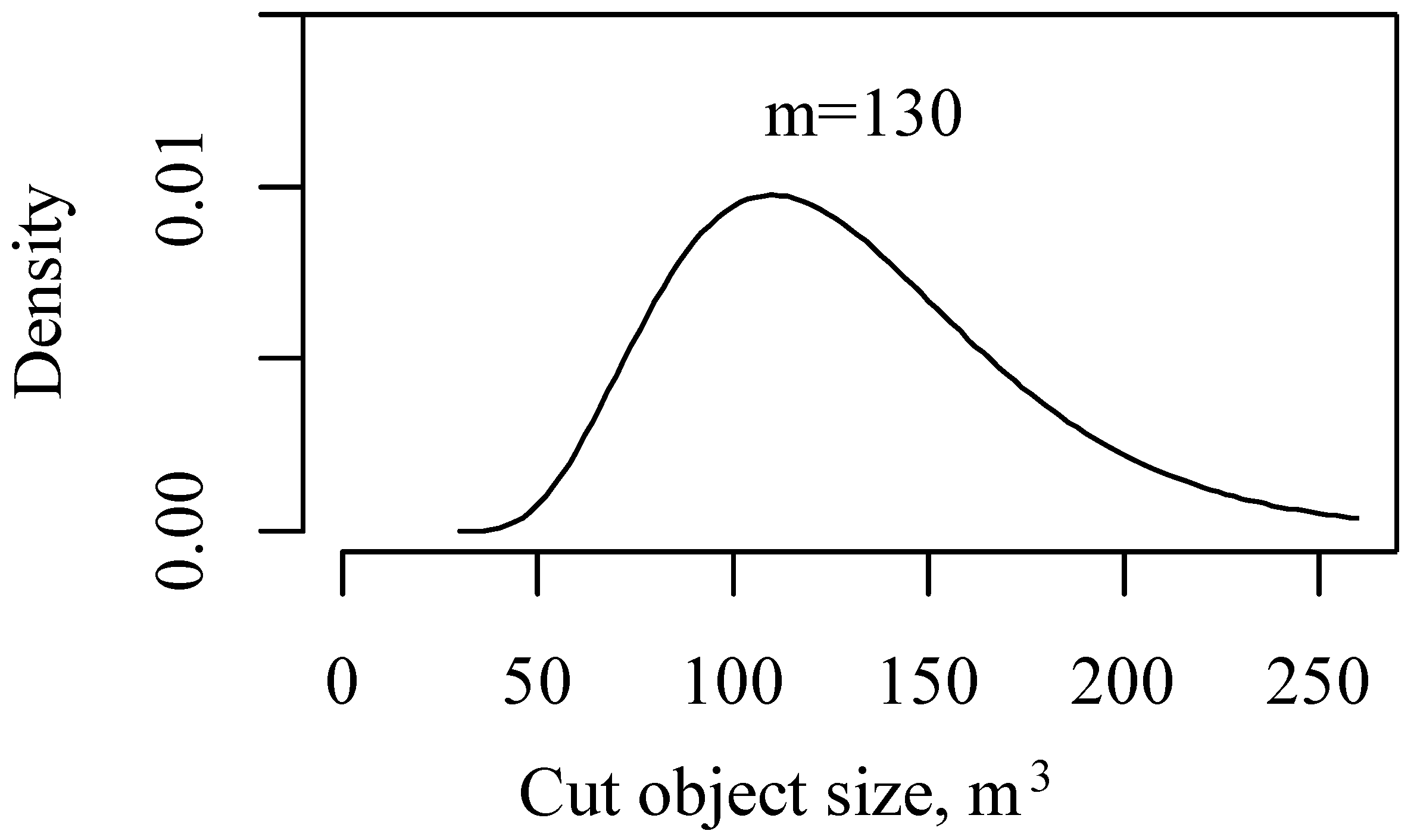
Productivity models for each operation were found or deduced from relevant performance studies published in journals and work reports. The original models were converted to provide productivity, or time consumption, per dry tonne of biomass.

2.4. Harvesting

Harvesting was carried out with a conventional harvester (~170 kW, 20 t). Machine characteristics and cost estimates are shown in Table 3 and Table 4. Diesel consumption was set at 0.095 L kW⁻¹ PMh⁻¹₁₅ and expenses for oil and lubricants was set at 12.6% of the fuel costs for the harvester [36]. The operator was reimbursed for 50 km of personal transport per day. An additional charge of € 3.5 PMh₁₅⁻¹ was levied for saw chain and guide bars. The mean productivity for such an operation harvesting small whole trees for energy was calibrated from other studies [31,37] and assumed to be around 10.5 m³_s PMh₁₅⁻¹. In addition to the estimated hourly cost, a relocation and start-up cost of € 375 is charged per new site to cover machine relocation and administration.

(1)

Table 4. Cost estimates of the machinery and trucks.

Machine Category		Hourly Machine Cost (€ PMh15−1)				Distance Based Cost (€ km−1)	Relocation Cost (€ site−1)
	Fixed	Variable	Operator	Margin	Total
Harvester	34	52	45	13	144	-	375
Forwarder	23	33	42	10	108	-	375
Terrain bundler	42	57	48	15	161	-	375
Roads bundler	34	36	45	11	126	-	375
Terrain chipper	89	108	45	24	266	-	375
Roadside chipper	65	96	46	21	228	-	125
Terminal chipper	49	107	38	19	213	-	12
WT-truck 19.5					65	0.87	10
WT-truck 24					65	0.87	10
Chip bin truck					65	0.87	50

Table 4. Cost estimates of the machinery and trucks.

Machine Category		Hourly Machine Cost (€ PMh15−1)				Distance Based Cost (€ km−1)	Relocation Cost (€ site−1)
	Fixed	Variable	Operator	Margin	Total
Harvester	34	52	45	13	144	-	375
Forwarder	23	33	42	10	108	-	375
Terrain bundler	42	57	48	15	161	-	375
Roads bundler	34	36	45	11	126	-	375
Terrain chipper	89	108	45	24	266	-	375
Roadside chipper	65	96	46	21	228	-	125
Terminal chipper	49	107	38	19	213	-	12
WT-truck 19.5					65	0.87	10
WT-truck 24					65	0.87	10
Chip bin truck					65	0.87	50

2.5. Bundling

Bundling was either done in-field with a bundler mounted on a forwarder chassis (terrain-going bundler) or at roadside with a truck mounted bundler. Machine characteristics and cost estimates are shown in Table 3 and Table 4. Diesel consumption was set at 11 L PMh₁₅⁻¹, and the cost of oil and lubricants was calculated at 8% of the fuel cost. Startup costs (primarily relocation) were set at € 375 per site for the in-field bundler and €125 per site for the truck-mounted bundler. The time consumption for bundling was set at 10 PMmin₁₅ t_d⁻¹ [38] irrespective of the raw materials or whether the bundler operates at the roadside landing or in the terrain. Observations show that bundling at roadside can be time consuming because of the need to handle and stack the bundle after production, while in-field the machine just moves away from the bundle [38]. Also, in-field, the bundling work is ongoing while the forwarder is moving, meaning that it is not very dependent on the movement time. The bundles were assumed to have a mean diameter of 0.7 m, a length of 3.0 m, and a volume of 1.15 m³_b. Bundles were assumed to have a density of 210 kg_d m⁻³_b. The method for calculating bundling costs is given in Equation (2), with the parameters shown in Table 5.

(2)

Table 5. Model parameters for the bundling module.

Parameter	Bundling in Terrain	Bundling at Roadside
Tbundling (PMmin15 td−1)	10	10
h. rate (€ PMh15−1)	156	125
Set up cost, (€ site−1)	375	125

Table 5. Model parameters for the bundling module.

Parameter	Bundling in Terrain	Bundling at Roadside
Tbundling (PMmin15 td−1)	10	10
h. rate (€ PMh15−1)	156	125
Set up cost, (€ site−1)	375	125

2.6. Chipping

The different chipping locations (in-field, roadside landing, or terminal) place differing demands on the properties of the chipper. A chipper permanently located at a terminal or conversion plant requires almost no mobility and allows the machine to be built onto a rather low-cost chassis. Mobile chippers intended for chipping at various locations are often mounted on a truck chassis, and if they are to operate along the forest road network in wet and icy conditions they need a platform with rather good traction (e.g., four drive wheels on truck). In-field chippers are usually mounted on forwarders, with a separate power unit for the chipper, and a bin 15–20 m³_l for transporting the chips to roadside (Table 6). Talbot and Suadicani have demonstrated the relation between terrain transport distance, chip bin size and chipping productivity towards the cost-efficiency of a two-machine system with an in-field chipper and a bin forwarder [19]. In the present case, with 80 m transport distance and a relatively large chip bin on the forwarder mounted chipper, these two options were considered to have near equal economic performance and the single machine system was chosen. Because most Norwegian terminals still handle relatively small volumes annually, a truck-mounted chipper was chosen also for chipping at terminal in this study. For terminals (or conversion plants) having a large annual throughput, a dedicated stationary chipper could provide a more cost-efficient chipping option for the supply chains based on road transport of whole trees and bundles.

Table 6. Details of chipper location and configuration.

Location	Base Machine and Chipper
Terminal	6 × 2 wd truck, 350 kW drum chipper
Roadside terminal	6 × 4 wd truck, 350 kW drum chipper
In-field	17 t, 140 kW forwarder, drum chipper with own 350 kW engine and 21 m3l container

Table 6. Details of chipper location and configuration.

Location	Base Machine and Chipper
Terminal	6 × 2 wd truck, 350 kW drum chipper
Roadside terminal	6 × 4 wd truck, 350 kW drum chipper
In-field	17 t, 140 kW forwarder, drum chipper with own 350 kW engine and 21 m3l container

Because of the seasonality of fuel chip demand, chippers were assumed to have a lower degree of utilization in terms of scheduled machine hours per year (Table 3) and their economic lifetime was therefore set at 12 years, with a residual value of 20% of purchase price.

Effective time consumption for chipping was estimated using an Italian time consumption model [39,40] for a self-propelled terminal chipper (Equation (3)). Chipping costs were estimated by time consumption and hourly rate, adding start-up cost per cut object (Equation (4)).

(3)

(4)

where: PS denotes piece size (mean size of the chipped trees or tree parts (t_d)), P is the nominal power (kW) of the engine driving the chipper.

Chipper type, knife wear, screen settings, and wood characteristics all influence the specific fuel consumption during chipping, but this was set at 3.2 L t_d⁻¹, in accordance with the findings of [41]. Additional fuel consumption was estimated for the in-field chipper to cover chip transport from the wood pile located in the terrain to roadside terminal. Oil and lubricant costs were set at 6% of the fuel costs for chippers.

For chipping piles located in the terrain an extraction distance of 80 m to the roadside is assumed, using the same speed as a normal forwarder (38 m·min⁻¹) and 5 min for emptying the bin into the container at roadside. A utilization rate of 76% is assumed for the in-field chipper [42]. For chipping at roadside, delays due to waiting for containers and the more restricted work space decrease the chipper utilization to around 74% [42]. A chipper placed at a central terminal inevitably has good working conditions and a good supply of raw material, and the utilization is set to 90%. The start-up cost for the in-field chipper is the same as for the harvester, in-field bundler and the forwarder, as it also has to be moved with a low-bed truck. The truck-mounted chipper moves under own power, and the much reduced rate for chipping at the terminal is due to the fact that biomass from many stands is combined. Model parameters for the chipping module are given in Table 7.

Table 7. Model parameters for the chipping module.

Parameter	Terrain Pile	Roadside Pile		Terminal Pile
	WT †	WT	Bundles	WT	Bundles
Power (kW)	350	350		350
PMh0/PMh15 *	1	1	1	1	1
Piece volume td	0.015	0.015	0.24	0.015	0.24
Start-up cost (€ site−1)	375	125		12.5

* With chipping studies there is no tradition for separating PMh₀ og PMh₁₅, MU is therefore equal to the ratio between PMh₀ og TMh; ^† Whole Trees.

Table 7. Model parameters for the chipping module.

Parameter	Terrain Pile	Roadside Pile		Terminal Pile
	WT †	WT	Bundles	WT	Bundles
Power (kW)	350	350		350
PMh0/PMh15 *	1	1	1	1	1
Piece volume td	0.015	0.015	0.24	0.015	0.24
Start-up cost (€ site−1)	375	125		12.5

* With chipping studies there is no tradition for separating PMh₀ og PMh₁₅, MU is therefore equal to the ratio between PMh₀ og TMh; ^† Whole Trees.

2.7. Terrain and Road Transport—General Approach

For forwarder extraction, costs are based on time consumption only, while for road trucks, it is common to separate the cost to a time based and a distance based cost [43]. The payload is restricted by limitations on the Gross Vehicle Weight (GVW) or the load space, depending on the density of the material, and is estimated by Equation (5):

(5)

Time consumption per transported unit (t_d) is estimated from Equation (6).

(6)

where: T_{term pd} is the terminal time per dispatched load, i.e., waiting, load-securing, load measuring, record keeping and similar T_{term pt} is terminal time that is related to load size, primarily loading and unloading.

Start-up costs are administration and possible relocation costs related to each cut object. Transport costs are estimated according to Equation (7):

(7)

Parameters used in the transport related equations (Equations 5–7) for the different transport units and supply chain alternatives are found in Table 4, Table 8 and Table 10. The truckload material density is dependent on the solid volume on the load and the basic density of the wood species being transported. With a solid volume content (SVC) of 20% and a BD of 400 kg m⁻³_s, the dry matter density is 80 kg_d m⁻³_l. For the transport of bundles, [27] indicated a SVC on load of 35%, which gives a dry matter density of 140 kg_d m⁻³_l for material having similar BD. Table 4 and Table 8 provides an overview of cost estimates, load capacities, SVC and time consumption estimates used in this study for each transport mode.

Table 8. Parameters for extraction and transport of whole trees (WT), bundles and chips.

	Forwarder WT	Forwarder Bundles	Truck WT 19.5 and (24) m	Truck Bundles 19.5 and (24) m	Truck Chips from Landing (Terminal)
Max load, t	13	13	24.1 (36)	24.1 (36)	29
Max vol, m3l	36	36	91 (120)	91 (120)	85
SVC	0.20	0.35	0.20	0.35	0.4
Tterm pd, PMmin0 truckload−1	0	0	25	25	38 (29)
Tterm pt, PMmin0 m−1s	2.77	2.17	1.4	1.3	0
Mean speed, km h−1	2.3	2.3	12.7 × ln(D) + 9.3
PMh0 PMh15−1	0.92	0.92	1	1	1

Table 8. Parameters for extraction and transport of whole trees (WT), bundles and chips.

	Forwarder WT	Forwarder Bundles	Truck WT 19.5 and (24) m	Truck Bundles 19.5 and (24) m	Truck Chips from Landing (Terminal)
Max load, t	13	13	24.1 (36)	24.1 (36)	29
Max vol, m3l	36	36	91 (120)	91 (120)	85
SVC	0.20	0.35	0.20	0.35	0.4
Tterm pd, PMmin0 truckload−1	0	0	25	25	38 (29)
Tterm pt, PMmin0 m−1s	2.77	2.17	1.4	1.3	0
Mean speed, km h−1	2.3	2.3	12.7 × ln(D) + 9.3
PMh0 PMh15−1	0.92	0.92	1	1	1

2.8. Terrain Transport

Extraction of bundles and uncompressed material was carried out with a conventional forwarder. A typical medium sized forwarder (JD 1210E, Komatsu 860.4, Gremo 1350VT, Ponsse Elk) has a net mass of 16–17 tonnes, a 13–14 tonne payload, 4–5 m² load cross space, and 4.5 m (standard) to 5.5 m (some models) load bed length. The 5.5 m load bed allows for 2 stacks of 3 m bundles to be loaded in tandem. With the shorter load bed, operators load both parallel and perpendicular to the load bed orientation in maximizing the payload. Whole trees of 6 m length can easily be transported on either load bed. Stacking typically exceeds the stanchion height, increasing the load space by 1–2 m². In this study a load space volume of 36 m³_l was assumed for both the transport of bundles and uncompressed whole trees.

Machine characteristics and cost estimates are shown in Table 3 and Table 4. Diesel consumption was set at 0.098 L kW⁻¹ PMh₁₅⁻¹and expenses for oil and lubricants were set at 8% of the fuel costs [36]. The mean travel speed for the forwarder was set to 2.3 km h⁻¹ (38.3 m·min⁻¹) [18]. The time consumption model was based on the results of Laitila et al. [18], where extraction of whole trees with a 10.4 t forwarder (Timberjack 810B) was studied. Time consumption was dependent on the volume per grapple (loading and unloading), and the concentration of material (m³_s 100 m⁻¹ strip-road). For handling of loose trees the grapple volume was set to 0.25 and 0.6 m³_s during loading and unloading respectively, while the corresponding grapple volumes for bundles were set to 0.35 and 0.75 m³_s for loading and unloading. The model from [18] is not considered valid for larger grapple volumes. For both forms of biomass, a concentration of 10 m³_s per 100 m striproad was assumed. This results in a time consumption of 1.60, 0.47 and 0.70 PMmin₀ m⁻¹_s for loading, extracting and unloading loose material. The corresponding values for the case of bundles are 1.08, 0.47 and 0.62 PMmin₀ m⁻³_s. Summed up, this gives a terminal time of 2.77 PMmin₀ m⁻³_s for handling of loose material and 2.17 PMmin₀ m⁻³_s for handling bundles. The ratio of PMh₀ and PMh₁₅ was set to 0.92 and the machine utilization rate (MU) to 0.82 [44].

2.9. Road Transport

In 2010 time and distance based rates for road transport with a conventional timber truck were € 64 h⁻¹ and € 0.7 km⁻¹ [43], which gives an hourly cost of € 99 h⁻¹ at a mean speed of 50 km h⁻¹. Because of increased fuel prices and the costs of having to make some adaptations to the truck to transport whole trees these numbers were estimated to be € 65 PMh₁₅⁻¹ and € 0.88 km⁻¹. In addition to this, a charge of € 62.5 is levied to cover administrative costs with every new site (Table 4).

In the basic scenario, loose material and bundles are transported with a 19.5 m timber truck fitted with a crane and steel plates on the sides and bottom for traffic safety. The maximum allowed mass (gross vehicle weight (GVW)) of such trucks is 50 t. A truck and crane weighs 16.5 t, the trailer 6.5 t, and the steel plates 3 t [38]. The maximal payload is therefore 24.1 t. The dimensions of the load bed are 6.3 m in length, 2.3 m in width and 2.4 m in height, giving a gross load volume of 34.5 m³_l. Comparative dimensions for the trailer load volume are 8.3 m, 2.3 m, and 3 m in length, width, and height, giving a load volume of 56.5 m³_l. The combined load volume is therefore 91 m³_l. The mean travelling speed increases asymptotically with increasing transport distance on public road as against forest road [27].

Timber transport trucks enjoy a special concession on GVW (60 t as against 50 t) and a total length of 24 m [45]. In this study, they are modified in the same way as the 19.5 m trucks, with steel plates for the transport of bundles and whole trees although this is not yet permitted by law which states that this special concession is explicitly for roundwood transport [45].

According to Laitila & Väätäinen [17], T_{term pt} and T_{term pd} for whole tree transport is 1.4 PMmin m⁻³_s and 24 PMmin truckload⁻¹ respectively. For bundles the corresponding values were set at 1.3 PMmin₀ m⁻³_s and 25 PMmin₀ truckload⁻¹ [46].

All chip transport is done with a container truck and trailer, with a hydraulic hook arm. This gives the option of either having a depot of containers at the landing, or chipping directly into the truck. This is a “hot” system, where any delays or disturbances on one part will have repercussions for others. If the truck inter-arrival time is too long, the chipper or chip shuttle comes to a stop, while if the chipper and shuttle are too slow, the interference time is transferred to the trucks [19]. This can reduce the machine utilization rate amongst actors.

The trailer has a tipping capability, which means that the containers do not have to be cross-loaded to the truck for tipping. The containers used in the truck set in this study have a space volume of 38 m³_l and 44 m³_l on the truck and trailer respectively. Normal practice is to slightly overfill the containers as the load settles due to vibration—this increases the load by roughly 3 m³_l. Maximum GVW is 50 t for the truck and trailer, the tare weight for the truck and container is 16 t, while the tare weight for the trailer with container is 7.5 t. The maximum payload and volume is therefore 29 t and 85 m³_l for the truck and trailer. The solid volume content of chips is set to 40% of the space volume [27]. The time and distance related cost components are the same as for the timber transport above.

Time consumption for the placement and loading of containers from the landing was set at 2 and 7 PMmin₀ per container—this includes the placement of the first set of containers at a new stand. The time consumption for unloading at the plant or terminal was set at 10 PMmin₀ per container, including weighing the load and taking samples for moisture assessment [47]. Terminal time T_{term pd} therefore sums to 38 PMmin₀.

At the terminal, chips were loaded with a wheeled front-end loader, and the terminal time for loading was effectively halved. T_{term pd} was therefore calculated as 29 PMmin₀ per load. Time consumption and costs for a wheeled loader were accrued to the total terminal costs.

2.10. Storage and Terminal Costs

Dry matter loss (rot, waste), space costs (paved area, roofing where applicable), and handling costs of material (loading trucks, weighing, moisture content measurements, paper covering etc.) constitute the majority of storage costs. The cost of lost dry matter is calculated as the cost of the biomass equivalent supplied up to that point in the chain, according to Equation (8):

(8)

where: C_{loss i} is the cost of the losses at storage i (e.g., at terminal); γ denotes the proportion of waste at storage point i; α denotes decay (fixed proportion per month) at storage point i; m denotes storage time (months) at storage point i; C_n denotes the unit cost of each operation (e.g., harvesting, forwarding) up to storage point i.

Losses through wasteful handling reduce the volume, while rot reduces the basic density of the material. It has not been possible to find studies of dry matter loss with storage of whole trees. Loss parameters are listed in Table 9. Bundles made from harvesting residues have been shown to have a dry matter loss of 1%–3% per month, where fresh residues from spruce show the highest losses while dry spruce residues and pine residues show the lowest [48]. For both loose and bundled whole trees, dry matter loss was assumed to be somewhere between the 0.5% for spruce pulpwood [49] and bundles of harvesting residues, and was therefore set at 1% per month. Material that is chipped in its fresh state (45%–55%) and stored outdoors will have a dry matter loss of 1%–2% per month [49,50], while dry chips lose almost no dry matter under storage [49].

Table 9. Model parameters for losses due to waste and rot in various stages of supply.

Location		Storage Losses γ (%)	Loss to Rot α, % per Month
In-field	Whole trees	1	0.7
	Bundles	0	0.7
Roadside	Whole trees	0.5	0.7
	Bundles	0.2	0.7
	Chips	0.5	1.0
Terminal	Whole trees	0.1	0.7
	Bundles	0.0	0.7
	Chips	0.1	1.0

Table 9. Model parameters for losses due to waste and rot in various stages of supply.

Location		Storage Losses γ (%)	Loss to Rot α, % per Month
In-field	Whole trees	1	0.7
	Bundles	0	0.7
Roadside	Whole trees	0.5	0.7
	Bundles	0.2	0.7
	Chips	0.5	1.0
Terminal	Whole trees	0.1	0.7
	Bundles	0.0	0.7
	Chips	0.1	1.0

There are no published studies that separate losses in volume with losses in basic density due to rot. In this study it was assumed that half of the losses due to rot are accrued to a reduction in basic density while the other half are written to a reduction in volume (Table 9).

The terminal and storage cost is estimated according to Equation (9) and has three components; fixed area costs (e.g., depreciation on the terminal) is based on the number of months in storage, the variable area costs (e.g., paper cover) is calculated for each delivery, and handling costs are other costs that might occur on the storage facility.

(9)

where: C_{area fixed} and C_{area variable} or the fixed and variable costs for the storage area; h is the storage height; SVC and BD denote the solid volume content and the wood basic density; m is the storage duration in months; C_other is other costs relating to the terminal.

The parameters used in Equation 9 are listed in Table 10. The SVC of the material in storage is assumed to be the same as for with transport with either timber truck or container truck (Table 8). With a stack height of 4 m it is possible to store 0.8 m³_s loose material, 1.4 m³ bundled material and 1.6 m³ of chips per m² of storage space. A roll of paper (4 × 250 m) costs € 625 + transport, c. € 0.75 per m² in purchase and roughly € 0.5 m⁻² in dispensing it.

In whole tree and the bundle chains the material is stored for 11–12 months on average at the roadside landing under cover, 0.5 months covered at the terminal, and 1 month as dry chips at the terminal [48]. In the chains that are defined with chip transport from roadside to terminal or conversion plant, the material is stored for 15 months at roadside, under cover before chipping. As the chips are transported from the roadside landing immediately after chipping, no storage cost for chips accrues there. For the chip transport scenarios that go via a terminal (RC.T & TC.T), the dry chips are stored for one month on average before delivery to the plant.

The chip transport chains with delivery directly from the roadside landing to the conversion plant imply that snow clearing would need to be done for a number of stands in the heating season, in order to provide access from the public roads to the landing. The cost for this is written against the quantity of fuel coming from that particular stand. The assumption was that snow clearing was necessary in one third of the cases, and that it took 3 h, and cost € 188 per stand.

Table 10. Storage costs and moisture content for the various assortments (WT, Bundles, Chip) and supply chain alternatives. The given moisture contents are as per the end of the storage period.

Description	In Field		At Roadside			At Terminal
	WT	Bundles	WT	Bundles	Chip	WT	Bundles	Chip Storage
Fixed space cost, € m−2·yr−1	0	0	0	0	0	12.5	12.5	25
Variable space cost, € m−2	0	0	1.25	1.25	0	1.25	1.25	0
Stack height, m	3.5	3.5	3.5	3.5	2.5	4	4	4.5
SVC at storage	0.2	0.35	0.22	0.35	0.4	0.22	0.35	0.4
Storage time (mnths) WT’s;	0.5		11			0.5		1
Moisture content WT’s	50		35			35		35
Storage time (mnths) TB’s	0.4	0.1		11			0.5	1
Moisture content TB’s	50	47		35			35	35
Storage time (mnths) RB’s;	0.5		7	3			0.5	1
Moisture content RB’s	50		40	35			35	35
Storage time (mnths) CH’s,	0.5		15		0.01			1
Moisture content, CH’s	50		35		35			35
Handling in storage, € td−1						3.94	3.94	3.94
Handling in storage, € per tract			62.5			-

Table 10. Storage costs and moisture content for the various assortments (WT, Bundles, Chip) and supply chain alternatives. The given moisture contents are as per the end of the storage period.

Description	In Field		At Roadside			At Terminal
	WT	Bundles	WT	Bundles	Chip	WT	Bundles	Chip Storage
Fixed space cost, € m−2·yr−1	0	0	0	0	0	12.5	12.5	25
Variable space cost, € m−2	0	0	1.25	1.25	0	1.25	1.25	0
Stack height, m	3.5	3.5	3.5	3.5	2.5	4	4	4.5
SVC at storage	0.2	0.35	0.22	0.35	0.4	0.22	0.35	0.4
Storage time (mnths) WT’s;	0.5		11			0.5		1
Moisture content WT’s	50		35			35		35
Storage time (mnths) TB’s	0.4	0.1		11			0.5	1
Moisture content TB’s	50	47		35			35	35
Storage time (mnths) RB’s;	0.5		7	3			0.5	1
Moisture content RB’s	50		40	35			35	35
Storage time (mnths) CH’s,	0.5		15		0.01			1
Moisture content, CH’s	50		35		35			35
Handling in storage, € td−1						3.94	3.94	3.94
Handling in storage, € per tract			62.5			-

3. Results and Discussion

Bundles were the most cost effective product for extraction at € 21 t_d⁻¹, but the cost of in-field bundling, at € 31 t_d⁻¹ made the total cost delivered at roadside (€ 93 t_d⁻¹) marginally more expensive than extracting whole trees and bundling at roadside (€ 92 t_d⁻¹ ,Table 11). Extraction of loose material and roadside chipping (€ 92 t_d⁻¹) was substantially cheaper than in-field chipping and extraction of chips (€ 108 t_d⁻¹).

Table 11. Mean costs and standard deviations for the individual components and overall supply chains (€ t_d⁻¹); because harvesting costs (41 ± 2) were considered invariant to supply chain alternative, this cost component is not shown but is included in the total cost column.

	Forwarding	Bundling	Chipping	Road transport 1	Road transport 2	Losses	Storage	Total
WT19	28 ± 5	0	21 ±	27 ± 11	8	9 ± 1	12 ± 0	146 ± 13
WT24	28 ± 5	0	21 ± 0	21 ±	8	9 ± 1	12 ± 0	139 ± 11
TB19	21 ± 3	31 ± 2	18 ± 0	16 ± 6	8	10 ± 1	11 ± 0	156 ± 9
TB24	21 ± 3	31 ± 2	18 ± 0	12 ± 5	8	10 ± 1	11 ± 0	152 ± 8
RB19	28 ± 5	23 ± 1	18 ± 0	16 ± 6	8	9 ± 1	15 ± 1	158 ± 10
RB24	28 ± 5	23 ± 1	18 ± 0	12 ± 5	8	9 ± 1	15 ± 1	155 ± 9
RC.T	28 ± 5	0	23 ± 2	17 ± 6	8	12 ± 1	9 ± 1	139 ± 11
TC.T	28 ± 5	0	39 ± 2	17 ± 6	8	13 ± 1	9 ± 1	155 ± 11
RC.D	28 ± 5	0	23 ± 2	20 ± 8	0	11 ± 1	6 ± 1	128 ± 12
TC.D	28 ± 5	0	39 ± 2	20 ± 8	0	11 ± 1	6 ± 1	145 ± 12

Table 11. Mean costs and standard deviations for the individual components and overall supply chains (€ t_d⁻¹); because harvesting costs (41 ± 2) were considered invariant to supply chain alternative, this cost component is not shown but is included in the total cost column.

	Forwarding	Bundling	Chipping	Road transport 1	Road transport 2	Losses	Storage	Total
WT19	28 ± 5	0	21 ±	27 ± 11	8	9 ± 1	12 ± 0	146 ± 13
WT24	28 ± 5	0	21 ± 0	21 ±	8	9 ± 1	12 ± 0	139 ± 11
TB19	21 ± 3	31 ± 2	18 ± 0	16 ± 6	8	10 ± 1	11 ± 0	156 ± 9
TB24	21 ± 3	31 ± 2	18 ± 0	12 ± 5	8	10 ± 1	11 ± 0	152 ± 8
RB19	28 ± 5	23 ± 1	18 ± 0	16 ± 6	8	9 ± 1	15 ± 1	158 ± 10
RB24	28 ± 5	23 ± 1	18 ± 0	12 ± 5	8	9 ± 1	15 ± 1	155 ± 9
RC.T	28 ± 5	0	23 ± 2	17 ± 6	8	12 ± 1	9 ± 1	139 ± 11
TC.T	28 ± 5	0	39 ± 2	17 ± 6	8	13 ± 1	9 ± 1	155 ± 11
RC.D	28 ± 5	0	23 ± 2	20 ± 8	0	11 ± 1	6 ± 1	128 ± 12
TC.D	28 ± 5	0	39 ± 2	20 ± 8	0	11 ± 1	6 ± 1	145 ± 12

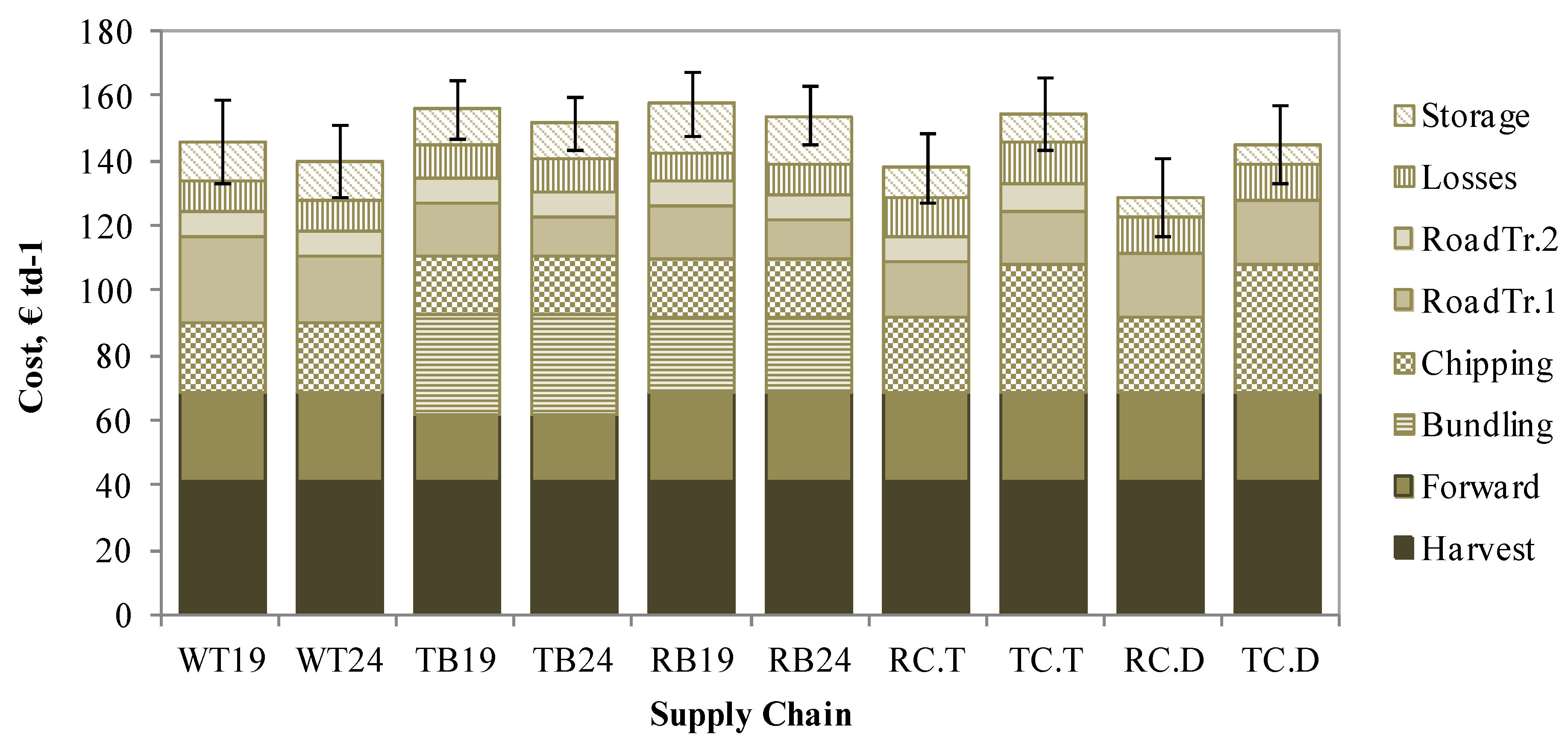
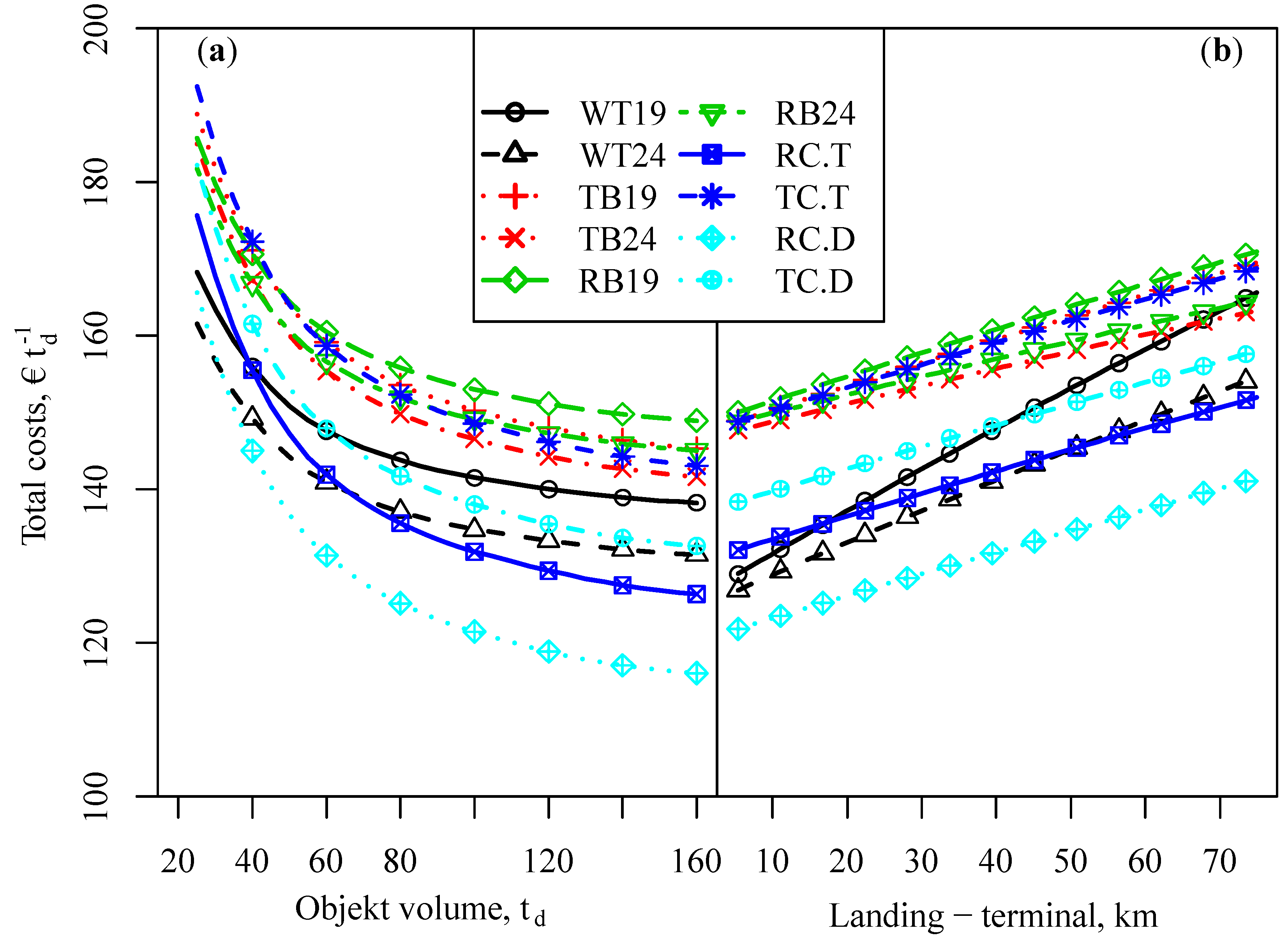
The whole tree chains (WT19 and WT24) showed costs of € 146 t_d⁻¹ and € 139 t_d⁻¹ delivered to plant respectively, despite having excessively high road transport costs, especially on the conventional 19.5 m trucks. For the whole-tree chains, chipping costs were around 14% higher than for bundle chains, and 23% lower than for chip transport chains with their decentralized chipping. For whole tree and bundle chains (WT, TB, RB), use of the 24 m timber truck provides a saving of ca. 12% for road transport and ca. 2% over the whole supply chain, as compared to the use of the standard 19.5 m truck. Chip transport from roadside landing is 23% cheaper than whole tree transport with the 24.0 m truck, and 59% cheaper than the 19.5 m truck. Re-directing chips via the terminal (RC.T, TC.T) results in an extra cost of € 11 t_d⁻¹ (7%–9%) as against direct delivery. Overall, there is a difference of just under € 30 t_d⁻¹ (10%) between the cheapest (RC.D—roadside chipping with direct delivery) and most expensive (RB19—roadside bundling and transport via terminal) supply chains. Roadside chipping, whether transported directly to the plant or via the terminal, is consistently cheaper than any other supply chain configuration.

Figure 4 provides a graphic overview of the same data as Table 11, including the standard deviation around the total supply performance.

Chip transport from the roadside landing via the terminal (RC.T) is always more expensive than direct delivery of chips from the same source (RC.D), but this effect can become more or less pronounced, depending on the location of the terminal in relation to the harvesting site and plant (Figure 5). Bundling (TB, RB) results in higher overall costs than all the other supply chains studied, irrespective of object volume or road transport distance. For small stands and short transport distances, whole tree chains are cost effective, as they have lower start-up costs, both with regards to machines in the field, and at the roadside landing.

Figure 4. Delivered cost of chips (€ t_d⁻¹) by supply chain and supply chain component.

Figure 4. Delivered cost of chips (€ t_d⁻¹) by supply chain and supply chain component.

Figure 5. The relationship between total supply cost and object volume (a) and total supply cost and the transport distance between the roadside landing and terminal or final conversion plant (b) for each supply chain scenario.

Figure 5. The relationship between total supply cost and object volume (a) and total supply cost and the transport distance between the roadside landing and terminal or final conversion plant (b) for each supply chain scenario.

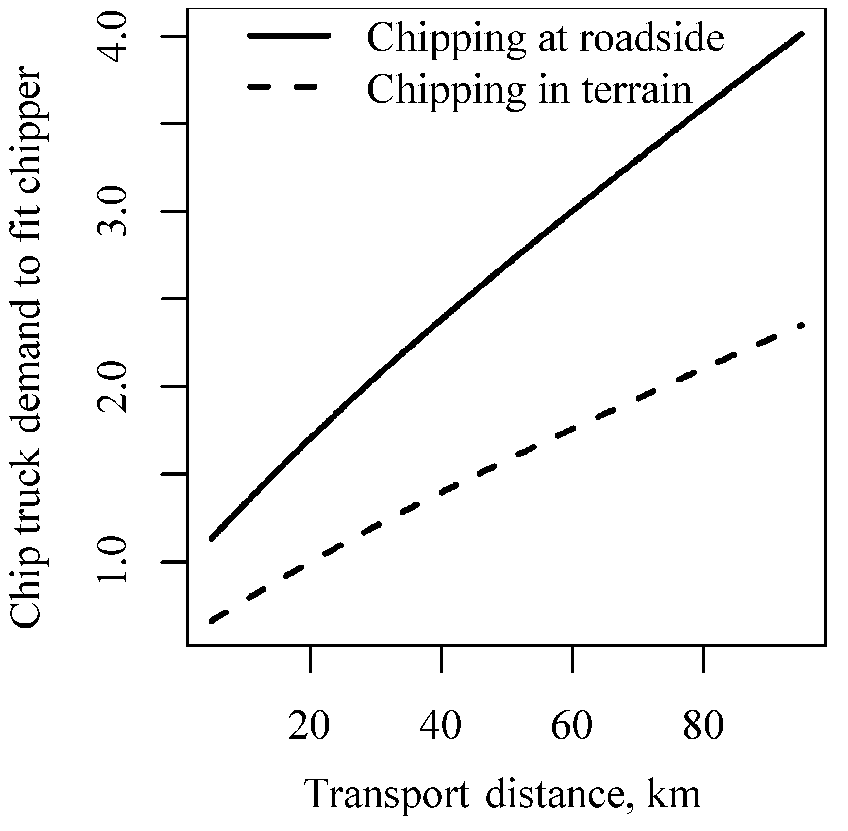
In considering the balance in productivity between the transport component for container trucks and the chipping component at different road transport distances, Figure 6 indicates the ratio between chipper productivity and transport productivity. It can be seen how at e.g., 20 km, in-field chipper productivity is roughly equal to road transport productivity with a single truck, while two trucks are only fully utilized at transport distances approaching 80 km. For chipping at roadside, the corresponding ratios are approximately 1.7 at 20 km, 2.4 trucks at 40 km and 3.7 at 80 km.

Figure 6. Chip truck demand in fitting chip production rates for roadside and in-terrain chipping respectively.

Figure 6. Chip truck demand in fitting chip production rates for roadside and in-terrain chipping respectively.

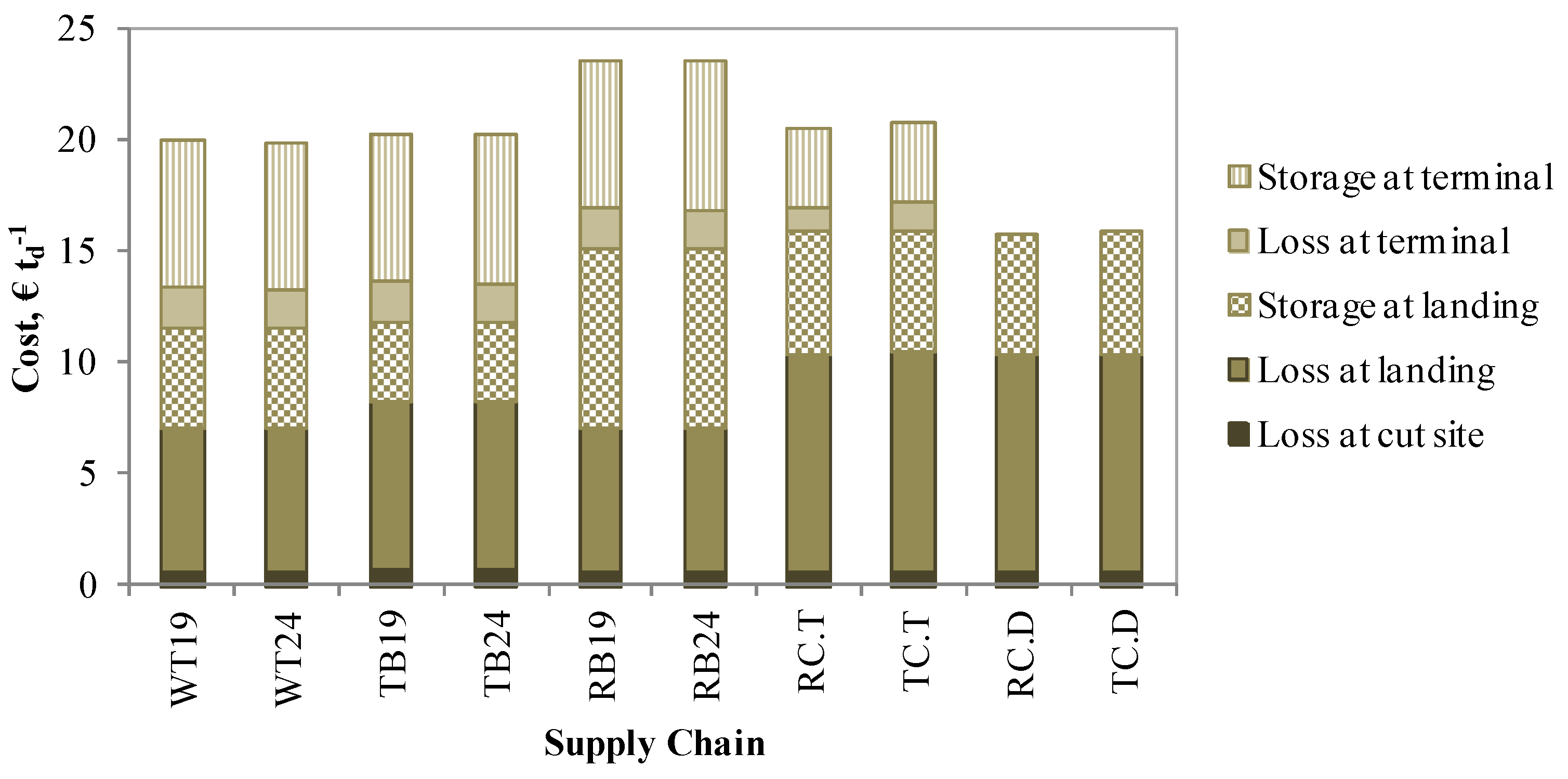
Figure 7 highlights the costs of losses related to storage for the various chains. These costs constitute roughly 10% of the costs of the whole supply chains. The chains that include bundling of material that has been extracted to the roadside landing (RB19 and RB24) show somewhat higher losses and storage costs than in the other chains. This is primarily due to the need to cover the material 2–3 times throughout the chain, twice at the landing (after extraction, and again after bundling), and once at the terminal. The chains with direct deliveries of chips from landing to plant (RC.D and TC.D) show the lowest losses, as expected. The differences between the other chains are not substantial.

Figure 7. Cost of losses for each stage in the supply chain, including in-stand, at landing, and at the terminal.

Figure 7. Cost of losses for each stage in the supply chain, including in-stand, at landing, and at the terminal.

As things stand today, costs in the bundling chains are too high to make these chains competitive with the transport of loose material and chipping/transport from the roadside landing. This is due to the high cost of actual bundling, but also somewhat related to the way the other chains are configured in the study. A large number of suppliers in Norway use long term storage and drying at the terminal before chipping. For this production chain, it would be of more benefit to have a space effective and stable assortment than for chains where the storage primarily takes place at the roadside landing.

The transport of chips directly from roadside landing to the final conversion plant is a cost effective alternative, especially with larger object volumes and longer distances. This supports the findings of Laitila [51]. However, it is a pre-requirement that this hot system is well coordinated and that delays and interference on production or transport do not arise.

The transport of whole trees with timber truck was effective for small stands and short transport distances, while performance was average in the other situations. This chain benefits from the advantages of centralized chipping—especially with small object volumes, as the start-up costs of the chipper are avoided. Two other advantages of this system, which are only partly emphasized in the model, are the fact it utilizes existing capacity and material as per the transport of roundwood, and that like the case for bundles, it is a cold system, where supply chain entities have no dependence on each other. The first point implies both a lower level of specific capital investment in the chain, and that all production areas are well covered by the necessary technology. The fact that it is a cold system implies much reduced demand on planning input and technology, and almost no potential interference between actors.

It is common to utilize more stationary chippers at larger terminals, often trailer-based or tracked machines. These are usually fed by the truck driver directly during off-loading, which further reduces the chipping costs, often down to approximately 50% of those at the roadside landing [52]. In the cases where annual volumes being processed at the terminal justify such a chipper, the chains using whole-tree or bundle transport (WT, TB, RB) will be substantially more cost-efficient than shown in our results. If the chipping costs of these supply alternatives were halved, it would imply a cost reduction of about 10 € t_d as compared to our results. The break even points between e.g., WT24 and RC.D (Figure 5) would be skewed substantially towards larger object sizes and longer transport distances.

Chip terminals have been shown not to be profitable supply chain modules in their own right, but are considered necessary by many managers in guaranteeing supply contracts. The terms and conditions of such contracts vary and the consequences have not been evaluated in this paper. Terminals do offer an opportunity to blend, sort, upgrade, allocate, and cross load biofuels according to various customer’s requirements. This potential has not been demonstrated by research. However, it has been possible to quantify the cost of owning, maintaining and operating terminals.

4. Conclusions

The results of the present study are considered to give a good indication of how the individual chains respond to various factors, and which chains come to the fore under which conditions. The small overall standard deviations (6%–9% of mean costs) show that the results can be interpreted as robust outcomes of high likelihood, extendable in similar forest conditions. The components in this model are somewhat simplified in order to accommodate a broad range of alternatives. According to the results obtained in this study, roadside chipping with direct transport to the plant was consistently the most economically viable method of supplying biomass from small tree harvesting. Roadside bundling and transport of bundles was the most expensive production method in all scenarios. As object quantities increased beyond 60 dry tonnes, the roadside chipping via terminal chain out-competed whole tree transport with a 24 m truck. The direct delivery of material chipped at roadside offered the cheapest transport cost, while whole-tree transport was most sensitive to transport distance. The cost of losses to various causes were modelled and shown to be substantial, yet greatest in the bundling chains.

Even though the results of the present study are considered consistent and indicative of how various factors affect the economic performance and ranking of the different supply chain alternatives, it is important to keep in mind how our system selection, modelling approach and local conditions affect the results. Among the more obvious issues, one could mention that if the national legislation concerning maximum size of truck and trailer combinations equalized timber trucks and chip trucks, the supply chain alternatives based on road transport of chips would increase their competitive advantage of higher biomass density during transport. The potential savings and the impact to the presented results of a dedicated stationary terminal chipper have already been discussed. A successful development and implementation of an integrated feller-bundler system like the “Fixteri” [20,21] may also improve the economic performance of the bundle system.