Article

The Role of Wood Density Variation and Biomass Allocation in Accurate Forest Carbon Stock Estimation of European Beech (Fagus sylvatica L.) Mountain Forests

1
National Institute for Research and Development in Forestry “Marin Drăcea”, 128 Eroilor Boulevard, 077190 Voluntari, Romania
2
Faculty of Silviculture and Forest Engineering, “Transilvania” University of Brașov, Șirul Beethoven 1, 500123 Brașov, Romania
*
Author to whom correspondence should be addressed.
Forests 2024, 15(3), 404; https://doi.org/10.3390/f15030404
Submission received: 23 January 2024 / Revised: 16 February 2024 / Accepted: 18 February 2024 / Published: 20 February 2024
(This article belongs to the Special Issue Biomass Estimation and Carbon Stocks in Forest Ecosystems—Volume II)

Abstract

:
The European beech (Fagus sylvatica L.) is one of the most common tree species in Romania, with importance both economically and environmentally. Accurate methods of biomass assessment at the tree compartment level (i.e., stump, stem, branches, and leaves) are necessary for carbon stock estimation. Wood density (WD) is an important factor in determining biomass and, ultimately, the tree’s carbon content. The average tree density was found to be 578.6 kg/m3. For this study, WD was evaluated by the weighting method related to tree volume. Also, to investigate a practical approach to determining the weighted wood density (WWDst), models were run using density at the base of the tree (WDBase), density at breast height level using discs (WDDBH), the wood core density (WDic), and the diameter at breast height (DBH) as predictors. The biomass assessment was conducted using different model evaluations for WWDst as well as allometric equations using the destructive method. From the results, it was noted that using the WWDst, the total biomass was underestimated by −0.7% compared to the biomass measured in the field. For allometric equations that included DBH and tree height as independent variables, the explained variability was around 99.3% for total aboveground biomass (AGBtotal), while it was 97.9% for allometric function using just the DBH. Overall, the distribution of biomass across different compartments was as follows: 73.5% in stems, 23.8% in branches, 1.9% in stumps, and 1.3% in leaves. The study findings offer valuable insights into WD, biomass distribution among different components, and biomass allometric quantification in natural beech forest environments in mountainous areas.

1. Introduction

In order to reduce human-induced emissions and move towards a carbon-neutral economy, a particular role is played by the capacity of forests to absorb CO2 and store it as carbon in tree biomass. Therefore, accurate estimation of forest carbon stock and change in carbon stock is of significant importance in addressing the challenges posed by climate change. Estimating carbon stock changes in land use management activities, particularly in conversion activities such as deforestation, is of great interest for the forestry sectors as well as for mitigating the impact of climate change [1]. Accurate carbon stock estimation not only helps to assess the impact of these activities (i.e., deforestation) on carbon emissions but also serves as a crucial tool in designing and implementing effective policies aimed at reducing greenhouse gas emissions and promoting carbon sequestration. Also, it can help establish a framework as clearly as possible for upcoming climate scenarios [2]. The Intergovernmental Panel on Climate Change (IPCC) guidelines suggest the use of accurate country- or species-specific wood density (WD) values for high confidence in determining forest biomass and carbon storage [3,4]. Under the United Nations Framework Convention on Climate Change (UNFCCC), reports regarding forest resources and country-specific methods for determining WD [5] are required because they are of great importance for biomass estimation [6] as well as for conversion to carbon stock [7]. Besides country specificity, species-specific traits should also be taken into account as WD is characterized by high variability between tree species [8]. For instance, the shade tolerance characteristic of tree species is reflected in WD, with light-demanding tree species having a more pronounced height growth and presenting a lower density of accumulated matter [9], while shade-tolerant tree species, such as beech, have slower growth with narrower rings and a higher density of wood [10].
The density of wood is the relationship between the mass of a tree and its volume, which are challenging characteristics to measure. One of the non-destructive methods currently used in practice with good results is to calculate the ratio between the mass and volume of an increment core [4,11]. However, depending on which tree stem part is being extracted or the size of the sample (i.e., the core sample), this more convenient method may lead to misleading results that may not be representative of the entire tree bole [12]. Moreover, collecting increment cores from bark to pith is often difficult and can present several challenges, with the main ones as follows: (1) trees have large diameters for the borer to reach the pith; (2) the borer can miss the pith, passing it; and (3) difficulties in inserting the borer, especially in deciduous species [11].
On the other hand, the destructive method (disc extraction along tree stems) requires more time and effort but has high precision in biomass estimation [6,13]. This method was also used in a prior study [14], where WD was considered the second most important predictor after the tree DBH in the evaluation of tree biomass. Classical WD assessment and biomass estimation by destructive methods, which involve felling the tree and collecting discs along the tree stem, have high accuracy but involve complex logistics with high costs and are also time-consuming [15,16]. Although the destructive method limits the estimation of tree densities for species with larger ranges, it can be very useful at the regional level. Studies on average WD by disc method collection along tree stems have been undertaken in different parts of the world, both in managed [16,17,18,19,20] and old-growth forests [21], where an essential zonal knowledge of WD is of real help in subsequent reports on further biomass estimation under UNFCCC. Wood density is often expressed in these studies as oven-dry mass divided by the fresh volume of a representative wood sample [22,23].
The estimation of aboveground biomass (AGB) constitutes an important aspect of carbon stock and global carbon balance in forests [24] as it represents up to 80% of the total tree biomass [3]. Thus, the precise assessment of forest carbon stock relies on the accuracy of AGB estimations. Even though the most accurate and oldest method for estimating AGB is weighing tree biomass or destructive analysis [25], the most common method used, especially for forest inventory and ecological research, is allometric biomass models [13,26]. The commonly used approach for determining carbon stock typically involves gathering tree measurements, including diameter at breast height (DBH) and total height, which are subsequently utilized to estimate tree volume and AGB.
In Romania, the European beech is mainly found in mountainous areas, either forming pure stands or mixed with other conifers, as is the most common case with the silver fir, which has a shade-tolerant temperament with high preferences and high productivity on cambisols [27]. According to the latest National Forest Inventory, published in 2018, the European beech is the most common tree species in forest land use in Romania [28]. It encompasses approximately 35% of the existing carbon stock and is responsible for absorbing an estimated 17 million tons of CO2 equivalent annually, according to NFI’s estimated tree growth and carbon stock change estimation method used by the Green House Gas Inventory Report for Romania [29]. The study of European beech tree biomass and WD is important for both economic and environmental reasons as well as due to the fact that very few studies exist at the country level [21,30], especially for natural growth conditions. In this study, our focus is on investigating the wood density in each compartment of the tree (i.e., the stump, stem, and branches) and assessing their aboveground biomass through a destructive experiment. By measuring these tree compartments, we aim to evaluate the overall aboveground wood density and biomass of European beech forests. The aims of this study are therefore (1) to evaluate the variation in wood density across different tree components and assess the AGB per compartment of trees, (2) to investigate a practical method for predicting the WD of trees, and (3) to develop biomass allometric equations for the aboveground component of European beech in the optimal mountainous area of spread.

2. Materials and Methods

2.1. Site Characteristics and Tree Selection

The study was conducted in the central part of Romania in the Carpathian Mountains, located 45°32′47.916″ N; 25°52′16.608″ E (Figure 1A) at 1100 m above sea level (m.a.s.l.), in an uneven-aged forest stand on Eutric Cambisol [31]. Dominant canopy cover species here are European beech (Fagus sylvatica L.), making up 90%, and silver fir (Abies alba Mill.), making up 10%, with a stand age of 130 years, according to data from the forest management plan. The region is characterized by a humid temperate continental climate, according to the Koppen climate classification (Dfb), with a mean annual temperature of 7.1 °C and total annual precipitation of 729 mm [32]. The selected study site is located within the natural range of the European beech in a mountainous area on a moderately steep sloped area (i.e., the average slope is less than 20%) with a south-facing exposition.
The selected trees were dispersed over an area of five hectares and spanned an altitude range of 100 m. The studied trees were scheduled for harvest operations in 2022 in order to obtain data about the tree biomass and wood density. The aboveground biomass and wood density determinations were evaluated using the destructive method, and trees with one main stem without bifurcation were randomly selected from a large range of diameters showing no signs of defects or visible crown dieback. A total of 17 European mature beech trees were harvested, with a range of DBH between 16.8 and 56.5 cm (Table 1 and Table S1).

2.2. Field Measurements and Sampling

From each individual tree, one increment core was extracted at breast height with a 5.15 mm increment borer (Haglöf, Långsele, Sweden) aimed at the center of the trees (including the bark). Each increment core was stored in alveolar polycarbonate transparent boxes and, to prevent water loss, was placed inside closed plastic bags (“ziplock”) during transportation. Furthermore, cautious measures were taken to store the extracted samples in areas shielded from direct sunlight when this was the case. To determine diameters, the circumferences of the stem (including bark) were measured with a measurement tape as far as the operator could reach, in general, at 0.1, 0.3, 0.5, 1.0, 1.3, and 2.0 m (Figure 1B and Table 1). The rest of the stem diameters were measured after the tree was felled in two perpendicular directions with a regular caliper at 2.5 and 3.0 m, and the rest of the stem to the top of the tree was measured at 1 m intervals. Diameter measurements along the stem as well as the length were used to determine, as accurately as possible, the volume of the whole stem. After the tree was felled, the tree length (from the base level of the tree to the apical bud) and the tree height of the first living branch with a diameter >5 cm were measured using a measuring tape (Table 1).
The crown height of each tree was defined from the lowest living branch to the apical bud. For each sample tree, compartments were defined to obtain fresh biomass: stump, main stem (from the stump to the top of the tree, diameter < 5 cm—merchantable stem), three branch categories (small branches = diameter < 5 cm, medium branches = diameter between 5–12 cm, large branches = diameter > 12 cm), and leaves (Figure 1B). In order to obtain fresh biomass for each entire tree, compartments from above the ground (i.e., stem, branches, and leaves) were weighed in the field immediately after the tree was felled using a KERN HFC 5T-3 (capacity 5000 kg) and a WLC 60/120/C2/R (capacity 120 kg), depending on the weight of the tree parts. To facilitate the weighing procedure, the stem was sectioned into lengths ranging from 1 to 3 m, ensuring optimal conditions for accurate measurements. The tree components were lifted using a tripod for the large stem sections. For determining WD, sample discs (of 3–5 cm thickness) were collected for each tree piece after the weighing process at different relative heights using a chainsaw: at the base of the tree; at the breast height; and for the rest of the samples, mostly up to the top of the tree at length ranging from 1 to 3 m (logs were cut to an adequate length to facilitate tree weighing; Figure 1B). Depending on the size of the tree, the minimum number of sample discs along the stem was 4 for smaller trees, whereas for larger trees, the maximum sample was 17. The top of the tree with a diameter of <5 cm was included in the branch category. The relative height of the sample discs was obtained by the ratio between the absolute height of the sample and the total tree height, ranging from 0 (bottom of the stem) to 1 (tree height). All branches, separated by category, were weighed in the field. As the process of removing leaves from branches is very laborious and time-consuming, the small branch category measured in the field also included the biomass of leaves. Afterward, samples within the small branches category were randomly selected from the lower, middle, and upper parts of the living crown to ensure the best possible representation of foliage distribution within the canopy for determining the leaf-to-branch ratio. Branches with leaves were weighed before and after leaf detachment. In order to determine the branch WD, samples for each category were randomly taken from the living crown and brought to the laboratory (approximately 500 g for each sample of tree branches). As the field campaign was both in the growing season (July–September of 2022) and partly during the dormancy period, when the trees were still leafless (late spring of 2022), those in the second category (i.e., eight trees) were excluded from the leaf biomass analysis.

2.3. Laboratory Wood Density, Volume, and Biomass Estimation

The wood density determination methods were divided into two approaches. One approach aimed to determine the overall tree wood density by estimating the wood densities of each tree stem section. The other approach involved estimating the WD of the sampled tree increment cores. The tree volume parameter was estimated separately using different methods for each stem section, wooden disc, and wood core. The methodology, which involves using Smalian’s formula for each stem section (Vi, m3), was used in tree stem volume estimation, as applied in other studies [18,33,34]. Specifically, the stem section volume was computed considering Equation (1) from the length and diameters taken in two perpendicular directions from each end and then summing up each volume section stem (Vi, m3), resulting in the total stem volume (VT, m3).
V i = l × [ ( 1 / 2 ) × b a + B A ]
where l is the section length (m), ba is the basal area at the end of the smaller section (m2), and BA is the basal area at the end of the larger section (m2). To estimate the whole tree volume, the stump was also included. Due to the technical national norms and in line with the forest management plan, in which the height of the stump should not exceed one-third of its diameter during harvesting operations, its volume was estimated based on diameters at the base and at the cutting area as well as stump height following the circle formula.
The volume for increment cores (including bark) was determined according to Equation (2):
V i c = d / 2 2 × π × l i
where Vic is the increment sample volume (cm3), d is the increment core diameter (mm), and li is the increment core length (cm).
A constant increment core diameter was assumed (5.15 mm) [33,35], and the length was determined for the fresh increment core sample. The discs and increment cores were weighed in the fresh state using a precisa 321 LS balance (precision of 0.01 g) on the same day with fieldwork, and the volume was determined by the volume replacement method [22,33,36]. Each sample was fully submerged into a specially built container with a known volume, and the amount of displaced water represented the total volume of the sample (i.e., the Archimedes water displacement method). The collected sample discs and increment cores were then dried at 105 and 70 °C in a laboratory oven until the constant weight was reached. Then, WD was computed using Equation (3) [36]:
W D = m 0 V m a x
where WD is wood basic density (kg/m3), m0 is the laboratory dried mass (kg), and Vmax is the fresh sample volume (m3).
As the samples were measured in the green state (i.e., a fresh sample), water absorption into the discs was considered insignificant. We used distilled water and assumed the density to be 1000 g/dm3. In further calculations, WD values were transformed into kg/m3. For the practical purpose of the results section, the trees considered in the study were defined by three diameter classes (Table 1).

2.4. Data Analysis

The AGB in each tree compartment (i.e., stump, stem, and branches) was determined in accordance with general methods already used for inventory reporting [37,38]. For each stem section i, a volume-weighted density (WWDi) was calculated as the product of the WDmean section i (WDmean section i is the average of the densities at the thin end and the thick end of section i; Figure 1B) and the volume of the section (Vi, m3) relative to the total stem volume (VT, m3), as shown in Equation (4):
W W D i = W D m e a n   s e c t i o n   i × V i V T
At the tree level, the weighted average density (WWDst), obtained by summing each WWDi of the respective tree, was consequently utilized to determine the estimated biomass (i.e., AGBestimated, kg). The same procedure was applied in determining the weighted wood density of stems and branches (WWDst_br), except that, in this case, in addition to the volume of the stem, the estimated volume of the branches was also taken into account when estimating the density weight. The branch biomass (dry mass) was determined by considering the ratio of dry mass to fresh mass of the sample branches, along with the field-measured fresh mass. Additionally, the volume of branches was computed using densities determined in the laboratory by the water displacement method. Sampling measurements of WD are illustrated graphically in Figure 1B. Belowground biomass was not considered in this study. The stump volume was converted to biomass using the WD of the samples taken at the base of each individual tree. In the case of branches, the biomass was determined for each category (i.e., the biomass of small branches and leaves, medium branches, and large branches) by multiplying the dry-to-wet ratio from the samples by the fresh weight of the respective category [25,37]. Aboveground biomass (AGBobserved, kg) was calculated by cumulating dry masses in each compartment at the tree level. The biomass for the stem compartment was obtained by multiplying the average density at the ends of each stem section by the volume of that section (i.e., AGBsection i = WDmean section i × Vi, kg) and summing them at the tree level. For branches and leaves, for which fresh mass was recorded in the field, the biomass was calculated from the ratio dry mass/fresh mass of the samples (i.e., AGBbranch = dry masssample/fresh masssample × fresh masstree, kg). The estimated aboveground biomass (AGBestimated, kg) was obtained by multiplying the tree volume (VT, m3) and different densities (i.e., WDBase, WDDBH, WDic, WWDst, and WWDst_br). The prediction of weighted densities (i.e., WWDst and WWDst_br) using linear regression models was based on densities at different levels with accessible collection data (Table 2). Finally, to estimate the aboveground biomass metric differences, we compared the AGBobserved and AGBestimated at the individual tree level, j, using the formula of relative bias (i.e., REj = (AGBestimated j − AGBobserved j)/AGBobserved j) × 100 (%), resulting in a mean value of relative bias (RE). The closer the values are to zero, the more accurate the estimations, meaning that the model has less bias introduced. The same approach was also applied to AGBstem and AGBbranch for bias calculation.
For the first objective, in order to understand variations in WD among different tree compartments (i.e., stem and branch categories), a one-way ANOVA was used to test the differences in density values. For each significant difference in the ANOVA test, we ran the Tukey HSD post-hoc test in order to examine the differences. As a first step, the assumptions for ANOVA were checked with the Shapiro–Wilk test (for normality of the data) and the Breusch Pagan test (homoscedasticity of variances).
For the second aim, multiple linear regression models were used to investigate the use of a practical method to predict the WD of trees. The WWDst and WWDst_br values were estimated using different model combinations of independent variables, such as WDBase (the estimated density of the base tree sample disc at 0.3 m), WDDBH (the sample disc at breast height level), and WDic (the increment core density).
Another aim of the study was to develop parameters for two types of AGB allometric equations (i.e., AGBtotal, AGBstem, and AGBbranch) for European beech, with diameter at breast height (DBH) and total tree height (H) as independent variables based on Equations (5) and (6) [39,40]. Due to the reduced sample size of trees, to develop the allometric equations, the log-transformation approach of the data was used, and the equations were adjusted with a correction factor (CF) that accounts for the bias of back transformation (i.e., heteroscedasticity of residuals) following the Dutcă et al. [21] procedure:
A G B = a × D B H b × e x p ( R S E 2 2 )
A G B = a × D B H b × H c × e x p ( R S E 2 2 )
where AGB is aboveground biomass after back transformation (i.e., used for total, stem, and branch biomass, kg m3); DBH is the diameter at breast height (cm); H is the total tree height (m); and exp(RSE2/2) is the correction factor (CF) [21,41] based on model residual standard error (RSE); and a, b, and c are model parameters.
The model’s performance was tested using several traditional criteria, such as the Akaike information criterion (AIC) [42], coefficient of determination (R2), and the residual standard error (RSE).
All statistical analyses were run using R Statistical Software version 4.3.2 [43] using the following packages: stats (for linear regression models and statistic tests), tidyr and dplyr (for data manipulation), performance (for model comparisons), sjplot and ggplot2 (for plot visualization), and SimDesign (for bias estimation).

3. Results

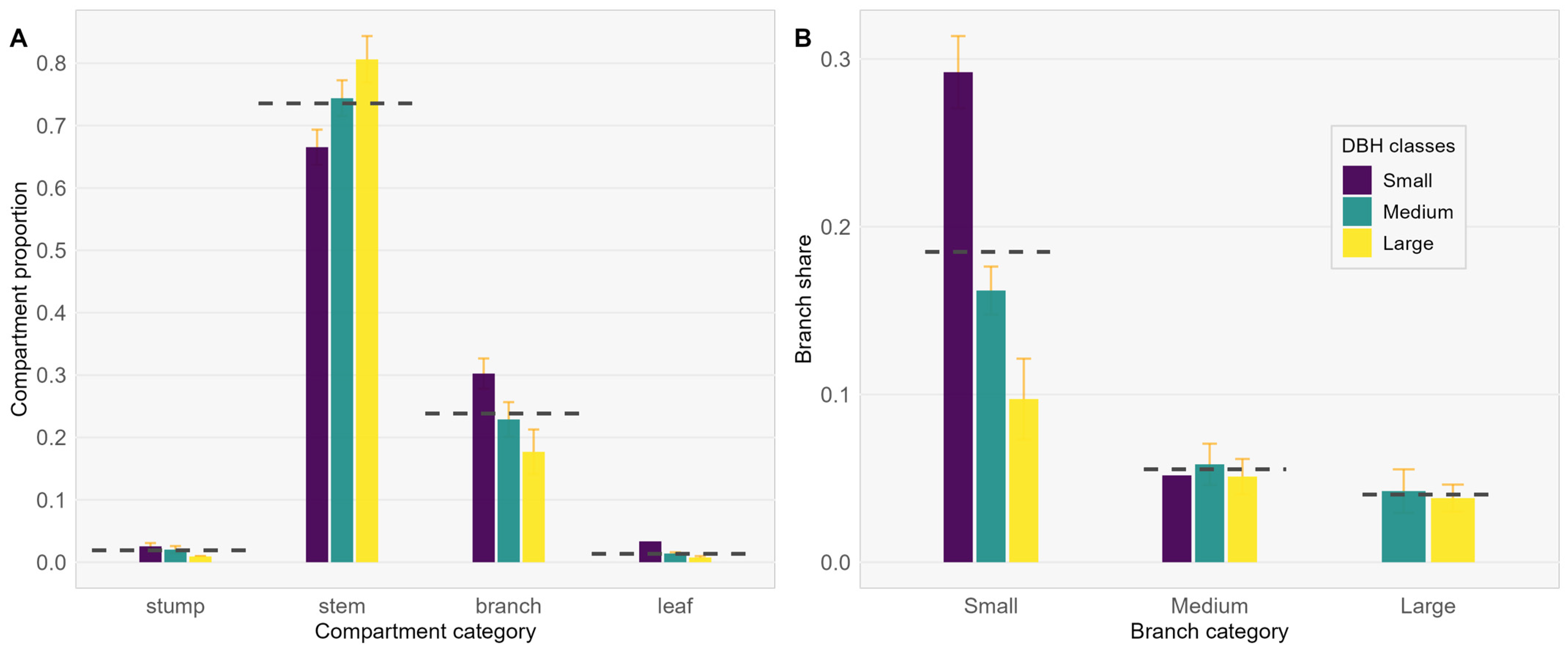
3.1. Variation of Wood Density among Tree Compartments and AGB Allocation

The average density of stem wood was 569.18 kg/m3 (SD ± 31.4, n = 172), whereas the average density of branch wood was 597.51 kg/m3 (SD ± 39.8, n = 50). This difference was statistically significant and large (difference = −28.33, 95% CI [−40.54, −16.13], t(67.65) = −4.63, p < 0.001) (Table 1 and Figure 2A). Additionally, the overall weighted wood stem and branch density (WWDst_br) had a value of 578.6 kg/m3 (Table 1). Significant differences were found between branches in the small category and stem as well as the medium branch category and stem (p < 0.001) (Figure 2B). Regarding the WD corresponding to each branch category, no significant differences were found (Figure 2B). The coefficient of variation of WD was 6.1% for WDic, while it was 5.6% and 4.6% for WDDBH and WDBase, respectively. On average, the density obtained from WDic was 2% lower than that obtained from WDDBH but not significantly different (p < 0.05; Figure S1).
Overall, the trend along the tree height in WD for European beech trees showed a slight decrease in the middle of the tree, specifically towards the crown insertion zone, relative to the base, and a positive trend towards the stem tip (Figure 3). In terms of weighted stem density (WWD) and stem and branch weighted wood density (WWDst_br), there were no significant differences (Figure S1). On the other hand, the density at the base of the stem (WDBase) was not significantly different compared to the density at the breast height level (WDDBH) (Figure S1).
The proportion of stem biomass from total aboveground biomass for the small diameter class recorded lower values (66.5%) compared to the medium and large (74.4% and 80.6%, respectively) classes (Figure 4A). In contrast, in the branch category, for smaller diameters, the proportion was higher (i.e., 30.2%) compared to medium and large classes (i.e., 17.7% and 22.9%, respectively). With regard to the stump and leaf biomass proportions, both had a negative trend with increasing diameter. The overall proportion for the stem category was 73.5%, while it was 23.8% for the branch category. Stump and leaf recorded the lower values in overall biomass allocation (1.9% and 1.3%, respectively) (Figure 4A). In terms of branch biomass allocation, the biomass for small branch categories decreased with increasing diameter classes from 29.2% to 9.7%. In the medium-sized branch class, all diameter classes had a proportion of around 5%, while in the large branch category, the proportion was around 4% and only present in the medium and large tree classes of diameters (Figure 4B). Overall, the relationship between DBH and the proportion of each compartment did not demonstrate statistical significance, although an association could be seen (Figure 4A).

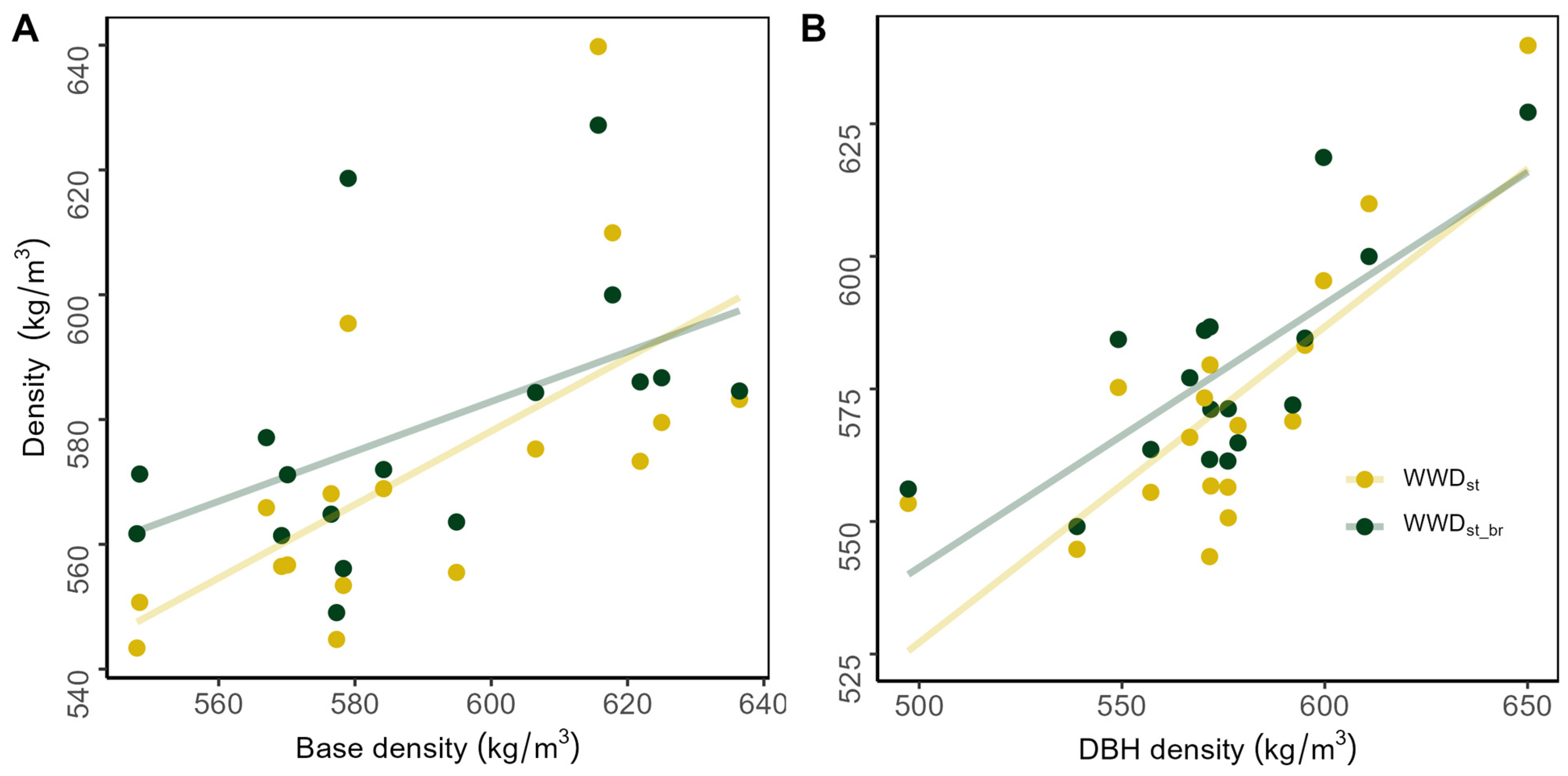
3.2. Weighted Wood Density Model Fitting

The equation coefficients to determine weighted stem density (WWDst) as well as weighted stem and branch densities (WWDst_br) are presented in Table 2. A total of 12 test models were run with densities at different levels (i.e., WDBase, WDDBH, and WDic), including DBH, as independent variables. The best performance of the models was recorded for model 2 (R2 = 0.669, AIC = 145.76), model 4 (R2 = 0.652, AIC = 146.60), and model 10 (R2 = 0.611, AIC = 142.880). The WDDBH played a significant role in deriving the weighted wood densities for all models (p < 0.01; Table 2). Models that did not produce good results in determining both WWDst and WWDst_br were the ones that included WDic as an independent variable (i.e., models 5, 6, 11, and 12; Table 2). In order to test the performance of weighted tree density in assessing aboveground biomass (i.e., AGBestimated), the models that best explain the variability were selected (i.e., models 2, 4, and 10; Table 2). The WDDBH appeared to account for a greater portion of the variances observed in the weighted densities for both WWDst and WWDst_br (R2 = 0.60 and 0.58, respectively; Table 2 and Figure 5). In contrast, the densities at the base of the tree explained only 40% of the variability for WWDst and 26% for WWDst_br (Table 2).

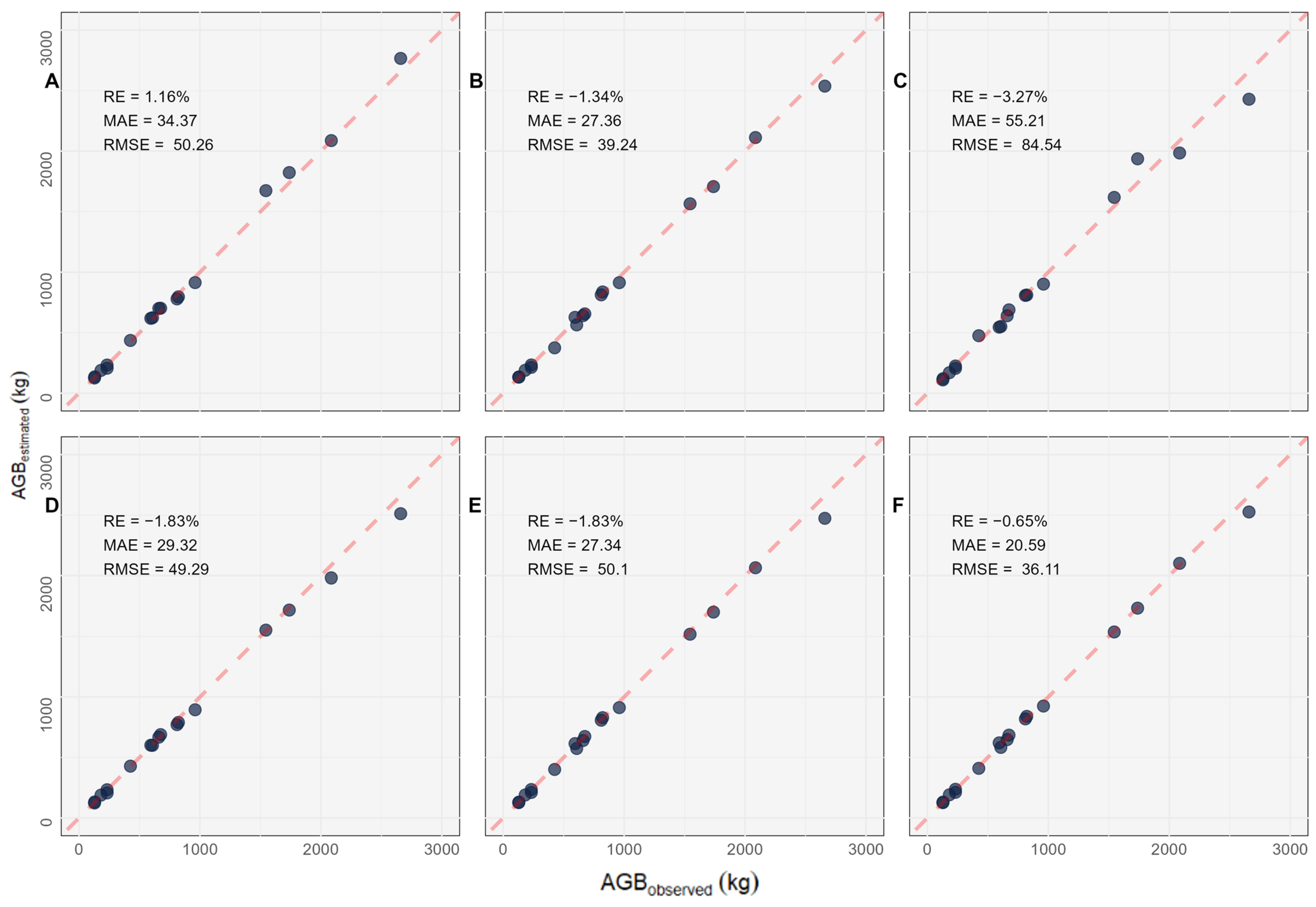
3.3. AGB Estimations Derived from Weighted Wood Densities

In the aboveground biomass assessment (i.e., AGBestimated), which was derived from the tree volume and WD at different levels as well as the weighted density where the output of the selected models was taken into account, a relatively constant difference in the bias estimation was observed. Using WDBase, an overestimation of 1.2% (RMSE = 50.3; Figure 6A) was observed compared to WDDBH, where the biomass was underestimated by −1.3% (RMSE = 39.2; Figure 6B), and WDic, where the biomass was underestimated by −3.3% (RMSE = 84.5; Figure 6C). Models 2 and 4 resulted in an underestimation of the volume by −1.8% (RMSE = 49.3 and 50.1, respectively; Figure 6D,E), while model 10, which had the lowest bias, resulted in an underestimation by −0.65% (RMSE = 36.1; Figure 6F).

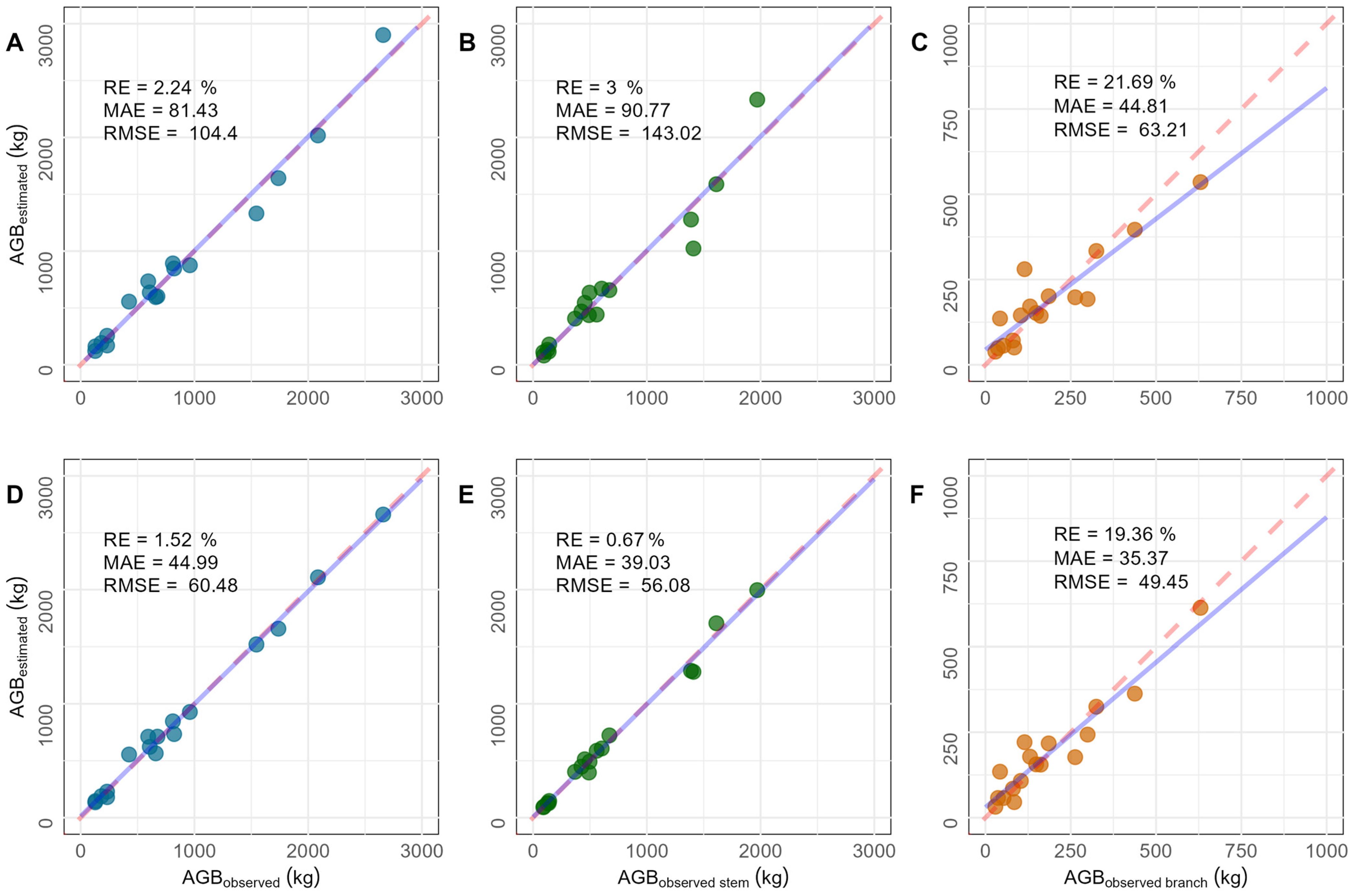
3.4. AGB Model Fitting

Two different sets of allometric equations were tested to determine the aboveground biomass using independent variables that can be easily measured in the field (i.e., DBH and height). The biomass prediction equation that took into account both DBH and H performed well in explaining the variability for total biomass (R2 = 0.993), stem biomass (R2 = 0.99), and branch biomass (R2 = 0.905). On the other hand, the prediction equation that considered only diameter explained 97.9% of the variance for the total biomass and 94% and 84.7% for stem and branch biomass, respectively (Table 3).
In Figure 7, a visual representation is presented showing a comparative analysis between the field measurement values of biomass (AGBobserved) and the corresponding biomass estimations obtained through the utilization of models 1–6 (Table 3).
By introducing height as a predictor in the models, a notable improvement was observed in biomass estimation for AGBtotal (RE = 1.5%, R2 = 0.993), AGBstem (RE = 0.7%, R2 = 0.990), and AGBbranch (RE = 19.4%, R2 = 0.905) (Table 3 and Figure 7). Moreover, the RMSE was 42% lower than the equation using just DBH as a predictor variable for AGBtotal, 60.8% for AGBstem, and 21.8% for AGBbranch. Although the R2 and RMSE improved for model 6, the effect of H was not statistically significant (p > 0.05; Table 3). The use of DBH alone overestimated branch biomass determination by 21.7%, stem biomass by 3%, and total aboveground biomass by 2.2% (Figure 7). The distribution of residuals in AGBtotal (i.e., for log-transformed values) was normally distributed both in the model that included DBH and height and the model with DBH as an independent variable (i.e., model 1—Shapiro–Wilk test, p = 0.781 > 0.05, model 2—Shapiro–Wilk test, p = 0.737 > 0.05; Figure S2).

4. Discussion

Estimating AGB and WD in various compartments of the tree for mountain beech forests is essential for developing carbon sequestration and forest management strategies aimed at mitigating climate change. The approaches carried out in this study were focused on two related aspects regarding wood density and biomass estimation. Firstly, we analyze the methods of determining the average WD, emphasizing the importance of adopting best practices in this calculation. Additionally, we investigated the variation of WD along the tree’s height and examined the distribution of AGB within different tree compartments. Furthermore, our research addressed the practical challenge of calibrating equations with simple, measurable predictors on the field (i.e., DBH and H) to estimate AGB accurately. Despite the fact that only one stand type was captured in this study with a relatively small number of trees (n = 17), the results may be locally representative for both density and allometry determination for European beech in mountainous areas. It should also be pointed out that the number of trees included in the leaf biomass analysis was limited (i.e., nine trees) due to the fact that some of them were analyzed outside the growing season.

4.1. Wood Density and AGB Allocation

The method of determining the weighted tree density has been used in several studies, such as those undertaken in temperate forests by Demol et al. [36], in the tropics by Sagang et al. [34], and in subtropical forests by Deng et al. [44]. The mean density values for stem density in European beech were marginally below the average value recommended by the IPCC [3]. Similar results have been obtained by Skovsgaard and Nord-Larsen for Danish beech forests [45], although the weighted WD value for stems and branches (WWDst_br) was 1.6% higher than the mean stem density. Also, WWDst had lower values on average compared to WDDBH. This is due to the fact that a slight decrease could be seen in wood density along the stem from the tree base towards the middle, which coincides with the crown insertion area (Figure 3). As for the mean density in branches, it had higher values reported by Skovsgaard and Nord-Larsen [45], compared to the average density per stem, contrary to Cienciala et al. [16], where the average value for branches was 560.1 kg/m3. The small but not statistically significant differences between WDic and WDDBH (Figure S1) may be due to the inclusion of bark in the wood core density assessment and the reduced number of samples assessed, especially for small class categories (Table 1). Consistent with this, such differences between WDic and WDDBH were also found by Demol et al. [36], even though, in this study, the bark was not introduced into the increment core density and only included in the discs provided at the DBH section. In this case, the data set presented here can be applied with caution, especially for mountain beech forests. In addition, the inter-tree variability of WD along the class diameter can be controlled by the genetic and environmental synergy (i.e., the “tree effect” [46]).
Analyzing the mean stem density by diameter categories, it was observed that the density of the stem (i.e., WDstem) was higher for trees with smaller diameters (Table 1). This could be considered a strategy of shade-tolerant species [47], where density allocation in younger trees is more pronounced [46], in order to gain resistance to biotic factors [48]. Higher density in the branch compartment than the stem compartment has also been found in other deciduous species [49], with this being attributed to the tension in the branches to support their own weight [50], which could also be the case for European beech. On the one hand, the effort to explain WD using just the wood cores in prediction models was unsuccessful as the estimated WDic failed to satisfactorily explain the variability of the weighted mean density (WWDst) (i.e., models 5, 6, 11, and 12; Table 2). This may be due to the relatively small size of the increment core, which may not be representative of the whole stem tree density [12] as well as the difficulties of reaching the pith [11]. On the other hand, collecting a better representative sample disc density from the breast height level as well as from the base of the tree through destructive methods performed better in explaining the variability of the weighted tree density (i.e., models 2, 4, and 10; Table 2).
Regarding the WD variation along the tree height, the results showed that the WD towards the top slightly increased, consistent with the results of Longuetaud et al. [51]. The average density at breast height level for the same species was on average 1.7% lower than that obtained from the Belgium forest stand by Demol et al. [36]. A data set presented by Martinez-Sancho et al. [52] across Europe found a higher basic wood density (597 kg/m3) in comparison with our study (579 kg/m3; Table 1).
Concerning the proportion of tree biomass for each compartment, the overall stem proportion of biomass (73.5%) from the total AGB was slightly lower than in Vejpustková et al. [25], where biomass accounted for 82% for mature trees. However, for the large class of DBH, the results were comparable regarding stem biomass allocation (80.6% for our study) and also closer to Cienciala et al. [16] (85%). Despite there being changes in biomass allocation in each compartment relative to tree growth, our observations merely showed an increase in stem biomass and a decrease in branch biomass with an increase in the size of beech tree DBH. However, both the patterns of stem and branch biomass partitioning relative to the tree diameters were only marginally significant (p = 0.09 and p = 12).
Although these observations did not reach statistical significance in our study, they nevertheless align with the results obtained by Vejpustková et al. [25]. It is important to highlight that our study area consists of mature European beech trees in an uneven-aged stand. The trend of decreasing branch share with increasing DBH size may be attributed to the self-thinning of lower branches and diminished growth rates over time due to tree-ring accumulation. Furthermore, the branch biometry (i.e., mean and maximum length and diameter) increases considerably with local tree competition caused by the rate of mortality or intensity of thinning [53]. Considering the AGB prediction using weighted stem densities based on parameterized WD as independent variables (i.e., WDBase, WDDBH, and WDic) and tree size measurements (DBH) (i.e., models 2, 4, and 6; Table 2 and Figure 6D–F) as well as mean densities on the base and breast height level (i.e., Figure 6A–C), the best performance for WWDst_br estimation was achieved using model 10, where the underestimation was −0.65%. In comparison, the AGB from wood core density was underestimated by roughly 3.3% (Figure 6C). Thus, by using an expeditious method of determining tree biomass with increment cores, the rate of introducing errors can increase, particularly when dealing with small sample sizes and with substantial variability in increment core density. Additionally, errors can occur from potential water loss in increment core samples. In contrast, disc samples seem to be a better representation for assessing wood density. Indeed, research conducted in different tropical forests [54] suggests that sampling between 30 and 60 trees produces a reliable estimation of WD. On the other hand, a prior study in European beech forests [36] utilized only five harvested beech trees to quantify the vertical WD variation.

4.2. AGB Model Fitting

For modeling the total biomass of the trees as well as that of the stem and branches, a log-transform method was considered, where it was necessary to adjust the data with a correction factor (CF) considering backward transformation due to the deformation of the original data [21,41]. The allometric equations based on tree size characteristics (i.e., DBH and height) [13,14,21,26] used in the study achieved good results, both for AGBtotal and AGBstem, but with poorer accuracy results regarding AGBbranch [16,25], both with DBH and tree height and DBH. Tree height is used as a predictor variable in addition to diameter to reduce the estimation error [21,24,55]. Thus, the inclusion of height in the model led to a reduction in the overestimation of total AGBtotal from 2.2% to 1.5% compared to the model using only the diameter (Figure 7A,D). Moreover, the underestimation of the AGBstem and AGBbranch went from 3% to 0.7% and from 21.7% to 19.4%, respectively, by including the predictor H (Figure 7B,C,E,F). The stand structure and architecture of the European beech tree can have an influence on branch biomass [25]. Thus, the large variations in AGBbranch can be explained using different predictors like crown length or crown ratio [56,57] or even predictors associated with inter-tree competition, like tree social status [25].
All selected models from the literature performed satisfactorily in biomass prediction. However, the model proposed by Cienciala et al. [16] to predict the total biomass seems to have the lowest bias, while there was a high underestimation of around −8.6% with the model proposed by Vejpustková et al. [25] (Figure 8 and Table 4).
Note that the models proposed by Vejpustková et al. [25], underestimated the volume for AGBtotal as well as AGBstem and AGBbranch (Table 4). One reason for this may be the fact that stump biomass was not included in that study. Although the consideration of stumps as a part of aboveground biomass is very scarce in the literature of allometric models, its inclusion in our models increased the value of our data set by increasing the accuracy of the estimation of carbon stored in trees. Stump is considered a longer-term storage element compared to the foliage section [16] and can reach up to 2% of stem volume, especially for trees with a large diameter [58]. Improvement of biomass estimation by including other variables, such as the site index or the type of silvicultural interventions implemented [59,60] as well as the tree status, could be of interest for future studies; they were not taken into account in this study due to cost implications and a lack of human resources.
Our allometric equations should be applied cautiously, particularly in biomass estimation for trees grown in extreme conditions, trees grown isolated at the edge of stands, and solitary trees [16]. Such trees invest more resources (higher biomass allocation rate) into the development of crowns (e.g., branches), while our data were collected from trees sampled under good site conditions and from closed canopy stands.
However, it is important to recognize several limitations of our study, which may reduce the robustness and accuracy of our findings in carbon estimation. First, there were a limited number of sampled trees for which we collected the leaves. For coniferous species, the sampling moment is not important, but for deciduous species, it is crucial to concentrate all efforts on leaf sampling around the peak time of complete foliar system development in order to avoid the extreme time periods when the leaves are either not fully developed or have started to fall. Secondly, considering the amount of carbon sequestered in the soil (especially in the root system), it is fundamental to build allometric equations to estimate the belowground biomass. Nevertheless, the large amount of effort and time needed for root sampling meant there are a limited number of existing studies related to belowground biomass estimations. For this reason, even with a very small sample size, such studies will be very valuable in the near future, especially because the health of forest soils has started to become a key element in the mitigation of negative climate change consequences and the importance of roots in the carbon cycle of forest ecosystems is well proven and recognized. Moreover, by including additional sites (e.g., altitude [25]) or stand predictors (e.g., stand age [49,61], stand structure, or stand index [16,25]), better fitting experimental data can be obtained compared to very simple classical allometric models (based only on DBH and/or height).

5. Conclusions

Our findings may have practical applications, especially in the context of carbon inventory. The equations we developed for determining tree density and biomass can be adaptable and can be applied, at least with precautions, in beech forests, especially in mountainous regions. Depending on the type of data available, i.e., whether it includes specific volume measurements or basic tree metrics, the methodology can be effectively utilized for other sites with beech trees.
In order to avoid biases, the significant differences found between densities of stems and branches should be taken into account for the correct estimation of total AGB. A slight decrease in density along the stem was observed in the middle of the tree relative to the base, followed by an increase towards the top of the tree. The biomass distribution among the tree compartments showed variation with tree growth, resulting in a reduced share of biomass in branches with an increase in tree diameter. Nevertheless, estimating biomass using the weighted density of stems and branches yielded more accurate and reliable estimates compared to other approaches, thus giving better results in estimating the carbon stock of European beech. To estimate the weighted density of a tree in a more practical way, we showed that it was possible to use densities collected at the base and at the breast height level to determine the weighted density with accurate results when using DBH as a predictor. Also, for a practical approach to estimating the aboveground biomass of a tree, allometric equations for beech were parameterized based on independent variables that are easy to measure in the field and have applicability to different ranges of diameters.
As an alternative solution, the sampling strategy adopted in the present study based on increment cores at the DBH section could be empirically developed for beech forests in mountainous regions. Further, to obtain full confirmation of our results, beech WD and AGB allocation studies using field biomass measurements should be extended to different regions in the Carpathian Mountains.

Supplementary Materials

The following supporting information can be downloaded at: https://www.mdpi.com/article/10.3390/f15030404/s1, Table S1: General characteristics and aboveground biomass estimation in each compartment of the sampled trees; Figure S1: Wood density comparison; Figure S2: Q–Q plot of aboveground biomass (i.e., AGBtotal) estimation using allometric equations from model 1 (A) and model 2 (B).

Author Contributions

Conceptualization, G.R.R., C.I.B., S.P. and I.C.P.; methodology, S.P., G.R.R., C.I.B., A.B.C., T.S., A.Z., D.P. and G.I.; software, S.P. and G.R.R.; validation, G.R.R., I.C.P. and C.I.B.; formal analysis, S.P. and C.I.B.; investigation, G.R.R. and I.C.P.; resources, S.P., G.R.R. and C.I.B.; data curation, S.P.; writing—original draft preparation, S.P., G.R.R. and C.I.B.; writing—review and editing, S.P., G.R.R., C.I.B. and I.C.P.; visualization, G.R.R., S.P. and C.I.B.; supervision, G.R.R., C.I.B. and I.C.P.; project administration, G.R.R., S.P. and C.I.B.; funding acquisition, G.R.R., S.P. and I.C.P. All authors have read and agreed to the published version of the manuscript.

Funding

The research was supported by “Marin Drăcea”, the National Institute for Research and Development in Forestry, through the project PN 23090203; partially through the Contract 47/N/2019 with the Ministry of Water Environment and Forests; partially by the “Transilvania” University of Brasov and partially through the project “Optimizarea deciziilor de management silvic pentru un viitor cu emisii reduse de carbon şi rezilienţă climatică în Europa” (contract 35PHE/2024).

Data Availability Statement

The data presented in this study are available on request from the corresponding author.

Acknowledgments

The authors would like to thank the forest monitoring team of “Marin Drăcea”, the National Institute for Research and Development in Forestry; the Forest Management Department; and the involved staff from Experimental Base Săcele for the proper conduct and coordination of field operations. Moreover, we thank the members involved in the density analysis in the laboratory of the Brașov Station Research Institute.

Conflicts of Interest

The authors declare no conflicts of interest.

References

  1. Bastin, J.-F.; Finegold, Y.; Garcia, C.; Mollicone, D.; Rezende, M.; Routh, D.; Zohner, C.M.; Crowther, T.W. The Global Tree Restoration Potential. Science 2019, 365, 76–79. [Google Scholar] [CrossRef]
  2. Church, J.; Clark, P.; Cazenave, A.; Gregory, J.; Jevrejeva, S.; Levermann, A.; Merrifield, M.; Milne, G.; Nerem, R.; Nunn, P.; et al. Climate Change 2013: The Physical Science Basis. Contribution of Working Group I to the Fifth Assessment Report of the Intergovernmental Panel on Climate Change; Cambridge University Press: Cambridge, UK, 2013; pp. 1138–1191. [Google Scholar]
  3. IPCC Intergovernmental Panel on Climate Change. 2006 IPCC Guidelines for National Greenhouse Gas Inventories; Institute for Global Environmental Strategies: Hayama, Japan, 2006. [Google Scholar]
  4. Wassenberg, M.; Chiu, H.-S.; Guo, W.; Spiecker, H. Analysis of Wood Density Profiles of Tree Stems: Incorporating Vertical Variations to Optimize Wood Sampling Strategies for Density and Biomass Estimations. Trees 2015, 29, 551–561. [Google Scholar] [CrossRef]
  5. UNFCCCC. Report of the Conference of the Parties on Its Thirteenth Session, Held in Bali from 3 to 15 December 2007. In Proceedings of the Addendum. Part Two: Action taken by the Conference of the Parties at its thirteenth session Decisions adopted by the Conference of the Parties, Bali, Indonesia, 3–15 December 2008. [Google Scholar]
  6. Shi, L.; Liu, S.; Shi, L.; Liu, S. Methods of Estimating Forest Biomass: A Review; IntechOpen: London, UK, 2017; ISBN 978-953-51-2938-7. [Google Scholar]
  7. Flores, O.; Coomes, D.A. Estimating the Wood Density of Species for Carbon Stock Assessments. Methods Ecol. Evol. 2011, 2, 214–220. [Google Scholar] [CrossRef]
  8. MacFarlane, D.W. Functional Relationships Between Branch and Stem Wood Density for Temperate Tree Species in North America. Front. For. Glob. Chang. 2020, 3, 63. [Google Scholar] [CrossRef]
  9. King, D.A.; Davies, S.J.; Tan, S.; Noor, N.S.M. The Role of Wood Density and Stem Support Costs in the Growth and Mortality of Tropical Trees. J. Ecol. 2006, 94, 670–680. [Google Scholar] [CrossRef]
  10. Van Gelder, H.A.; Poorter, L.; Sterck, F.J. Wood Mechanics, Allometry, and Life-History Variation in a Tropical Rain Forest Tree Community. New Phytol. 2006, 171, 367–378. [Google Scholar] [CrossRef]
  11. Gao, S.; Wang, X.; Wiemann, M.C.; Brashaw, B.K.; Ross, R.J.; Wang, L. A Critical Analysis of Methods for Rapid and Nondestructive Determination of Wood Density in Standing Trees. Ann. For. Sci. 2017, 74, 1–13. [Google Scholar] [CrossRef]
  12. Wiemann, M.C.; Williamson, G.B. Biomass Determination Using Wood Specific Gravity from Increment Cores; General Technical Report, FPL-GTR-225; USDA Forest Service, Forest Products Laboratory: Madison, MI, USA, 2013; 9p. [Google Scholar] [CrossRef]
  13. Parresol, B.R. Assessing Tree and Stand Biomass: A Review with Examples and Critical Comparisons. For. Sci. 1999, 45, 573–593. [Google Scholar]
  14. Chave, J.; Andalo, C.; Brown, S.; Cairns, M.A.; Chambers, J.Q.; Eamus, D.; Fölster, H.; Fromard, F.; Higuchi, N.; Kira, T.; et al. Tree Allometry and Improved Estimation of Carbon Stocks and Balance in Tropical Forests. Oecologia 2005, 145, 87–99. [Google Scholar] [CrossRef]
  15. Kuyah, S.; Mbow, C.; Sileshi, G.W.; van Noordwijk, M.; Tully, K.L.; Rosenstock, T.S. Quantifying Tree Biomass Carbon Stocks and Fluxes in Agricultural Landscapes. In Methods for Measuring Greenhouse Gas Balances and Evaluating Mitigation Options in Smallholder Agriculture; Springer: Berlin/Heidelberg, Germany, 2016; pp. 119–134. [Google Scholar]
  16. Cienciala, E.; Černý, M.; Apltauer, J.; Exnerová, Z. Biomass Functions Applicable to European Beech. J. For. Sci. 2005, 51, 147–154. [Google Scholar] [CrossRef]
  17. Repola, J. Models for Vertical Wood Density of Scots Pine, Norway Spruce and Birch Stems, and Their Application to Determine Average Wood Density. Silva Fenn. 2006, 40, 673–685. [Google Scholar] [CrossRef]
  18. Liepins, J.; Liepins, K. Mean Basic Density and Its Axial Variation in Scots Pine, Norway Spruce and Birch Stems. Res. Rural Dev. 2017, 1, 21–27. [Google Scholar]
  19. Repola, J. Biomass Equations for Birch in Finland. Silva Fenn. 2008, 42, 605–624. [Google Scholar] [CrossRef]
  20. Repola, J. Biomass Equations for Scots Pine and Norway Spruce in Finland. Silva Fenn. 2009, 43, 625–647. [Google Scholar] [CrossRef]
  21. Dutcă, I.; Zianis, D.; Petrițan, I.C.; Bragă, C.I.; Ștefan, G.; Yuste, J.C.; Petrițan, A.M. Allometric Biomass Models for European Beech and Silver Fir: Testing Approaches to Minimize the Demand for Site-Specific Biomass Observations. Forests 2020, 11, 1136. [Google Scholar] [CrossRef]
  22. Williamson, G.B.; Wiemann, M.C. Measuring Wood Specific gravity…Correctly. Am. J. Bot. 2010, 97, 519–524. [Google Scholar] [CrossRef] [PubMed]
  23. Somogyi, Z.; Cienciala, E.; Mäkipää, R.; Muukkonen, P.; Lehtonen, A.; Weiss, P. Indirect Methods of Large-Scale Forest Biomass Estimation. Eur. J. For. Res. 2007, 126, 197–207. [Google Scholar] [CrossRef]
  24. Ketterings, Q.M.; Coe, R.; van Noordwijk, M.; Ambagau’, Y.; Palm, C.A. Reducing Uncertainty in the Use of Allometric Biomass Equations for Predicting Above-Ground Tree Biomass in Mixed Secondary Forests. For. Ecol. Manag. 2001, 146, 199–209. [Google Scholar] [CrossRef]
  25. Vejpustková, M.; Zahradník, D.; Cihak, T.; Srámek, V. Models for Predicting Aboveground Biomass of European Beech (Fagus sylvatica L.) in the Czech Republic. J. For. Sci. 2015, 61, 2015–2045. [Google Scholar] [CrossRef]
  26. Zianis, D.; Mencuccini, M. Aboveground Biomass Relationships for Beech (Fagus moesiaca Cz.) Trees in Vermio Mountain, Northern Greece, and Generalised Equations for Fagus sp. Ann. For. Sci. 2003, 60, 439–448. [Google Scholar] [CrossRef]
  27. Șofletea, N.; Curtu, L. Dendrologie; Editura Universitatii Transilvania: Brasov, Romania, 2007; ISBN 978-973-635-885-2. [Google Scholar]
  28. Romanian National Forest Inventory (NFI). Available online: www.roifn.ro/site (accessed on 24 July 2023).
  29. National Inventory Report (NIR)-Romania. Available online: www.unfccc.int/documents/274077 (accessed on 24 July 2023).
  30. Decei, I. Contribuții La Cunoașterea Densității Lemnului. Revista Pădurilor 1987, 2, 77–80. [Google Scholar]
  31. Schad, P. World Reference Base for Soil Resources—Its Fourth Edition and Its History. J. Plant Nutr. Soil Sci. 2023, 186, 151–163. [Google Scholar] [CrossRef]
  32. Harris, I.; Osborn, T.; Jones, P.; Lister, D. Version 4 of the CRU TS Monthly High-Resolution Gridded Multivariate Climate Dataset. Sci. Data 2020, 7, 109. [Google Scholar] [CrossRef] [PubMed]
  33. Cornelissen, J.H.C.; Lavorel, S.; Garnier, E.; Díaz, S.; Buchmann, N.; Gurvich, D.E.; Reich, P.B.; Ter Steege, H.; Morgan, H.D.; Van Der Heijden, M.G.A.; et al. A Handbook of Protocols for Standardised and Easy Measurement of Plant Functional Traits Worldwide. Aust. J. Bot. 2003, 51, 335–380. [Google Scholar] [CrossRef]
  34. Sagang, L.B.T.; Momo, S.T.; Libalah, M.B.; Rossi, V.; Fonton, N.; Mofack, G.I.; Kamdem, N.G.; Nguetsop, V.F.; Sonké, B.; Ploton, P.; et al. Using Volume-Weighted Average Wood Specific Gravity of Trees Reduces Bias in Aboveground Biomass Predictions from Forest Volume Data. For. Ecol. Manag. 2018, 424, 519–528. [Google Scholar] [CrossRef]
  35. Schüller, E.; Martínez-Ramos, M.; Hietz, P. Radial Gradients in Wood Specific Gravity, Water and Gas Content in Trees of a Mexican Tropical Rain Forest. Biotropica 2013, 45, 280–287. [Google Scholar] [CrossRef]
  36. Demol, M.; Calders, K.; Krishna Moorthy, S.M.; Van den Bulcke, J.; Verbeeck, H.; Gielen, B. Consequences of Vertical Basic Wood Density Variation on the Estimation of Aboveground Biomass with Terrestrial Laser Scanning. Trees 2021, 35, 671–684. [Google Scholar] [CrossRef]
  37. Goslee, K.; Walker, S.M.; Grais, A.; Murray, L.; Casarim, F.; Brown, S. Module C-CS: Calculations for Estimating Carbon Stocks. In Leaf Technical Guidance Series for the Development of a Forest Carbon Monitoring System for REDD+; Winrock International: Little Rock, AR, USA, 2016. [Google Scholar]
  38. Walker, S.M.; Murray, L.; Tepe, T. Allometric Equation Evaluation Guidance Document; Winrock International: North Little Rock, AR, USA, 2016. [Google Scholar]
  39. Schumacher, H. Logarithmic Expression of Timber-Tree Volume. J. Agric. Res. 1933, 47, 719–734. [Google Scholar]
  40. Jenkins, J.C.; Chojnacky, D.C.; Heath, L.S.; Birdsey, R.A. National Scale Biomass Estimators for United States Tree Species. For. Sci. 2003, 49, 12–35. [Google Scholar] [CrossRef]
  41. Sprugel, D.G. Correcting for Bias in Log-Transformed Allometric Equations. Ecology 1983, 64, 209–210. [Google Scholar] [CrossRef]
  42. Sakamoto, Y.; Ishiguro, M.; Kitagawa, G. Akaike Information Criterion Statistics. Dordr. Neth. D. Reidel 1986, 81, 26853. [Google Scholar]
  43. R Core Team. R: A Language and Environment for Statistical Computing; v4.3.2; R Foundation for Statistical Computing: Vienna, Austria, 2021. [Google Scholar]
  44. Deng, X.; Zhang, L.; Lei, P.; Xiang, W.; Yan, W. Variations of Wood Basic Density with Tree Age and Social Classes in the Axial Direction within Pinus massoniana Stems in Southern China. Ann. For. Sci. 2014, 71, 505–516. [Google Scholar] [CrossRef]
  45. Skovsgaard, J.P.; Nord-Larsen, T. Biomass, Basic Density and Biomass Expansion Factor Functions for European Beech (Fagus sylvatica L.) in Denmark. Eur. J. For. Res. 2011, 131, 1035–1053. [Google Scholar] [CrossRef]
  46. Bouriaud, O.; Bréda, N.; Le Moguédec, G.; Nepveu, G. Modelling Variability of Wood Density in Beech as Affected by Ring Age, Radial Growth and Climate. Trees 2004, 18, 264–276. [Google Scholar] [CrossRef]
  47. Chave, J.; Coomes, D.; Jansen, S.; Lewis, S.L.; Swenson, N.G.; Zanne, A.E. Towards a Worldwide Wood Economics Spectrum. Ecol. Lett. 2009, 12, 351–366. [Google Scholar] [CrossRef]
  48. Plourde, B.T.; Boukili, V.K.; Chazdon, R.L. Radial Changes in Wood Specific Gravity of Tropical Trees: Inter- and Intraspecific Variation during Secondary Succession. Funct. Ecol. 2015, 29, 111–120. [Google Scholar] [CrossRef]
  49. Liepiņš, K.; Liepiņš, J.; Ivanovs, J.; Bārdule, A.; Jansone, L.; Jansons, Ā. Variation in the Basic Density of the Tree Components of Gray Alder and Common Alder. Forests 2023, 14, 135. [Google Scholar] [CrossRef]
  50. Dahle, G.A.; Grabosky, J.C. Variation in Modulus of Elasticity (E) along Acer platanoides L. (Aceraceae) Branches. Urban For. Urban Green. 2010, 9, 227–233. [Google Scholar] [CrossRef]
  51. Longuetaud, F.; Mothe, F.; Santenoise, P.; Diop, N.; Dlouha, J.; Fournier, M.; Deleuze, C. Patterns of Within-Stem Variations in Wood Specific Gravity and Water Content for Five Temperate Tree Species. Ann. For. Sci. 2017, 74, 1–19. [Google Scholar] [CrossRef]
  52. Martínez-Sancho, E.; Slámová, L.; Morganti, S.; Grefen, C.; Carvalho, B.; Dauphin, B.; Rellstab, C.; Gugerli, F.; Opgenoorth, L.; Heer, K.; et al. The GenTree Dendroecological Collection, Tree-Ring and Wood Density Data from Seven Tree Species across Europe. Sci Data 2020, 7, 1. [Google Scholar] [CrossRef]
  53. Pretzsch, H.; Rais, A. Wood Quality in Complex Forests versus Even-Aged Monocultures: Review and Perspectives. Wood Sci. Technol. 2016, 50, 845–880. [Google Scholar] [CrossRef]
  54. Pascoa, K.; Gomide, L.; Tng, D.; Scolforo, J.; Ferraz Filho, A.; Mello, J. How Many Trees and Samples Are Adequate for Estimating Wood-Specific Gravity across Different Tropical Forests? Trees 2020, 34, 1383–1395. [Google Scholar] [CrossRef]
  55. Feldpausch, T.R.; Lloyd, J.; Lewis, S.L.; Brienen, R.J.W.; Gloor, M.; Monteagudo Mendoza, A.; Lopez-Gonzalez, G.; Banin, L.; Abu Salim, K.; Affum-Baffoe, K.; et al. Tree Height Integrated into Pantropical Forest Biomass Estimates. Biogeosciences 2012, 9, 3381–3403. [Google Scholar] [CrossRef]
  56. Cienciala, E.; Apltauer, J.; Exnerová, Z.; Tatarinov, F. Biomass Functions Applicable to Oak Trees Grown in Central-European Forestry. J. For. Sci. 2008, 54, 109–120. [Google Scholar] [CrossRef]
  57. Cienciala, E.; Černý, M.; Tatarinov, F.; Apltauer, J.; Exnerová, Z. Biomass Functions Applicable to Scots Pine. Trees 2006, 20, 483–495. [Google Scholar] [CrossRef]
  58. Pařez, J.; Žlábek, I.; Kopřiva, J. Basic Technical Units of Determining Timber Volume in the Logging Fund of the Main Forest Species. Forestry 1990, 479–508. [Google Scholar]
  59. Bouriaud, O.; Don, A.; Janssens, I.A.; Marin, G.; Schulze, E.-D. Effects of Forest Management on Biomass Stocks in Romanian Beech Forests. For. Ecosyst. 2019, 6, 19. [Google Scholar] [CrossRef]
  60. Noormets, A.; Epron, D.; Domec, J.C.; McNulty, S.G.; Fox, T.; Sun, G.; King, J.S. Effects of Forest Management on Productivity and Carbon Sequestration: A Review and Hypothesis. For. Ecol. Manag. 2015, 355, 124–140. [Google Scholar] [CrossRef]
  61. Xue, Y.; Yang, Z.; Wang, X.; Lin, Z.; Li, D.; Su, S. Tree Biomass Allocation and Its Model Additivity for Casuarina equisetifolia in a Tropical Forest of Hainan Island, China. PLoS ONE 2016, 11, e0151858. [Google Scholar] [CrossRef]
Figure 1. Study location map at the country level (A) and visual representation of sampling measurements for WD and volume section log calculations (B). In (A), the dark dot represents the study area, and the light brown area represents the boundary of Brasov County. In (B), black dotted rectangles represent the position of the collected sample discs for WD analysis; ρ 1 ρ n are sample densities of each beginning of section logs, while ρ m 1 ... ρ m n are mean log densities used for biomass estimation; ρ < 5 ,   ρ 5 12 , and ρ > 12 represent sample branch densities for each specific size category (i.e., small, medium, and large categories); D0…D7 represent the diameters taken at 10, 30, 50, 100, 130, 200, 250, and 300 cm (gray arrows); D8…Dn represent the diameters taken at intervals of 1 m until the stem top (diameter of 5 cm); V0 is the estimated stump volume; and V1…Vn are the stem section volumes computed through Smalian’s method.
Forests 15 00404 g001
Figure 2. Box-plots of wood density for stem and branch estimated from samples (A) and for stem and each branch category (i.e., small, medium, and large branch categories) (B). Different letters represent significant differences at the p < 0.05 probability level (Tukey’s test).
Forests 15 00404 g002
Figure 3. WD variation along relative tree sample height. The best fit line (i.e., smoothed line using the Loess method with a span value of 1) for WD is represented by the blue line, and the light gray color represents the 95% confidence interval. The dotted black horizontal line represents the mean WD, while the vertical dotted brown line represents the mean first living branch height (FLBH).
Forests 15 00404 g003
Figure 4. Proportions of aboveground biomass per each compartment (i.e., stump, stem, branch, leaves) with regard to three stem DBH classes (A) and branch proportions per each category (i.e., small, medium, and large branches) (B). Orange lines represent standard errors. Note. For AGB, the stump mass was estimated. The gray dotted line represents the mean overall component proportion for each category.
Forests 15 00404 g004
Figure 5. Linear relationship between weighted density and density at the base (WDBase) (A) and density at the 1.3 m aboveground (WDDBH) (B). The yellow line stands for weighted wood stem density (WWDst), while the green line stands for weighted wood stem and branch density (WWDst_br).
Forests 15 00404 g005
Figure 6. Graphical representation of estimated aboveground biomass (i.e., AGBestimated) against observed biomass (i.e., AGBobserved) considering different WDs. (A) prediction of biomass by density at the base (WDBase); (B) prediction of biomass by density at breast height (WDDBH); (C) prediction of biomass by increment core density (WDic); (D) prediction of biomass by weighted wood stem density (WWDst) using model 2; (E) prediction of biomass by WWDst using model 4; (F) prediction of biomass by WWDst_br using model 10. RE (mean relative bias, %), MAE (mean absolute error), and RMSE (root mean squared error) are metrics used to evaluate the accuracy of the regressions.
Forests 15 00404 g006
Figure 7. Graphical representation of predicted aboveground biomass (i.e., AGBestimated) against observed biomass (i.e., AGBobserved) using allometric equations. Each dot color represents the predicted biomass for each component (i.e., blue dots = aboveground biomass; green dots = stem biomass; and orange dots = branch biomass). (AC) DBH used as a predictor (models 1, 3, and 5; Table 3); (DF) DBH and H used as predictors (models 2, 4, and 6; Table 3). The red dotted line is a 1:1 line, while the light blue line represents the regression line of predicted points. RE (mean relative bias, %), MAE (mean absolute error), and RMSE (root mean squared error) are metrics used to evaluate the accuracy of the regressions.
Forests 15 00404 g007
Figure 8. Aboveground biomass predicted using different equations from the literature (i.e., AGBestimated) against observed biomass (i.e., AGBobserved). (A) Aboveground biomass; (B) stem biomass; (C) branch biomass. The red dotted line represents the 1:1 line.
Forests 15 00404 g008
Table 1. Main sample tree characteristics of targeted trees.
Classes of DiametersNo. of TreesNo. of Stem Sample DiscsDBH
(cm)
Tree Height
(m)
FLBH
(m)
Tree Length
(m)
Basic WD (kg/m3 ± sd)
WDicWDstemWDDBHWDstumpWDbrWWDst_br
Small52419.4
(16.8–22.3)
15.3
(13.3–16.5)
7.3
(3.4–13.5)
11.6
(9–13.6)
546 ± 21590 ± 36602 ± 31592 ± 23595 ± 53596 ± 28
Medium89433.0
(30.1–36.0)
23.2
(20.6–27.4)
8.3
(4.4–10.7)
19.4
(16.0–23.2)
563 ± 33563 ± 31558 ± 29579 ± 27596 ± 41570 ± 13
Large45448.3
(42.0–56.5)
32.1
(30.2–33.5)
13.1
(6.5–23.2)
29.7
(28.5–31.0)
584 ± 47572 ± 25575 ±16606 ± 30602 ± 30574 ± 13
Total1717232.6
(16.8–56.5)
22.9
(13.3–33.5)
9.1
(3.4–23.2)
19.5
(9.0–31.0)
563 ± 35569 ± 31575 ± 32589 ± 27598 ± 40579 ± 21
DBH is the diameter at breast height in cm. Tree height is the total tree height in m. FLBH is the first living branch height in m. Tree length represents the stem length in m from the base to a diameter less than 5 cm. WDic, WDstem, WDDBH, WDstump, WDbr, and WWDst_br represent the mean increment core density, mean stem density, mean density at breast height diameter, mean stump density, mean branch density, and weighted wood density of stems and branches, respectively. The values within brackets represent the minimum and maximum values corresponding to each class of diameters.
Table 2. Prediction models for weighted wood stem density (WWDst, kg/m3) and weighted wood stem and branch density (WWDst_br, kg/m3).
PredictorModel No.ModelModel ParametersModel Performance
a (Intercept)bcdeR2R2 adj.RSEAIC
WWDst1~a + b × WDBase225.0430.588 ** 0.4040.36419.88153.767
(−7.002–457.088)(0.195–0.982)
2~a + b × WDBase + c × DBH245.655 *0.617 ***−1.142 ** 0.6690.62215.33145.760
(65.085–426.225)(0.311–0.923)(−1.873–−0.411)
3~a + d × WDDBH229.399 ** 0.596 *** 0.5960.56916.37147.160
(73.958–384.839) (0.326–0.866)
4~a + c × DBH + d × WDDBH283.943 ** −0.5570.532 ** 0.6520.60315.72146.600
(114.964–452.923) (−1.348–0.235)(0.256–0.808)
5~a + e × WDic663.086 *** −0.1620.050−0.01325.09161.685
(444.278–881.894) (−0.550–0.226)
6~a + c × DBH + e × WDic650.985 *** −0.993 −0.0830.2390.13123.24159.909
(446.562–855.409) (−2.134–0.148) (−0.456–0.290)
WWDst_br7~a + b × WDBase343.009 **0.400 * 0.2600.21018.77151.821
(123.871–562.147)(0.028–0.771)
8~a + b × WDBase + c × DBH358.324 **0.421 *−0.848 * 0.4630.38716.54148.346
(163.499–553.149)(0.091–0.751)(−1.638–−0.059)
9~a + d × WDDBH292.935 *** 0.497 *** 0.5770.54914.18142.290
(158.271–427.599) (0.263–0.731)
10~a + c × DBH + d × WDDBH328.469 *** −0.3630.456 ** 0.6110.55514.09142.880
(176.989–479.948) (−1.072–0.347)(0.208–0.703)
11~a + e × WDic644.331 *** −0.1170.036−0.02821.42156.302
(457.562–831.099) (−0.448–0.214)
12~a + c × DBH + e × WDic635.236 *** −0.746 −0.0570.1850.06920.39155.450
(455.936–814.535) (−1.747–0.255) (−0.384–0.270)
The models use as independent variables the base density (WDBase, kg/m3), sample disc density at breast height level (WDDBH, kg/m3), increment core density (WDic, kg/m3), and diameter at breast height (DBH, cm). Each model received specific parameters and corresponding confidence intervals. The performance of the models was evaluated by R2, R2adj., RSE, and AIC. Values in bold represent the models used in further analysis. * p < 0.05, ** p < 0.01, *** p < 0.001.
Table 3. Allometric equation models used for biomass estimation (i.e., total aboveground, stem, and branch biomass).
Biomass ComponentModel no.Model StructureModel ParametersEquation Performance
a (Intercept)bcR2 R2 adj.RMSEAIC
AGBtotal1a × DBHb0.0749 ***2.6184 *** 0.9790.978104.397−11.531
2a × DBHb × Hc0.051 ***2.000 ***0.808 *0.9930.99160.479−16.793
AGBstem3a × DBHb0.0326 ***2.7698 *** 0.9400.936143.019−6.536
4a × DBHb × Hc0.0168 ***1.6953 ***1.4024 ***0.9900.98756.085−30.373
AGBbranch5a × DBHb0.0824 *2.1759 *** 0.8470.83663.21424.332
6a × DBHb × Hc0.15603.2318 **−1.37810.9050.89249.44724.105
The models use tree size characteristics (DBH, cm) and height (H, m) as independent variables; a, b and c are model parameters. For each model, parameters were estimated. Note: Model parameters were adjusted by applying the correction factor (CF) described in Dutcă et al. [21] (i.e., Equations (5) and (6)). The performance of the back-transformed equations was evaluated using R2, R2 adj., RMSE, and AIC. * p < 0.05, ** p < 0.01, *** p < 0.001.
Table 4. Biomass prediction equations used for comparison.
Author and YearBiomass ComponentEquation StructureEquation ParametersEquation Performance
a (Intercept)bcR2RMSEMAERE
Dutca et al. [21] (Equation (2))AGB~a × DBHb0.070332.63680-0.979107.2581.272.30
Dutca et al. [21] (Equation (3))~a × DBHb × Hc0.042502.146800.690900.99266.4650.34−2.61
Cienciala et al. [16] (Equation (3))AGB~a × DBHb × Hc0.047002.121000.697000.99361.6547.940.46
AGBstem0.014002.053001.084000.983123.1477.447.14
AGBbranch5.137002.66500−1.878000.84897.8166.5426.61
Vejpustková et al. [25] (Equation (DH3))AGB~a × DBHb × Hc0.009622.155401.137880.990115.1785.11−8.63
AGBstem0.005602.104251.291840.983125.5267.64−2.36
AGBbranch0.006112.355090.561040.82668.0048.25−2.14
Our equation (Equation (2))AGB~a × DBHb × Hc0.051141.999570.807670.99360.4844.991.52
AGBstem0.016771.695271.402360.99056.0839.030.67
AGBbranch0.156033.23183−1.378150.90549.4535.3719.36
The observed biomass (i.e., AGBobserved) was compared with prediction biomass equations from the literature. R2 = coefficient of determination, RMSE = root mean squared error, MAE = mean absolute error, and RE = mean relative bias in % are metrics used to evaluate the equations accuracy; a, b and c are model parameters. For each model, parameters were estimated. Note: The parameters for Dutcă et al. [21] equations have been adjusted with the correction factor (CF) for logarithmic back-transformation correction.
Disclaimer/Publisher’s Note: The statements, opinions and data contained in all publications are solely those of the individual author(s) and contributor(s) and not of MDPI and/or the editor(s). MDPI and/or the editor(s) disclaim responsibility for any injury to people or property resulting from any ideas, methods, instructions or products referred to in the content.

