Article

Assessment of the Potential of Indirect Measurement for Sap Flow Using Environmental Factors and Artificial Intelligence Approach: A Case Study of Magnolia denudata in Shanghai Urban Green Spaces

1
Precision Forestry Key Laboratory of Beijing, Beijing Forestry University, Tsinghua East Road, Beijing 100083, China
2
Shanghai Academy of Landscape Architecture Science and Planning, 899 Longwu Road, Shanghai 200433, China
*
Authors to whom correspondence should be addressed.
These authors contributed equally to this work.
Forests 2023, 14(9), 1768; https://doi.org/10.3390/f14091768
Submission received: 19 July 2023 / Revised: 25 August 2023 / Accepted: 30 August 2023 / Published: 31 August 2023
(This article belongs to the Special Issue Forest Hydrology under Climate Change)

Abstract

:
The measurement of plant sap flow has long been a traditional method for quantifying transpiration. However, conventional direct measurement methods are often costly and complex, thereby limiting the widespread application of tree sap flow monitoring techniques. The concept of a Virtual Measurement Instrument (VMI) has emerged in response to this challenge by combining simple instruments with Artificial Intelligence (AI) algorithms to indirectly assess specific measurement objects. This study proposes a tree sap flow estimation method based on environmental factors and AI algorithms. Through the acquisition of environmental factor data and the integration of AI algorithms, we successfully achieved indirect measurement of tree sap flow. Accounting for the time lag response of the flow to environmental factors, we constructed the Magnolia denudata sap flow estimation model using the K-Nearest Neighbor (KNN), Random Forest (RF), Backpropagation Neural Network (BPNN), and Long Short-Term Memory network (LSTM) algorithms. The research results showed that the LSTM model demonstrated greater reliability in predicting sap flow velocity, with R2 of 0.957, MAE of 0.189, MSE of 0.059, and RMSE of 0.243. The validation of the target tree yielded an R2 of 0.821 and an error rate of only 4.89% when applying the model. In summary, this sap flow estimation method based on environmental factors and AI provides new insights and has practical value in the field of tree sap flow monitoring.

1. Introduction

Root systems play a critical role in the physiological activities of plants, including their growth, development, temperature regulation, and nutrient transport [1,2,3]. Adequate water supply not only contributes to photosynthesis and dry matter accumulation, but also fulfills the basic nutrient requirements for healthy plant growth [4]. Most of the absorbed water is used for plant transpiration [5,6]. Due to growth rhythmicity, the water uptake efficiency of the plant root system shows cyclical variations in different seasons or at different times of the day [7]. Extensive research has been conducted to reveal the biological mechanisms involved in the above processes [3,8,9]. Measuring plant sap flow has long been a traditional method to quantify transpiration. Various techniques have been employed in this field, including the dye method, isotope tracing method, gravimetric method, magnetic fluid mechanic method, whole-tree container method, rapid weighing method, and heat technique [10,11,12,13]. In forest environments, traditional methods such as the whole-tree container method and rapid weighing method may introduce potential errors during sampling and measurement. In contrast, the heat technique has multiple advantages due to its high sensitivity, real-time monitoring capability, and relatively simple measurement procedures. It is worth noting that the heat technique supports digital modeling, automated data collection, storage, and multi-probe measurements at different time intervals [14]. This technique has become the preferred method for researchers in various application scenarios [15]. Currently, the widely adopted method involves the use of thermal dissipation probes (TDP), which are inserted into tree trunks to measure the voltage difference between the upper and lower probes. These measurements are calibrated and modeled based on known sap flow data, and the voltage signal changes are used to estimate tree sap flow rates [16]. Despite the great potential demonstrated by heat-based sap flow monitoring instruments in practical applications, their relatively high costs still limit their development. The manufacturing and maintenance costs of these instruments are high, and their power supply depends mainly on mains electricity or solar cells, which restricts their feasibility in large-scale and long-term monitoring applications. Even in extensive areas such as forests, there are still challenges in overcoming technical and resource limitations for widespread device installations. In addition, the process of acquiring sap flow data also faces challenges. Complex data preprocessing procedures and tedious calibration steps make it difficult to directly analyze and interpret the raw data collected from monitoring instruments. These data preprocessing steps may include noise filtering, data interpolation, and outlier handling, which require a significant amount of time and human resources. At the same time, instrument calibration needs to be regularly conducted to ensure the accuracy and reliability of sap flow data. All these factors, to some extent, reduce the efficiency of sap flow data acquisition. Therefore, finding an economically feasible and reliable plant sap flow monitoring method, particularly for third-world countries, is a highly meaningful research topic.
In our previous research, the concept of a virtual measuring instrument (VMI) was introduced [17]. As an innovative measurement device, the VMI combines the results of real measuring instruments with computer algorithms to simulate the measurement behavior of another instrument. Its uniqueness lies in its ability to simulate the effects of using expensive measuring instruments with relatively cheap or simple instruments. In recent years, the rapid development of artificial intelligence (AI) algorithms has brought new possibilities to VMI. Especially in dealing with large and complex data and conducting accurate simulations, AI has shown tremendous potential and advantages. According to VMI theory, we can transform the collection of sap flow data from traditional heat-based instrument measurements to estimation using more economical instruments combined with AI algorithms. Based on this theory, our research method is as follows: first, real sap flow data of certain trees are obtained using heat-based methods in specific areas; then, through feature engineering methods, we identify environmental factors that affect sap flow variations [18,19,20]. Finally, we build a sap flow estimation model based on AI algorithms. Then, we deploy simple instruments in other areas and apply the model we have established to obtain sap flow estimations for those areas. Therefore, to some extent, we can deploy micro-weather stations within a forest to obtain small-scale meteorological data. Even on a larger scale, we can consider spatial interpolation using rough meteorological station data or use remote sensing technology to obtain data of different resolutions. Ultimately, by utilizing the model we have established based on real data, we can estimate tree sap flow at different scales [21] (such as individual trees, entire forest stands, etc.).
In recent years, the rapid development of AI algorithms has introduced new possibilities for VMI. Especially in handling large and complex data and performing accurate simulations, AI has demonstrated great potential and advantages [22,23]. Initially, linear regression models were used to analyze sap flow data based on long time series as inputs for AI algorithms. However, researchers later realized that there are complex nonlinear relationships between environmental factors and sap flow [24], leading them to turn to more powerful machine learning algorithms such as support vector machines, extreme gradient boosting, random forests, and single-layer neural networks (ANN) [24,25,26,27,28,29]. However, recent research has focused on the field of deep learning, exploring more complex models. For example, ANN has been expanded into a multi-layer structure, and the long short-term memory network, with memory units and a new convolutional gated recurrent unit (CGRU) structure, have been introduced [30]. These innovative deep learning methods aim to better capture dynamic patterns and complex correlations in long time series data, thereby improving the accuracy and predictive performance of sap flow data analysis.
VMI, as a logical integration of physical measuring instruments and algorithms, requires consistent measurement results for different objects being measured. Existing research has clearly shown that AI models for sap flow velocity have significant application potential and achieve satisfactory high accuracy in arid or semi-arid regions. Therefore, the focus of this study was to explore whether similar AI models can obtain similar results in urban green spaces. Additionally, we also aimed to investigate if there exists a specific AI model that can consistently achieve high accuracy levels in our study and other research. If this model was validated, it would have the potential to become a fixed algorithm for VMI. In this study, we employed K-nearest neighbors (KNN), random forest (RF), backpropagation neural network (BPNN), and long short-term memory network (LSTM) algorithms to estimate the sap flow of Magnolia trees in urban green spaces.

2. Materials and Methods

2.1. Study Site

The experimental site for this study is located at the Qing Song Science Base of the Shanghai Institute of Landscape Science and Planning (31°9′15′′ N, 121°26′36′′ E), with an average altitude of 2.2 m. The site has a subtropical monsoon climate, characterized by an average annual temperature of 17.8 °C. The maximum temperature can reach 39.9 °C during July and August, while the minimum temperature can drop to −12 °C in winter. The site experiences a distinct four seasons, and annual precipitation is primarily distributed between May and September. The site receives rainfall in three different seasons: spring, plum, and autumn, with an annual rainfall of 1159.2 mm. The frost-free period at the site lasts approximately 230 days throughout the year. The soil at the site is predominantly clayey and heavy, with an average pH of 7.79. The soil is dominated by sandy, powdery clay, with high bulk mass and poor soil porosity.
The Magnolia (Magnolia denudata) is a deciduous tree. Its leaf is obovate, with a wide, round apex and a short, pointed tip, and is covered with soft hairs along the veins. The flowers are white, with varying degrees of purple-red markings. As the city flower of Shanghai, Magnolia is also one of the important “Four Modernizations” tree species in Shanghai. It can live for a long time. In terms of appearance, Magnolia has a majestic body and large, brightly colored flowers. Magnolia is widely used in greening projects in many cities around the world.

2.2. Monitoring of Environmental Factors

The environmental factors used in the model were measured by means of an automatic weather station. The weather station used a multifunctional meteorological sensor of type DNB202 (LSI Lastem, Milano, Italy). The monitored factors included air temperature (AT, °C), total solar radiation (RAD, W/m2), relative air humidity (RH, %), and wind speed (WS, m/s). The 5TE sensors (Decagon Devices Inc., Pullman, WA, USA) were installed 30 cm below ground to monitor soil temperature (ST, °C) and soil water content (SWC). The data were stored every 10 min in the data logger E-LOG (LSI Lastem, Milano, Italy), powered by a 12 V solar-charged battery.
The vapor pressure deficit (VPD) was calculated using Equation (1):
V P D = 1 R H × a × e [ b × A T A T + c ]
where constants a, b, and c are 0.611 kPa, 17.27 kPa, and 237.3 °C, respectively.

2.3. Monitoring of Sap Flow

The FLGS-TDP wrapped probe sensor (Dynamax Inc., Troy, MI, USA) was selected to measure sap flow velocity in three Magnolia from March through September in 2021 and 2022. The sensor was mounted on the trunk of a tree at a height of 30 cm from the ground and the TDP was inserted where the bark was scraped off at the installation. Sap flow data was collected at 10-min intervals. The study employed four methods to determine the zero sap flow conditions: the pre-dawn daily (PD) method, the moving window (MW) method, the double regression (DR) method, and the environmental-dependent (ED) method. The PD method identifies the maximum voltage difference within the daily range of zero to eight points [31]. The MW method calculates the maximum voltage difference using 11 days of PD data [32]. In the DR method, the average value before dawn is computed in the MW method for 11 days, and then all values below the mean are removed [31]. The maximum voltage difference is then calculated using the MW method. The ED method determines whether the temperature or atmospheric pressure at a certain moment satisfies specific conditions and, if so, takes the voltage difference at this moment as the maximum value [33]. The 7-day MW method was utilized in this study to calculate the maximum voltage difference. Additionally, the equation proposed by Granier [34] was employed to compute the sap flow velocity (Equation (2)):
V = 0.0119 × [ d V m a x d V d V ] 1.231 × 3600
where d V is the instantaneous voltage difference (mV), d V m a x is the highest probe voltage observed under maximum sap flow conditions (mV), and V is the sap flow velocity of the trunk (cm/h).

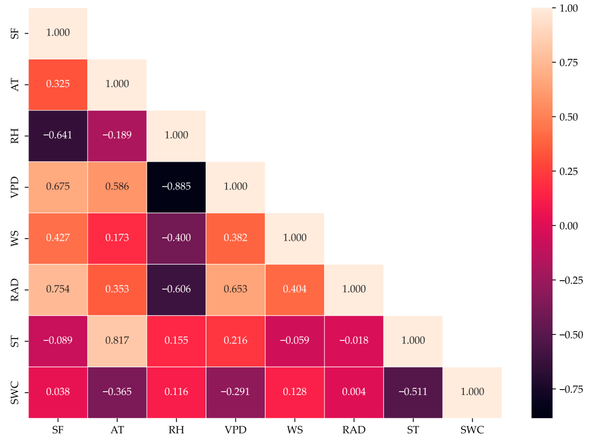
2.4. Correlation Analysis

To evaluate the relationship between the sap flow velocity and the seven environmental parameters, AT, RH, VPD, RAD, WS, ST, and SWC made up this list of variables. To investigate the effect of environmental factors on the sap flow velocity, a Pearson correlation analysis was performed between the sap flow velocity and each environmental factor [35]. When the absolute value of the correlation coefficient is less than 0.3, it indicates that there is a weak correlation between the variables. When the absolute value of the correlation coefficient is between 0.3 and 0.6, it indicates that there is a more significant correlation between the variables. When the absolute value of the correlation coefficient is greater than 0.6, there is a strong and significant correlation between the variables.

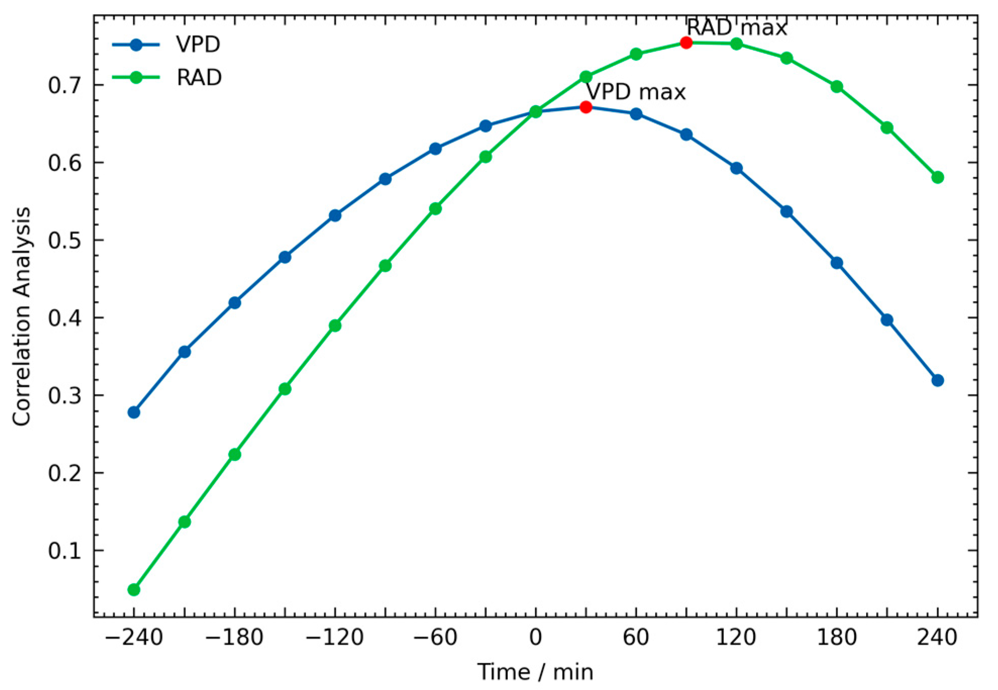
2.5. Time-Lag Effect Analysis

It was found that transient environmental factors were significantly correlated with trunk sap flow, but there was a time-lag effect between them [36]. However, many previous studies analyzed simultaneous data from both, leading to errors in the prediction models of sap flow based on environmental factors. To address this issue, we employed the dislocation contrast method to analyze the time-lag effect between sap flow and environment factors [28]. We combined sap flow velocities and environmental parameters into data columns based on time periods and integrated the data for each driving factor with sap flow velocity data into 30-min periods. Using this method, the data was moved one by one. We then performed a correlation analysis on the combined data, identifying the period with the highest correlation value as the time-lag value of the driver.

2.6. AI Algorithms

KNN is a non-parametric method that does not require defining or training parameters between the independent and dependent variables [37]. This method refers to the K training samples that are closest to the test samples, and the regression values are predicted by the similarity of the characteristics of the training samples to the test values [38]. The number of neighbors, weights of points, distances, and p-parameters associated with the Minkowski function are the factors considered when optimizing the model [39]. The number of neighbors K indicates how many groups the dependent variable is divided into. K is the key conditioning parameter in KNN regression [40]. The selection of the K value is very important for the accurate analysis of sap flow velocity data using KNN. The weights of the points are defined in two modes according to the distances in the model: uniform and weighted. The prediction accuracy of the KNN method is very sensitive to the choice of distance metric [41] and the distance judgment metrics include four types: Euclidean distance, Marxian distance, most similar nearest neighbor, and distance metric based on the nearest neighbor matrix [37].
RF is an integrated learning approach developed by Breiman [42]. The learning task of RF is done by constructing and combining multiple classifiers. Furthermore, the model simply contains two parameters (the number of variables in a random subset at each node and the number of trees in the forest). As a result, RF is simple to construct [43]. Integrated learning methods are broadly classified into two categories: boosting methods and bagging methods [44]. RF is a variant of the bagging method, which is similar to decision trees in that bootstrap samples are extracted to build multiple trees; the difference is that each tree in RF is grown with a random subset of predictors [45].
BPNN is a method proposed by Rumelhart and McClelland in 1986 that is based on the idea that multilayer feedforward neural networks achieve self-organization, self-adaptation, and self-learning to deal with nonlinear problems through the process of error back propagation [46,47]. The computational process of the BP neural network includes forward and backward computation. Firstly, neurons receive information from the outside world in the input layer of the forward propagation process of BP neural networks. Then, the information is processed layer by layer into the output layer under various parameters (weights, deviation values) and activation functions. The algorithm initiates the backpropagation process when the error between the actual output and the target output exceeds the acceptable error range. In the next step, the algorithm will correct the weights of each layer according to the gradient descent method. At the same time, the error is propagated to the hidden layer and the input layer. The weights between the layers are continuously adjusted according to the gradient descent approach. When the output reaches the expected result or a predefined number of learning iterations, the training is ended and the BP neural network completes the learning process [48]. The principles and formulas of neural networks can be found in [49]. The number of hidden layers and the number of neurons in each layer of the BP neural network are set according to the specific situation.
Recurrent neural networks (RNN) are designed to deal with serial dependencies [50], so they can extract the temporal information in the data. In time series problems, RNN is commonly used [51]. Although RNN models have the ability to efficiently process nonlinear time series, they often suffer from gradient vanishing and explosion problems due to the difficulty of solving the long-term dependency of time series data [51]. LSTM aims to solve the long-term dependency problem encountered by traditional RNNs when dealing with long sequences, and efficiently captures the contextual information in the sequences through the introduction of a gating mechanism [52]. The LSTM unit is the basic building block of an LSTM network with forgetting gate, input gate, and output gate [53]. The forgetting gate determines which information from the memory state of the previous time step needs to be forgotten, the input gate controls the input of new information, and the output gate controls the output of the current time step. These gates adjust the flow of information by means of learnable weights, thus enabling the modeling of information at different time steps in the sequence. At each time step, the LSTM unit receives the input data and the hidden state of the previous time step. First, the values of the forgetting gate, input gate, and output gate are calculated based on the input data and the hidden state of the previous time step. Then, the values of the gates are utilized to control the update of the memorized state and the hidden state at the current time step. This gating mechanism allows the LSTM to efficiently capture long-term dependencies and avoids the gradient vanishing and gradient explosion problems.

2.7. Data Acquisition, Sample Segmentation, Data Processing, and Model Tuning

The study used data from three standard Magnolia trees collected from March to September in 2021 and 2022 as samples for the model. The dataset includes sap flow, atmospheric, and soil data. To analyze and compare the changes in sap flow velocity of Magnolia trees at different time periods, we selected a sunny day of each month as a standard day. Five sap flow indicators were counted on the standard day, i.e., sap flow initiation time, peak time, peak value, mean value, and trough time. To minimize the impact of precipitation on sap flow, data from rainy days were excluded. The entire dataset (n = 24,907) was divided into 80% training set and 20% testing set. To validate the effectiveness of the VMI theory in sap flow monitoring, we added a target tree. While the environmental factors and sap flow velocity of the target tree were monitored, the sap data was not input into the training model. The monitoring of the target tree was carried out from 10–20 August 2023. Our goal was to input the environmental factor data of the target tree into the model and obtain the estimated sap flow velocity for that time period. The aim was to verify whether a trained AI algorithm can estimate the sap flow velocity at an acceptable level with only environmental factor data. The survival rate of large-sized tree transplantation is a key factor affecting the efficient greening of urban gardens, especially for Shanghai, where the city flower is Magnolia. Therefore, we chose four large-diameter magnolia trees with good growth and development that were aged around 15 years in the study area as the study subjects (Table 1).
We used the R package TREX.R (v1.0.0) on the R platform (v 4.1.2) for data preprocessing [54]. The processing employed the functions presented in Table 2.
After processing with the TREX.R package, we obtained the data in Excel format corresponding to the sap flow and environmental factors. Subsequently, on the Spyder platform (v5.3.3), we used the Sklearn library (v0.22.1) for Python (v3.9.13) to build a sap flow velocity fitting model based on KNN and RF methods [55]. The parameter values of the model with the highest fitting accuracy were selected by using the grid search method. Prediction models for BPNN and LSTM were built using the PyTorch library (v1.3) [56]. The neural network models utilized algorithms from the Optuna library (v3.0.3) for parameter tuning [57]. Ultimately, the most effective deep learning neural network structure was selected.

2.8. Model Verification

The input variables were normalized to mitigate the impact of differences in the magnitude scale between the data. To mitigate the influence of data differences, we conducted a normalization process on the input variables (i.e., environmental variables). Equation (3) was used for the specific treatment [56]:
x n o r m = x x m i n x m a x x m i n
where x n o r m , x , x m i n , and x m a x represent the normalized, original, minimum, and maximum values of each environmental factor in the training data, respectively.
In order to assess the accuracy of the tree sap flow estimation model, we employed metrics such as the mean absolute error (MAE), mean squared error (MSE), root mean squared error (RMSE), and coefficient of determination (R2). The calculation methods for MAE, MSE, RMSE, and R2 are detailed in Equations (4)–(7), respectively:
M A E = 1 n × i = 1 n y i y ^ i
M S E = i = 1 n y i y ^ i 2 n
R M S E = i = 1 n y i y ^ i 2 n
R 2 = 1 i = 1 n y i y ^ i 2 i = 1 n y i y ̄ i 2
where n , y i , and y ^ i represent the number of data sets, measured values, and estimated values, respectively.

3. Results

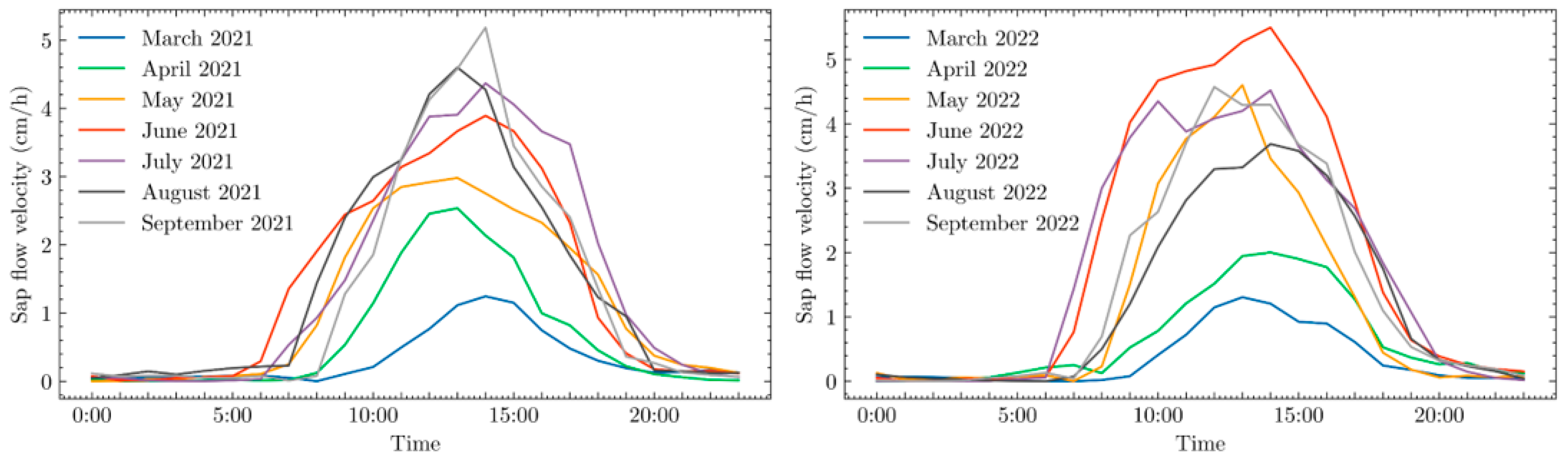
3.1. Monthly Variation Pattern and Comparison of Sap Flow Density

The flow velocity of the Magnolia sap exhibits a unimodal daily variation, rapidly declining after reaching the peak until it reaches the trough (Figure 1). The average daily flow velocity ranged from 0.3294 to 1.9780 cm/h. The sap flow was initiated daily from 7:00 to 9:00, reached a peak between 1.24 and 5.49 cm/h from 13:00 to 14:30, declined rapidly after reaching the peak, and reached a trough within 17:30 to 19:30. The sap flow velocity floated in the range of 0–0.7619 cm/h during the night until the sap flow restarts the next day. In terms of time to peak, there was no significant difference in the time to peak sap flow velocity over the months. In terms of peak and daily average sap flow velocity, the peak of the sap flow velocity of Magnolia was the largest in June, with values of 5.18 and 5.49 cm/h in both years, and the smallest in March, with values of 1.21 and 1.31 cm/h. The maximum and average flow velocity in Magnolia during the experiment, ranked in descending order for different months in 2021 and 2022, are as follows: June > May > July > September > August > March > April; June > July > September > May > August > April > March (Table 3).

3.2. Correlation and Time-Lag Analysis of Factors Influencing Sap Flow Velocity

After analyzing the time-lag effect using the dislocation contras method, the correlation between VPD, RAD, and sap flow velocity reached its maximum at a lag of 30 min and 90 min (Figure 2). However, Ta, WS, and RH did not exhibit significant time-lag effects. The correlation of VPD increased from an initial value of 0.671 to 0.675, while the correlation of RAD rose from 0.670 to 0.754. Since the threshold for the transition of environmental factors’ correlation with sap flow velocity was set at an absolute value of 0.3, the ST and SWC indicators were excluded when constructing the sap flow velocity estimation model (Figure 3). The model incorporated the time-lag effect of RAD and VPD, as well as WS, AT, and RH at corresponding normal moments during the construction of the sap flow velocity estimation model.

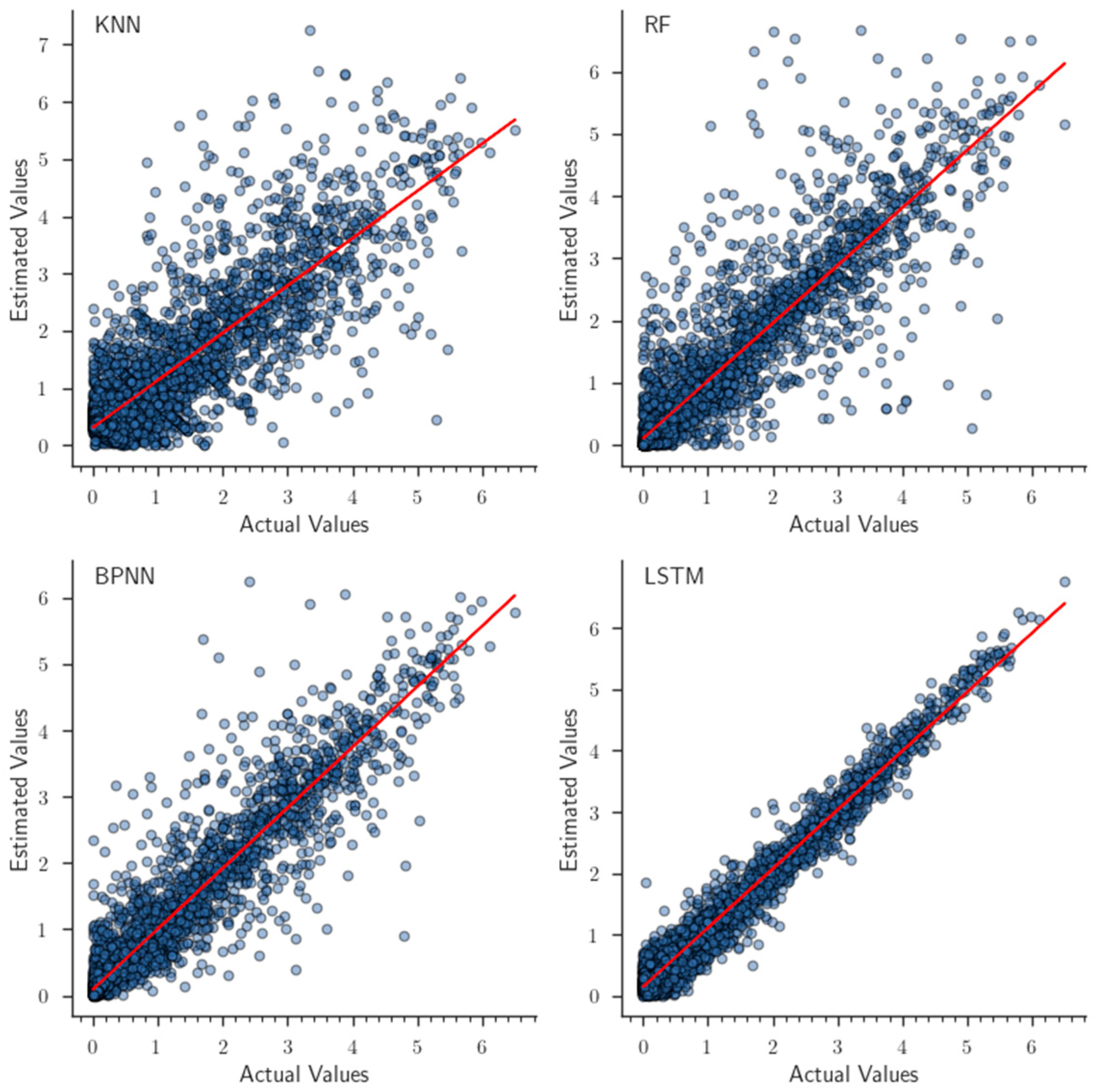
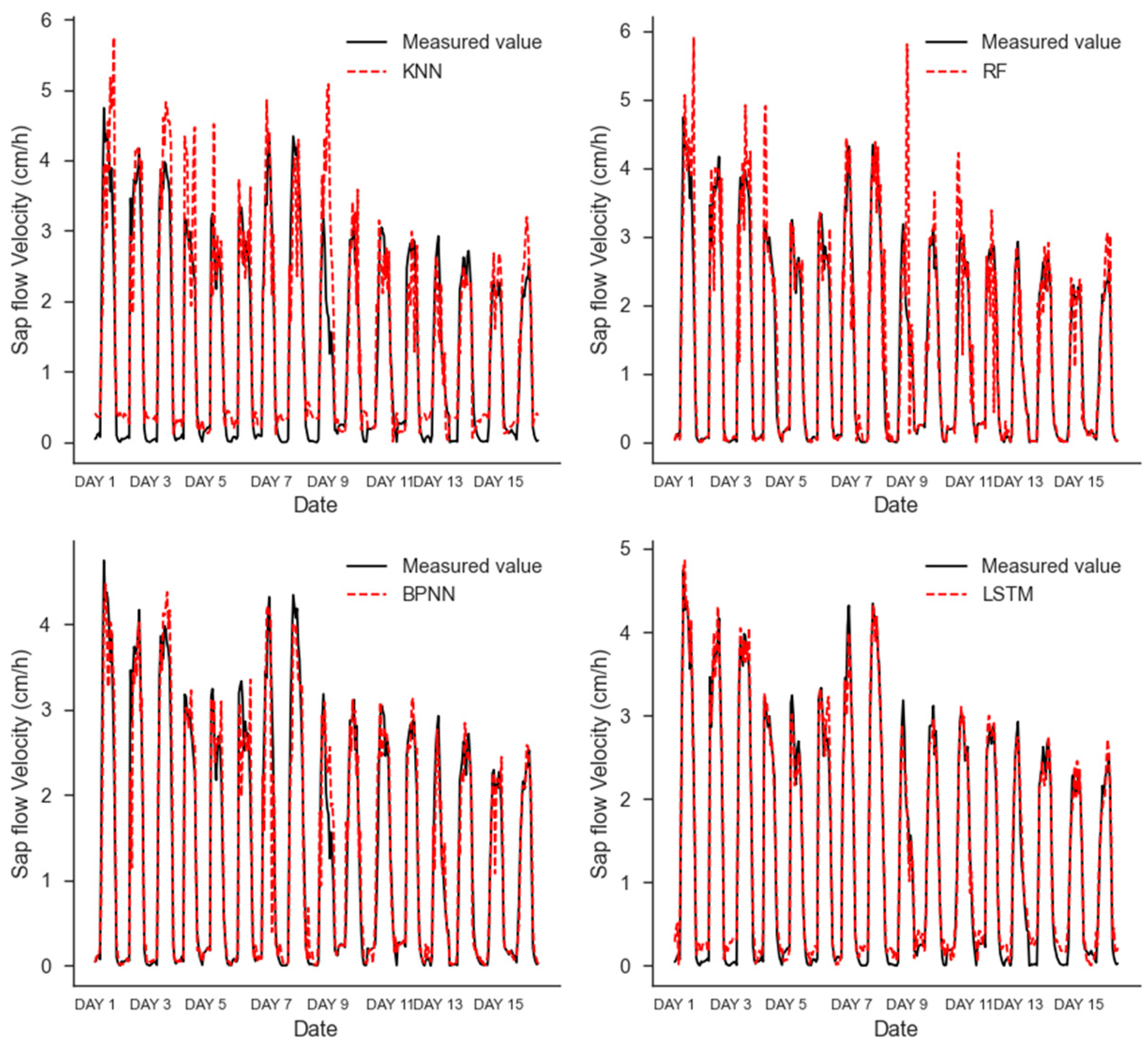
3.3. Performance Comparison of AI Sap Flow Velocity Estimation Models

This study conducted a comprehensive comparison of the performance and fitting ability of four AI algorithms—KNN, RF, BPNN, and LSTM—for estimating sap flow velocity. The results showed that the R² values of the four models ranked as LSTM > BPNN > RF > KNN, indicating that the LSTM model achieved the highest estimation accuracy among the four models (Table 4). For the specific values, the R² values of KNN, RF, BPNN, and LSTM models were 0.688, 0.797, 0.889, and 0.957, respectively. The corresponding MAE values were 0.456, 0.254, 0.203, and 0.189, while the MSE values were 0.434, 0.282, 0.155, and 0.059, and the RMSE values were 0.658, 0.531, 0.394, and 0.243. According to the results from the validation set, all four models demonstrated satisfactory estimation accuracy, with the LSTM model being particularly notable.
The trends in the estimated values for the four models were highly consistent with the trends in the actual sap flow velocity values (Figure 4). However, compared with the other models, the estimation of the KNN model in the range of 0–2 cm/h sap flow velocity showed obvious bias; especially in the sap flow velocity estimation results beyond this range, a considerable number of low actual values and high estimated values appear. The RF model also had a certain degree of bias in the estimation of low sap flow velocity of 0–2 cm/h, although the sap flow velocity in the range beyond 2 cm/h is estimated with overall higher accuracy. Although the overall accuracy was higher in the estimation of sap flow velocity over 2 cm/h, there is still a phenomenon of low actual value and high estimated value similar to that of the KNN model. In contrast, the fitted graphs of BPNN were closer to the ideal y = x straight line, which significantly reduced the appearance of outliers, although a few outliers still existed. The LSTM model exhibited exceptional estimation capabilities throughout the entire dataset. Furthermore, the simulation curves of the LSTM model are notably smoother than other models, particularly at higher sap flow velocity, and it is largely free of outliers. In the range of low sap flow velocity, it is important to note that the LSTM model’s estimates exhibit slight deviations from the actual values. However, overall, it outperforms the other models.

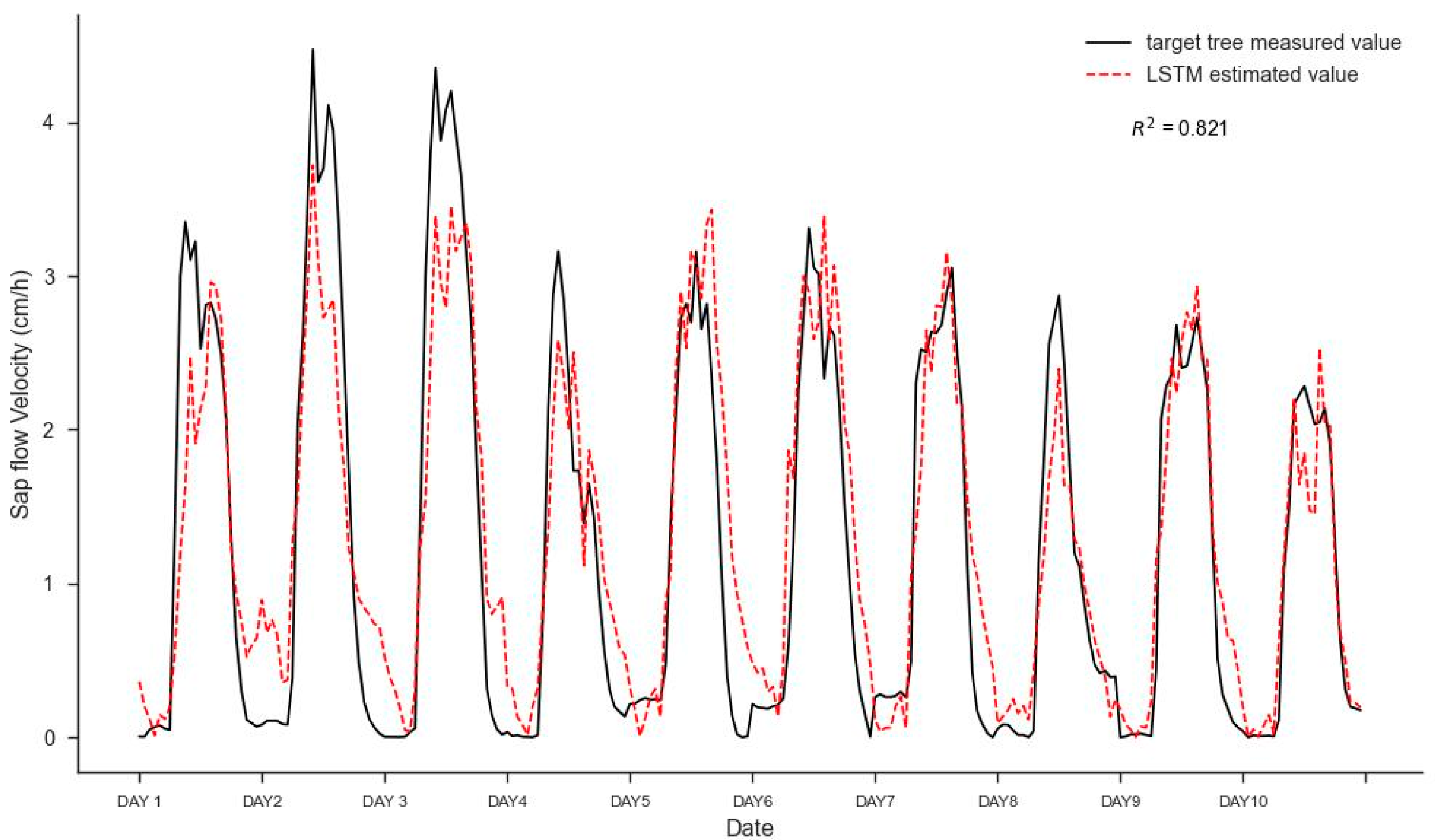
3.4. Analysis of Results for Target Tree Accuracy Validation

The estimations of sap flow velocity by the four models were compared with the actual values (Figure 5). Consistent with the performance indicators previously presented by each model, the LSTM model demonstrated a strong fitting capability. Based on the results after inputting the environmental factor data of the target tree into the LSTM model, we found that the LSTM model tended to be conservative in estimating the peak values of sap flow velocity of the target tree, while it tended to be aggressive in estimating the valley values (Figure 6). This phenomenon was particularly evident during the time when there were high peaks and low valleys in sap flow velocity. Although the LSTM model showed some deviations in these cases, the estimated results achieved an R2 of 0.821. In the ten-day dataset, the total flow volume was 297.418 cm, while the estimated flow volume was 311.985 cm, resulting in an error of 14.567 cm, with an error rate of only 4.89%. Overall, the estimation performance of the LSTM model was satisfactory.

4. Discussion

In this study, we observed a close relationship between sap flow velocity and environmental factors. AT, RH, VPD, WS, and RAD are the environmental factors that have the most significant impact on the sap flow velocity of Magnolia. In our study, RAD and VPD play a crucial role in sap flow. High temperatures, in particular, lead to a rise in VPD, which, in turn, increases leaf transpiration (provided stomata do not close) [58]. WS can change the air conditions and leaf humidity near the canopy [59]. The sap flow velocity of Magnolia was greatly influenced by external environmental factors and exhibits noticeable time-lag effects. It is worth noting that the sap flow lags behind VPD by 30 min and behind RAD by 90 min, while AT, WS, and RH do not show a significant time-lag effect. The sap flow usually lags behind RAD, but precedes VPD [60]. However, in some studies, the sap flow lags behind VPD and RAD, which is consistent with our research results [61]. Therefore, in the modeling process, we need to consider not only the selection of environmental features, but also the time-lag response of sap flow to these environmental features to improve the accuracy of the model.
AI algorithms play a central role in VMI measurements. In this study, the KNN algorithm was used to estimate the sap flow velocity, but its R2 was only 0.688. Although KNN can effectively handle nonlinear problems in certain cases, its performance may not be satisfactory for time series data with complex periodic patterns [62]. This is mainly because the KNN model ignores the temporality of data; thus, it is unable to consider the temporal relationships and intervals between data points [63]. This limits its ability to capture cyclical changes. While most sap flow studies adopt the RF algorithm, which achieved acceptable accuracy in this study with an R2 of 0.797, its predictive ability is limited when dealing with time series data, such as sap flow. This is because the decision trees in RF do not explicitly consider the temporal characteristics of the data, and mainly focus on the static relationship between inputs and outputs rather than dynamic processes [25,64]. Therefore, RF struggles to capture relevant features when dealing with obvious cyclical variations. In contrast, the BPNN algorithm achieved an R2 of 0.889 in the prediction results. However, similarly, BPNN also does not consider the temporal characteristics of the data. Although BPNN demonstrates satisfactory predictive performance in certain cases, it can easily get stuck in local minima in time series data with complex cyclical variations, limiting its predictive ability [65,66]. Unlike the aforementioned three algorithms, the LSTM networks are neural network models specifically designed to handle time series data. Through its memory mechanism, LSTM can capture long-term dependencies in the data and is particularly good at dealing with time series data with cyclical variations [30]. In predicting sap flow data, LSTM demonstrated the ability to understand and predict daily and yearly cyclical variations. Therefore, compared to other models, LSTM often exhibits superior predictive performance, with an R2 as high as 0.957.
VMI integrates real measurement instrument results with computer algorithms to simulate the measuring behavior of another measurement instrument. Based on the concept of VMI, we regard devices that monitor environmental factors (such as small weather stations, drones, and remote sensing satellites) as measurement instruments of VMI. With the AI algorithm based on environmental factors, we can use AI algorithms to replace the traditional thermal technology for obtaining sap flow velocity data. Due to cost limitations, we only validated one VMI case, which is the target tree, using virtual measurement methods. In this assumption, we input the training data of standard trees into the AI model, and the actual measurement data of the target tree is not included in the training set of the model. After the training of the AI model, we chose the LSTM algorithm with the highest accuracy to simulate the sap flow velocity of the target trees and achieved satisfactory simulation results, with an R2 of 0.821 and an error rate of only 4.89%.
However, the limitation of the amount of input data samples is often an important factor affecting the accuracy of AI algorithms [67]. Obtaining ground sap flow monitoring data is usually complex and costly. Nowadays, there are various types of sensors available on the market for monitoring meteorological and soil factors, with a wide price range from economical options to high-end products.
In the current field of scientific research, access to reliable and rich data is crucial for the development of powerful AI algorithms. It is in this context that SAPFLUXNET was born [68]. SAPFLUXNET is a global database that collects sap flow data, environmental data, and various levels of metadata from researchers around the world [69]. It is of great value to explore how to use the SAPFLUXNET database to train sap flow AI algorithms for different tree species and achieve high-precision estimation [70]. For example, based on the SAPFLUXNET database, Li et al. [30] used various AI algorithms, such as MLP, RF, SVR, BPNN, LSTM, CNN-LSTM, and CGRU, among which the R2 of the CGRU algorithm reached 0.948, higher than the LSTM algorithm. Although the accuracy of the LSTM algorithm in this study exceeds the above case, the different dataset size or tree species factors may be the reasons for this difference. It is worth noting that, although the accuracy of certain AI algorithms may vary in different studies, algorithms that incorporate memory mechanisms generally perform better [30]. In addition to using public data, using synthetic data (SD) is also a new approach to address the shortage of data [71]. SD simulates the statistical characteristics of real data and can be synthesized from existing datasets through generative adversarial networks (GANs) [72]. In some related studies, the use of GAN methods to synthesize SD data and use them for neural network algorithm prediction of sap flow achieved an R2 of up to 0.92 [73]. These two data acquisition methods significantly reduce data collection costs while providing many samples for AI algorithm training.
In addition to ground environmental factor data, remote sensing technology is also a feasible method [74]. To some extent, large-scale estimation based on remote sensing technology is the application of VMI theory. By using surface temperature recorded by drones as input indicators for a RF model, the sap flow prediction of this model achieved an R2 of 0.87 compared to ground-measured sap flux [75]. Furthermore, by combining Sentinel-2 images, ground survey data, and local meteorological data, training RF algorithm showed a training R2 ranging from 0.57 to 0.80 in cross-validation at the measurement site [76]. This indicates that, by integrating field data and remote sensing data, scale enhancement can be achieved at a larger spatial scale, enabling estimation of transpiration at plot, or even landscape, scales using AI modeling algorithms.
As emphasized, VMI is a measurement process that combines instrument measurement results with AI algorithms. In fact, the instrument measurement results themselves are the data. To achieve excellent simulation results of sap flow for different tree species in different scenarios using AI algorithms, a large dataset is needed to support algorithm training. However, this study is limited to Magnolia in urban green spaces, and the available data is relatively limited. Furthermore, with the development of deep learning models, an increasing number of AI algorithms are emerging. Further validation is needed in future research to determine which AI algorithms are most suitable for forest transpiration estimation.

5. Conclusions

In this study, we introduced the concept of VMI theory with the aim of solving the challenge of sap flow measurement by indirect measurement. By analyzing the sap flow data of Magnolia trees from March to September in 2021 and 2022, we input the environmental factors, considering the time-lag effect, into four AI algorithms. We compared and analyzed the prediction results of KNN, RF, BPNN, and LSTM models. The results showed that there was no significant correlation between Magnolia sap flow velocity and SWC and ST. However, there were significant correlations between VPD, AT, RAD, RH, and WS and sap flow velocity. The lag times of sap flow on RAD and VPD were 90 and 30 min, respectively. After comparing and analyzing the models, we found that the LSTM model showed the best performance. On the test set samples, the R², MAE, MSE, and RMSE of the LSTM model reached 0.957, 0.189, 0.059, and 0.243, respectively. By inputting the environmental data of the target logs from 10–20 August 2023 into the LSTM model, we obtained a value of R² of 0.821, with a simulated sap flow value error of only 4.89%. Therefore, the LSTM model constructed based on the TDP method provides a feasible means of indirect measurement, i.e., by inputting environmental factors and thus obtaining sap flow estimates, which has some practical application value.

Author Contributions

D.Z., B.Z., Z.F., L.Z. and Z.W. conceived and designed the study; R.F. and B.Z. collected the data; B.Z. and M.Z. processed the data; B.Z. and M.Z. performed the model fitting; B.Z., D.Z. and Z.F. supported data analysis; and B.Z., Z.W. wrote the main manuscript. All authors have read and agreed to the published version of the manuscript.

Funding

This research was funded by the Key R&D Program of Shanghai Science and Technology Commission “Intelligent Technologies and Demonstration of High-quality Landscape Greening for Urban Challenging Sites based on Biodiversity” (Project No. 22dz1202200), the National Key R&D Program of China “Construction of Multi-functional Coupled Network and Ecological Restoration Technology for Typical Urban Corridors” (Project No. 2022YFC3802604), the Natural Science Foundation of Beijing (8232038, 8234065) and the Key Research and Development Projects of Ningxia Hui Autonomous Region (2023BEG02050).

Data Availability Statement

Not applicable.

Acknowledgments

The authors sincerely thank the editors and the anonymous reviewers for their constructive feedback.

Conflicts of Interest

The authors declare no conflict of interest.

References

  1. Bauer, E.; Kohavi, R. An Empirical Comparison of Voting Classification Algorithms: Bagging, Boosting, and Variants. Mach. Learn. 1999, 36, 105–139. [Google Scholar] [CrossRef]
  2. Leghari, S.J.; Wahocho, N.A.; Laghari, G.M.; Hafeez Laghari, A.; Mustafa Bhabhan, G.; Hussain Talpur, K.; Bhutto, T.A.; Wahocho, S.A.; Lashari, A.A. Role of nitrogen for plant growth and development: A review. Adv. Environ. Biol. 2016, 10, 209–219. [Google Scholar]
  3. Wang, H.; Inukai, Y.; Yamauchi, A. Root Development and Nutrient Uptake. Crit. Rev. Plant Sci. 2006, 25, 279–301. [Google Scholar] [CrossRef]
  4. Karthika, K.S.; Rashmi, I.; Parvathi, M.S. Biological Functions, Uptake and Transport of Essential Nutrients in Relation to Plant Growth. In Plant Nutrients and Abiotic Stress Tolerance; Hasanuzzaman, M., Fujita, M., Oku, H., Nahar, K., Hawrylak-Nowak, B., Eds.; Springer: Singapore, 2018; pp. 1–49. ISBN 978-981-10-9044-8. [Google Scholar]
  5. Granier, A.; Bobay, V.; Gash, J.H.C.; Gelpe, J.; Saugier, B.; Shuttleworth, W.J. Vapour flux density and transpiration rate comparisons in a stand of Maritime pine (Pinus pinaster Ait.) in Les Landes forest. Agric. For. Meteorol. 1990, 51, 309–319. [Google Scholar] [CrossRef]
  6. Lapitan, R.L.; Parton, W.J. Seasonal variabilities in the distribution of the microclimatic factors and evapotranspiration in a shortgrass steppe. Agric. For. Meteorol. 1996, 79, 113–130. [Google Scholar] [CrossRef]
  7. Guédon, Y.; Costes, E.; Rakocevic, M. Modulation of the yerba-mate metamer production phenology by the cultivation system and the climatic factors. Ecol. Model. 2018, 384, 188–197. [Google Scholar] [CrossRef]
  8. Oberbauer, S.F.; Strain, B.R.; Riechers, G.H. Field water relations of a wet-tropical forest tree species, Pentaclethra macroloba (Mimosaceae). Oecologia 1987, 71, 369–374. [Google Scholar] [CrossRef]
  9. Zhu, Y.; Li, D.; Fan, J.; Zhang, H.; Eichhorn, M.P.; Wang, X.; Yun, T. A reinterpretation of the gap fraction of tree crowns from the perspectives of computer graphics and porous media theory. Front. Plant Sci. 2023, 14, 1109443. [Google Scholar] [CrossRef]
  10. Marshall, D.C. Measurement of Sap Flow in Conifers by Heat Transport. Plant Physiol. 1958, 33, 385–396. [Google Scholar] [CrossRef]
  11. Granier, A. A new method of sap flow measurement in tree stems. Ann. For. Sci. 1985, 42, 193–200. [Google Scholar] [CrossRef]
  12. Liu, Z.-Q.; Wang, Y.-S.; Zhang, H.; Jia, G.-D. Characteristics and processes of reverse sap flow of Platycladus orientalis based on stable isotope technique and heat ratio method. Ying Yong Sheng Tai Xue Bao 2020, 31, 1817–1826. [Google Scholar] [CrossRef]
  13. Du, F.; Liang, Z.S.; Shan, L.; Shan, C. Evapotransp iration measurements of community using weighting metho. Acta Bot. Boreali-Occident. Sin. 2003, 23, 1411–1415. [Google Scholar]
  14. Biao, Z.; Dongmei, Z.; Lang, Z.; Zhongke, F.; Linhao, S. Development of Trunk Sap Flow Monitoring System. J. Agric. Sci. Technol. 2022, 24, 121–129. [Google Scholar]
  15. Bohua, S.; Ge, G.; Shan, G.; Linlin, S.; Bingxue, L. Overview of the methods for sap flow measurement of standing tree based on thermal technology. J. Zhejiang A F Univ. 2022, 39, 456–464. [Google Scholar] [CrossRef]
  16. Pasqualotto, G.; Carraro, V.; Menardi, R.; Anfodillo, T. Calibration of Granier-Type (TDP) Sap Flow Probes by a High Precision Electronic Potometer. Sensors 2019, 19, 2419. [Google Scholar] [CrossRef]
  17. Wang, Z.; Shen, Y.-J.; Zhang, X.; Zhao, Y.; Schmullius, C. Processing Point Clouds Using Simulated Physical Processes as Replacements of Conventional Mathematically Based Procedures: A Theoretical Virtual Measurement for Stem Volume. Remote Sens. 2021, 13, 4627. [Google Scholar] [CrossRef]
  18. Chang, X.; Zhao, W.; He, Z. Radial pattern of sap flow and response to microclimate and soil moisture in Qinghai spruce (Picea crassifolia) in the upper Heihe River Basin of arid northwestern China. Agric. For. Meteorol. 2014, 187, 14–21. [Google Scholar] [CrossRef]
  19. Liu, W.; Wei, T.; Zhu, Q. Growing season sap flow of Populus hopeiensis and Pinus tabulaeformis in the semi-arid Loess Plateau, China. J. Zhejiang A&F Univ. 2018, 35, 1045–1053. [Google Scholar]
  20. Ruas, K.F.; Baroni, D.F.; de Souza, G.A.R.; Bernado, W.d.P.; Paixão, J.S.; dos Santos, G.M.; Filho, J.A.M.; de Abreu, D.P.; de Sousa, E.F.; Rakocevic, M.; et al. A Carica papaya L. genotype with low leaf chlorophyll concentration copes successfully with soil water stress in the field. Sci. Hortic. 2022, 293, 110722. [Google Scholar] [CrossRef]
  21. Čermák, J.; Kučera, J.; Nadezhdina, N. Sap flow measurements with some thermodynamic methods, flow integration within trees and scaling up from sample trees to entire forest stands. Trees 2004, 18, 529–546. [Google Scholar] [CrossRef]
  22. Liu, Z.; Peng, C.; Work, T.; Candau, J.-N.; DesRochers, A.; Kneeshaw, D. Application of machine-learning methods in forest ecology: Recent progress and future challenges. Environ. Rev. 2018, 26, 339–350. [Google Scholar] [CrossRef]
  23. Li, X.; Wang, X.; Gao, Y.; Wu, J.; Cheng, R.; Ren, D.; Bao, Q.; Yun, T.; Wu, Z.; Xie, G.; et al. Comparison of Different Important Predictors and Models for Estimating Large-Scale Biomass of Rubber Plantations in Hainan Island, China. Remote Sens. 2023, 15, 3447. [Google Scholar] [CrossRef]
  24. Fan, J.; Zheng, J.; Wu, L.; Zhang, F. Estimation of daily maize transpiration using support vector machines, extreme gradient boosting, artificial and deep neural networks models. Agric. Water Manag. 2021, 245, 106547. [Google Scholar] [CrossRef]
  25. Peng, X.; Hu, X.; Chen, D.; Zhou, Z.; Guo, Y.; Deng, X.; Zhang, X.; Yu, T. Prediction of Grape Sap Flow in a Greenhouse Based on Random Forest and Partial Least Squares Models. Water 2021, 13, 3078. [Google Scholar] [CrossRef]
  26. Liu, X.; Kang, S.; Li, F. Simulation of artificial neural network model for trunk sap flow of Pyrus pyrifolia and its comparison with multiple-linear regression. Agric. Water Manag. 2009, 96, 939–945. [Google Scholar] [CrossRef]
  27. Li, Y.; Chen, Q.; He, K.; Wang, Z. The accuracy improvement of sap flow prediction in Picea crassifolia Kom. based on the back-propagation neural network model. Hydrol. Process. 2022, 36, e14490. [Google Scholar] [CrossRef]
  28. Tu, J.; Wei, X.; Huang, B.; Fan, H.; Jian, M.; Li, W. Improvement of sap flow estimation by including phenological index and time-lag effect in back-propagation neural network models. Agric. For. Meteorol. 2019, 276–277, 107608. [Google Scholar] [CrossRef]
  29. Nalevanková, P.; Fleischer, P.; Mukarram, M.; Sitková, Z.; Střelcová, K. Comparative Assessment of Sap Flow Modeling Techniques in European Beech Trees: Can Linear Models Compete with Random Forest, Extreme Gradient Boosting, and Neural Networks? Water 2023, 15, 2525. [Google Scholar] [CrossRef]
  30. Li, Y.; Ye, J.; Xu, D.; Zhou, G.; Feng, H. Prediction of sap flow with historical environmental factors based on deep learning technology. Comput. Electron. Agric. 2022, 202, 107400. [Google Scholar] [CrossRef]
  31. Lu, P.; Urban, L.; Zhao, P. Granier’s thermal dissipation probe (TDP) method for measuring sap flow in trees: Theory and practice. Acta Bot. Sin. 2004, 46, 631–646. [Google Scholar]
  32. Rabbel, I.; Diekkrüger, B.; Voigt, H.; Neuwirth, B. Comparing ∆Tmax Determination Approaches for Granier-Based Sapflow Estimations. Sensors 2016, 16, 2042. [Google Scholar] [CrossRef] [PubMed]
  33. Oishi, A.C.; Hawthorne, D.A.; Oren, R. Baseliner: An open-source, interactive tool for processing sap flux data from thermal dissipation probes. SoftwareX 2016, 5, 139–143. [Google Scholar] [CrossRef]
  34. Granier, A. Evaluation of Transpiration in a Douglas-Fir Stand by Means of Sap Flow Measurements. Tree Physiol. 1987, 3, 309–320. [Google Scholar] [CrossRef]
  35. Cleophas, T.J.; Zwinderman, A.H. Bayesian Pearson Correlation Analysis. In Modern Bayesian Statistics in Clinical Research; Cleophas, T.J., Zwinderman, A.H., Eds.; Springer International Publishing: Cham, Switzerland, 2018; pp. 111–118. ISBN 978-3-319-92747-3. [Google Scholar]
  36. Zhang, R.; Xu, X.; Liu, M.; Zhang, Y.; Xu, C.; Yi, R.; Luo, W.; Soulsby, C. Hysteresis in sap flow and its controlling mechanisms for a deciduous broad-leaved tree species in a humid karst region. Sci. China Earth Sci. 2019, 62, 1744–1755. [Google Scholar] [CrossRef]
  37. Chirici, G.; Barbati, A.; Corona, P.; Marchetti, M.; Travaglini, D.; Maselli, F.; Bertini, R. Non-parametric and parametric methods using satellite images for estimating growing stock volume in alpine and Mediterranean forest ecosystems. Remote Sens. Environ. 2008, 112, 2686–2700. [Google Scholar] [CrossRef]
  38. Franco-Lopez, H.; Ek, A.R.; Bauer, M.E. Estimation and mapping of forest stand density, volume, and cover type using the k-nearest neighbors method. Remote Sens. Environ. 2001, 77, 251–274. [Google Scholar] [CrossRef]
  39. Keramat-Jahromi, M.; Mohtasebi, S.S.; Mousazadeh, H.; Ghasemi-Varnamkhasti, M.; Rahimi-Movassagh, M. Real-time moisture ratio study of drying date fruit chips based on on-line image attributes using kNN and random forest regression methods. Measurement 2021, 172, 108899. [Google Scholar] [CrossRef]
  40. Qian, Y.; Zhou, W.; Yan, J.; Li, W.; Han, L. Comparing Machine Learning Classifiers for Object-Based Land Cover Classification Using Very High Resolution Imagery. Remote Sens. 2015, 7, 153–168. [Google Scholar] [CrossRef]
  41. Cosenza, D.N.; Korhonen, L.; Maltamo, M.; Packalen, P.; Strunk, J.L.; Næsset, E.; Gobakken, T.; Soares, P.; Tomé, M. Comparison of linear regression, k-nearest neighbour and random forest methods in airborne laser-scanning-based prediction of growing stock. For. Int. J. For. Res. 2021, 94, 311–323. [Google Scholar] [CrossRef]
  42. Breiman, L. Random Forests. Mach. Learn. 2001, 45, 5–32. [Google Scholar] [CrossRef]
  43. Liaw, A.; Wiener, M. Classification and Regression by RandomForest. R News 2002, 2, 18–22. [Google Scholar]
  44. Wen, L.; Hughes, M. Coastal Wetland Mapping Using Ensemble Learning Algorithms: A Comparative Study of Bagging, Boosting and Stacking Techniques. Remote Sens. 2020, 12, 1683. [Google Scholar] [CrossRef]
  45. Prasad, A.M.; Iverson, L.R.; Liaw, A. Newer Classification and Regression Tree Techniques: Bagging and Random Forests for Ecological Prediction. Ecosystems 2006, 9, 181–199. [Google Scholar] [CrossRef]
  46. Pan, H.; Yang, J.; Shi, Y.; Li, T. BP Neural Network Application Model of Predicting the Apple Hardness. J. Comput. Theor. Nanosci. 2015, 12, 2802–2807. [Google Scholar] [CrossRef]
  47. Rakkiyappan, R.; Velmurugan, G.; Cao, J. Stability analysis of fractional-order complex-valued neural networks with time delays. Chaos Solitons Fractals 2015, 78, 297–316. [Google Scholar] [CrossRef]
  48. Kubat, M. Neural networks: A comprehensive foundation by Simon Haykin, Macmillan, 1994, ISBN 0-02-352781-7. Knowl. Eng. Rev. 1999, 13, 409–412. [Google Scholar] [CrossRef]
  49. Kisi, O. The potential of different ANN techniques in evapotranspiration modelling. Hydrol. Process. 2008, 22, 2449–2460. [Google Scholar] [CrossRef]
  50. Samuel Sajo, O.; Gbenro Oguntunde, P.; Toyin Fasinmirin, J.; Akinnagbe, A.; Akinlabi Olufayo, A.; Ohikhena Agele, S. Modelling the Canopy Conductance of Cocoa Tree Using a Recurrent Neural Network. Am. J. Neural Netw. Appl. 2021, 7, 23. [Google Scholar] [CrossRef]
  51. Shewalkar, A.; Nyavanandi, D.; Ludwig, S.A. Performance Evaluation of Deep Neural Networks Applied to Speech Recognition: RNN, LSTM and GRU. J. Artif. Intell. Soft Comput. Res. 2019, 9, 235–245. [Google Scholar] [CrossRef]
  52. Hochreiter, S.; Schmidhuber, J. Long Short-Term Memory. Neural Comput. 1997, 9, 1735–1780. [Google Scholar] [CrossRef]
  53. Sherstinsky, A. Fundamentals of Recurrent Neural Network (RNN) and Long Short-Term Memory (LSTM) network. Phys. D Nonlinear Phenom. 2020, 404, 132306. [Google Scholar] [CrossRef]
  54. Peters, R.L.; Pappas, C.; Hurley, A.G.; Poyatos, R.; Flo, V.; Zweifel, R.; Goossens, W.; Steppe, K. Assimilate, process and analyse thermal dissipation sap flow data using the TREX r package. Methods Ecol. Evol. 2021, 12, 342–350. [Google Scholar] [CrossRef]
  55. Hutter, F.; Kotthoff, L.; Vanschoren, J. (Eds.) Automated Machine Learning: Methods, Systems, Challenges; The Springer Series on Challenges in Machine Learning; Springer International Publishing: Cham, Switzerland, 2019; ISBN 978-3-030-05317-8. [Google Scholar]
  56. Paszke, A.; Gross, S.; Massa, F.; Lerer, A.; Bradbury, J.; Chanan, G.; Killeen, T.; Lin, Z.; Gimelshein, N.; Antiga, L.; et al. PyTorch: An Imperative Style, High-Performance Deep Learning Library. In Proceedings of the Advances in Neural Information Processing Systems, Vancouver, BC, Canada, 8–14 December 2019; Curran Associates, Inc.: Red Hook, NY, USA, 2019; Volume 32. [Google Scholar]
  57. Akiba, T.; Sano, S.; Yanase, T.; Ohta, T.; Koyama, M. Optuna: A Next-generation Hyperparameter Optimization Framework. In Proceedings of the 25th ACM SIGKDD International Conference on Knowledge Discovery & Data Mining, Anchorage, AK, USA, 4–8 August 2019; ACM: Anchorage, AK, USA, 2019; pp. 2623–2631. [Google Scholar]
  58. Will, R.E.; Wilson, S.M.; Zou, C.B.; Hennessey, T.C. Increased vapor pressure deficit due to higher temperature leads to greater transpiration and faster mortality during drought for tree seedlings common to the forest–grassland ecotone. New Phytol. 2013, 200, 366–374. [Google Scholar] [CrossRef]
  59. Fuchs, M. Infrared measurement of canopy temperature and detection of plant water stress. Theor. Appl. Climatol. 1990, 42, 253–261. [Google Scholar] [CrossRef]
  60. EBSCOhost|52527203|Time Lag Characteristics of Stem Sap Flow of Common Tree Species during Their Growth Season in Beijing Downtown. Available online: https://web.p.ebscohost.com/abstract?direct=true&profile=ehost&scope=site&authtype=crawler&jrnl=10019332&AN=52527203&h=SJVDKyHkMDFqtnizWoHosjH8C9q8pqZncj%2ftcHG%2fhKGNnOr42dl%2bvBYWLdBK3Ll%2bNVcLYVlWkcTUmVN0R1aTPg%3d%3d&crl=c&resultNs=AdminWebAuth&resultLocal=ErrCrlNotAuth&crlhashurl=login.aspx%3fdirect%3dtrue%26profile%3dehost%26scope%3dsite%26authtype%3dcrawler%26jrnl%3d10019332%26AN%3d52527203 (accessed on 25 November 2022).
  61. Yang, J.; Lyu, J.L.; He, Q.Y.; Yan, M.J.; Li, G.Q.; DU, S. Time lag of stem sap flow and its relationships with transpiration characteristics in Quercus liaotungensis and Robina pseudoacacia in the loess hilly region, China. Ying Yong Sheng Tai Xue Bao 2019, 30, 2607–2613. [Google Scholar] [CrossRef]
  62. Martínez, F.; Frías, M.P.; Pérez, M.D.; Rivera, A.J. A methodology for applying k-nearest neighbor to time series forecasting. Artif. Intell. Rev. 2019, 52, 2019–2037. [Google Scholar] [CrossRef]
  63. Ahmed, N.K.; Atiya, A.F.; Gayar, N.E.; El-Shishiny, H. An Empirical Comparison of Machine Learning Models for Time Series Forecasting. Econom. Rev. 2010, 29, 594–621. [Google Scholar] [CrossRef]
  64. Tyralis, H.; Papacharalampous, G. Variable Selection in Time Series Forecasting Using Random Forests. Algorithms 2017, 10, 114. [Google Scholar] [CrossRef]
  65. Wang, L.; Zeng, Y.; Chen, T. Back propagation neural network with adaptive differential evolution algorithm for time series forecasting. Expert Syst. Appl. 2015, 42, 855–863. [Google Scholar] [CrossRef]
  66. Singh, J.; Tripathi, P. Time Series Forecasting Using Back Propagation Neural Network with ADE Algorithm. Int. J. Eng. Tech. Res. 2017, 7, 265026. [Google Scholar]
  67. Adadi, A. A survey on data-efficient algorithms in big data era. J. Big Data 2021, 8, 24. [Google Scholar] [CrossRef]
  68. Poyatos, R.; Granda, V.; Molowny-Horas, R.; Mencuccini, M.; Steppe, K.; Martínez-Vilalta, J. SAPFLUXNET: Towards a global database of sap flow measurements. Tree Physiol. 2016, 36, 1449–1455. [Google Scholar] [CrossRef] [PubMed]
  69. Poyatos, R.; Granda, V.; Flo, V.; Adams, M.A.; Adorján, B.; Aguadé, D.; Aidar, M.P.M.; Allen, S.; Alvarado-Barrientos, M.S.; Anderson-Teixeira, K.J.; et al. Global transpiration data from sap flow measurements: The SAPFLUXNET database. Earth Syst. Sci. Data 2021, 13, 2607–2649. [Google Scholar] [CrossRef]
  70. Poyatos, R.; Flo, V.; Granda, V.; Steppe, K.; Mencuccini, M.; Martínez-Vilalta, J. Using the SAPFLUXNET database to understand transpiration regulation of trees and forests. Acta Hortic. 2020, 1300, 179–186. [Google Scholar] [CrossRef]
  71. Bolón-Canedo, V.; Sánchez-Maroño, N.; Alonso-Betanzos, A. A review of feature selection methods on synthetic data. Knowl. Inf. Syst. 2013, 34, 483–519. [Google Scholar] [CrossRef]
  72. Figueira, A.; Vaz, B. Survey on Synthetic Data Generation, Evaluation Methods and GANs. Mathematics 2022, 10, 2733. [Google Scholar] [CrossRef]
  73. Balasubramanian, H.K.; Thirugnanam, H. Neural Networking to Predict Sap Flow Using AI-Synthesized Relative Meteorological Data. In Proceedings of the 2023 3rd International Conference on Intelligent Technologies (CONIT), Hubli, India, 23–25 June 2023; pp. 1–7. [Google Scholar]
  74. Nagler, P.; Jetton, A.; Fleming, J.; Didan, K.; Glenn, E.; Erker, J.; Morino, K.; Milliken, J.; Gloss, S. Evapotranspiration in a cottonwood (Populus fremontii) restoration plantation estimated by sap flow and remote sensing methods. Agric. For. Meteorol. 2007, 144, 95–110. [Google Scholar] [CrossRef]
  75. Ellsäßer, F.; Röll, A.; Ahongshangbam, J.; Waite, P.-A.; Hendrayanto; Schuldt, B.; Hölscher, D. Predicting Tree Sap Flux and Stomatal Conductance from Drone-Recorded Surface Temperatures in a Mixed Agroforestry System—A Machine Learning Approach. Remote Sens. 2020, 12, 4070. [Google Scholar] [CrossRef]
  76. Tomelleri, E.; Tonon, G. Linking Sap Flow Measurements with Earth Observations. In Proceedings of the 2021 IEEE International Geoscience and Remote Sensing Symposium IGARSS, Brussels, Belgium, 11–16 July 2021; pp. 6881–6884. [Google Scholar]
Figure 1. Sap flow velocity line graph for each month during the experiment.
Forests 14 01768 g001
Figure 2. Line graph of correlation analysis of VPD and RAD at different time intervals obtained using the mismatch comparison method.
Forests 14 01768 g002
Figure 3. The maximum correlation value obtained after considering the time-lag effect.
Forests 14 01768 g003
Figure 4. Scatter plots of sap flow velocity measurements and estimates for KNN, RF, BPNN, and LSTM models for test data.
Forests 14 01768 g004
Figure 5. Comparison of trends in estimated and measured sap flow velocity from the four models.
Forests 14 01768 g005
Figure 6. Real vs. simulated values of the target tree for validating the AI algorithm.
Forests 14 01768 g006
Table 1. Characteristics of the selected trees.
Tree No.DBH (cm)Height (m)N-S Crown Width (m)E-W Crown Width (m)Note
119.27.72.352.50Standard tree; As sample to the AI models
226.89.81.952.70Standard tree; As sample to the AI models
325.27.62.102.40Standard tree; As sample to the AI models
424.68.52.052.55Target tree; As accuracy validation data for AI models
Note: Both standard trees and target trees include the collection of environmental factors and sap data; The samples used for the tree sap flow estimation model based on AI algorithms only consist of data from standard trees, and do not include data from target trees; The environmental factor data of the target trees are input into the model, and the output results are compared with the actual measured values to validate the accuracy of the model; DBH denotes Diameter at Breast Height; N-S Crown Width represents crown width measured along the north-south direction; E-W Crown Width represents crown width measured along the east-west direction.
Table 2. Preprocessing based on the TREX.R package.
StepFunctionDescription
1is.trex()Testing and preparing input data
2outlier()Data cleaning and outlier detection
3dt.steps()Determining temporal resolution
4gap.fill()Gap filling by linear interpolation
5tdm_dt.max()Calculating zero-flow conditions
6tdm_cal.sfd()Calculating sap flux density
Note: The table shows the functions used in the preprocessing process based on the TREX.R package. Step numbers correspond to the order of preprocessing steps.
Table 3. Indicators of sap flow curve characteristics for each month of the experimental period.
YearMonthStart-Up TimePeak TimePeak ValueAverage ValueTime of Trough
2021March9:0014:001.240.329417:30
April8:3013:302.530.643318:00
May8:0013:304.601.492819:30
June7:3014:005.181.329418:30
July7:3014:304.361.498919:30
August8:0013:002.981.138719:30
September7:3014:003.891.417719:00
2022March9:3013:301.310.344118:00
April8:3014:002.010.645618:00
May8:3013:304.601.185418:00
June7:0014:005.491.978018:30
July7:0014:004.521.760919:00
August8:0014:003.681.239419:00
September8:3014:004.291.431218:45
Table 4. Comparison of prediction accuracy of different models.
MAEMSERMSER2
KNN0.4560.4340.6580.688
RF0.2540.2820.5310.797
BPNN0.2030.1550.3940.889
LSTM0.1890.0590.2430.957
Disclaimer/Publisher’s Note: The statements, opinions and data contained in all publications are solely those of the individual author(s) and contributor(s) and not of MDPI and/or the editor(s). MDPI and/or the editor(s) disclaim responsibility for any injury to people or property resulting from any ideas, methods, instructions or products referred to in the content.

