Hydrological Coupling and Decoupling of Hydric Hemiboreal Forest Sites Inferred from Soil Water Models and Tree-Ring Chronology

Abstract

The soil water regime often controls whether an ecosystem is a source of greenhouse gases such as CO₂ or CH₄ or is, instead, a carbon sink. The soil water regime of wetland forests is complicated by ecosystem feedback and landscape scale interactions. An in-depth understanding of these processes is needed to optimize the management of such ecosystems to balance timber production, carbon sequestration and biodiversity preservation. To investigate the soil water regime of non-riparian wetland forests, we set up a physically based Hydrus-1D soil water model for two hydric black alder Alnus glutinosa sites in a lowland hemiboreal setting informed by field observations of the soil water. Further, to gain ecohydrological insights, we explored the correlations between modeled long-term soil water parameters and local dendrochronology. We found that, at the clay soil site, the simulated root water uptake had a significant correlation (up to 0.55) with the residual tree-ring chronology. However, in the sandy soil site, the meteorological conditions—air temperature and precipitation—were better predictors for tree radial growth (correlation up to 0.42). In addition, we observed a trend towards dryer conditions during the modeling period, which might enhance the growing conditions for the considered forest stands due to a reduction in soil waterlogging.

1. Introduction

Forests are under increasing pressure due to climate change worldwide [1] and, in the boreal climatic zone [2], perturbations in the water cycle, shifts in the precipitation regime and potential evapotranspiration are the dominant factors. The soil water regime is a primary control of forest productivity. In fact, it is suggested that in boreal and temperate climates, the high transpiration of forests prevents soil waterlogging, enabling the survival of the forest ecosystem instead of shifting to a state of peatland with permanently waterlogged soil and low primary productivity [3].

In the transition between forest and active peatlands such as fens or raised bogs, there is a type of forest with a shallow peat layer covering mineral subsoil, characterized by waterlogged soil for a significant portion of the year. Forests growing in these excessively wet conditions (hydric sites as opposed to mesic or xeric sites) are commonly found in northern regions in Europe, Asia and North America [4]. The conditions in hydric sites for most tree species are suboptimal [4] due to the waterlogged soil conditions, resulting in oxygen stress for the root system, leading to reduced water and nutrient uptake [5]. These forests can be both a source of greenhouse gases, particularly methane produced in oxygen-deprived soil, and a carbon sink, as carbon is sequestrated in the tree biomass and peat layer on the forest floor [6,7].

In Latvia, Northern Europa, about 47% of all forests either suffer from seasonally waterlogged soil conditions or have been drained [8]. Historically, a range of landscapes including raised bog and fen peatlands and forests with seasonally waterlogged soils have been drained to improve soil aeration, enhancing wood production. The drainage system needs to be periodically renovated, often after each clear-cut harvesting cycle. However, drainage renovation is costly and can have negative environmental consequences such as habitat disturbance, increased sediment and nutrient run-off and spikes in greenhouse gas emissions from soils [9]. In recent decades in Scandinavia, continuous-cover forestry, by harvesting only some of the trees, has been proposed as an alternative more environmentally friendly forest soil water management strategy [9,10].

In the Latvian climate and geological conditions, the naturally waterlogged state of forest soil is a result of groundwater exfiltration and/or surface run-on [8]. The soil water regime is controlled by the balance between precipitation and run-on, including groundwater discharge input and evapotranspiration, and run-off, including groundwater recharge output. This system is conditioned by ecosystem feedback, where an optimal soil water regime facilitates vegetation development that in turn leads to increased transpiration, reducing the soil water reserves [11]. Generally, the forest transpiration rate is higher than other types of land cover, which can result in a deeper groundwater table [12]. A better understanding of the water balance is key for the further improvement of the management practices of hydric forests balancing biodiversity targets, carbon sequestration in soil and wood biomass production.

At the landscape scale, water generally flows from uplands to depressions [13]. However, in flat terrains with a high subsoil water capacity and approximately equal precipitation and potential evapotranspiration, the interaction between vegetation and subsoil water can significantly affect the spatial as well as the temporal (seasonal) distribution of groundwater level and flow directions [14]. Forest evapotranspiration has long been recognized as one of the most important and challenging aspects controlling the water balance [15] and it has been shown that the LAI is one of the most important parameters determining the transpiration rate [16].

Climate change in temperate and boreal climate settings can have a dual effect on tree growth, as indicated by annual tree-ring increments. The overall positive effect of an early onset and longer growing season due to climate warming [17] can be largely offset by increasingly severe water stress during the peak of summer [18]. Hydric sites are not expected to have water deficiency, but this is a case that remains to be demonstrated on a case-by-case basis.

In this study, we sought to test the hypothesis that even though black alder trees are well adapted to waterlogged soil conditions, they benefit from increased soil aeration, leading to higher root water uptake and increased radial growth in drought years. However, we found different responses of the tree radial growth to the soil water regime at the two study sites. These differences were interpreted as a result of different modes of soil water hydrological coupling at a landscape scale (water transfer from elevated areas to depressions). We simulated the long-term water balance of lowland waterlogged forests and its relationship with the radial growth rings of black alder Alnus glutinosa trees by setting up a Hydrus-1D [19] soil water model. The study sites were at a transitional position between wetlands and uplands, where seasonal soil waterlogging prevents the establishment of other dominant tree species than the wetland-adapted black alder. However, the extent of the waterlogging was not sufficient for extensive peat accumulation. We found that the tree-ring growth responses to meteorological forcing was strongly modulated by the hydrological properties of the soils. Other factors such as plant community composition, microtopography or pests could affect the ecohydrological process, but were outside the scope of this study.

2. Materials and Methods

A field study was conducted in research forests run by a public agency, The Forest Research Station (Figure 1). Two forest plots were considered in this study (Plot-1 and Plot-3,

Table 1. Summary information for the two study plots.

Parameter	Plot-1	Plot-3
Lat.	56.4640	56.7146
Lon.	23.0078	23.7426
Yearly mean temperature *	7.2 °C	7.1 °C
Warmest month, mean temperature *	July, 17.4 °C	July, 17.0 °C
Coldest month, mean temperature *	February, −2.7 °C	February, −2.7 °C
Yearly mean precipitation *	580.5 mm/year	651.1 mm/year
Wettest month, mean precipitation *	July, 77.1 mm/moth	July, 82.1 mm/month
Driest month, mean precipitation *	March, 29.6 mm/moth	March, 33.8 mm/month
Elevation	91.75 m a.s.l.	5.22 m a.s.l.
Dominant tree species	Alnus glutinosa	Alnus glutinosa
Tree height **	20 m	20 m

* Data from the SLLC “Latvian Environment, Geology and Meteorology Centre”. Nearest meteorological station: Doble for Plot-1 and Jelgava for Plot-3. Climate normal period: 1991–2020 (https://videscentrs.lvgmc.lv/lapas/latvijas-klimats, visited on 14 April 2023). ** LIDAR data from 2014, obtained from the Latvian Geospatial Information Agency (available at https://www.lgia.gov.lv/en/Digit%C4%81lais%20virsmas%20modelis, last visited 1 December 2022).

). The study included automated soil and groundwater observations in the field, measurements of soil hydrological parameters in the laboratory and tree-ring measurements to obtain local dendrochronology. One-dimensional soil water models using Hydrus-1D software, version 4.17.0140 [19], were set up for both study sites. The leaf area index (LAI) and surface albedo for both study sites were obtained from remote sensing data sources; the models were forced using the E-OBS gridded meteorological observations dataset. The filed data and model files are available from the Zenodo repository [20] (https://doi.org/10.5281/zenodo.7949930, last access date 26 August 2023).

2.1. Climate

The study site is characterized by a warm summer continental climate and, due to its increasingly warm winters, it is transitioning into a temperate oceanic climate, as the winter months have experienced the strongest rise in average temperature [22,23]. Precipitation generally increases during the winter months, but, during the rest of the year, the trends are not clear due to large variability [24]. According to the meteorological drought indices, the winter months experience increasingly wet conditions, while April, August and September demonstrate a strong trend towards increasingly dry conditions [25].

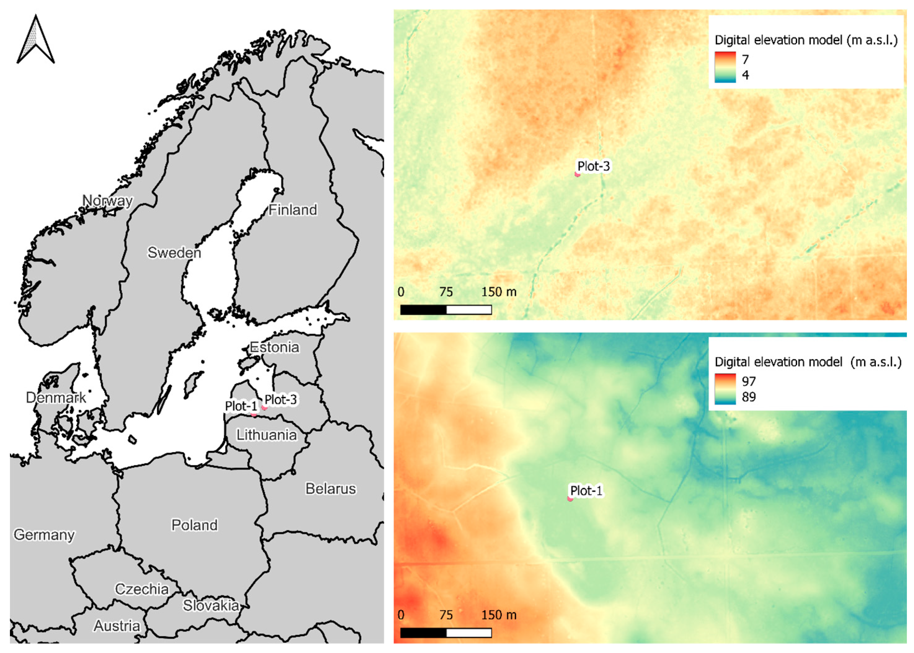
2.2. Study Site Description

According to the global ecosystem classification [26], the study sites can be attributed to different ecosystem functional groups under the temperate–boreal forest and woodland biome (T2) [27] Level 3 classification. Plot-1 is attributed to subtropical–temperate forested wetlands (TF1.2), where the black alder acts as an ecosystem engineer, building up hummocks that are not inundated, while the depressions in between are flooded for a large part of the year. Meanwhile, Plot-3 can be attributed to boreal and temperate montane forests and woodlands (T2.1), dominated by evergreen trees such as Scots pine Pinus sylvestris on a nutrient-poor rather coarse-grained soil with an intergrowth of black alder. Using other terminology, these sites can be considered as swamp–forest wetlands that experience soil oxygen depletion due to waterlogging during a significant portion of the growing season [28]. According to the EU Habitats Directive, these sites are similar to Fennoscandian deciduous swamp woods (Annex I habitat type code 9080).

2.2.1. Plot-1

Plot-1 was an elongated depression, with surrounding dryland areas about 1 to 3 m above its floor (Figure 1). The subsoil was composed of glacial sediments, mostly clay-rich till, sometimes with a thin weaner of outwash sands or glaciologic clays [29]. At nearby geological wells at a depth of 6 to 17 m from the soil’s surface, Permian limestones, Devonian sandstone and dolomite have been recovered [29,30]. Regionally, the study area is a recharge zone of artesian sub-quaternary aquifers [31], so no discharge of artesian groundwater was to be expected at the site. Site-1 had clear signs of continuous flooding, with water retreating from the soil surface only during dry summers.

The dominant tree species was the black alder. The surrounding elevated areas were dominated by a range of broadleaf species and Norway spruce (Picea abies).

The study site displayed a complicated microtopography of up to 0.5 m high peat hummocks mostly around tree stumps, with depressions in between them. The expressed microtopography provided a range of microenvironments [32], particularly providing pockets of aerated soil where uninterrupted root water uptake can take place during the events of partial flooding. A hydromorphic gley soil was found in Plot-1, with 15 cm (more in the hummocks) of black peat (O horizon, organic mater 73%) overlaying 25 cm of topsoil (A horizon), with an organic matter content of more than 9%. The soil parent material was loam to silty clay loam (according to particle size scales as defined by the USDA) glacial till diamicton parent material. Parent material below the A horizon had a light grey to bluish color that gradually changed to brownish at a depth of 2 m, indicating the reduction of trivalent (ferric) iron compounds close to the soil surface. This indicated mostly reducing but oscillating redox conditions [33]. A few fine roots were present within the soil matrix, at least up to a depth of 1.70 m.

2.2.2. Plot-3

Plot-3 was an elongated depression that lay less than 1 m below the surrounding flatland terrain. In nearby geological wells, below an about 10 m thick layer of sandy and silty sand sediments, a layer of glacial loam was recovered, overlaying upper Devonian dolomites at a depth of about 20 m [29,30]. This site was located at a reginal artesian groundwater discharge zone [34]. However, the modeled groundwater recharge was positive, i.e., water flowed into the soil [31]. Supposedly, the uppermost sand layer collects both the surface infiltration and artesian discharge and directs them towards nearby rivers.

The dominant tree species was black alder, with an admixture of birch Betula and Norway spruce Picea abies. Hydrophilic species were noted in the understory, such as common reed Phragmites australis and unidentified species from the rush family Juncaceae. The surrounding slightly elevated landscape was dominated by managed Scots pine forests.

An up to 25 cm thick organic-rich A horizon (organic matter at least 18%) was observed. The subsoil was silty sand and sand with diffuse and root-channel-associated staining of iron mineral precipitates closer to the surface and bluish tanning below a depth of about 1 m. These features suggested oscillating redox conditions and temporal anoxia [33]. A tap root with a 5 mm diameter was found even at a depth of 1.30 m, possibly extending deeper than this.

2.3. Soil Water Regime Observations

At both sites, two groundwater level loggers (at 1.0 and 2.4 m depth, Diver^® CTD or MicroDiver) were installed. In addition, volumetric soil water content probes (Meter group Teros 11 at 0.1, 0.3 and 0.6 m depths for Site-1 and 0.1 and 0.6 m depths for Site-3) and soil water potential probes (Meter group Teros 21; 0.1 and 0.6 m depths for Site-1 and at a 0.6m depth at Site-3) were installed. The measurement interval was 1 h for the groundwater pressure probes and 15 min for the soil water probes. Observations from November 2020 up to March 2023 were available. Unfortunately, the data logger for soil water probe malfunctions and observations was only available starting from October 2021.

2.4. Model Setup

One-dimensional Hydrus-1D [19] soil water models were set up for each study site. A 5 m deep 3-layer soil profile was simulated with 1001 grid nodes. The simulation periods extended from 1 January 1980 to 30 June 2022, limited by the availability of the full set (temperature, precipitation, wind speed, air humidity, radiation) of parameters in the E-OBS dataset. However, the results were analyzed for the period from 1989 to 2021, where the most complete tree-ring chronology was available, thus allowing for a 9-year model spin-up time. Potential evapotranspiration was calculated using the Penman–Monteith equation [35,36], as implemented in the Hydrus-1S software [19].

2.4.1. Modeling Scenarios: Model Instances

In this study, we sought to investigate the interaction of the soil water regime and tree growth at hydric sites (forests with waterlogged soils for a significant portion of the year). The soil water regime is governed by the temporal balance between inputs (precipitation, groundwater exfiltration and surface run-on) and outputs (transpiration, evaporation, surface run-off and export to deep groundwater). It is well established that, in the study region, additional water supply is needed apart from precipitation to maintain hydric soil conditions in a forest ecosystem [3,37]. This additional water input can be surface run-on or groundwater exfiltration. The high leaf area index (LAI) of forests enables a high transpiration rate able to evaporate more water than the precipitation input in the study region [3]. Therefore, we designed model scenarios with a range of water inputs and a range of active proportions of LAI (kLAI). It has been shown that LAI is one of the most important parameters determining the forest water balance [16], where a high LAI corresponds to a high transpiration water demand.

We considered a simple conceptual model, where the constant-rate groundwater exfiltration was a single additional water source in the model domain, providing positive bias for the soil–water balance. After considering a range of preliminary model configurations with seasonal groundwater seep-in or run-on patterns [38], a simpler constant groundwater exfiltration boundary condition was selected. This simpler model configuration provided comparable results to more complicated seasonal additional water input conceptualizations. Four groundwater exfiltration scenarios were defined with 0, 0.01, 0.03 and 0.05 cm day⁻¹ flow rates (SeepIn).

Potential transpiration rate is controlled by active leaf area, which is expressed as LAI. It is difficult to quantify LAI accurately. In temperate forests, it is highly variable and effects such as self-shading can render only some of the leaves as participating in transpiration. [39]. In this study, we obtained the LAI from a remote sensing data product [40] (see Section 2.8 with a nominal 300 m pixel size, exceeding the dimensions of the study plot. In addition, the actual active LAI value would be sensitive to ecosystem feedback and internal dynamics. Therefore, we investigated a range of scenarios where the daily LAI value was multiplied by a coefficient, kLAI (0.4, 0.5 and 0.7), to obtain the active LAI value.

For each study site, we defined 12 unique combinations of SeepIn and kLAI as model scenarios and invoked a corresponding number of unique model instances. The SeepIn and kLAI values were selected so that the range of respective model outputs, particularly the depth to the groundwater, enveloped the actual observations. Thus, we investigated the parameter space for the two crucial factors apart from actual meteorological conditions controlling the terrestrial ecosystems’ water balance.

2.4.2. Model Calibration and Uncertainty

We performed manual model calibration using the trial and error method. First, the soil water retention curve parameters measured in the laboratory were modified to resemble observed soil water potential and content ranges. Then, the ranges of the two most important, but uncertain, parameters governing the water balance—groundwater exfiltration and active leaf area—were explored. As a result, we selected a set of these parameters where the model output envelopes actually observed soil water regime for further analysis. Other studies using the Hydrus-1D model have employed similar manual calibration approaches [41].

The model uncertainty arose from model parameter uncertainties as well as from input data uncertainties. To gain a estimate of the calibrated model uncertainty, we assumed that the true output value could be anywhere (uniform distribution) between two model instances enveloping the model instance closest to observations. We calculated the difference between these model instances, converted it to standard distribution dividing by $\sqrt{3}$ and multiplying by 1.96 to obtain uncertainty at 95% confidence level (1):

$$U_p=\frac{1.96}{\sqrt{3}}\frac{{\sum }^{ }\left(p_{m1}-p_{m2}\right)}{N}$$

(1)

where $U_p$ is uncertainty for parameter $p$, $N$ is the number of years values and $p_{m1}-p_{m2}$ is the difference between mean parameter value two enveloping model instances from May to August (the season considered in the later analysis).

2.4.3. Soil Hydrological Properties

The soil hydrological properties—the water retention curve and hydraulic conductivity—were measured in the soil samples from shallow wells and excavations, targeting the depth intervals from 0 to 10cm, 20 to 30 cm and 40 to 60 cm. Soil monoliths were collected in 5 cm high 100 and 250 mL stainless steel cylinders along with unstructured samples.

The saturated hydraulic conductivity was measured according to the falling head method with an Eijkelkam Soil water permeameter [42] in 100 mL cylinders. The grain-size distribution, organic matter content and density of the solid particles of the unstructured samples were measured in line with the ISO 17892-4:2017, EN 13039:2012 and ISO 17892-3 standards, respectively, in a commercial laboratory.

The water retention curve and unsaturated hydraulic conductivity were determined using a Meter Hyprop2 system, which used two micro tensiometers to measure the water potential gradient in a sample that was subjected to air-drying [43]. The application of the boiling delay technique using degassed deionized water in the tensiometers extended the theoretical measurement range of the soil water potential up to −200 kPa. The estimated air-entry pressure (about −8800 kPa) of the tensiometers’ ceramic cup was set as an additional data point [44]. The micro tensiometers were filled with deionized and manually (with a syringe) degassed water. The samples were saturated by immersing them in deionized and degassed water. The initial sample water content during the analysis was estimated from the dry weight of the sample after the analysis by drying for 8 to 24 h at 105 °C.

The soil water retention and unsaturated hydraulic conductivity were described via the van Genuchten functions [45] using the Meters HYPROP-FIT software [46]. A unimodal pore size distribution was assumed. Clay-rich samples of the subsoil from Plot-1 expanded upon saturation by about 5%, which was already comparable to the plant-available water for the range between 0 and −1500 kPa for the soil water potential. To compensate for this deviation, in natural conditions, field measurements of the soil water content and potential were used to constrain the fitting of the van Genuchten parameters in HYPROP-FIT software. The resultant soil properties are presented in

Table 2. Soil properties.

			Soil Composition (% Dry Weight)				Van Genuchten–Mualem Parameters
Site	Depth (cm)	Model Layer No.	Org. Mater	Sand	Silt	Clay	Qr (cm3 cm−3)	Qs (cm3 cm−3)	Alpha (cm−1)	n	Ks (cm day−1)	l
Plot-1	0.02–0.07	1	73%				0.244	0.899	0.224	1.405	1898.8	−0.797
Plot-1	0.25–0.30	2	8.6%	15.6	60.2	24.2	0.250	0.507	0.3377	1.149	424.7	−1.474
Plot-1	0.63–0.68	3	3.1%	27.9	46.6	25.5	0.290	0.41	0.0200	2.000	1.08	−0.797
Plot-3	0.02–0.07	1	18.5%	68.8	31.2	0.0	0.026	0.817	0.0251	1.380	731.1	5.317
Plot-3	0.12–0.17	2	18.5%	68.8	31.2	0.0	0.075	0.656	0.0328	1.305	172.1	1.718
Plot-3	0.61–0.65	3	0.9%	94.5	5.5	0.0	0.029	0.375	0.0200	1.835	6.08	0.391

.

2.5. Meteorological Data: E-OBS

The model was forced using data from a gridded meteorological observation dataset E-OBS [47], version 26.0e. However, the v26.e version had unrealistically low precipitation for the study locations from 2009 to 2012 in comparison to the observations in nearby meteorological stations and the E-OBS v25.0e version. Therefore, we imputed the time series for these years from E-OBS v.25.0e into the dataset of E-OBS v26.0e. Data regarding daily mean wind speed, relative humidity, global radiation, precipitation and mean minimal and maximal air temperature for the respective grid cell were extracted. The E-OBS dataset was selected as a source for meteorological conditions as there were no meteorological station data available in the vicinity of the study site; the closest meteorological station in Dobele with long-term observations was about 30km from the site.

2.6. Root Depth Distribution

Rooting depth is a critical constraint of the soil water volume accessible to plants in periods when potential evapotranspiration exceeds precipitation; generally, it is a function of plants’ water acquisition strategies and local hydro-geomorphological conditions [48]. The authors of [49] proposed an empirical power Equation (2) to describe the cumulative proportion of fine root biomass ($y$) as a function of depth in cm ($D$) with a species-specific constant $\beta$. The authors of [50] estimated the value of the $\beta$ parameter for major biomes including boreal, temperate coniferous and deciduous forests (0.943, 0.980 and 0.967, respectively). We used the transformation (3) of (2) to describe the instantaneous root fraction for temperate deciduous forests (

Table 3. Relative fine root proportion at different depths for temperate deciduous forests from [50].

Depth (cm)	Boreal	Temperate Deciduous	Temperate Coniferous
0	1.00	1.00	1.00
25	0.23	0.43	0.60
50	0.053	0.19	0.36
100	0.0028	0.035	0.13
200	0	0.0012	0.018

). Similar exponential root depth distributions have been used in other root water uptake studies, for example [51]. The root depth was cut off at 1 m below the surface.

$$y=1-{\beta }^D$$

(2)

$$\frac{dy}{dD}=-{\beta }^D\ln \beta$$

(3)

2.7. Root Water Uptake Parameterization

Root water uptake is part of a complex interaction between soil, plants and the atmosphere, where the water in soil pores moves towards plant roots, is absorbed by plant roots (often assisted by rhizosphere fungus), transported in the plant in the xylem, evaporated in the air space between cells in the leaves and released into the atmosphere via stomata by means of diffusion. Any of the elements in this chain can limit the overall transpiration rate and, by extension, root water uptake [52].

In this study, a simplified parametrization of root water uptake proposed by [53] was used as implemented in the Hydrus-1D model [19]. In short, the root water uptake is expressed as a trapezoid function of the soil water potential. If the soil water potential is above a certain arbitrary “anaerobiosis point” (h₀), no root water uptake takes place. However, if the water potential is less than this point, the water uptake rises sharply to reach its full potential quickly (h₁) and remains as high as the second infliction point (h₂) if the potential evapotranspiration is above some arbitrary threshold or (h₃) if it is below it. As the soil water potential further decreases, root water uptake is reduced to zero at the wilting point (h₄). In addition, following [54,55], a root adaptability factor is introduced, allowing for the compensation of reduced root water uptake in stressed parts of the root zone by increased uptake in non-stressed parts [19].

Alternatively, it has been suggested that simpler, and perhaps more realistic [56], root water uptake for variable soil water potential can be described by an S-shaped curve proposed by [57], requiring fewer parameters. However, this representation does not include a reduction in the root water uptake from waterlogged (anaerobically stressed) soils and thus was not suitable without modification for the given study of hydric forests.

In a theoretical study comparing a physically based root water uptake model [58] and several empirical models, Ref. [51] found that the optimal fitted parameters for the empirical models depended on the root density by soil volume, potential transpiration rate and soil type, in addition to plant characteristics. Thus, it appears that the optimal numerical values of empirical parameters, to some extent, are determined by their interaction with a range of processes. From this consideration, it follows that site-specific parameters determined elsewhere derived from the literature are of little use for a particular case study. This ambiguity can be identified in the scientific literature; for example, Ref. [59], in their model of apple tree root water uptake, obtained the Feddes’ parameters (h₀, h₁, h₂ and h₃ representing 0, −0.1, −10.0 and −150.0 m, respectively) from [60], who further referred to the original work of [53].

The roots of the black alder can grow below the water table in oxygen-deprived soil or directly in the water [61]. The tree tends to maintain high transpiration levels even if the topsoil is desiccated, drawing the water from deeper within the soil or groundwater [62]. In this study, we set the Feddes’ model parameters so that root water uptake was initiated at 0 soil water potential but decreased at a relatively high water potential (h₀, h₁, h₂, h₃ and h₄ representing 0, −2, −200, −200 and −5000 cm, respectively). We set the critical stress index to 0.5, so that water uptake was largely compensated by non-stressed parts of the root system [54].

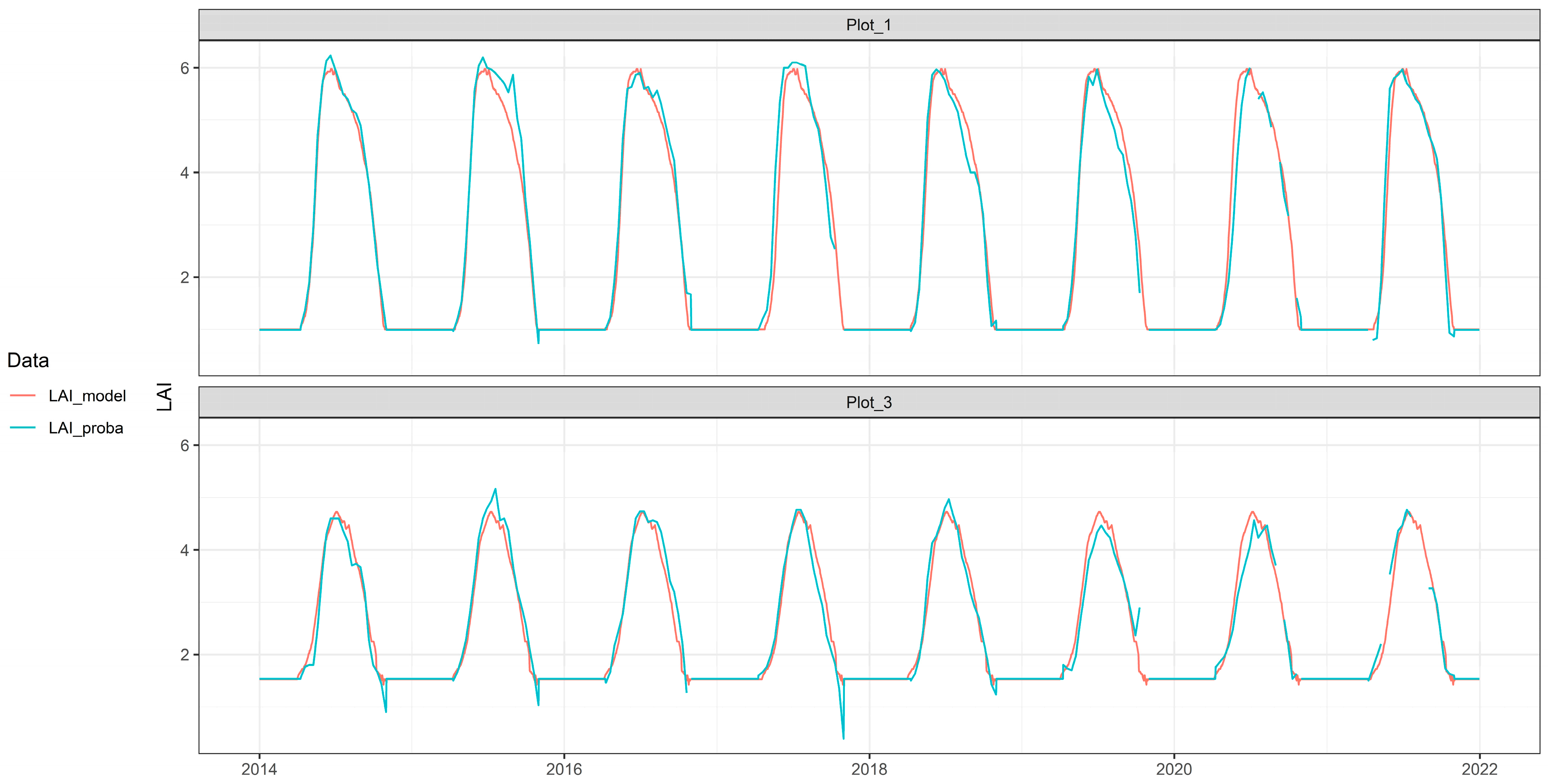
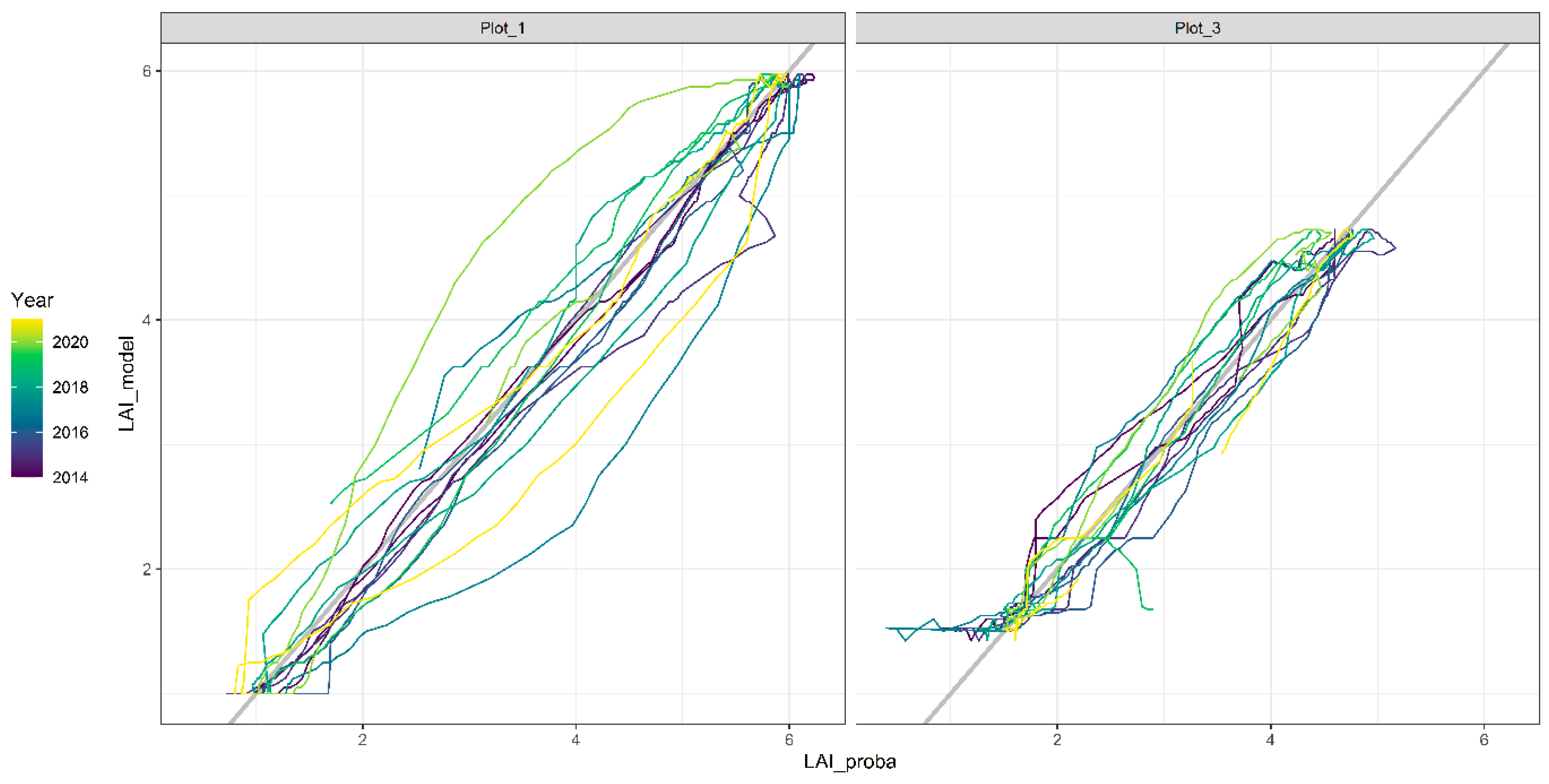
2.8. Leaf Area Index (LAI) Seasonal Trajectory Model

Leaf area index (LAI) is a crucial parameter for the forest water balance, as it influences both transpiration and interception. In a review examining global pine forest water balance, [16] found that LAI was the most important parameter (more important than photosynthetically active radiation (PAR)) in explaining the variations in canopy transpiration.

In this study, LAI was obtained from the Copernicus Global Land Service, hosted by the VITO NV based in Belgium (https://land.copernicus.vgt.vito.be; last visited on 2 September 2022 [63]), derived from PROBA-V (version 1.0), a miniature ESA satellite, and a Sentinel-3 Ocean and Land Colour instrument (OLCI; version 1.1) covering the period from 2014 to 2021. As a remote sensing product, this included all the green plant surfaces including understory vegetation [40] and LAI was expressed as half of the total green photosynthesizing surface, i.e., half of the total area of both sides of a flat leaf. LAI was provided on decadal (10-day) time steps; each time step represented the composite LAI value for the 10-day period before and after the given date in 0.003-degree (~300 m) resolution [40]. During the winter period, there were gaps in the 10-day LAI value time series.

It is well established that spring phenology in temperate humid climates is mostly temperature driven. So-called thermal time or degree day models are often used to predict the leaf-out dates [64,65]. This is consistent with the negative (early) trend for leaf-out dates in the study region [66]. There are some suggestions that the atmospheric water vapor pressure is a similarly important driver of spring phenology, but it is largely correlated with air temperature [67].

However, autumn phenology—leaf senescence—is more complicated and no clear patterns have emerged in the study region regarding leaf senescence [66]. This is in line with common assumptions that the day length and air temperature [68] are the main drivers, although the role of internal development (e.g., competence to senescence) has also been recognized [69]. Recently, it has been suggested that autumn senescence might be regulated by the sink limitation of photosynthesis [70]; as a result, early leaf-out and favorable growing conditions during the summer can result in earlier leaf senescence, irrespective of the air temperature in autumn, a phenomenon that has been widely studied for herbaceous plants (e.g., [71]).

2.8.1. LAI Model

The LAI seasonal trajectory was calculated using a simple degree day model for spring phenology that was used to stretch the long-term average seasonal trajectory, adjusting the start of the growing season:

• As there were large gaps in the available LAI observations during winter, the winter background LAI value ($LA{I}_w$) was calculated as the average of a few available LAI observations between days of the year from 320 to 100. This value was interpreted as green parts of conifers and overwintering bryophytes.
• Continuous daily LAI time series were obtained by linearly interpolating the available LAI observations.
• The start of the vegetation season ($S_{start}$) was assumed to be the day of the year when the LAI value in spring exceeded that of the winter LAI by 1.5 ($LA{I}_w+1.5$).
• Furthermore, all the available observed seasonal LAI trajectories were aligned to match the start of the vegetation season ($S_{start}$); the master seasonal trajectory ($LA{I}_{master}$) was calculated as the daily median of the aligned LAI value for each day of the year except for winter (days of the year from 320 to 100).
• The start of the vegetation season ($S_{start}$) for each year was calculated using a simple degree day phenological model [64,72]. 1 January was set as the start of the degree day accumulation ($t_1$) and the phase onset was assumed to match the date when the active temperature sum ($DD$) exceeded the predefined value for daily average temperature ($T_{avg}$) and base temperature ($T_{base}$) (4):

  $$DD={\displaystyle \sum }_{t=t_1}^{t=t_2}{T}_{avg}-T_{base}$$

  (4)
• The aligned master trajectory ($LA{I}_{master}$) was compressed or stretched to match the fixed end date (31 December) via proportionally thinning (removing an appropriate number of evenly spread daily LAI data points) or upscaling (inserting an appropriate number of new daily data points interpolating the LAI value), respectively, for late or early springs.
• The most appropriate base temperature ($T_{base}$) and critical degree day ($DD$) parameter set was selected by generating a range of base temperature ($T_{base}$) and critical degree day ($DD$) values and selecting values that produced LAI trajectories with the least RMSE (root mean squared error) when compared to the observations.
• Finally, the LAI seasonal trajectory for the model period was calculated with daily average temperature from the E-OBS dataset as the input.

2.8.2. LAI Seasonal Model Results

The best parameters for the LAI seasonal trajectory are presented in

Table 4. Best-fit parameters for the LAI seasonal trajectory model.

Site	RMSE *	${\mathit{T}}_{\mathit{b}\mathit{a}\mathit{s}\mathit{e}}$	$\mathit{D}\mathit{D}$	$\mathit{L}\mathit{A}{\mathit{I}}_{\mathit{w}}$	${\mathit{S}}_{\mathit{s}\mathit{t}\mathit{a}\mathit{r}\mathit{t}}$ (DoY)
Plot-1	0.36	2.5	260	0.99	129
Plot-3	0.21	1	565	1.53	147

* RMSE—root mean squared error

. The yearly LAI seasonal trajectories are presented in Figure 2. Finally, a visual comparison of the observed and modeled trajectories is provided in Figure 3.

2.9. Albedo

Albedo is an important element of the energy budget indicating the amount of radiation energy that is dissipated due to reflection. The surface albedo data were obtained from the EU Copernicus program SPOT/VEGETATION and its successor, the Proba-V satellites; the hemispherical surface combined near infrared and visible albedo at 1/112° (~1 km) resolution [73,74].

For Plot-1, the canopy reflectance (albedo) was between 0.1 and 0.2, while for Plot-3, it was between 0.09 and 0.16 (Plot-3) for most of the year but jumped to above 0.4 when snow cover was present. According to the E-OBS data, the incoming solar radiation was only about 20% of the year average radiation for the three winter months (December, January, February). Variation of the surface albedo by about 0.3 units would impact the overall radiation budget by less than 6%. Therefore, it was concluded that the snow’s impact on the albedo, and thus the energy budget, could be neglected. Similarly, if we were to adopt a dynamic albedo value based on leaf phenology for the period from March to November, ranging between 0.1 and 0.2, instead of a fixed average value between these two values, the overall impact on the energy budget would be less than 10%. Therefore, a monthly radiation-weighted average albedo for each study site was calculated: 0.17 for Plot-1 and 0.12 for Plot-3.

2.10. Interception

Interception is the process of the vegetation trapping rain droplets before they reach the soil surface. Experimentally, it is usually measured as the difference between clear sky rainfall and rainfall below the canopy [16]. However, the heterogeneity of the canopy resulting in different throughfall at different locations and stemflow [75] can complicate this approach. Even more so, when a rain droplet hits a leaf surface, it disintegrates and some smaller daughter droplets can be transferred back into the atmosphere. In addition, as soon as the rainwater has been intercepted by the leaf, it can start to evaporate, using the sensible heat energy stored in the biomass or air [75].

In the Hydrus model, the canopy interception is calculated as a function of LAI, supplemented by an empirical parameter, the interception parameter [19]. In this study, we used the recommended empirical value of 0.25 mm/d as implemented in the SWAP model [76]. This value was empirically determined in the Netherlands for common crops. However, in other forest studies considering beech (Fagus sylvatica L.) and Norway spruce (Picea abies (L.)), considerably higher interception values (1.5 to 2 mm/day) have been used [77,78].

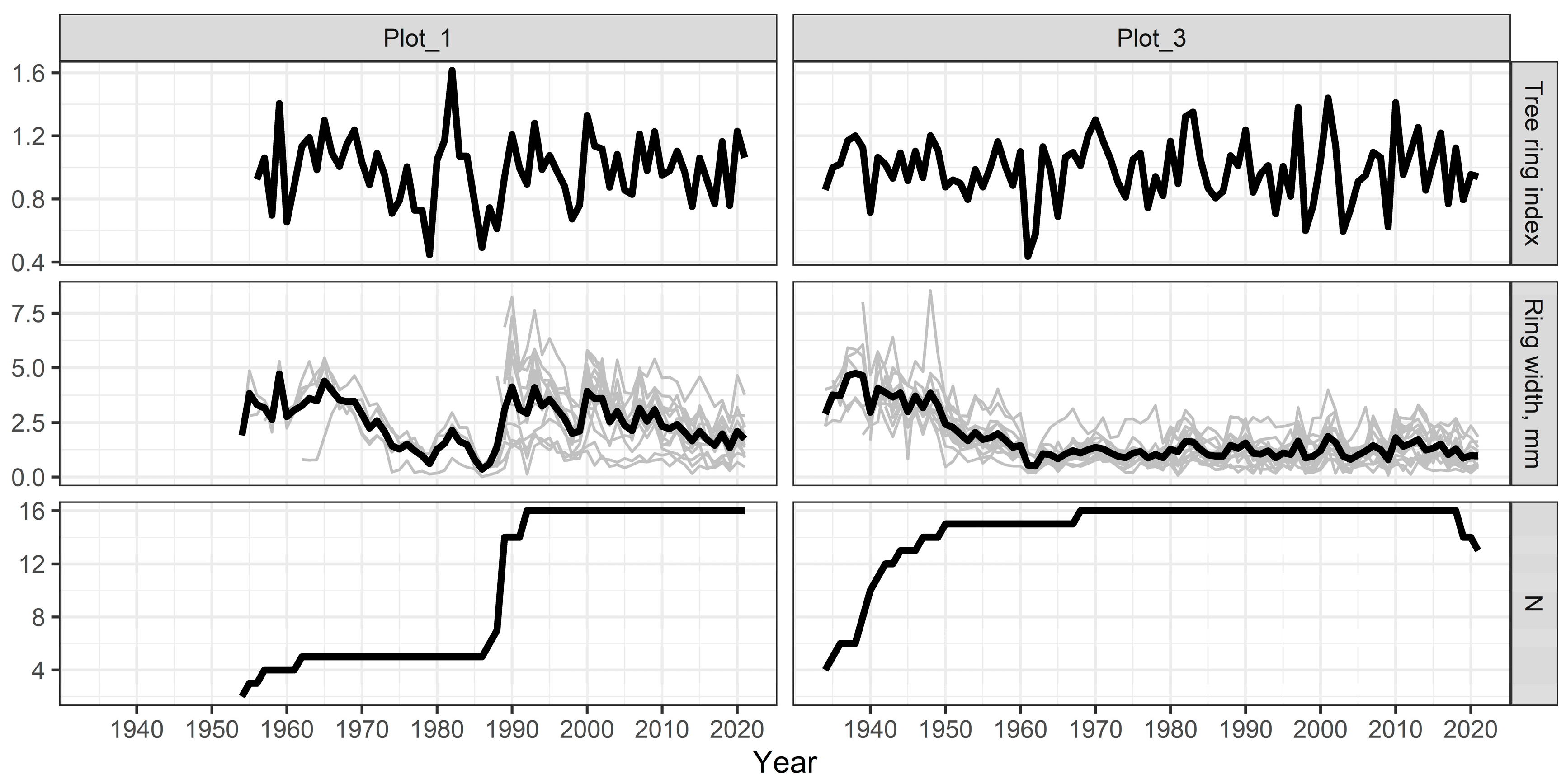
2.11. Tree-Ring Chronology

The field campaign was carried out in spring 2022. Black alder trees were selected in two sampling sites. A total of 30 individuals of black alder were sampled (15 individuals at each sampling plot), in line with the guidelines provided by [79]. Trees were cored with a standard 5 mm increment borer, taking one or, in most cases, two opposite cores at DBH. The cores were air-dried and gradually sandpapered (from 80 to 500 grade) to produce a flat and polished surface where tree-ring boundaries were easily identified under magnification. Tree-ring widths were measured with an accuracy of 0.01 mm using a linear table Lintab and the TSAP-Win program [80]. The accuracy of the visual cross-dating and the existence of measurements errors were examined using the program COFECHA [81], which calculates cross-correlations amongst individual series of tree growth.

To assess the influence of hydrology on the growth of black alder, for each sampling plot, tree-ring width series were detrended using a modified negative exponential curve, using the package dplR [82] in program R [83]. These were then combined to build a residual chronology after applying auto-regressive modeling [84]. Thus, a detrended time series was obtained, emphasizing year-to-year variability and omitting tree age and other long-term controls of the ring width.

2.12. Analysis and Interpretation

The interaction of the tree-ring-width increment with meteorological and modeled hydrological parameters was assessed using Pearson’s product moment correlation. The uncertainty of the correlation was calculated for a 95% confidence level in R (function cor.test, [85]). To assess the importance of the soil water regime variations throughout the growing season, we considered mean parameter values for a sliding-window period from May to August (May, May–June, May–July, May–August, June–August, July–August, August).

The considered monthly mean meteorological parameters were wind speed (Wind, km/day), precipitation (Prec, cm day⁻¹), solar radiation (Rad, MJ m⁻² day⁻¹) and daily mean temperature (Temp, °C). High wind speeds due to increased boundary layer mixing can increase evapotranspiration. Precipitation provides crucial ecosystem moisture input, but, if excessive, can cause soil waterlogging detrimental to tree growth. Solar radiation is the primary energy source both for photosynthesis and evapotranspiration. Air temperature is another primary factor controlling both vegetation development and evapotranspiration. These data were extracted from the E-OBS dataset [47].

The considered monthly mean modeled soil water parameters were the depth to groundwater from soil surface (GWdepth, cm), difference between maximum and minimum depth to groundwater (rangeGWdepht, cm), potential root water uptake (rRoot, cm day⁻¹), actual modeled root water uptake (vRoot, cm day⁻¹) and ratio between actual and potential root water uptake (vRoot_rRoot). A groundwater table close to the soil surface indicates waterlogged soil conditions, while a moderately deep groundwater can provide an additional water source for the vegetation. It has been reported that high fluctuations in the depth to groundwater can negatively affect the radial growth due to stressed root systems [86]. The potential root water uptake is the amount of water that would be needed to fully support transpiration demand under given meteorological conditions, while the actual root water uptake is the measure of the water that the vegetation is able to extract from the soil given the soil water potential and model constraints for the root water uptake. vRoot can be considered a proxy for primary production, as the exchange of water vapor and CO₂ across stomata is proportional for given meteorological conditions. For each of the study plots, the results from 12 model instances with different values for kLAI (proportion of active leaf area index) and groundwater exfiltration were examined.

3. Results

3.1. Tree-Ring Chronology

Here, we briefly present the tree-ring chronologies (Figure 4) for the two study plots and then explore correlations between yearly tree-ring increment and meteorological and soil water parameters.

3.1.1. Plot-1

In Plot-1, the black alder tree-ring chronology started in the early 1950s. However, it was initially represented by only five trees, while most of the other trees appeared to be established shortly before 1989. The tree-ring-width increments gradually decreased, indicating the maturation of new tree stems. The presence of decayed tree stumps indicated a logging event during this time; trees regrew from new roots and stem shoots. Some of the older tree population survived this forest clearing event.

3.1.2. Plot-3

In Plot-3, the current black alder population appeared to have been established in the 1930s or shortly before that. Initially, the yearly tree-ring growth increments were wide but gradually declined up to 1960; since then, the yearly ring width has remained relatively stable.

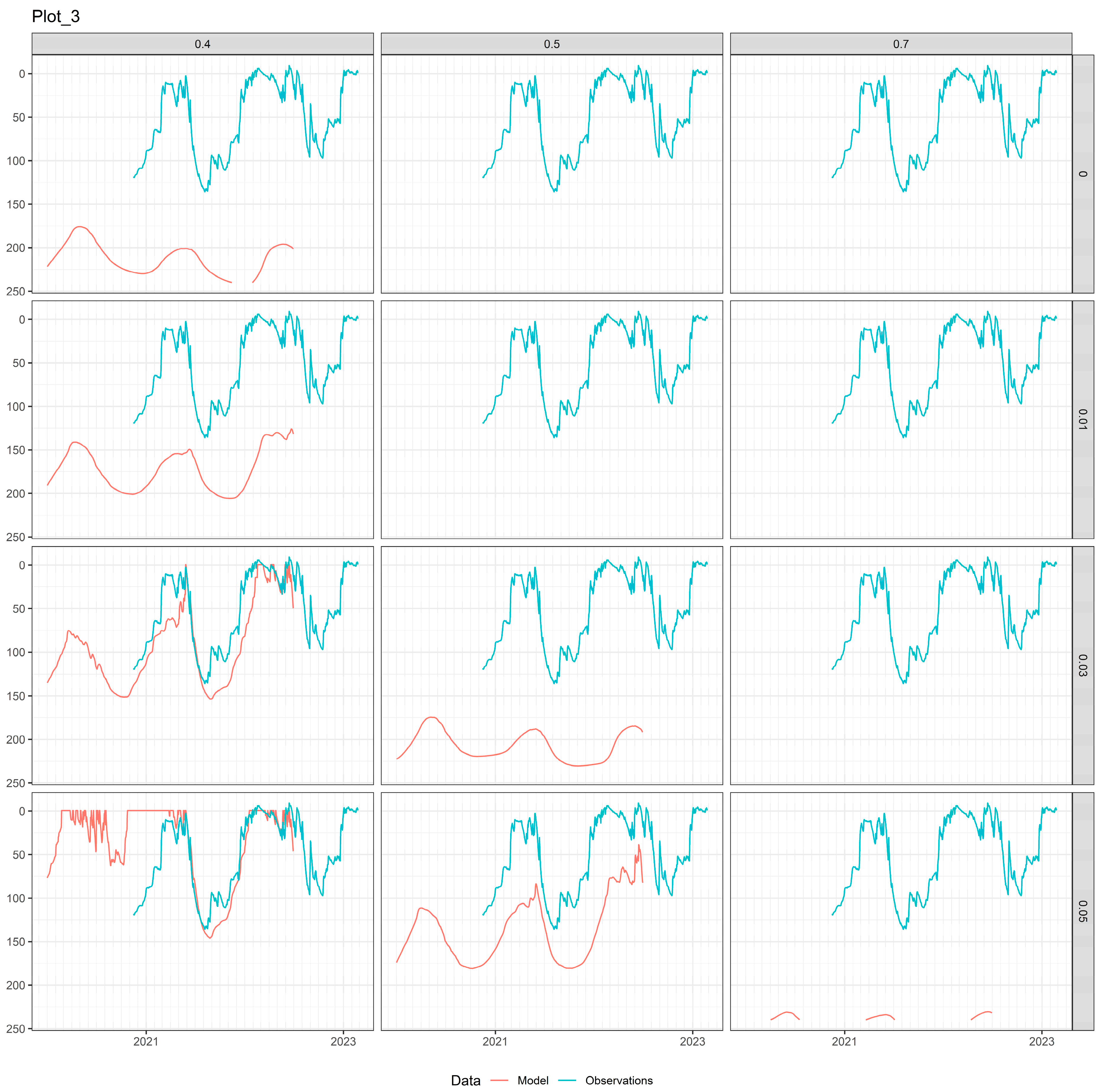
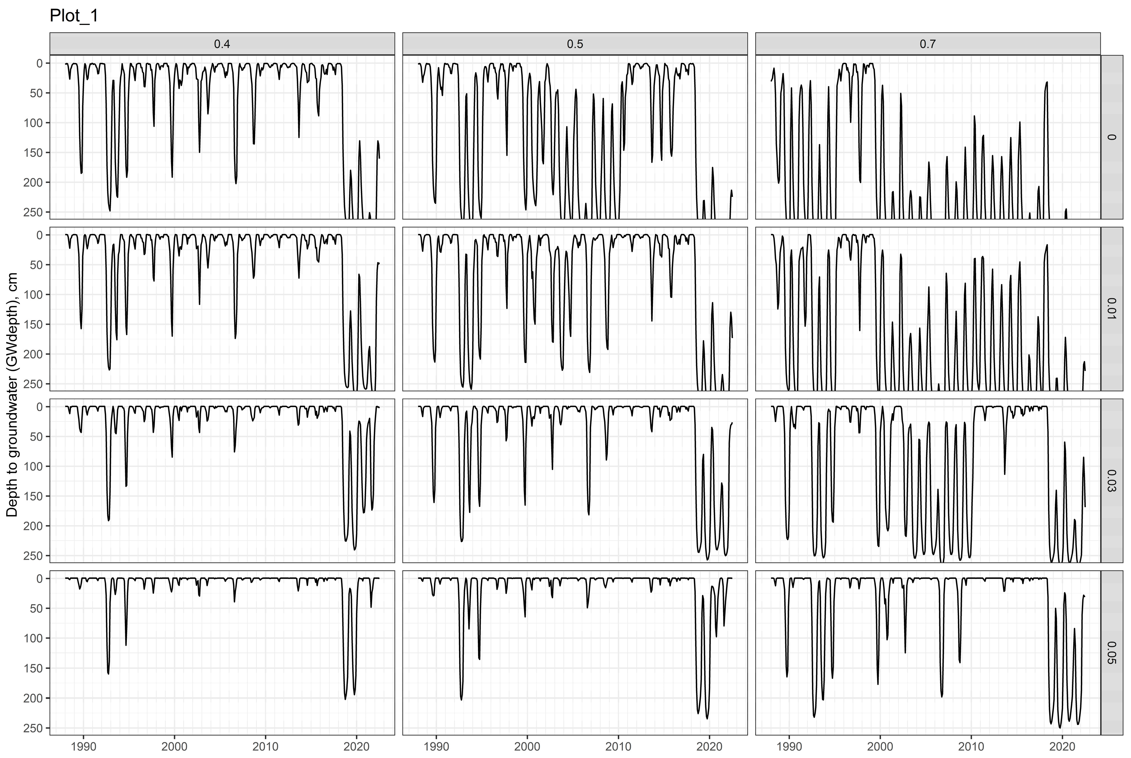
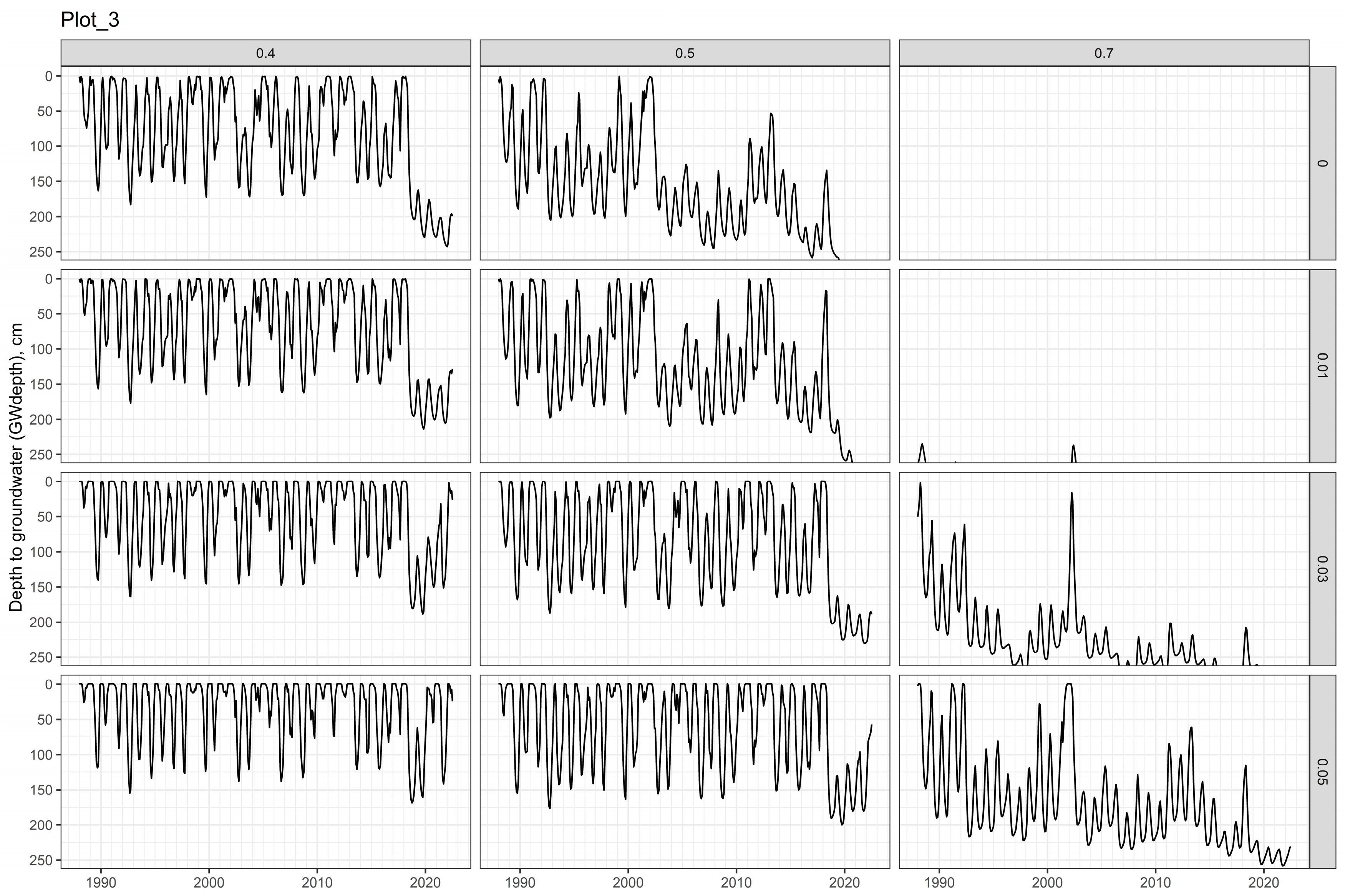
3.2. Soil Water Models

For each of the study sites, 12 instances of the Hydrus-1D soil water model were invoked. Each model instance had a unique combination of the active LAI proportion (kLAI equal to 0.4, 0.5 or 0.7) and groundwater exfiltration (SeepIn equal to 0, 0.01, 0.03 and 0.05 cm day⁻¹). Each model configuration was selected after a range of test model runs (not shown) to examine a range of possible soil water regimes in these hydric sites. The model results were then compared to the actual soil water observations and tree-ring chronology for each study site.

According to the root mean squared error (RMSE) for groundwater head at a 240 cm depth for Plot-1, the best-performing model had a kLAI of 0.5 and groundwater exfiltration of 0.05 cm day⁻¹, while, for Plot-3, the best-performing model had a kLAI of 0.4 and exfiltration of 0.03 cm day⁻¹ (

Table 5. The root mean squared error (RMSE) of groundwater head (cm) at a 240 cm depth. Notice that, for each of the two case studies, a group of higher-performing models stand out with a relatively small proportion of active leaf area (kLAI) and a larger additional moisture in-flow in the form of groundwater exfiltration (SeepIn), thus indicating that reduced transpiration and/or a high water supply are needed to maintain the observed wetness levels of the study sites.

Site	SeepIn (cm day−1)	Par	kLAI
			0.4	0.5	0.7
Plot-1	0	h_240 cm	250	280	320
Plot-1	0.01	h_240 cm	200	240	270
Plot-1	0.03	h_240 cm	74	170	210
Plot-1	0.05	h_240 cm	29	18	160
Plot-3	0	h_240 cm	170	280	NA
Plot-3	0.01	h_240 cm	120	230	300
Plot-3	0.03	h_240 cm	31	160	230
Plot-3	0.05	h_240 cm	42	79	200

). Model performance according to other observed soil water characteristics (water content and potential) and metrics (RMSE, mean signed difference and R-squared) was similar, albeit less robust (Supplementary Material, Table S1). However, the groundwater head was the most robust parameter describing the soil water regime in wetlands; therefore, we primarily used it to evaluate the model performance.

Comparing the model output to the observed groundwater level, we observed that model instances with a moderate to small kLAI generally reproduced the observed groundwater level better than model instances with a high kLAI (Figure 5 and Figure 6). In the case of Plot-1, the simulated groundwater head was closest to the observations for the model instance with the highest tested groundwater exfiltration (0.05 cm day⁻¹) and a moderate kLAI (0.5; Table 5). In the case of Plot-3, the model that performed best had moderate groundwater input (0.03 cm day⁻¹) and the lowest kLAI (0.5).

We estimated that the mean uncertainty for the period from May to August in analyzed years from 1989 to 2021 of the model with best representation of the observed conditions in terms of depth to groundwater was 14 and 25 cm for Plot-1 and Plot-3, respectively. The estimated range from depth to groundwater was 22 and 16 cm and the root water uptake was 0.02 and 0.08 cm day⁻¹.

As expected, model instances with a higher kLAI and less groundwater exfiltration produced results with limited or no waterlogged soil conditions (Figure 7 and Figure 8), while models with smaller kLAI values and a higher groundwater input displayed predominantly waterlogged soil conditions. Particularly, in Plot-3, the model instance with a kLAI of 0.7 and low groundwater exfiltration produced a dramatically low groundwater table and local groundwater recharge only during the wettest of years (Figure 8). Such model behavior indicated that all incoming precipitation was stored as soil–pore water and that capillary rise into the root zone through subsequent root water uptake consumed the groundwater exfiltration. Interestingly, several model instances of Plot-1 produced a higher range of groundwater level fluctuations, with multiyear periods of low or high average groundwater. In the same time period, the year-to-year fluctuations of the groundwater and soil water regime for Plot-3 were more stable. It must be noted that the drought years of 1992 to 1994 and 2018 and 2019 stood out prominently in the modeled water regime in both study sites. The former period has been noted as a groundwater drought in the Baltic region [87], while the latter two years are well known European drought years [88]. Overall, it can be noted that progressively dryer conditions, displaying a deeper average groundwater table, were simulated towards the end of the study period.

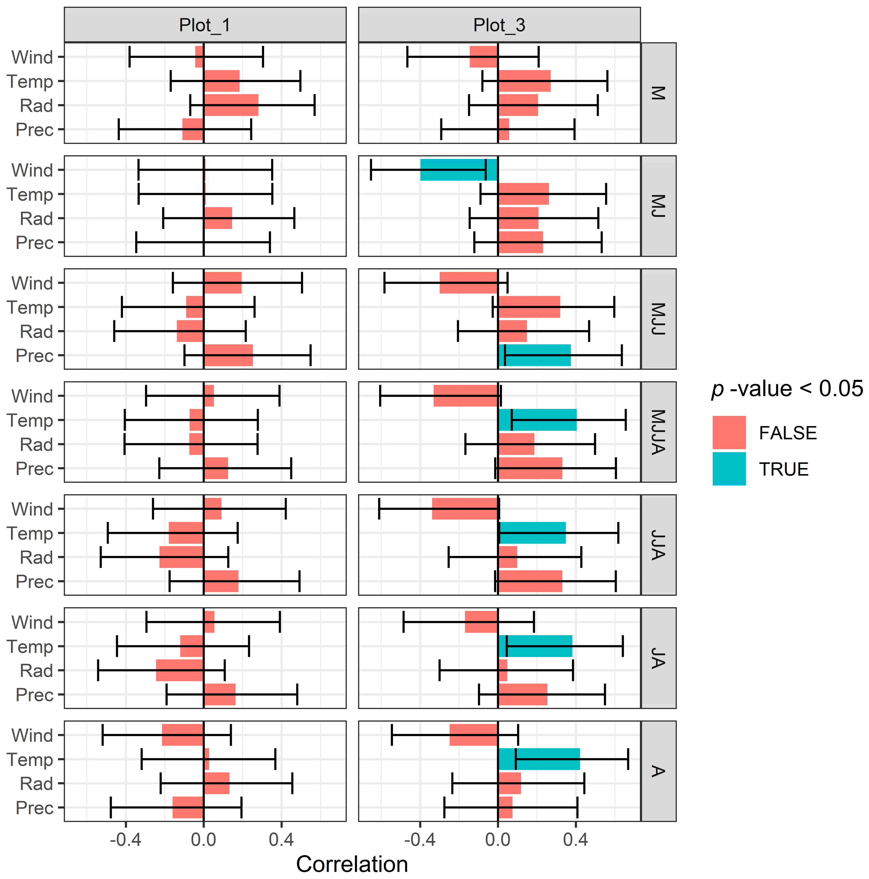
3.3. Correlation between Meteorological and Soil Water Conditions and Tree-Ring Chronology

The overall length of the black alder tree-ring chronology in Plot-1 was 68 years, starting in 1954, while in Plot-3, the chronology length was 90 years, starting in 1932 (Figure 4). The number of sampled trees in Plot-1 rose sharply in 1989. Apparently, at this point, a regrowth of black alder took place after forest clearing. Such a forest-management action would significantly affect the water regime and therefore would not be represented in our model with static stand characteristics. In addition, the forest floor’s hydrological properties can change significantly after forest clearing and can recover gradually over the course of a period of several years [89]. Therefore, for the sake of consistency, we limited the analysis for both study sites to a 32-year period from 1989 to 2021.

3.3.1. Meteorological Conditions

In the case of Plot-1, the tree-ring increment displayed no significant correlations with meteorological parameters (Figure 9, Supplementary Materials Table S2). However, a tendency could be noted in which higher temperature and radiation in May were associated with higher tree-ring increments, which reversed later in the season.

In the case of Plot-3, the tree-ring increment’s correlation with meteorological parameters was overall higher; notably, temperature had a significant positive correlation with tree-ring increment during most of the growing season, except at its start (Figure 9). Precipitation had a significant positive correlation with tree-ring increment at the beginning of the summer. Interestingly, wind speed had a negative correlation with tree-ring increment. For some parameters and time intervals, opposite signs of correlation were observed. However, these were not significant at a 95% confidence level and therefore might not represent any real relationship.

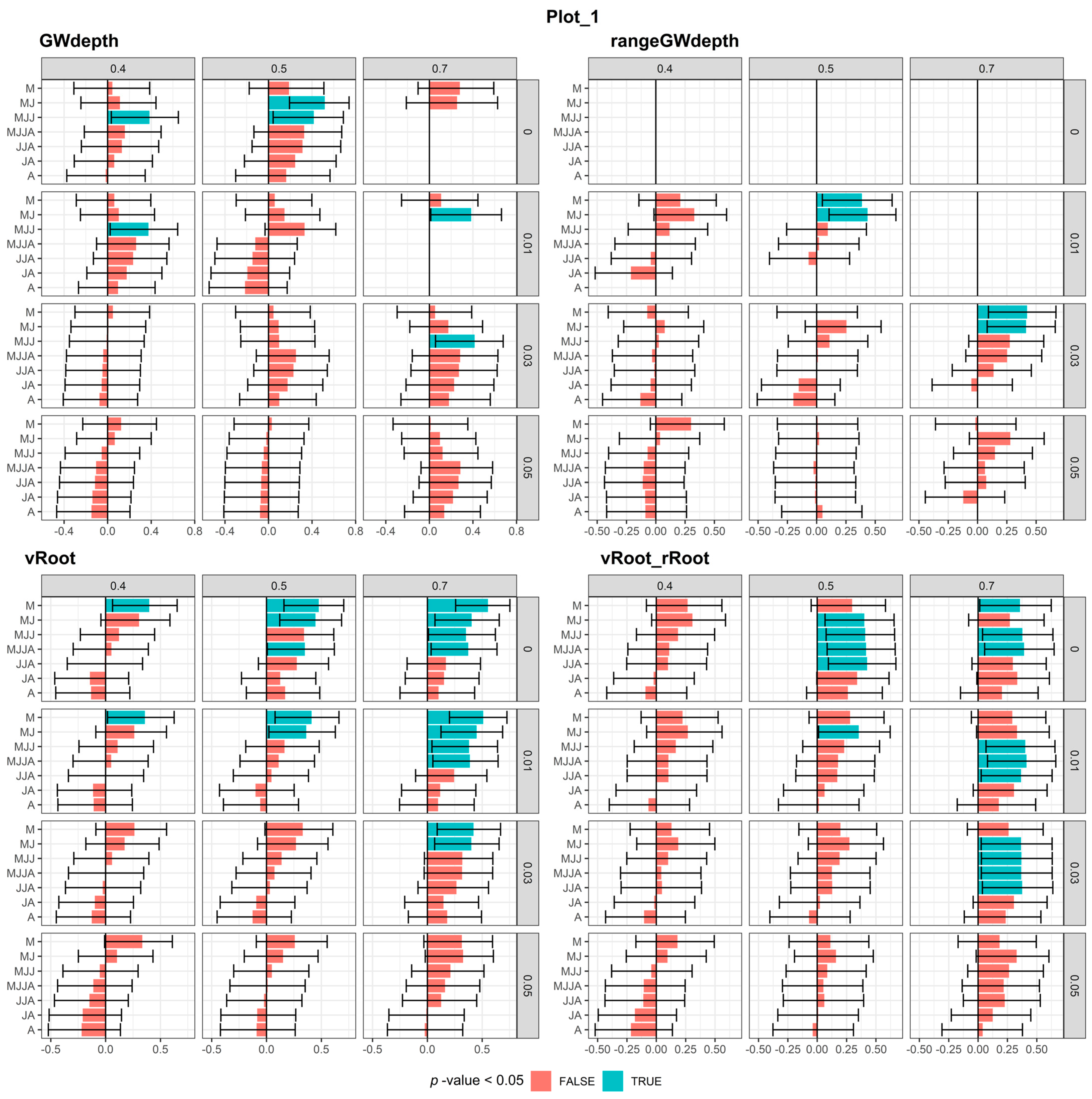
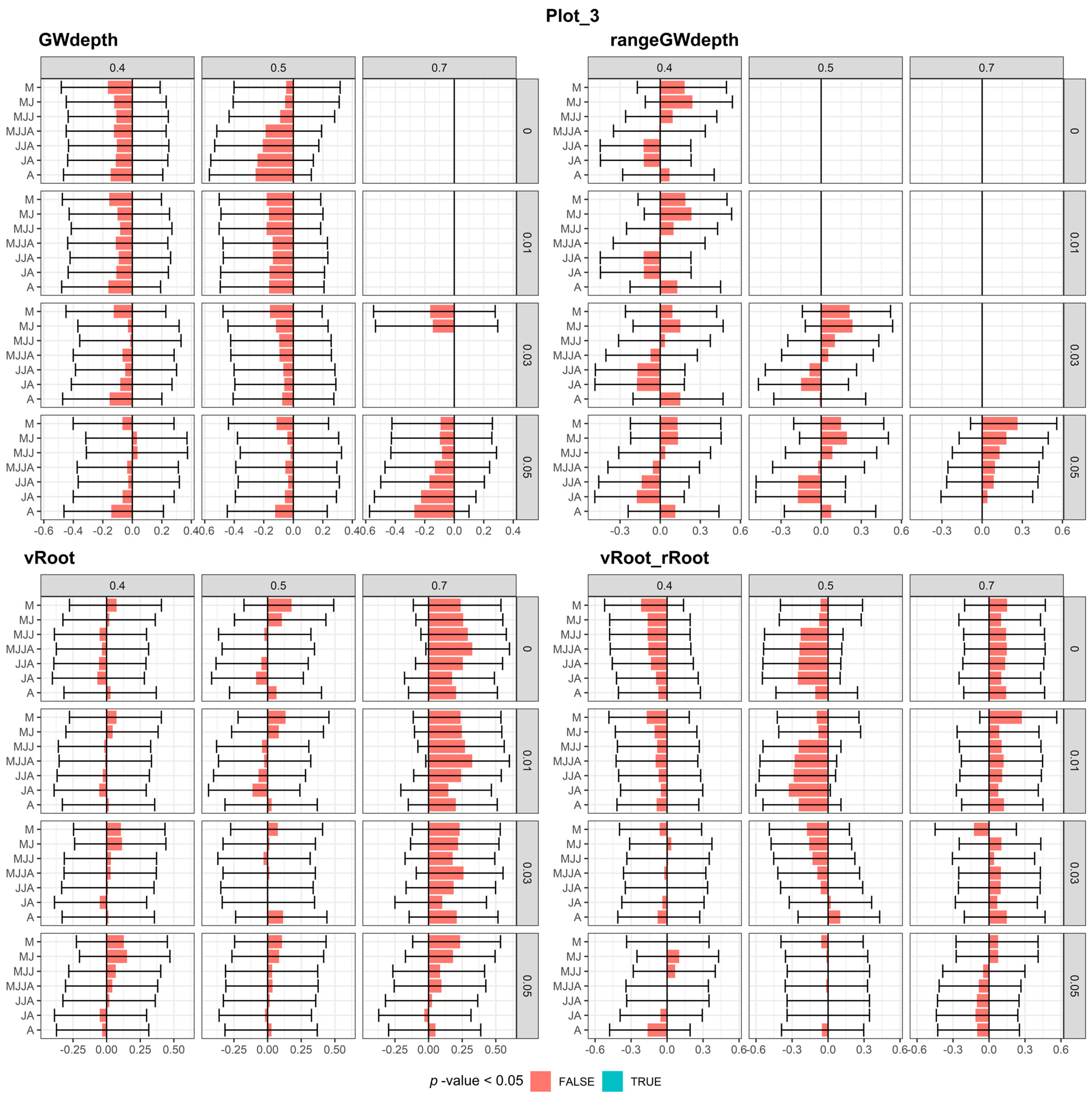
3.3.2. Modeled Soil Water Conditions

For Plot-1, the depth to the groundwater (GWdepth, Figure 10, Supplementary Materials Table S3) displayed a positive, but not significant, correlation for most of the model instances, i.e., deeper groundwater was correlated with better growing conditions. This correlation grew stronger for the summer months in the “driest” of the model instances. Interestingly, the range of depth to groundwater (rangeGWdepth) had a positive significant correlation with tree-ring increment for the spring months in the case of the “driest” model instances as well. This rangeGWdepth parameter could reflect the same phenomenon as the vRoot parameter: drawdown of the groundwater table due to root water uptake. The actual root water uptake (vRoot) displayed a significant positive correlation in May but a negative, but not significant, one later in the summer, suggesting that a higher transpiration water demand in spring as well as a lesser demand in summer favored tree growth. For this hydric site, this observation contradicted a more general finding that any positive effect on growth in early spring tends to be offset by drought stress in the summer [18]. The actual modeled root water uptake (vRoot), as well as the ratio between the potential and actual root water uptakes, had a positive and often significant correlation in spring and the beginning of summer. However, this correlation decreased for the later part of the summer. Notably, these correlations were generally stronger for dryer model instances (a higher LAI and lower groundwater exfiltration). These observations indicated the importance of meeting the transpiration water demand for the first half of the growing season in setting the growth trajectory for the rest of the season.

In the case of Plot-3, the tree-ring increment generally had an insignificant correlation with the modeled soil water parameters. However, its correlation with the depth to groundwater (GWdepth, Figure 11) was generally negative, i.e., deeper groundwater was not conductive to tree-ring growth. The range of the depth to the groundwater (rangeGWdepth) did not display a clear trend either. The potential root water uptake (rRoot) had a positive but insignificant correlation at the beginning of the growing season, indicating the importance of warm springs for facilitating growth. It could be noted that the highest positive correlation between tree-ring growth and actual water uptake was observed for model instances with the highest kLAI. The correlation between the tree-ring increment and the ratio between actual and potential root water uptake (vRoot_rRoot, Figure 11) varied among model instances, but was mostly neutral or negative, indicating that, if the modeled transpiration water demand was not met, (low vRoot and rRoot ratio), the respective tree-ring increment was wider.

Contrasting patterns of correlations between tree-ring increment and modeled soil water parameters were observed for Plot-1 and Plot-3. In the case of Plot-1, the correlation with meteorological parameters was insignificant, while the modeled actual root water uptake and the ratio between actual and potential root water uptake often had a significant positive correlation with the tree-ring increment. Meanwhile, in the case of Plot-3, the correlation with the meteorological parameters—mean temperature and precipitation—was positive and significant, while the correlation with the modeled soil water parameters was insignificant.

4. Discussion

We used one-dimensional soil water models to simulate water regimes at two hydric forest plots, informed by field observations and forced by an E-OBS gridded meteorological observation dataset. Twelve instances of each of the models were invoked by defining a range of active leaf area proportions (kLAI 0.4, 0.5 and 0.7) and groundwater exfiltration levels (water seep-in into soil profile; 0.00, 0.01, 0.03 and 0.05 cm day⁻¹). We showed that the considered ranges of these two parameters resulted in contrasting soil water regimes, ranging from desiccated to predominantly waterlogged soil conditions during the growing season. Major differences emerged when comparing the model output to local tree-ring chronologies for the two study sites.

The black alder is a wetland-adapted tree species with a two-tier root system, comprising a dense network of shallow, often adventitious, roots for nutrient extraction and well-developed taproots to access groundwater during times of soil water scarcity [61]. The roots are adapted to growing in oxygen-deprived soils. A high transpiration rate of the black alder has been observed, even when the topsoil water potential drops sharply and perennial vegetation wilts permanently, instead of regulating stomata conductance [62]; therefore, the transpiration remains high as long as there is water available in a relatively deep root zone. We observed tap roots at a depth of up to 1.3 m and small roots at a depth of up to 1.7 m. However, in our model, the rooting depth was limited to 1 m.

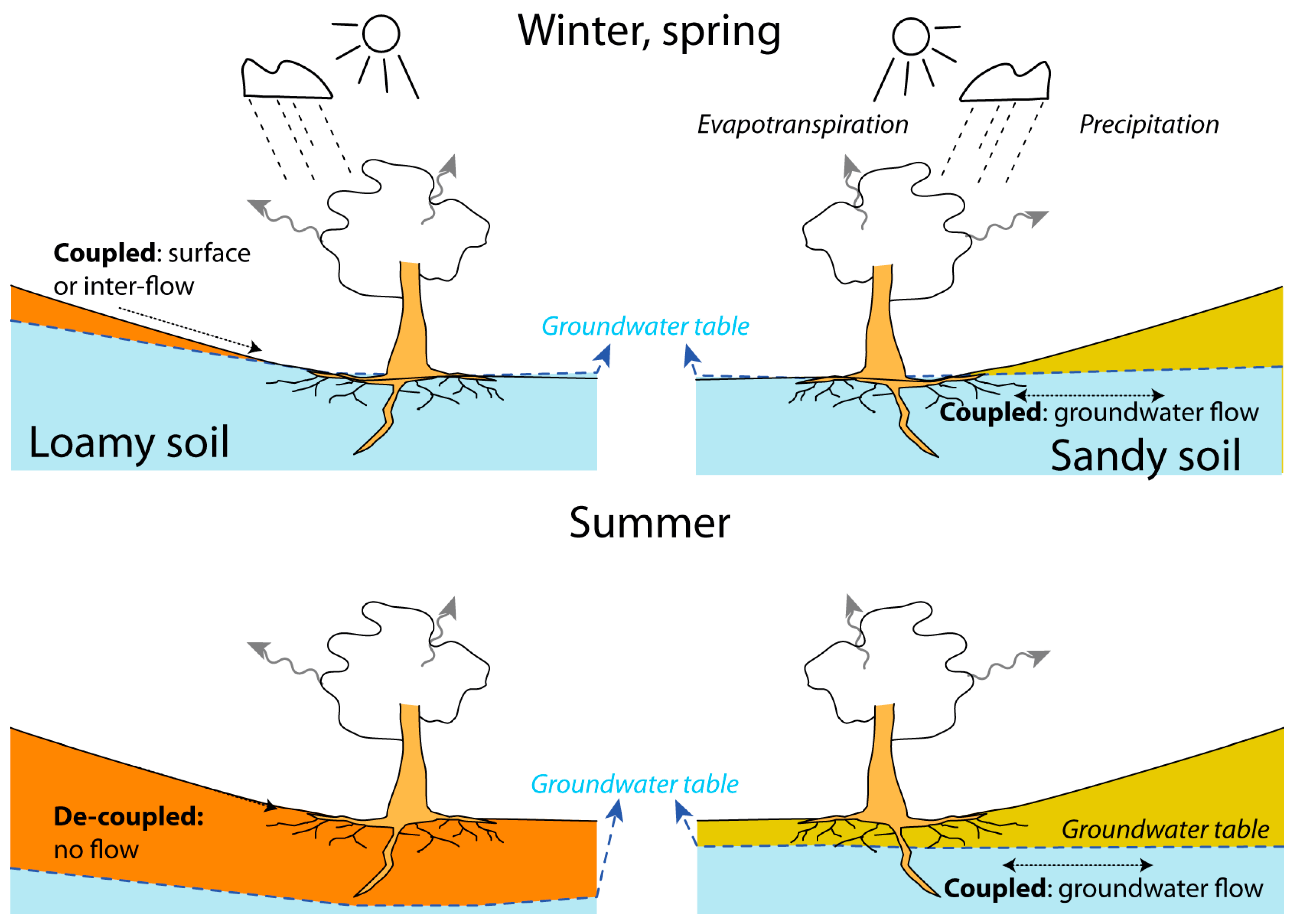
4.1. Hydrological Coupling and Decoupling

The model results indicate that, along with precipitation, significant additional water input is needed to maintain the observed soil water regime at the study sites (Figure 5 and Figure 6). The study sites are non-riparian wetland forests. Therefore, the additional water input must come in the form of surface run-on or groundwater exfiltration, sourced from surrounding slightly elevated (Figure 1) areas. Thus, it is possible to claim that the wetland forest areas—water receptors—are hydrologically coupled with the upland (water source) areas.

The two studied forest plots had a contrasting correlation pattern with the modeled soil water regime and yearly tree-ring increment. In Plot-1, on average, large fluctuations in the yearly groundwater level were observed and the higher modeled actual root water uptake in spring aligned with wider tree rings (Figure 10). It appeared that high root water uptake in spring determined the radial growth rate for the given year. In contrast, in Plot-3, the yearly groundwater fluctuations were smaller (Figure 7 and Figure 8) and no significant correlation between the models’ soil water parameters and tree rings was detected (Figure 11).

Contrasting conceptual models of the hydrological coupling between the elevated (water source) areas and the studied depression (water recipient) areas regarding additional water input for the two sites can be observed (Figure 12). Geomorphologically, the two sites were similar: shallow depressions on a forested plain. However, in Plot-1, the subsoil material was heavy silty clay loam, while, in Plot-3, it was loamy sand or sand (Table 2). The hydraulic conductivity as well as the plant-available water storage capacity of the subsoil material were much lower in Plot-1 than in Plot-3. It appeared that, during high-water periods from late autumn to spring, the run-off from surrounding areas entered Plot-1 as intermediate flow within the upper high-conductivity part of the soil profile. In contrast, the excess water entered Plot-3 as groundwater flow. During low-water seasons—summer and early autumn—the depression in Plot-1 was effectively hydrologically isolated (decoupled) from the surrounding elevated areas. Little to no horizontal soil or groundwater transfer between the depression and elevated areas can be expected. Meanwhile, in Plot-3, the groundwater flow can relatively freely redistribute water between macro-environments; depressions and elevated areas were hydrologically coupled. Thus, the differences between the two sites regarding the soil water regime emerged during summer.

The dynamics proposed in this paper are supported by the observed correlation pattern between hydro-meteorological parameters and local dendrochronology. At the start of the growing season, the increasing transpiration in surrounding elevated areas would drive down the groundwater table in both sites. For the water regime of Plot-1, it would have little to no effect, as the low-conductivity subsoil limited groundwater flow. Meanwhile, in Plot-3, the transpiration in surrounding elevated areas decreased the water table in hydric depressions as well, providing for better soil aeration and correspondingly enabling root water uptake. In Plot-3, the highest positive correlation of the tree-ring increment with the actual water uptake was observed for the two “driest” model instances (highest LAI and lowest water supply: P3_0.7_0.01_Seep_In and P3_0.7_0.00_Seep_In; (Figure 11)), which represented the conditions expected in the surrounding elevated areas. This is why we saw opposite correlations in Plot-1 and Plot-3 between the tree-ring increment and depth to groundwater and actual root water uptake (Figure 11 and Figure 12).

We propose that the subsoil’s hydrological properties determine whether hydric forest sites remain hydrologically coupled with the surrounding elevated water-source areas or become decoupled during the dry season. Hydric forests on clay-rich soils with low hydrological conductivity become effectively decoupled from the surrounding elevated areas, while hydric forests on sandy soils remain hydrologically coupled with the surrounding elevated areas by the groundwater flow. These differences determine how the sites react to meteorological conditions. The soil water regime in low-soil-conductivity sites is driven by the local balance between evapotranspiration, precipitation and soil water storage, while in sandy soil sites, the growing season’s water balance can become dominated by processes taking place in surrounding elevated areas. Although water transfer in the form of groundwater flow from upland areas to depressions is well established [90], this process can be a seasonal phenomenon in some locations and continuous in others as a function of the soil type.

4.2. Implications of the Hydrological Coupling/Decoupling

In the following paragraphs, we present several examples where the observed hydrological phenomena can be better understood by applying the concept of the hydrological coupling and decoupling of the topographic or hydrological elements of the landscape.

Perhaps an extreme example of a strongly coupled hydrological regime is the decadal water level fluctuations of the Kurtna Lake district in Estonia [91]. It was suggested that, at this site, the destruction and regrowth of a pine forest modified the balance between precipitation and transpiration, causing decadal fluctuation of the lake level by more than 3 m. The coupling between the lake level and the water balance of the surrounding hills was enabled by the sand and gravel subsoil material of the kame field. This would not be possible if the lake depressions and surrounding elevated areas were hydrologically decoupled.

In water-limited boreal environments and periods, the hydrological flow comes from the wetlands to the surrounding elevated areas due to the higher LAI and hence potential transpiration of the upland vegetation [14]. However, this flow can be significant only if the two systems are hydrologically coupled, i.e., if the subsoil hydraulic conductivity is sufficiently high to enable the transfer of meaningful volumes of water via groundwater flow. In the subsurface, the presence of a groundwater head gradient does not indicate water flow per se, rather the opposite: steep gradients develop in sites where there is limited flow, as, otherwise, the flow would smooth the gradient. Indeed, in the observed groundwater head, the gradient from wetland to upland was lowest in the sites with higher conductivity [14], indicating stronger coupling between hydrological elements of the landscape.

In settings with higher elevation differences and/or a heterogenous geological structure, the thresholds for seasonal hydrological coupling/decoupling might not be reached. Groundwater export from uplands can ensure continuous water supply to the wetlands in depressions despite strong (more than one order of magnitude) [92] discharge variability or changing water sources [93], where the tile drainage can be one of the most important run-off-forming components [94]. In such locations, continuous soil waterlogging can prevent the establishment of forest ecosystems. However, as this study has shown, if the groundwater exfiltration decreases below a certain threshold, forest transpiration can enable soil aeration and thus the establishment of a forest ecosystem. Thus, the seasonal hydrological decoupling of uplands and depressions is key for the establishment of forest ecosystems instead of peatlands [3].

Along with water, plant nutrients such as phosphorus and nitrogen are exported from elevated areas to depressions [95] (hydric sites). It can be expected that, during the periods when such depressions are flooded, plant roots grow into the water puddles, extracting nutrients directly from the water. It has been shown with maize (Zea mays) as the model species that even dryland plants are able to offset the detrimental effects caused by soil waterlogging by extracting nutrients directly from the water, with new adventitious effects [96]. Fine tree roots in temperate and boreal climates have a life span of mostly less than 5 years [97]; therefore, it can be expected that wetland-adapted plants such as black alder will opportunistically explore flooded environments to benefit from the extra nutrients flushed from water-source areas. In addition, root growth directly in the water can increase root water uptake and help drive down the water table in the beginning of the growing season, facilitating the establishment of aerated soil conditions.

The seasonal coupling and decoupling of hydric sites to and from upland sources have implications for the introduction of continuous-cover forestry as a forest soil management strategy in northern settings. In continuous-cover forestry, only a certain proportion of the trees are harvested in order to keep the transpiration of remaining trees sufficiently high, preventing soil waterlogging during the growing season and thus eliminating the need for the maintenance of drainage networks [9,10]. It can be speculated that, in hydric sites that become decoupled from water-source areas during the growing season, the effects of continuous-cover forestry would be much stronger than in other cases where such decoupling does not take place.

The proposed coupling of the hydrological regime is likely to act as a primary control on groundwater table dynamics, controlling most of the aspects of the groundwater level, such as amplitude, seasonality, inter-annual variability, boundedness and others [98]. The seasonal coupling/decoupling is an important aspect that needs to be considered when exploring the use of similarity-based approaches in predicting the seasonal dynamics of the groundwater head in ungauged locations [99]. The hydrological coupling/decoupling of different landscape elements acts as a primary control of the groundwater level’s seasonality; it is controlled by the subsoil’s hydrological properties, primarily its hydrological conductivity.

5. Conclusions

Wet conditions in hydric sites in hemiboreal lowland forests are often maintained via groundwater exfiltration or run-on from surrounding elevated areas and the water recipient hydric sites are hydrologically coupled to the water-source areas. We set up Hydrus-1D soil water models for two study sites and explored the model output for 12 instances with variable active proportions of leaf area and groundwater exfiltration rates. These two parameters could balance each other out, as the model yielded similar results with different parameter values. Furthermore, we compared the model output to the residual tree-ring chronology for the two study sites. It was found that at the clay soil site, the modeled root water uptake had a significant positive correlation with residual tree-ring chronology, while at the sandy soil site, tree-ring chronology had a stronger correlation with the meteorological conditions, namely precipitation and temperature. In addition, we can observe a trend towards dryer less waterlogged soil conditions, which ought to favor forest growth in these study locations.

We conceptualize that the water-source and -recipient sites can become decoupled during the dry season (when evapotranspiration is higher than precipitation) if the subsoil’s hydraulic conductivity is low, while they can remain coupled if the conductivity is high. Hydric forests on clay-rich soils with low hydrological conductivity become effectively decoupled from the surrounding elevated areas, while hydric forests on sandy soils remain hydrologically coupled with the surrounding elevated areas due to the groundwater flow. These differences determine how the sites react to meteorological conditions. The soil water regime in the low-soil-conductivity sites is driven by the local balance between evapotranspiration, precipitation and soil water storage, while in the sandy soil sites, the growing season’s water balance can potentially be dominated by processes taking place in surrounding elevated areas. This behavior is reflected in the soil water regime and the radial growth rate of the trees and can have implications for the forest management practices of these sites.

References

1. Forzieri, G.; Dakos, V.; McDowell, N.G.; Ramdane, A.; Cescatti, A. Emerging Signals of Declining Forest Resilience under Climate Change. Nature 2022, 608, 534–539. [Google Scholar] [CrossRef] [PubMed]
2. Reich, P.B.; Bermudez, R.; Montgomery, R.A.; Rich, R.L.; Rice, K.E.; Hobbie, S.E.; Stefanski, A. Even Modest Climate Change May Lead to Major Transitions in Boreal Forests. Nature 2022, 608, 540–545. [Google Scholar] [CrossRef] [PubMed]
3. van der Velde, Y.; Temme, A.J.A.M.; Nijp, J.J.; Braakhekke, M.C.; van Voorn, G.A.K.; Dekker, S.C.; Dolman, A.J.; Wallinga, J.; Devito, K.J.; Kettridge, N.; et al. Emerging Forest–Peatland Bistability and Resilience of European Peatland Carbon Stores. Proc. Natl. Acad. Sci. USA 2021, 118, e2101742118. [Google Scholar] [CrossRef]
4. Nave, L.E.; Gough, C.M.; Perry, C.H.; Hofmeister, K.L.; Le Moine, J.M.; Domke, G.M.; Swanston, C.W.; Nadelhoffer, K.J. Physiographic Factors Underlie Rates of Biomass Production during Succession in Great Lakes Forest Landscapes. For. Ecol. Manag. 2017, 397, 157–173. [Google Scholar] [CrossRef]
5. Mustroph, A.; Albrecht, G. Tolerance of Crop Plants to Oxygen Deficiency Stress: Fermentative Activity and Photosynthetic Capacity of Entire Seedlings under Hypoxia and Anoxia. Physiol. Plant. 2003, 117, 508–520. [Google Scholar] [CrossRef]
6. Mander, Ü.; Krasnova, A.; Schindler, T.; Megonigal, J.P.; Escuer-Gatius, J.; Espenberg, M.; Machacova, K.; Maddison, M.; Pärn, J.; Ranniku, R.; et al. Long-Term Dynamics of Soil, Tree Stem and Ecosystem Methane Fluxes in a Riparian Forest. Sci. Total Environ. 2022, 809, 151723. [Google Scholar] [CrossRef]
7. Evans, C.D.; Peacock, M.; Baird, A.J.; Artz, R.R.E.; Burden, A.; Callaghan, N.; Chapman, P.J.; Cooper, H.M.; Coyle, M.; Craig, E.; et al. Overriding Water Table Control on Managed Peatland Greenhouse Gas Emissions. Nature 2021, 593, 548–552. [Google Scholar] [CrossRef]
8. Zalitis, P.; Indriksons, A. The Hydrological Properties of Waterlogged and Drained Forests in Latvia. J. Water Land Dev. 2009, 13, 69–86. [Google Scholar] [CrossRef]
9. Nieminen, M.; Hökkä, H.; Laiho, R.; Juutinen, A.; Ahtikoski, A.; Pearson, M.; Kojola, S.; Sarkkola, S.; Launiainen, S.; Valkonen, S.; et al. Could Continuous Cover Forestry Be an Economically and Environmentally Feasible Management Option on Drained Boreal Peatlands? For. Ecol. Manag. 2018, 424, 78–84. [Google Scholar] [CrossRef]
10. Laudon, H.; Hasselquist, E.M. Applying Continuous-Cover Forestry on Drained Boreal Peatlands; Water Regulation, Biodiversity, Climate Benefits and Remaining Uncertainties. Trees For. People 2023, 11, 100363. [Google Scholar] [CrossRef]
11. Devito, K.J.; Hokanson, K.J.; Moore, P.A.; Kettridge, N.; Anderson, A.E.; Chasmer, L.; Hopkinson, C.; Lukenbach, M.C.; Mendoza, C.A.; Morissette, J.; et al. Landscape Controls on Long-Term Runoff in Subhumid Heterogeneous Boreal Plains Catchments. Hydrol. Process. 2017, 31, 2737–2751. [Google Scholar] [CrossRef]
12. Gribovszki, Z.; Kalicz, P.; Palocz-Andresen, M.; Szalay, D.; Varga, T. Hydrological Role of Central European Forests in Changing Climate –Review. Idojaras 2019, 123, 535–550. [Google Scholar] [CrossRef]
13. Tóth, J. A Theoretical Analysis of Groundwater Flow in Small Drainage Basins. J. Geophys. Res. 1963, 68, 4795–4812. [Google Scholar] [CrossRef]
14. Hokanson, K.J.; Peterson, E.S.; Devito, K.J.; Mendoza, C.A. Forestland-Peatland Hydrologic Connectivity in Water-Limited Environments: Hydraulic Gradients Often Oppose Topography. Environ. Res. Lett. 2020, 15, 034021. [Google Scholar] [CrossRef]
15. Komatsu, H.; Kume, T. Modeling of Evapotranspiration Changes with Forest Management Practices: A Genealogical Review. J. Hydrol. 2020, 585, 124835. [Google Scholar] [CrossRef]
16. Tor-ngern, P.; Oren, R.; Palmroth, S.; Novick, K.; Oishi, A.; Linder, S.; Ottosson-Löfvenius, M.; Näsholm, T. Water Balance of Pine Forests: Synthesis of New and Published Results. Agric. For. Meteorol. 2018, 259, 107–117. [Google Scholar] [CrossRef]
17. Finzi, A.C.; Giasson, M.A.; Barker Plotkin, A.A.; Aber, J.D.; Boose, E.R.; Davidson, E.A.; Dietze, M.C.; Ellison, A.M.; Frey, S.D.; Goldman, E.; et al. Carbon Budget of the Harvard Forest Long-Term Ecological Research Site: Pattern, Process, and Response to Global Change. Ecol. Monogr. 2020, 90, e01423. [Google Scholar] [CrossRef]
18. Dow, C.; Kim, A.Y.; D’Orangeville, L.; Gonzalez-Akre, E.B.; Helcoski, R.; Herrmann, V.; Harley, G.L.; Maxwell, J.T.; McGregor, I.R.; McShea, W.J.; et al. Warm Springs Alter Timing but Not Total Growth of Temperate Deciduous Trees. Nature 2022, 608, 552–557. [Google Scholar] [CrossRef]
19. Šimůnek, J.; Šejna, M.; Saitoh, T.M.; Sakai, M.; van Genuchten, M.T. The HYDRUS-1D Software Package for Simulating the One-Dimensional Movement of Water, Heat, and Multiple Solutes in Variably-Saturated Media. In University of California-Riverside Research Reports; University of California: Los Angeles, CA, USA, 2013; p. 343. [Google Scholar]
20. Kalvāns, A.; Dauškane, I. Data Set Supporting Publication “Seasonal Hydrological Coupling-Decoupling as a Key Element in Soil Water Regime of Hydric Forests” Submitted for the Journal of Hydrology by Kalvāns A. and Dauškāne I. [Data Set]. Zenodo 2023. [Google Scholar] [CrossRef]
21. LĢIA Digital Height Model Basic Data. Available online: https://www.lgia.gov.lv/en/Digitālaisvirsmasmodelis (accessed on 14 October 2021).
22. Jaagus, J.; Briede, A.; Rimkus, E.; Remm, K. Variability and Trends in Daily Minimum and Maximum Temperatures and in the Diurnal Temperature Range in Lithuania, Latvia and Estonia in 1951–2010. Theor. Appl. Climatol. 2014, 118, 57–68. [Google Scholar] [CrossRef]
23. Kalvāns, A.; Kalvāne, G.; Zandersons, V.; Gaile, D.; Briede, A. Recent Seasonally Contrasting and Persistent Recent Warming Trends in Latvia. Theor. Appl. Climatol. 2023. [Google Scholar] [CrossRef]
24. Jaagus, J.; Briede, A.; Rimkus, E.; Sepp, M. Changes in Precipitation Regime in the Baltic Countries in 1966–2015. Theor. Appl. Climatol. 2018, 131, 433–443. [Google Scholar] [CrossRef]
25. Jaagus, J.; Aasa, A.; Aniskevich, S.; Boincean, B.; Bojariu, R.; Briede, A.; Danilovich, I.; Castro, F.D.; Dumitrescu, A.; Labuda, M.; et al. Long-term Changes in Drought Indices in Eastern and Central Europe. Int. J. Climatol. 2022, 42, 225–249. [Google Scholar] [CrossRef]
26. Keith, D.A.; Ferrer-Paris, J.R.; Nicholson, E.; Bishop, M.J.; Polidoro, B.A.; Ramirez-Llodra, E.; Tozer, M.G.; Nel, J.L.; Mac Nally, R.; Gregr, E.J.; et al. A Function-Based Typology for Earth’s Ecosystems. Nature 2022, 610, 513–518. [Google Scholar] [CrossRef] [PubMed]
27. Keith, D.A.; Ferrer-paris, J.R.; Nicholson, E.; Kingsford, R.T. IUCN Global Ecosystem Typology 2.0: Descriptive Profiles for Biomes and Ecosystem Functional Groups; IUCN, International Union for Conservation of Nature: Gland, Switzerland, 2020; ISBN 9782831720777. [Google Scholar]
28. Burton, T.M. Swamps—Wooded Wetlands. Encycl. Inl. Waters 2009, 549–557. [Google Scholar] [CrossRef]
29. Misans, J.; Murnieks, A.; Strautnieks, I. Latvijas Geologiska Karte, Merogs 1:200000. 32.Lapa-Jelgava (Paskaidrojuma Teksts Un Kartes) (in Latvian) Latvian State Geological Fund No. 12444; 2001; Available online: https://www.meteo.lv/en/pakalpojumi/geologiska-un-hidrogeologiska-informacija/kartes/latvijas-geologiska-karte-kvartara-nogulumu-karte-meroga-1-200000?id=3339&cid=1037 (accessed on 24 August 2023).
30. Takčidi, E. Datu Bāzes “Urbumi” Dokumentācija [Documentation of the Database “Boreholes”]; State Geological Survey: Riga, Latvia, 1999. [Google Scholar]
31. Spalviņš, A.; Krauklis, K.; Aleksāns, O.; Lāce, I. Latvijas Hidroģeoloģiskā Modeļa LAMO Izveidošana, Izmantošana Un Pilnveidošana (Development, Application and Upgrading of the Hydrogeological Model of Latvia LAMO; in Latvian). Bound. Field Probl. Comput. Simul. 2018, 57, 5–14. [Google Scholar] [CrossRef]
32. Valtera, M.; Schaetzl, R.J. Pit-Mound Microrelief in Forest Soils: Review of Implications for Water Retention and Hydrologic Modelling. For. Ecol. Manag. 2017, 393, 40–51. [Google Scholar] [CrossRef]
33. Megonigal, J.P.; Patrick, W.H.; Faulkner, S.P. Wetland Identification in Seasonally Flooded Forest Soils: Soil Morphology and Redox Dynamics. Soil Sci. Soc. Am. J. 1993, 57, 140–149. [Google Scholar] [CrossRef]
34. Virbulis, J.; Bethers, U.; Saks, T.; Sennikovs, J.; Timuhins, A. Hydrogeological Model of the Baltic Artesian Basin. Hydrogeol. J. 2013, 21, 845–862. [Google Scholar] [CrossRef]
35. Monteith, J.L. Evaporation and Surface Temperature. Q. J. R. Meteorol. Soc. 1981, 107, 1–27. [Google Scholar] [CrossRef]
36. McMahon, T.A.; Peel, M.C.; Lowe, L.; Srikanthan, R.; McVicar, T.R. Estimating Actual, Potential, Reference Crop and Pan Evaporation Using Standard Meteorological Data: A Pragmatic Synthesis. Hydrol. Earth Syst. Sci. 2013, 17, 1331–1363. [Google Scholar] [CrossRef]
37. Zālītis, P. Mežs Un Ūdens; Laiviņš, M., Ed.; Latviajs Valsts mežzinātnes institūts “Silava”: Salaspils, Latvia, 2012; Volume 356, ISBN 9789934801662. [Google Scholar]
38. Kalvans, A. Run-on Contribution to the Soil Water Balance to the Temperate Forests. In Proceedings of the XXXI Nordic Hydrological Conference, Tallinn, Estonia, 15–18 August 2022. [Google Scholar]
39. Allen, R.G.; Pereira, L.S.; Raes, D.; Smith, M. Crop Evapotranspiration-Guidelines for Computing Crop Water Requirements-FAO Irrigation and Drainage Paper 56; FAO: Rome, Italy, 1998; ISBN 92-5-104219-5. [Google Scholar]
40. Wolfs, D.; Verger, A.; Van der Goten, R.; Sánchez-Zapero, J. Product User Manual Leaf Area Index (LAI), Fraction of Absorbed Photosynthetically Active Radiation (FAPAR) Fraction of Green Vegetation Cover (FCOVER) Collection 300m, version 1.1; VITO: Mol, Belgium, 2021. [Google Scholar]
41. Sutton, O.F.; Price, J.S. Soil Moisture Dynamics Modelling of a Reclaimed Upland in the Early Post-Construction Period. Sci. Total Environ. 2020, 718, 134628. [Google Scholar] [CrossRef]
42. Eijkelkamp. 09.02 Laboratory-Permeameters, Operating Instructions, Brand Data Laboratory Permeameter; Eijkelkamp: Giesbeek, The Netherlands, 2013; Available online: https://en.eijkelkamp.com/products/laboratory-equipment/soil-water-permeameters.html (accessed on 10 September 2022).
43. Schindler, U.; Durner, W.; von Unold, G.; Müller, L. Evaporation Method for Measuring Unsaturated Hydraulic Properties of Soils: Extending the Measurement Range. Soil Sci. Soc. Am. J. 2010, 74, 1071–1083. [Google Scholar] [CrossRef]
44. Schindler, U.; Durner, W.; von Unold, G.; Mueller, L.; Wieland, R. The Evaporation Method: Extending the Measurement Range of Soil Hydraulic Properties Using the Air-Entry Pressure of the Ceramic Cup. J. Plant Nutr. Soil Sci. 2010, 173, 563–572. [Google Scholar] [CrossRef]
45. van Genuchten, M. A Closed Form Equation for Predicting the Hydraulic Conductivity of Unsaturated Soils. Soil Sci. Soc. Am. J. 1980, 44, 892–898. [Google Scholar] [CrossRef]
46. Pertassek, T.; Peters, A.; Durner, W. HYPROP-FIT User’s Manual, version 3.1; METER Group AG: München, Germany, 2017; p. 66. [Google Scholar]
47. Cornes, R.C.; van der Schrier, G.; van den Besselaar, E.J.M.; Jones, P.D. An Ensemble Version of the E-OBS Temperature and Precipitation Data Sets. J. Geophys. Res. Atmos. 2018, 123, 9391–9409. [Google Scholar] [CrossRef]
48. Fan, Y.; Miguez-Macho, G.; Jobbágy, E.G.; Jackson, R.B.; Otero-Casal, C. Hydrologic Regulation of Plant Rooting Depth. Proc. Natl. Acad. Sci. USA 2017, 114, 10572–10577. [Google Scholar] [CrossRef]
49. Gale, M.R.; Grigal, D.F. Vertical Root Distributions of Northern Tree Species in Relation to Successional Status. Can. J. For. Res. 1987, 17, 829–834. [Google Scholar] [CrossRef]
50. Jackson, R.B.; Mooney, H.A.; Schulze, E.D. A Global Budget for Fine Root Biomass, Surface Area, and Nutrient Contents. Proc. Natl. Acad. Sci. USA 1997, 94, 7362–7366. [Google Scholar] [CrossRef] [PubMed]
51. Dos Santos, M.A.; De Jong Van Lier, Q.; Van Dam, J.C.; Bezerra, A.H.F. Benchmarking Test of Empirical Root Water Uptake Models. Hydrol. Earth Syst. Sci. 2017, 21, 473–493. [Google Scholar] [CrossRef]
52. Carminati, A.; Javaux, M. Soil Rather Than Xylem Vulnerability Controls Stomatal Response to Drought. Trends Plant Sci. 2020, 25, 868–880. [Google Scholar] [CrossRef] [PubMed]
53. Feddes, R.A.; Kowalik, P.; Kolinska-Malinka, K.; Zaradny, H. Simulation of Field Water Uptake by Plants Using a Soil Water Dependent Root Extraction Function. J. Hydrol. 1976, 31, 13–26. [Google Scholar] [CrossRef]
54. Jarvis, N.J. A Simple Empirical Model of Root Water Uptake. J. Hydrol. 1989, 107, 57–72. [Google Scholar] [CrossRef]
55. Jarvis, N.J. Simple Physics-Based Models of Compensatory Plant Water Uptake: Concepts and Eco-Hydrological Consequences. Hydrol. Earth Syst. Sci. 2011, 15, 3431–3446. [Google Scholar] [CrossRef]
56. Sutton, O.F.; Price, J.S. Modelling the Hydrologic Effects of Vegetation Growth on the Long-Term Trajectory of a Reclamation Watershed. Sci. Total Environ. 2020, 734, 139323. [Google Scholar] [CrossRef]
57. van Genuchten, M.T. A Numerical Model for Water and Solute Movement in and below the Root Zone; United States Department of Agriculture Agricultural Research Service US Salinity Laboratory: Riverside, CA, USA, 1987. [Google Scholar]
58. de Jong van Lier, Q.; van Dam, J.C.; Durigon, A.; dos Santos, M.A.; Metselaar, K. Modeling Water Potentials and Flows in the Soil-Plant System Comparing Hydraulic Resistances and Transpiration Reduction Functions. Vadose Zone J. 2013, 12, vzj2013.02.0039. [Google Scholar] [CrossRef]
59. Gong, D.; Kang, S.; Zhang, L.; Du, T.; Yao, L. A Two-Dimensional Model of Root Water Uptake for Single Apple Trees and Its Verification with Sap Flow and Soil Water Content Measurements. Agric. Water Manag. 2006, 83, 119–129. [Google Scholar] [CrossRef]
60. Green, S.R.; Vogeler, I.; Clothier, B.E.; Mills, T.M.; Dijssel, C. van den Modelling Water Uptake by a Mature Apple Tree. Soil Res. 2003, 41, 365. [Google Scholar] [CrossRef]
61. McVean, D.N. Ecology of Alnus glutinosa (L.) Gaertn: IV. Root System. J. Ecol. 1956, 44, 219. [Google Scholar] [CrossRef]
62. Eschenbach, C.; Kappen, L. Leaf Water Relations of Black Alder [Alnus glutinosa (L.) Gaertn.] Growing at Neighbouring Sites with Different Water Regimes. Trees 1999, 14, 28–38. [Google Scholar] [CrossRef]
63. Copernicus Global Land Service Leaf Area Index. Available online: https://land.copernicus.eu/global/products/lai (accessed on 14 February 2022).
64. Kalvāns, A.; Bitāne, M.; Kalvāne, G. Forecasting Plant Phenology: Evaluating the Phenological Models for Betula Pendula and Padus Racemosa Spring Phases, Latvia. Int. J. Biometeorol. 2015, 59, 165–179. [Google Scholar] [CrossRef] [PubMed]
65. Menzel, A.; Yuan, Y.; Matiu, M.; Sparks, T.; Scheifinger, H.; Gehrig, R.; Estrella, N. Climate Change Fingerprints in Recent European Plant Phenology. Glob. Change Biol. 2020, 26, 2599–2612. [Google Scholar] [CrossRef] [PubMed]
66. Kalvāne, G.; Kalvāns, A. Phenological Trends of Multi-Taxonomic Groups in Latvia, 1970–2018. Int. J. Biometeorol. 2021, 65, 895–904. [Google Scholar] [CrossRef] [PubMed]
67. Laube, J.; Sparks, T.H.; Estrella, N.; Menzel, A. Does Humidity Trigger Tree Phenology? Proposal for an Air Humidity Based Framework for Bud Development in Spring. New Phytol. 2014, 202, 350–355. [Google Scholar] [CrossRef] [PubMed]
68. Delpierre, N.; Dufrêne, E.; Soudani, K.; Ulrich, E.; Cecchini, S.; Boé, J.; François, C. Modelling Interannual and Spatial Variability of Leaf Senescence for Three Deciduous Tree Species in France. Agric. For. Meteorol. 2009, 149, 938–948. [Google Scholar] [CrossRef]
69. Fracheboud, Y.; Luquez, V.; Bjorken, L.; Sjodin, A.; Tuominen, H.; Jansson, S. The Control of Autumn Senescence in European Aspen. Plant Physiol. 2009, 149, 1982–1991. [Google Scholar] [CrossRef]
70. Zani, D.; Crowther, T.W.; Mo, L.; Renner, S.S.; Zohner, C.M. Increased Growing-Season Productivity Drives Earlier Autumn Leaf Senescence in Temperate Trees. Science 2020, 370, 1066–1071. [Google Scholar] [CrossRef]
71. Kumar, R.; Bishop, E.; Bridges, W.C.; Tharayil, N.; Sekhon, R.S. Sugar Partitioning and Source–Sink Interaction Are Key Determinants of Leaf Senescence in Maize. Plant Cell Environ. 2019, 42, 2597–2611. [Google Scholar] [CrossRef]
72. Herms, D. Using Degree-Days and Plant Phenology to Predict Pest Activity. In IPM (Integrated Pest Management) of Midwest Landscapes; Krischik, V., Davidson, J., Eds.; Minnesota Agricultural Experiment Station Publication: Saint Paul, MN, USA, 2004; pp. 49–59. [Google Scholar]
73. Smets, B.; Sánchez-Zapero, J. Vegetation and Energy, Product User Manual, Surface Albedo, Collection 1km, Version 1; VITO: Mol, Belgium, 2018; Volume 93. [Google Scholar]
74. Copernicus Global Land Service. Surface Albedo. 2020. Available online: https://land.copernicus.eu/global/products/sa (accessed on 9 September 2022).
75. Van Dijk, A.I.J.M.; Gash, J.H.; Van Gorsel, E.; Blanken, P.D.; Cescatti, A.; Emmel, C.; Gielen, B.; Harman, I.N.; Kiely, G.; Merbold, L.; et al. Rainfall Interception and the Coupled Surface Water and Energy Balance. Agric. For. Meteorol. 2015, 214, 402–415. [Google Scholar] [CrossRef]
76. van Dam, J.C.; Huygen, J.; Wesseling, J.G.; Feddes, R.A.; Kabat, P.; van Walsum, P.E.V.; Groenendijk, P.; van Diepen, C.A. Theory of SWAP version 2.0 Simulation of water flow, solute transport and plant growth in the Soil-Water-Atmosphere-Plant environment. Report 71; Department Water Resources, Wageningen Agricultural University: Wageningen, The Netherlands, 1997. [Google Scholar]
77. Šípek, V.; Hnilica, J.; Vlček, L.; Hnilicová, S.; Tesař, M. Influence of Vegetation Type and Soil Properties on Soil Water Dynamics in the Šumava Mountains (Southern Bohemia). J. Hydrol. 2020, 582, 124285. [Google Scholar] [CrossRef]
78. Dohnal, M.; Černý, T.; Votrubová, J.; Tesař, M. Rainfall Interception and Spatial Variability of Throughfall in Spruce Stand. J. Hydrol. Hydromech. 2014, 62, 277–284. [Google Scholar] [CrossRef]
79. Grissino-Mayer, H. A Manual and Tutorial for the Proper Use of an Increment Borer. Tree-Ring Res. 2003, 59, 63–79. [Google Scholar]
80. Rinn, F. TSAP-Win: Time Series Analysis and Presentation for Dendrochronology and Related Applications, version 0.55; User Reference: Heidelberg, Germany, 2003. [Google Scholar]
81. Holmes, R.L. Computer-Assisted Quality Control in Tree-Ring Dating and Measurement. Tree-Ring Bull. 1983, 43, 69–78. [Google Scholar]
82. Bunn, A.G. A Dendrochronology Program Library in R (DplR). Dendrochronologia 2008, 26, 115–124. [Google Scholar] [CrossRef]
83. R Development Core Team. R: A Language and Environment for Statistical Computing; R Foundation for Statistical Computing: Vienna, Austria, 2011; Volume 1, p. 409. [Google Scholar]
84. Holmes, R.L. Dendrochronology Program Library (DPL) Users Manual; The University of Arizona: Tuscon, Arizona, 1999. [Google Scholar]
85. R Core Team. R: A Language and Environment for Statistical Computing; R Foundation for Statistical Computing: Vienna, Austria, 2021. [Google Scholar]
86. Laganis, J.; Pečkov, A.; Debeljak, M. Modeling Radial Growth Increment of Black Alder (Alnus glutionsa (L.) Gaertn.) Tree. Ecol. Model. 2008, 215, 180–189. [Google Scholar] [CrossRef]
87. Babre, A.; Kalvāns, A.; Avotniece, Z.; Retiķe, I.; Bikše, J.; Jemeljanova, M.; Popovs, K.; Zelenkevičs, A.; Dēliņa, A. The Use of Predefined Drought Indices for the Assessment of Groundwater Drought Episodes in the Baltic States over the Period 1989–2018. J. Hydrol. Reg. Stud. 2022, 40, 101049. [Google Scholar] [CrossRef]
88. Schnabel, F.; Purrucker, S.; Schmitt, L.; Engelmann, R.A.; Kahl, A.; Richter, R.; Seele, C.; Skiadaresis, G.; Wirth, C. Cumulative Growth and Stress Responses to the 2018–2019 Drought in a European Floodplain Forest. Glob. Change Biol. 2022, 28, 1870–1883. [Google Scholar] [CrossRef]
89. Skaggs, R.W.; Amatya, D.M.; Chescheir, G.M. Effects of Drainage for Silviculture on Wetland Hydrology. Wetlands 2020, 40, 47–64. [Google Scholar] [CrossRef]
90. Miguez-Macho, G.; Fan, Y. Spatiotemporal Origin of Soil Water Taken up by Vegetation. Nature 2021, 598, 624–628. [Google Scholar] [CrossRef]
91. Vainu, M.; Terasmaa, J. Changes in Climate, Catchment Vegetation and Hydrogeology as the Causes of Dramatic Lake-Level Fluctuations in the Kurtna Lake District, NE Estonia. Est. J. Earth Sci. 2014, 63, 45–61. [Google Scholar] [CrossRef]
92. Kalvāns, A.; Popovs, K.; Priede, A.; Koit, O.; Retiķe, I.; Bikše, J.; Dēliņa, A.; Babre, A. Nitrate Vulnerability of Karst Aquifers and Associated Groundwater-Dependent Ecosystems in the Baltic Region. Environ. Earth Sci. 2021, 80, 628. [Google Scholar] [CrossRef]
93. Koit, O.; Tarros, S.; Pärn, J.; Küttim, M.; Abreldaal, P.; Sisask, K.; Vainu, M.; Terasmaa, J.; Retike, I.; Polikarpus, M. Contribution of Local Factors to the Status of a Groundwater Dependent Terrestrial Ecosystem in the Transboundary Gauja-Koiva River Basin, North-Eastern Europe. J. Hydrol. 2021, 600, 126656. [Google Scholar] [CrossRef]
94. Van Stempvoort, D.R.; MacKay, D.R.; Koehler, G.; Collins, P.; Brown, S.J. Subsurface Hydrology of Tile-drained Headwater Catchments: Compatibility of Concepts and Hydrochemistry. Hydrol. Process. 2021, 35, e14342. [Google Scholar] [CrossRef]
95. Liu, Y.; Du, J.; Xu, X.; Kardol, P.; Hu, D. Microtopography-Induced Ecohydrological Effects Alter Plant Community Structure. Geoderma 2020, 362, 114119. [Google Scholar] [CrossRef]
96. Kalvāns, A.; Kalvāne, G. Soil Waterlogging Stress Compensated by Root System Adaptation in a Pot Experiment with Sweet Corn Zea Mays Var. Saccharate. In Proceedings of the 22nd International Multidisciplinary Scientific GeoConference SGEM 2022, Issue, 3.1. Albena, Bulgaria, 4–10 June 2022; Trofymchuk, O., Rivza, B., Eds.; STEF92 Technology: Vienna, Austria, 2022; pp. 167–178. [Google Scholar]
97. Solly, E.F.; Brunner, I.; Helmisaari, H.S.; Herzog, C.; Leppälammi-Kujansuu, J.; Schöning, I.; Schrumpf, M.; Schweingruber, F.H.; Trumbore, S.E.; Hagedorn, F. Unravelling the Age of Fine Roots of Temperate and Boreal Forests. Nat. Commun. 2018, 9, 3006. [Google Scholar] [CrossRef]
98. Haaf, E.; Giese, M.; Heudorfer, B.; Stahl, K.; Barthel, R. Physiographic and Climatic Controls on Regional Groundwater Dynamics. Water Resour. Res. 2020, 56, e2019WR026545. [Google Scholar] [CrossRef]
99. Barthel, R.; Haaf, E.; Giese, M.; Nygren, M.; Heudorfer, B.; Stahl, K. Similarity-Based Approaches in Hydrogeology: Proposal of a New Concept for Data-Scarce Groundwater Resource Characterization and Prediction. Hydrogeol. J. 2021, 29, 1693–1709. [Google Scholar] [CrossRef]
Figure 1. Study site locations, overview map from European Commission, Eurostat (EuroGeographics), digital elevation model [21] derived from lidar data.
Forests 14 01734 g001
Figure 2. Simulated and observed [40] gap-filed yearly LAI trajectories for the two study sites.
Forests 14 01734 g002
Figure 3. Comparison between observed [40] gap-filed (LAI_proba) and model (LAI_model) LAI for the two study sites.
Forests 14 01734 g003
Figure 4. Tree-ring chronology for the study sites Plot-1 and Plot-2, where N stands for sample depth (number of trees); the tree ring index is the residual chronology (detrended tree-ring chronology) and the ring width is the individual tree-ring width (grey lines) and mean chronology (thick black line).
Forests 14 01734 g004
Figure 5. Modeled and observed depth to groundwater at the study site Plot-1 for the 12 model scenarios. Horizontally spaced facets represent the kLAI (proportion of active LAI); vertically spaced facets are the rate of groundwater exfiltration (cm day−1).
Forests 14 01734 g005
Figure 6. Modeled and observed depth to groundwater at the study site Plot-3 for the 12 model scenarios. Horizontally spaced facets represent the kLAI (proportion of active LAI); vertically spaced facets are the rate of groundwater exfiltration (cm day−1).
Forests 14 01734 g006
Figure 7. Simulated depth to groundwater for Plot-3. Note that a depth to groundwater greater than 240 cm is not shown.
Forests 14 01734 g007
Figure 8. Simulated depth to groundwater Plot-3. Note that a depth to groundwater greater than 240 cm is not shown.
Forests 14 01734 g008
Figure 9. Pearson correlations between the mean meteorological parameters and the residual tree-ring chronology: Wind—wind speed (km/day); Temp—air temperature (°C); Rad—solar radiation (MJ m−1 day−1); Prec—precipitation (cm); M—May; MJ—May–June; MJJ—May–July; MJJA—May–August; JJA—June–August; JA—July–August; A—August. The horizontal error bars represent the 95% confidence interval for the correlation coefficient and the green bars are correlation significant at 0.05 level.
Forests 14 01734 g009
Figure 10. Correlation matrix between modeled monthly soil and groundwater parameters and tree-ring residual chronology for the study site Plot-1: GWdepth—mean depth to groundwater (cm); rangeGWdepth—difference between maximal minimal GWdepth (cm); vRoot—modeled mean actual root water uptake (cm day−1); vRoot_rRoot—ratio between modeled mean actual and potential root water uptake; M—May; MJ—May–June; MJJ—May–July; MJJA—May–August; JJA—June–August; JA—July–August; A—August. The horizontal error bars represent the 95% confidence interval for the correlation coefficient and the green bars are correlation significant at 0.05 level. Missing data are model instances where fewer than 20 observations of the parameter were available. Missing data are model instances where, for more than 20 years, depth to groundwater (GWdepth) was not estimated, as the water potential at a 240 cm depth was less than 0.
Forests 14 01734 g010
Figure 11. Correlation matrix between modeled monthly soil and groundwater parameters and tree-ring residual chronology for the study site Plot-3: GWdepth—mean depth to groundwater (cm); rangeGWdepth—difference between maximal minimal GWdepth (cm); vRoot—modeled mean actual root water uptake (cm day−1); vRoot_rRoot—ratio between modeled mean actual and potential root water uptake; M—May; MJ—May–June; MJJ—May–July; MJJA—May–August; JJA—June–August; JA—July–August; A—August. The horizontal error bars represent the 95% confidence interval for the correlation coefficient and the green bars are correlation significant at 0.05 level.
Forests 14 01734 g011
Figure 12. The conceptual model of the hydrological coupling/decoupling of water donor (elevated areas) and water recipient (terrain depressions) areas. During the winter, water flows from elevated areas to depressions, but in summer, at sites with low-permeability clay soils, no water transfer between landscape domains takes place. However, in the high-permeability sand-soil sites, water is continuously redistributed between landscape domains.
Forests 14 01734 g012