Effects of Distance and Neighbor Size on Abies hickelii: The Asymmetric Competition Is Aggravated in an Endangered Species

Abstract

One of the hypotheses in the field of forest ecology suggests that competition among individual plants is asymmetric or unidirectional. This notion holds particular significance for endangered species, necessitating a comprehensive assessment of the impact of their closest competitors to understand their spatial distribution and local-scale interactions. The mean response of Abies hickelii’s diameter at breast height and total height was determined for each unit that increased the distance from its neighbor and each unit that changed the size of its neighbor. The results obtained through the analysis of covariance suggest that, for each meter that the distance from the neighbor increases, there is a mean gain of 1.13 cm in the diameter of the individuals studied. The height results showed higher sensitivity to changes in the neighbor distance than the diameter. It was observed that the population is exposed to asymmetric competition, suggesting that larger individuals take available resources disproportionately, thereby inhibiting the growth of smaller individuals. The intraspecific competition surpassed the interspecific competition. A suggestion was made to use selective thinning during the early-growth stages of the species. The habitat of the species studied is under strong pressure from land use change due to clandestine logging, the opening of roads, and other anthropogenic effects. Thus, these results represent an important step in the implementation of action strategies to preserve the species in the wild.

1. Introduction

Abies hickelii (Flous et Gaussen) is a critically endangered species found in isolated populations forming strips or small patches in the mountain ranges of Mexico, mainly in Chiapas, Oaxaca, and Veracruz [1]. Currently, it is listed in the endangered category on the IUCN Red List, and its population is decreasing [2,3]. This species has also been recognized as a priority for conservation in the official Mexican standard NOM-059-SEMARNAT-2010 related to the conservation of the diversity of species in wildlife (NOM-059, 2010). Small and isolated populations like A. hickelii are particularly vulnerable to competition for limited resources, which can be exacerbated by their low genetic diversity and increased inbreeding [4,5]. These factors hinder the species’ adaptive capacity and restrict its ability to expand its territory or thrive in the wild. Considering the context of climate change and land use alterations, understanding the factors influencing the growth and survival of geographically restricted populations like A. hickelii becomes vital for effective conservation efforts [6,7].

Understanding the pattern of spatial distribution of plants in wildlife in accurate and meaningful terms has not been an easy task due to various factors, including interactions such as competition and interference [8]. Conventionally, the effect of competition is usually assessed by looking at the average plant yield as a function of the density [9,10,11,12]. This approach, nevertheless, does not fully reveal the phenomenon of competition due to the effects associated with spatial and temporal variation in the natural environment, plant immobility, and phenotypic plasticity, among other aspects that are difficult to control [11]. An alternative approach to describing the structure, composition, and evolution of populations is studying plants at the individual level [11]; that is, assuming that a particular individual responds to the competitive activity of only some of its neighbors to a greater extent and not to the density of the entire population, this is understood as the joint effect of the total spatial relationships of the individuals [9,11,13].

In evaluating individual plant performance as a function of the observable neighbor characteristics, it is desirable to know the recent performance of the plant when neighbor conditions were not very different from the present [9]. Yet, if the individual performance history is unavailable due to ongoing variations in measurable neighbor characteristics, conducting a correlational study between the dimensions of specific reference trees and the size and proximity of their neighboring plants can offer valuable insights into plant interactions at the individual scale. In that sense, the total height and diameter at breast height are quintessential indicators of tree growth and resource utilization [14]. In this study, the rates of change in height and diameter at breast height of Abies hickelii were quantified as the unit changes in the distance and size of the five nearest neighbors. The study was guided by the following research questions: Do the size and proximity of neighbors, whether large or small, affect the reference trees? If yes, by how much are they affected? Which growth dimension, vertical or horizontal, is more influenced by the size and distance of the nearest competitors? Is the impact of neighbors when they belong to the same species similar to when they belong to different species? Answering these questions strengthens knowledge about the interactions occurring in the A. hickelii population at the local scale, which could be used to support the development of models of structure in future studies of forest dynamics and decisions related to the conservation of the species.

2. Materials and Methods

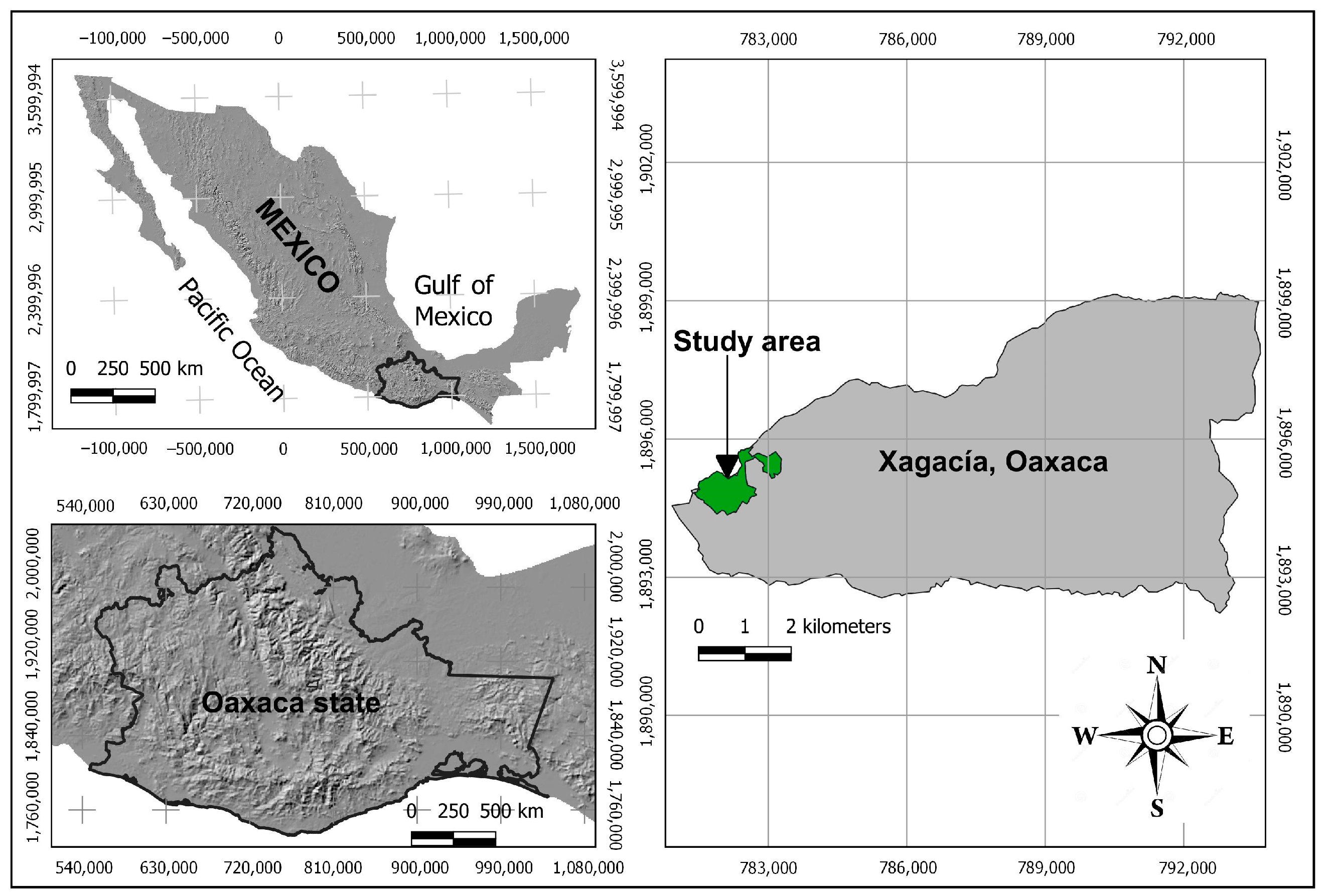
2.1. Sampling Area and Data Collection

The studied population of A. hickelii is located within the municipality of Santo Domingo Xagacía, in the vicinity of the mountain range known as Sierra Norte de Oaxaca, in southeastern Mexico, between the coordinates 96°21′01″ W and 17°07′04″ N and 96°20′44″ W, 17°07′43″ N (Datum: WGS84). The study area is approximately 112.27 hectares in size, and it is between 2810 and 3087 m above sea level. Our own estimates using historical climatic layers from 1961 to 1990 show that the mean annual temperature is between 10.3 and 11.9 °C and the mean annual precipitation is between 1301 and 1398 mm. During the months of the greatest vegetative activity (April–September), the average precipitation varies from 1045 to 11,104 mm, and the mean temperature ranges from 10.85 to 12.58 °C. The species observed in the study area during field data collection were mainly from the genera Pinus and Quercus, mainly P. ayacahuite Ehren, P. patula Schiede ex Schltdl, & Cham, P. pseudostrobus Lindl., Q. laurina Humb et Bonpl., Q. glabrescens A.Kern, and Q. obtusata Bonpl. (Figure 1).

2.2. Sampling and Data Collection

Nine sampling units were formed in the research area using cluster sampling, each covering an area of 10,000 m² with a radius of 56.42 m. Special attention was given to ensure coverage of the diverse local conditions present in the target area. This included variations in the terrain slope, geographic exposure, proximity to streams, and density. Areas heavily impacted by anthropogenic activities such as timber harvesting, agriculture, and roads were excluded from the sampling process.

Within each cluster, there were four circular plots, each measuring 400 m² in size with a radius of 11.28 m. These plots were strategically placed to achieve representative sampling. The first plot was established at the center of the main unit. Subsequently, the second, third, and fourth plots were positioned on the perimeter of the main plot, corresponding to azimuth angles of 0°, 120°, and 240° relative to magnetic north (north is indicated by a compass).

During data collection in each plot, various measurements were recorded. The average slope of the terrain, expressed as a percentage, was measured using a Suunto^® clinometer (model KB-14 Vantaa, Finland). Additionally, the orientation of the slope or geographic exposure was recorded in degrees ranging from 0 to 360°, with reference to magnetic north, using a compass. Furthermore, the elevation above sea level was captured using a GPS receiver.

In the 400 m² plots, an inventory of individuals of A. hickelii with a diameter at breast height (DBH) equal to or greater than 7.5 cm was conducted. In each of these plots, trees of the species of interest with the smallest and largest DBH were identified and designated as reference trees. Subsequently, the five nearest neighbors were located for each reference tree (RT) with a DBH greater than or equal to 7.5 cm, regardless of the species. It should be noted that some plots had no A. hickelii individuals, did not meet the criterion, or there were fewer than five neighbors (ATs) in the entire plot. For this reason, 57 reference trees and 269 neighboring trees were identified and georeferenced. Assuming that only the nearest competitors have the strongest influence on the reference trees [11], only the effect of the first five neighbors was evaluated here. This value (5) is close to 6 (k = 6), as suggested in the forestry literature for sampling [15,16]; also, it coincides with the minimum number of observations in which statistical efficiency was observed in a teak plantation study [17].

We recorded the linear distance (in meters) from the base of the RT stem to the base of the stem for each of the five defined neighbors. Additionally, we noted the location of each neighbor in degrees with respect to magnetic north, ranging from azimuth angles of 0 to 360°. For each of the RT and their five neighbors, we measured the DBH and total height (TH) (

Table 1. Summary of the descriptive statistics of the diameter at breast height of the reference trees (DBH-RT) and their first five neighbors (DBH-AT) and the total height of the reference trees (TH-RT) and their first five neighbors (TH-AT).

	DBH-AT	TH-AT	DBH-RT	TH-RT
Minimum	1.66	4.10	7.50	4.45
Maximum	119.60	46.00	75.05	42.50
Mean	24.66	16.73	23.27	16.74
Standard deviation	20.20	9.92	19.41	10.62
Asymmetry coefficient	1.49	1.00	1.10	1.09

).

2.3. Data Analysis

To assess whether the five nearest neighbors of A. hickelii were randomly distributed around the reference trees, two analyses were conducted. Firstly, the observed frequency of neighbors around each RT was subjected to the Wald–Wolfowitz randomization test using the “runs.test” function from the “randtests” package in the statistical software R v.3.6.1 [18]. Then, the confidence intervals of the empirical proportions were compared.

To analyze the distribution of neighbors around each RT, the contour of each tree was divided into eight quadrants based on the azimuth, proceeding clockwise: north (337.5–22.5°), northeast (22.5–67.5°), east (67.5–112.5°), southeast (112.5–157.5°), south (157.5–202.5°), southwest (202.5–247.5°), west (247.5–292.5°), and northwest (292.5–337.5°).

The observed proportions for each quadrant were estimated, and their corresponding 95% confidence intervals were calculated. To determine significant differences in the neighbor proportions between quadrants, overlapping intervals were considered to be non-significant, while non-overlapping intervals indicated significant differences. The confidence intervals were calculated using the Clopper–Pearson method [19] with the “DescTools” package in R v.3.6.1 [20]. A Bonferroni correction was applied by dividing the significance level (0.05) by the total number of comparisons (8).

To assess how changes in the distance and neighbor size (independent variables) affect the diameter and height of the TRs (variables of interest), we employed an analysis of covariance. This method incorporated, as a covariate, the groups of the five nearest competitors, determined by their sizes. The first group consisted of trees with a diameter at breast height (DBH) larger than those of any of their neighbors. The second subset included trees with a DBH smaller than those of any of their neighbors. The third comprised trees with the tallest overall height compared to their neighboring trees. Lastly, the fourth subset encompassed trees with a shorter total height than their competitors.

First, the hypothesis of null incidence of the groups in the predictor-variables-of-interest relationship was tested. Then, the rates of change in diameter and height of the reference trees were examined for each unit that the predictors increased or decreased.

To measure the impact of neighbors based on their size, we calculated the ratios of change in the diameter at breast height (DBH) and total height (TH) of the target trees for each unit of the relative size measure. Two measures of relative size were defined for this purpose: (i) the average relative size of the stem diameter at 1.3 m (RSD), which indicates the number of times the DBH of the neighboring tree was larger or smaller than that of the RT. In the results section, this measure is known as the horizontal relative size; (ii) the average relative size of the total height (RSH), which indicates the number of times the total height of the neighbor is larger or smaller than that of the RT. In the results section, this is known as the vertical relative size.

The relative size measure was obtained by dividing the corresponding size of the RT by the size of each neighbor. If the neighbor had larger dimensions, the quotient was a proper fraction (0–1). If the neighbor had smaller dimensions than the RT, the resulting quotient was an improper fraction (>1). To determine the predictor that exerted a more significant impact compared to its counterpart, a second iteration of the models was performed by scaling the original variables. This involved subtracting the mean from each value and dividing it by the standard deviation. By employing this scaling technique, the resulting rate of change accurately reflected the effect size of the predictor, independently of the unit of measurement. A larger standardized coefficient indicated a larger effect, while a smaller coefficient indicated a smaller effect. When calculating the coefficients, any value that produced a substantial bias was disregarded.

All models were evaluated by observing the percentage of variability that a predictor was able to explain (R²); likewise, the significant contribution of the regressor in the model was observed. For the latter, no a priori significance level was established. If the probability values associated with the coefficients were significantly close to zero, it suggested that the predictor contributed significantly to the variation in the response variable, since the evidence for the null contribution hypothesis was very low [21].

To determine the effect size due to neighboring species, Cohen’s standardized mean difference was used, which was calculated using the “cohen.d” function of the R package “effsize” [22]. For this purpose, the variables of interest were grouped into two subsets: (1) the first group corresponded to trees whose neighbors were only A. hickelii, and (2) the second group corresponded to trees whose neighbors were trees of species other than A. hickelii. Cohen’s d formula is expressed as follows:

$$d=\frac{(x_1-x_2)}{\sqrt{\frac{(n_1-1)S_1^2+(n_2-1)S_2^2}{n_1+n_2-2}}}$$

where x₁ and x₂ are the means of group 1 (A. hickelii) and group 2 (other species), respectively, and S1 and S2 are the variance of group 1 and group 2, respectively.

In an additional analysis, the distances of the five neighbors were modeled with the Weibull function. Parameter estimation was performed through the log-likelihood method by the Nelder–Mead algorithm [23] in R v.3.6.1. The expression of the Weibull probability density function, as reported by Prodan et al. [24], is expressed as:

$$f\left(x|c,b,a\right)=\frac{c}{b}{\left(\frac{x-a}{b}\right)}^{c-1}{e}^{\left(-{\left(\frac{x-a}{b}\right)}^c\right)}$$

and its cumulative function is:

$$F\left(x|c,b,a\right)=1-e^{\left(-{\left(\frac{x-a}{b}\right)}^c\right)}$$

Assuming that the maximum height of the density curve (peak) suggests the value of the modeled variable at which the maximum probability occurs, in this work, the formula employed to calculate the distance at which the probability of locating a neighbor is maximized was as follows:

$$max=a+b{\times }^{\left(1-{\left(1-\frac{1}{c}\right)}^{\frac{1}{c}}\right)}$$

In these formulas, c > 0 is the shape parameter, b > 0 is the scale parameter, and a > 0 is the location parameter.

3. Results

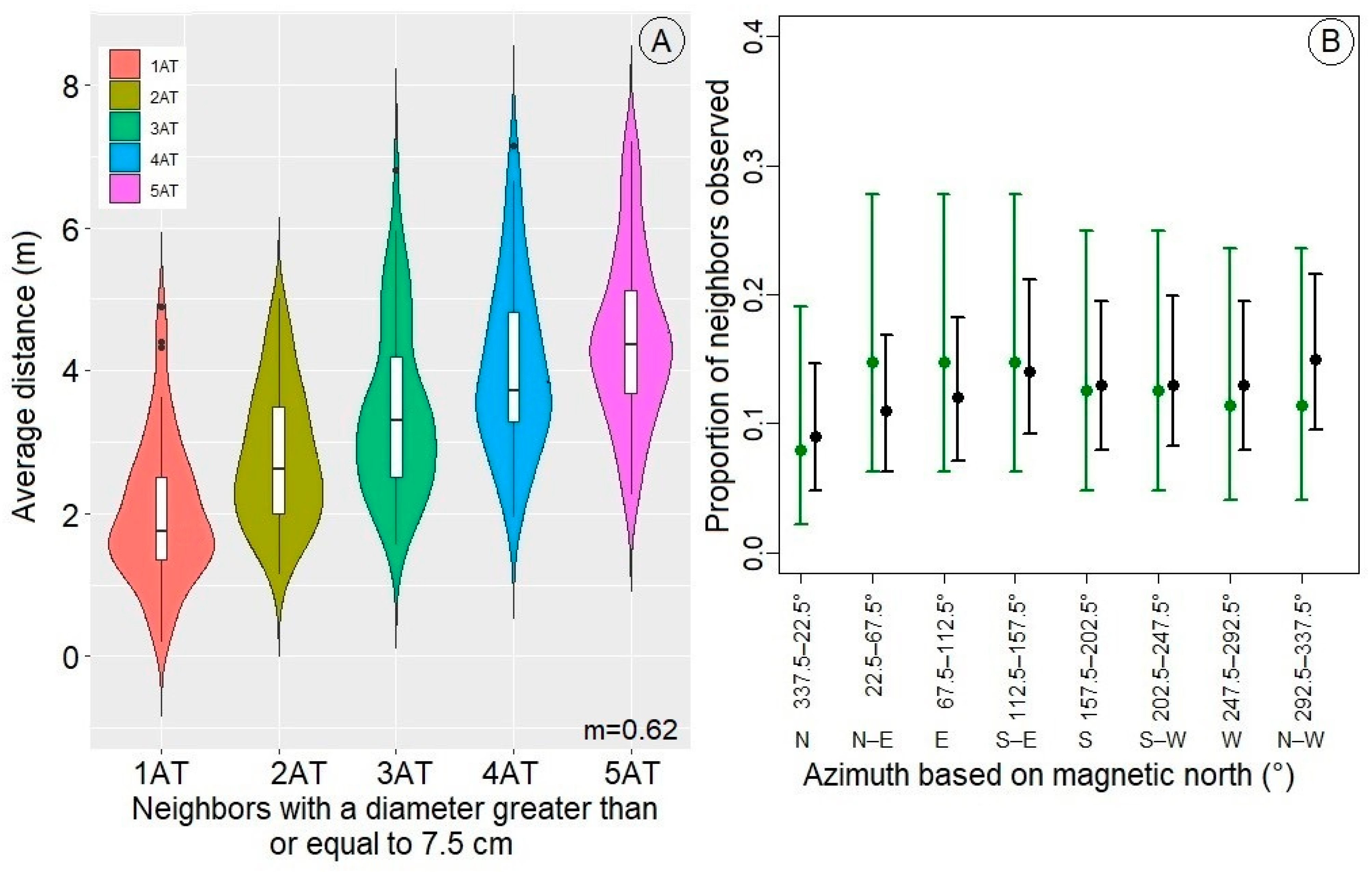
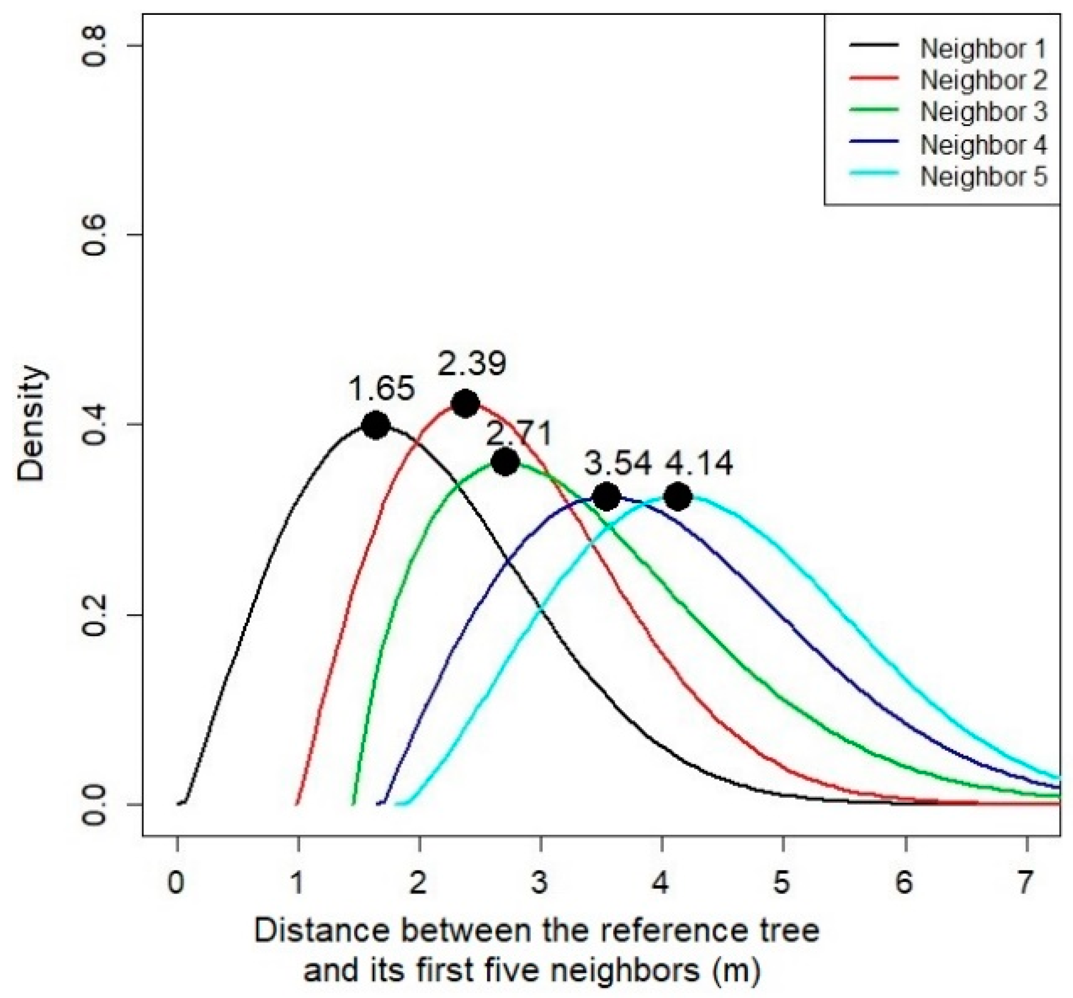
3.1. Distribution of the Neighbors and the Effect of Distance from the Neighbors

When the neighbors were arranged in order from closest to farthest, it was observed that the neighbors occupying the first position, starting from the center outward, had a mean distance of 2 m. The subsequent neighbors were located at mean distances of 2.8, 3.4, 4.1, and 4.5 m, resulting in a regression slope of 0.62 (Figure 2A). These neighbors had a single-mode distribution (Figure 2A). Among the observed neighbors, 33% were A. hickelii, while 67% were comprised of other species, mainly Pinus and Quercus. The distribution of the neighbors around each reference tree appeared to be relatively uniform, with no significant concentrations observed in any particular azimuth quadrant. When the RT contour was divided into eight quadrants based on the azimuth, the proportion of observed neighbors was similar across all quadrants, and no significant differences were observed (Figure 2B).

Distance was found to have a significant effect (p-value < 0.05) only when neighbor dimensions were larger than RT dimensions (

Table 2. Regression coefficients when evaluating the responses of the diameter at breast height (DBH) and the total height (TH) to the unit change in the average distance of the first five neighbors of A. hickelii. RT is the reference tree, SE is the standard deviation, the T-value is the t-score, the p-value is the value of the probability against the null hypothesis, and R² is the coefficient of determination.

Non-Standardized Coefficients Associated with the Neighbor’s Distance
Variable Assessed	Grouping Criteria	Coefficients	SE	T-Value	p-Value	R2
DBH	Ungrouped	−4.82	6.95	−0.694	0.492	0.011
DBH	DBH of the RT > any of the neighbors	−5.460	8.758	−0.623	0.547	0.037
DBH	DBH of the RT is < any of its neighbors	1.132	0.464	2.441	0.031	0.332
TH	Ungrouped	−3.394	3.838	−0.884	0.381	0.018
TH	TH of the RT > any of the neighbors	0.357	6.963	0.051	0.960	0.0003
TH	TH of the RT is < any of its neighbors	−1.218	0.386	−3.153	0.020	0.624
Standardized coefficients associated with the neighbor’s distance
DBH	Ungrouped	−0.200	0.288	−0.694	0.492	0.011
DBH	DBH of the RT > any of the neighbors	−0.227	0.364	−0.623	0.547	0.037
DBH	DBH of the RT is < any of its neighbors	0.047	0.019	2.441	0.033	0.332
TH	Ungrouped	−0.254	0.287	−0.884	0.381	0.018
TH	TH of the RT > any of the neighbors	0.026	0.513	0.051	0.960	0.0003
TH	TH of the RT is < any of its neighbors	−0.090	0.028	−3.153	0.020	0.624

), but when neighbors possessed smaller dimensions, the effect of distance was not significant, as the probability values against the null hypothesis were greater than 0.5 (Table 2). When neighbors were larger, the rate of change suggested that, for every meter that the neighbor distance increased, there was an average gain of 1.132 (±0.464) cm in the normal diameter of the RT. In contrast, height appears to respond inversely, as for every meter that neighbor distance increases, a coefficient equal to −1.218 m was observed; that is, height growth appears to be inhibited as the neighbor distance increases. When examining the unit impact of the mean neighbor distance, the standardized coefficients revealed that the neighbor distance has a two times greater impact on the TH than on the DBH of the RTs (Table 2). Distance manages to explain 62.4% of the total variability in height and 33.2% of the total variability in DBH (Table 2).

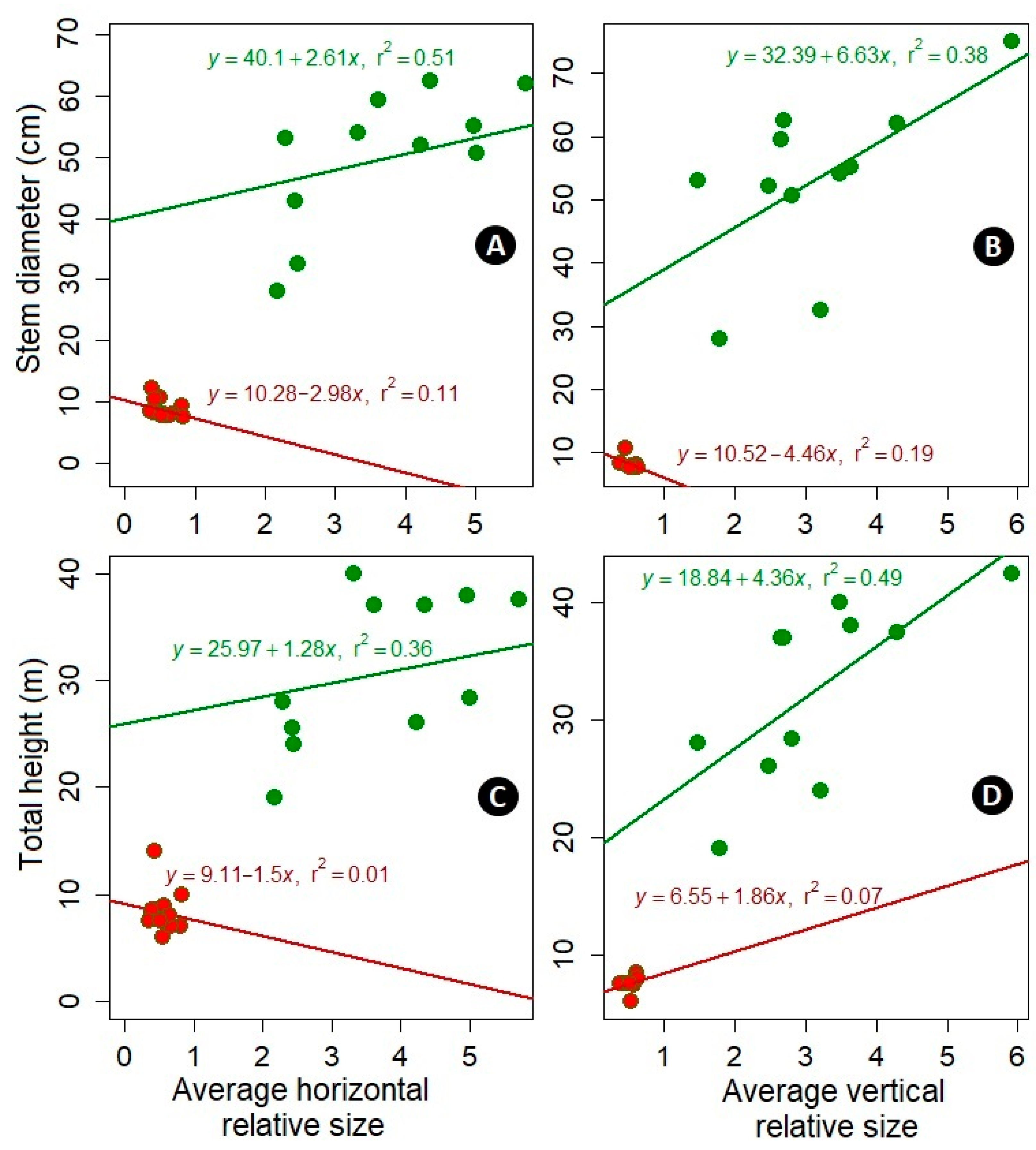
3.2. Effect of Neighbors Due to Their Sizes

A high and significant correspondence was observed between the dependent variables and the relative size, both vertical and horizontal. For example, when considering the standardized coefficients, the horizontal relative size had a 1.08 times greater impact on the DBH than on the height, without pooling the data (

Table 3. Regression coefficients when testing the hypothesis of null incidence of horizontal and vertical relative sizes in the unit change in the diameter at breast height (DBH) and the total height (TH) of A. hickelii. RT is the reference tree, SE is the standard deviation, the T-value is the t-score, the p-value is the value of the probability against the null hypothesis, and R² is the coefficient of determination.

Variable Assessed	Grouping Criteria	Coefficients	SE	T-Value	p-Value	R2
Non-standardized coefficients associated with the horizontal relative size
DBH	Ungrouped	5.909	0.648	8.906	<0.001	0.648
DBH	DBH of the RT > any of the neighbors	2.611	0.808	3.233	0.009	0.511
DBH	DBH of the RT is < any of its neighbors	−2.980	2.489	−1.197	0.254	0.107
TH	Ungrouped	3.140	0.394	7.973	<0.001	0.596
TH	DBH of the RT > any of the neighbors	1.275	0.540	2.360	0.040	0.358
TH	DBH of the RT is < any of its neighbors	−1.497	3.503	−0.427	0.676	0.015
Non-standardized coefficients associated with the vertical relative size
DBH	Ungrouped	14.131	1.074	13.157	<0.001	0.801
DBH	TH of the RT > any of the neighbors	6.626	2.844	2.330	0.045	0.376
DBH	TH of the RT is < any of its neighbors	−4.465	3.751	−1.190	0.279	0.191
TH	TH ungrouped	8.002	0.539	14.836	<0.001	0.837
TH	TH of the RT > any of the neighbors	4.362	1.490	2.928	0.017	0.488
TH	TH of the RT < any of the neighbors	1.859	2.816	0.660	0.534	0.068
Standardized coefficients associated with the horizontal relative size
DBH	Ungrouped	0.805	0.090	8.906	<0.001	0.648
DBH	DBH of the RT > any of the neighbors	0.356	0.110	3.233	0.009	0.511
DBH	DBH of the RT is < any of its neighbors	−0.406	0.339	−1.197	0.254	0.107
TH	Ungrouped	0.773	0.097	7.973	<0.001	0.596
TH	DBH of the RT > any of the neighbors	0.313	0.133	2.360	0.039	0.358
TH	DBH of the RT is < any of its neighbors	−0.368	0.862	−0.427	0.677	0.015
Standardized coefficients associated with the vertical relative size
DBH	Ungrouped	0.895	0.068	13.160	<0.001	0.801
DBH	TH of the RT > any of the neighbors	6.626	2.844	2.330	0.044	0.376
DBH	TH of the RT is < any of its neighbors	−4.465	3.751	−1.190	0.278	0.191
TH	TH ungrouped	0.915	0.062	14.840	<0.001	0.837
TH	TH of the RT > any of the neighbors	4.362	1.490	2.928	0.017	0.488
TH	TH of the RT < any of the neighbors	1.859	2.816	0.660	0.534	0.067

). This predictor explained 64.8% of the variability in the first variable and 59.6% of the variability in the second variable. On the other hand, the vertical relative size exhibited similar influences on both response variables, with standardized coefficients of 0.915 for height and 0.895 for diameter (Table 3).

Close examination revealed that, when the reference trees had their five smallest neighbors, for every cm increase in the horizontal relative (ratio), there was a mean gain of 2.61 cm in the DBH and a 1.28 m mean gain in the total height of A. hickelii trees (Table 3, Figure 3A,C). For every cm increase in the vertical relative proportion, there was a mean gain in diameter of 6.63 cm and a 4.36 m gain in the total height (Table 3, Figure 3B,D). When the RT had its five largest neighbors, the rates of change in the response variables were negative in most cases (Table 3, Figure 3A–C), suggesting inhibition of the diameter and height growth.

In general, when the first five neighboring trees were larger than the RT, negative regression coefficients were observed in the majority of cases, indicating growth inhibition. Nonetheless, it is worth noting that not all of these coefficients reached statistical significance (Table 3).

3.3. Neighbor Effect Due to Size, Distance, and Species

Taking into account the standardized coefficients and the percentages of variability in the regression model, as previously observed, distance has a greater impact on the TH than on the DBH. However, when considering the combined effect of distance and neighbor size, the regression coefficients undergo changes. For instance, the joint effect of the relative horizontal distance and the mean distance of the first five neighbors was significant for predicting both the DBH and the total height of the reference trees. Together, these variables explained 18.11% of the total variability in the DBH and 13.83% of the total variability in the total height (Table S1). On the other hand, the vertical relative proportion combined with distance accounted for 9.69% of the total variability in the DBH and 7.19% of the variability in the total height (Table S1).

Cohen’s index, which measures the relative strength of the differences between the means of the variables of interest attributed to the species of the neighbors, revealed that the effect size is greater when the neighbors belong to the same species compared to when they belong to different species. This was particularly evident for the first, second, fourth, and fifth neighbors (Table S2). For instance, when examining the DBH response in relation to the neighbors occupying the first position (1AT), a Cohen’s index of 0.44 was observed. This indicates that the average diameter of the reference trees was 0.44 standard deviations larger when their competitors were of the same species compared to when they were of different species. In contrast, the height variable exhibited an index equal to 0.58, implying that the heights were 0.58 standard deviations greater when the neighbors were of the same species rather than different species (Table S2). The highest Cohen’s index was observed for DBH when evaluating the effect of neighbors occupying the fifth position, while the smallest index was observed for the TH variable when evaluating the effect of neighbors in the third position (Table S2).

4. Discussion

4.1. Evidence of Asymmetric Competition

It has been documented that competition among plants at the individual scale can be symmetrical or asymmetrical [9,25]. In the first case, it implies that the effects of competition between larger and smaller individuals are similar, which is also known as resource depletion competition [25]. Asymmetric competition, on the other hand, occurs when larger individuals disproportionately take the available resources, suppressing the growth and development of smaller individuals [25,26,27].

The results of this study suggest that the distance of neighbors has a significant effect (p-value < 0.05) on RTs only when the dimensions of those neighbors are larger than those of the reference trees (Table 2 and Table 3). Even so, when neighbors have smaller dimensions, the effect of distance is not significant. In the latter case, the probability values against the null hypothesis were greater than 0.05 (Table 3). This result suggests that competition in the studied population is asymmetric, meaning that the intensity of the neighbor incidence is proportional to the discrepancy in size between A. hickelii and its closest competitors: the greater the discrepancy, the greater the impact.

Understanding how the individuals of interest respond to variations in size and distance from neighboring trees will provide insight into potential threats to their survival. Specific actions, such as selective thinning, controlling the distance from neighboring trees, or implementing strategies to create a more favorable environment for the species’ survival, can be taken.

The distance variable directly measures the spacing between individuals, eliminating the need for quadrants and thus removing the effect of the quadrat size [8]. In this study, three groups of neighbors could be classified based on species: those with homospecific neighbors, those with heterospecific neighbors, and those with mixed neighbors (Figures S1 and S2). According to empirical observations, the mean distances of the first five neighbors were, on average, 2, 2.8, 3.4, 4.1, and 4.5 m (Figure 2A). An important observation is that, despite being a shade-tolerant species [1], the total height of A. hickelii is more sensitive to the average variation in distance from its neighbors compared to the DBH (Table 2). This suggests that the proximity and arrangement of neighboring trees have greater impacts on the height growth of A. hickelii than on the trunk diameter. The height of a tree is crucial for light capture and therefore plays an important role in competitive interactions.

On the other hand, a complementary analysis using the Weibull function revealed that the mean distance of the first five neighbors has an asymmetric distribution with a rightward tail, although the farthest neighbors tend to have a symmetric distribution (Figure 4). According to this model, the distance at which the probability of finding the first neighbor of A. hickelii is maximized, regardless of the species, and in situations where that neighbor has a DBH of equal to or greater than 7.5, it is at a distance of 1.65 m.

4.2. Vertical Relative Size Has a Greater Effect Than the Horizontal Relative Size

Quantifying the responses of the A. hickelii tree diameter and height to a unit change in the relative sizes of their neighbors is important for effectively understanding plant interactions in their natural environment [11]. The results reveal that the competitors of the studied species have a stronger impact when their dimensions exceed those of the target trees. In such cases, for every meter increase in distance from the neighbor, there is an average gain of 1.132 cm in the normal diameter of the RT (Table 2). On the other hand, height appears to respond relatively more strongly but inversely, as a change rate of −1.218 m was observed for every meter increase in the neighbor distance (Table 2). This result is logical because as the density decreases, trees exert less effort to attain greater heights. Conversely, at higher densities, trees strive to grow vertically in order to outcompete their competitors [28,29].

In general, the DBH exhibited a response that was 1.04 times greater than that of the total height in relation to the variation of the horizontal relative size. This predictor was able to explain 64.8% of the variability in the first variable and 59.6% of the variability in the second variable (Table 3). On the other hand, the vertical relative size had a relatively higher standardized coefficient for height (0.915) compared to the DBH (0.895). It was observed that when the reference trees had their five smallest neighbors (i.e., none of the five neighbors was larger than the RT), each cm increase in the horizontal relative resulted in a mean gain of 2.61 cm in the normal diameter and a mean gain of 1.28 m in the total height (Table 3, Figure 3A). Similarly, for each cm increase in the vertical relative proportion, a mean gain of 6.63 cm in diameter and a mean gain of 4.36 m in total height were observed (Table 3). So, it was confirmed that the effect size of the vertical relative proportion is greater than that of the horizontal relative proportion.

Considering the standardized coefficients (Table 3), the relative vertical size was consistently larger than the relative horizontal size in most cases. This implies that the height has a more significant impact on the population of A. hickelii compared to the discrepancy in the DBH. This finding is in partial agreement with Duchesneau et al.’s [30] observations for balsam fir. The dominance of vertical size in influencing population dynamics could be attributed to the competition for space and access to light, particularly during early growth stages [31,32]. In the sampling area, the highest concentration of A. hickelii individuals was on steep slopes facing north and northeast, where competition for light is likely more intense (sunlight is slanting in places with northern exposure). As the species advances through the growth stages, access to sunlight becomes increasingly vital for photosynthesis, and taller trees might have a competitive advantage in terms of obtaining this resource. Still, the effect of the DBH discrepancy should not be overlooked, as it also plays a vital role in competition. Trees with larger DBH dimensions possess larger root systems [33], enabling them to access and utilize more underground resources such as water and nutrients [34].

4.3. The Roles of Species, Distance, and Size

The distance and size of neighboring trees can significantly influence various ecological processes and the growth of the species of interest. For instance, there is competition for available resources such as sunlight, water, and nutrients [35,36,37]. This study suggests that the size of the neighbors has a significant effect on A. hickelii individuals, only when the neighbors are larger than the reference trees. This could be due to larger trees capturing more sunlight and extracting greater amounts of water and nutrients from the soil, reducing the resources available to smaller neighboring trees. In this context, some plants prioritize height growth at the expense of lateral growth [38,39], which might be occurring in the studied population.

Another noteworthy factor is that the size of the effect is larger when the neighbor is of the same species compared to the effect of a neighbor from another species. The intraspecific competition has more significant impacts on the growth and development of A. hickelii than interspecific competition (Table S2). This is reasonable considering the species’ restricted geographic distribution, which is confined to small patches. As a result, individuals of A. hickelii would compete for the same limited resources and have similar resource requirements.

On the other hand, microtopography plays a vital role in the study of the distribution of plants that exhibit non-uniform and discontinuous patterns [21,40], such as A. hickelii. Future research will focus on analyzing the local topography, which is characterized by fluctuations in exposure, concavity, and slope over a few kilometers. It will also be investigated as to whether topographic features influence the frequency distribution of natural regeneration, which will be mature trees in the coming decades. Additionally, the application of alternative methods to explain the rates of change in those sectors of the conditional distribution that are far from the average [41] as well as the calculation of conventional competition indices based on the stem diameter and distance [42,43] are also being considered for further research.

5. Conclusions

Gaining a comprehensive understanding of competitive dynamics and the factors impacting the growth of Abies hickelii is important for efficient management and conservation endeavors. We conclude that the studied species experiences asymmetric competition with its first five neighbors. The height of the species under study demonstrates higher sensitivity to the average variation in the neighbor distance as compared to the diameter at breast height. Additionally, the impact of competition is more noticeable when the neighboring tree is of the same species than when it belongs to a different species. Taking these results into account, as a preliminary recommendation, selective thinning could be implemented during the early stages of growth to promote diameter and root system development. While no optimum distance between individuals has been investigated here, decision-makers could gradually increase the spacing between trees as they attain larger dimensions. Given the presence of significant intraspecific competition, priority for removal should be given to individuals of the same species. Transplanting these removed individuals to neighboring areas within the species’ range could be a viable conservation strategy. These practices would facilitate the expansion of healthier trees with adequate access to light, nutrients, and underground resources, thereby contributing to the long-term sustainability of the species.

References

1. Rehder, A. The firs of Mexico and Guatemala. J. Arnold Arbor. 1939, 20, 281–287. Available online: https://www.biodiversitylibrary.org/partpdf/21103 (accessed on 25 May 2023). [CrossRef]
2. IUCN. The International Union for Conservation of Nature’s Red List of Threatened Species. 2023. Available online: https://www.iucnredlist.org/en (accessed on 27 June 2023).
3. Farjon, A. Abies hickelii. The IUCN Red List of Threatened Species 2013, e.T42286A2969866. 2013. Available online: https://www.iucnredlist.org/species/42286/2969866 (accessed on 26 May 2023).
4. Charlesworth, D.; Willis, J.H. The genetics of inbreeding depression. Nat. Rev. Genet. 2009, 10, 783–796. [Google Scholar] [CrossRef] [PubMed]
5. Gong, W.; Gu, L.; Zhang, D. Low genetic diversity and high genetic divergence caused by inbreeding and geographical isolation in the populations of endangered species Loropetalum subcordatum (Hamamelidaceae) endemic to China. Conserv. Genet. 2010, 11, 2281–2288. [Google Scholar] [CrossRef]
6. Bello, C.H.Á.; Mata, L.L. Distribución y análisis estructural de Abies hickelii (flous & gaussen) en México. Interciencia 2001, 26, 244–251. [Google Scholar]
7. Cogoni, D.; Sulis, E.; Bacchetta, G.; Fenu, G. The unpredictable fate of the single population of a threatened narrow endemic Mediterranean plant. Biodivers. Conserv. 2019, 28, 1799–1813. [Google Scholar] [CrossRef]
8. Clark, P.J.; Evans, F.C. Distance to nearest neighbor as a measure of spatial relationships in populations. Ecology 1954, 35, 445–453. [Google Scholar] [CrossRef]
9. Weiner, J. Neighbourhood interference amongst Pinus rigida individuals. J. Ecol. 1984, 72, 183–195. [Google Scholar] [CrossRef]
10. Goldberg, D.E. Neighborhood competition in an old-field plant community. Ecology 1987, 68, 1211–1223. [Google Scholar] [CrossRef]
11. Stoll, P.; Weiner, J. A Neighborhood View of Interactions among Individual Plants. 2000. Available online: https://edoc.unibas.ch/15365/1/20180110105505_5a55e2f91b17e.pdf (accessed on 27 June 2023).
12. Balandier, P.; Collet, C.; Miller, J.H.; Reynolds, P.E.; Zedaker, S.M. Designing forest vegetation management strategies based on the mechanisms and dynamics of crop tree competition by neighbouring vegetation. Forestry 2006, 79, 3–27. [Google Scholar] [CrossRef]
13. Mack, R.N.; Harper, J.L. Interference in dune annuals: Spatial pattern and neighbourhood effects. J. Ecol. 1977, 65, 345–363. [Google Scholar] [CrossRef]
14. Biging, G.S.; Dobbertin, M.A. comparison of distance-dependent competition measures for height and basal area growth of individual conifer trees. For. Sci. 1992, 38, 695–720. [Google Scholar]
15. Prodan, M. Punktstichprobe fur die forsteinrichtung [Point sampling for forest inventory]. Forst. Holzwirt. 1968, 23, 225–226. [Google Scholar]
16. Ammann, P.; Waldbau, F. Erfolg der Jungwaldpflege im Schweizer Mittelland? Analyse und Folgerungen (Essay) [Is young growth tending successful in the Swiss plateau region? Analysis and implications (essay)]. Schweiz Z Forstwes 1969, 164, 262–270. Available online: https://ethz.ch/content/dam/ethz/special-interest/usys/ites/waldmgmt-waldbau-dam/documents/unterrichtshilfen/Management/Jungwaldpflege-Ammann-3013 (accessed on 25 July 2023). [CrossRef]
17. Lynch, T.B.; Rusydi, R. Distance sampling for forest inventory in Indonesian teak plantations. For. Ecol. Manag. 1999, 113, 215–221. [Google Scholar] [CrossRef]
18. Caeiro, F.; Mateus, A. Package ‘Randtests’. 2022. Available online: https://cran.r-project.org/web/packages/randtests/randtests.pdf (accessed on 27 June 2023).
19. Mangiafico, S.S. An R Companion for the Handbook of Biological Statistics. 2015. Available online: https://rcompanion.org/documents/RCompanionBioStatistics.pdf (accessed on 27 April 2023).
20. Clopper, C.; Pearson, E.S. “The use of confidence or fiducial limits illustrated in the case of the binomial”. Biometrika 1934, 26, 404–413. [Google Scholar] [CrossRef]
21. Antúnez, P.; López Serrano, P.M.; González Adame, G.; Rubio Camacho, E.A.; Mendoza Díaz, M.M. Efecto de la altitud, pendiente y exposición geográfica en la distribución de helechos arborescentes. Acta Bot. Mex. 2022, 29, e1962. [Google Scholar] [CrossRef]
22. Torchiano, M.; Torchiano, M.M. Package “Effsize”. 2020. Available online: https://cran.r-project.org/web/packages/effsize/effsize.pdf (accessed on 10 June 2023).
23. Robinson, A.P.; Hamann, J.D. Forest Analytics with R: An Introduction; Springer Science & Business Media: New York, NY, USA, 2010. [Google Scholar]
24. Prodan, M.; Peters, R.; Cox, F.; Real, P. Mensura Forestal; Agroamerica: San José, Costa Rica, 1997. [Google Scholar]
25. Weiner, J. Asymmetric competition in plant populations. Trends Ecol. Evol. 1990, 5, 360–364. [Google Scholar] [CrossRef] [PubMed]
26. Connolly, J.; Wayne, P. Asymmetric Competition between Plant Species. Oecologia 1996, 108, 311–320. [Google Scholar] [CrossRef] [PubMed]
27. Freckleton, R.P.; Watkinson, A.R. Asymmetric competition between plant species. Funct. Ecol. 2001, 15, 615–623. [Google Scholar] [CrossRef]
28. Drew, T.J.; Flewelling, J.W. Some recent Japanese theories of yield-density relationships and their application to Monterey pine plantations. For. Sci. 1977, 23, 517–534. [Google Scholar] [CrossRef]
29. Trouvé, R.; Bontemps, J.D.; Seynave, I.; Collet, C.; Lebourgeois, F. Stand density, tree social status and water stress influence allocation in height and diameter growth of Quercus petraea (Liebl.). Tree Physiol. 2015, 35, 1035–1046. [Google Scholar] [CrossRef] [PubMed]
30. Duchesneau, R.; Lesage, I.; Messier, C.; Morin, H. Effects of light and intraspecific competition on growth and crown morphology of two size classes of understory balsam fir saplings. For. Ecol. Manag. 2001, 140, 215–225. [Google Scholar] [CrossRef]
31. Pollastrini, M.; Holland, V.; Brüggemann, W.; Koricheva, J.; Jussila, I.; Scherer-Lorenzen, M.; Berger, S.; Bussotti, F. Interactions and competition processes among tree species in young experimental mixed forests, assessed with chlorophyll fluorescence and leaf morphology. Plant Biol. 2014, 16, 323–331. [Google Scholar] [CrossRef]
32. Sevik, H.; Cetin, M.; Kapucu, O. Effect of light on young structures of Turkish fir (Abies nordmanniana subsp. bornmulleriana). Oxid. Commun. 2016, 39, 485–492. [Google Scholar]
33. Drexhage, M.; Colin, F. Estimating root system biomass from breast-height diameters. Forestry 2001, 74, 491–497. [Google Scholar] [CrossRef]
34. Zanetti, C.; Vennetier, M.; Mériaux, P.; Provansal, M. Plasticity of tree root system structure in contrasting soil materials and environmental conditions. Plant Soil 2015, 387, 21–35. [Google Scholar] [CrossRef]
35. Casper, B.B.; Jackson, R.B. Plant competition underground. Ann. Rev. Ecol. Syst. 1997, 28, 545–570. [Google Scholar] [CrossRef]
36. Contreras, M.A.; Affleck, D.; Chung, W. Evaluating tree competition indices as predictors of basal area increment in western Montana forests. For. Ecol. Manag. 2011, 262, 1939–1949. [Google Scholar] [CrossRef]
37. Forrester, D.I.; Kohnle, U.; Albrecht, A.T.; Bauhus, J. Complementarity in mixed-species stands of Abies alba and Picea abies varies with climate, site quality and stand density. For. Ecol. Manag. 2013, 304, 233–242. [Google Scholar] [CrossRef]
38. Schmitt, J. Reaction norms of morphological and life-history traits to light availability in Impatiens capensis. Evolution 1993, 47, 1654–1668. [Google Scholar] [CrossRef]
39. Schmitt, J.; Wulff, R.D. Light spectral quality, phytochrome and plant competition. Trends Ecol. Evol. 1993, 8, 47–51. [Google Scholar] [CrossRef] [PubMed]
40. Antúnez, P. Influence of physiography, soil and climate on Taxus globosa. Nord. J. Bot. 2021, 39. [Google Scholar] [CrossRef]
41. Antúnez, P.; Wehenkel, C.; Hernández-Díaz, J.C.; Garza-López, M. Quantile regression as a complementary tool for modelling biological data with high variability. J. Trop. For. Sci. 2023, 35, 130–140. Available online: https://www.jstor.org/stable/48723350 (accessed on 7 August 2023). [CrossRef]
42. Martin, G.L.; Ek, A.R. A comparison of competition measures and growth models for predicting plantation red pine diameter and height growth. For. Sci. 1984, 30, 731–743. [Google Scholar] [CrossRef]
43. Johann, K. Der A-Wert, ein objektiver Parameter zur Bestimmung der Freistellungsstärke von Zentralbäumen. In Tagungsbericht, Deutscher Verband Forstlicher Versuchsanstalten—Sektion Ertragskunde; [The A-value, an objective criterion for estimating the release of central trees from competition]; DVFFVA: Weibersbrunn, Germany, 1982; pp. 146–158. [Google Scholar]
Figure 1. Location of the Abies hickelii population in Xagacía, Oaxaca, Mexico.
Forests 14 01654 g001
Figure 2. The interquartile range of the five nearest neighbors is depicted in the violin diagram (A) as well as a graphical representation of the proportion of neighbors with their 95% confidence intervals (B). The positions occupied by the neighbors are denoted as 1AT, 2AT, 3AT, 4AT, and 5AT, indicating the first, second, third, fourth, and fifth positions, respectively; m is the slope given by the linear regression. The green lines in panel (B) represent the confidence intervals for the proportions of neighbors belonging to the species A. hickelii, while the black lines represent neighbors belonging to other species. The cardinal directions are abbreviated as follows: N: north, NE: northeast, E: east, SE: southeast, S: south, SW: southwest, W: west, and NW: northwest.
Forests 14 01654 g002
Figure 3. Scatter plots showing the relationship between the horizontal relative size and the DBH (A), the vertical relative size and the DBH (B), the horizontal relative size and the total height (C), and the vertical relative size and the total height (D). The data are color-coded in green when the DBH of the RT > any of the neighbors, while they are marked in red when the DBH of the RT is < any of its neighbors. In panels (C,D), the green color denotes that the TH of the RT is > any of the neighbors and the red color denotes that the TH of the RT < any of the neighbors.
Forests 14 01654 g003
Figure 4. Distance distribution of the first five neighbors of Abies hickelii, according to the three-parameter Weibull function. The peak value of each density curve represents the distance at which the probability of encountering a neighbor is maximized, according to the three-parameter Weibull density function.
Forests 14 01654 g004