

A Review on Acoustics of Wood as a Tool for Quality Assessment
School of Science, RMIT University, 124 La Trobe Street, Melbourne 3001, Australia
Forests 2023, 14(8), 1545; https://doi.org/10.3390/f14081545
Submission received: 3 April 2023
/
Revised: 7 July 2023
/
Accepted: 7 July 2023
/
Published: 28 July 2023
(This article belongs to the Special Issue Reviews on Structure and Physical and Mechanical Properties of Wood)
Abstract
:Acoustics is a field with significant application in wood science and technology for the classification and grading, through non-destructive tests, of a large variety of products from standing trees to building structural elements and musical instruments. In this review article the following aspects are treated: (1) The theoretical background related to acoustical characterization of wood as an orthotropic material. We refer to the wave propagation in anisotropic media, to the wood anatomic structure and propagation phenomena, to the velocity of ultrasonic waves and the elastic constants of an orthotropic solid. The acoustic methods for the determination of the elastic constants of wood range from the low frequency domain to the ultrasonic domain using direct contact techniques or ultrasonic spectroscopy. (2) The acoustic and ultrasonic methods for quality assessment of trees, logs, lumber and structural timber products. Scattering-based techniques and ultrasonic tomography are used for quality assessment of standing trees and green logs. The methods are based on scanning stress waves using dry-point-contact ultrasound or air-coupled ultrasound and are discussed for quality assessment of structural composite timber products and for delamination detection in wood-based composite boards. (3) The high-power ultrasound as a field with important potential for industrial applications such as wood drying and other applications. (4) The methods for the characterization of acoustical properties of the wood species used for musical instrument manufacturing, wood anisotropy, the quality of wood for musical instruments and the factors of influence related to the environmental conditions, the natural aging of wood and the effects of long-term loading by static or dynamic regimes on wood properties. Today, the acoustics of wood is a branch of wood science with huge applications in industry.
Keywords:
acoustics; solid wood; elastic constants; ultrasound; wood products; trees; logs; lumber; LVL; glulam1. Introduction
Acoustics is a field with significant application in wood science and technology for the classification and grading of a large variety of products, from standing trees to building structural elements and musical instruments, using non-destructive tests [1,2,3]. The acoustics of wood employs mechanical waves which are sensitive to key parameters of this material, such as the density, the grain angle, the annual ring curvature, the elastic moduli, the moisture content, the degradation by pathogenic factors, etc. The experimental data collected with different acoustic methods are difficult to interpret correctly because of numerous factors acting on the phenomena related to the propagation of acoustic waves in solid wood or wood-based composites. Therefore, there is a need to have a good understanding of phenomena related to the wave propagation in media of various complexity, such as the orthotropic media which are described in the section: Theoretical Aspects Related to Acoustical Characterization of Wood. The following sections discuss acoustic and ultrasonic methods for quality assessment of trees, logs, lumber and structural timber products. Special attention is given to methods for the characterization of acoustical properties of wood species used for musical instrument manufacturing. High power ultrasound is a field with important potential for industrial applications to wood drying, among others.
2. Theoretical Aspects Related to the Acoustical Characterization of Wood
In this section, our discussion is focused on theoretical aspects related to the characterization of the mechanical constants of wood. Currently, the engineering constants which characterize solids are Young’s modulus E, the shear modulus G and the Poisson coefficient ν. The number of these engineering constants for solids depends on their nature, which could be isotropic or anisotropic. In what follows, we will discuss the elastic symmetry of various media and the acoustical method for their characterization.
2.1. Elastic Symmetry of Propagation Media
Elastic waves can propagate in solid media of various symmetries and structural complexity. The simplest case of elastic symmetry is that of an isotropic solid. For solid wood and for wood-based composites, orthotropic and transverse isotropic symmetries are most frequently observed. For simplicity, we will start by analyzing an isotropic solid. The solids are assumed to be homogeneous.
2.1.1. Isotropic Solid
The simplest elastic symmetry is that of an isotropic solid, with only three independent constants, E, G and the Poisson ratio ν. The relationships between those constants are shown as follows: , where E is Young’s modulus (which is the ratio of longitudinal stress to longitudinal strain in the same direction of a rod), G is the shear modulus (which is the ratio of the deviatoric stress to the deviatoric strain), ν is the Poisson’s ratio (the ratio of the transverse contraction of a sample to its longitudinal extension, under tensile stress).
The velocity of propagation of a compressional longitudinal wave V in an infinite isotropic solid, of density ρ and initially assumed to be stress-free, is related to the elastic constant E by Vlongitudinal wave = .
The velocity of propagation of a shear wave V in an infinite isotropic solid, of density ρ and initially assumed to be stress-free, is related to the elastic constant G, or the shear modulus, by Vshear wave = .
2.1.2. Anisotropic Solids
The elastic properties of anisotropic solids can be defined by the generalized Hooke’s law relating the volume average of stress [σij] to the volume average of strain [εkl] by the elastic constants [Cijkl] in the form
or
where [Cijkl] are termed elastic stiffnesses and [Sijkl] the elastic compliances, and the indices i, j, k, l correspond to 1, 2, 3, 4.
[σij] = [Cijkl] [εkl]
[εkl] = [Sijkl] [σij]
Stiffnesses and compliances are fourth-rank tensors. In his book, Hearmon [4] noted that “the use of the symbols for compliances [S] and [C] for stiffness is now almost invariably followed.” This is the notation that will be used hereafter. [Cijkl] could be written, following the general convention on matrix notation, as [Cij], in terms of two-suffix stiffnesses, or symbolically as [C]. Similarly, [Sijkl] could be written as [Sij] or [S]. Stiffnesses and compliances are fourth-rank tensors.
In many applications it is much simpler to write Equations (1) and (2) in the following condensed form: [C] = [S]−1 and [S] = [C]−1. The engineering constants—Young’s moduli, shear moduli and Poisson ratios—are terms of a compliance matrix. A complete set of elastic constants of wood are given in [5].
Experimentally, the terms of the [C] matrix could be determined from ultrasonic measurements, whereas those of the [S] matrix could be determined from static tests. However, the engineering constants, namely Young’s moduli E, shear moduli G and Poisson ratios can be determined by resonance frequency methods.
From Equation (1) it can be deduced that since strain is dimensionless the stiffnesses have the same dimensions as the stresses [the units used presently are Newtons per square meter (N/m2) or megapascals (MPa)]. As an example, let us take the case of spruce, for which C11 = 150 × 108 N/m2 = 15,000 MPa = 15 GPa.
For solids of different symmetries such as transverse isotropic, orthotropic, etc., the stiffness matrix can be turned into a compliance matrix, following a specific procedure [6,7,8].
The origin of anisotropy, perceived as the variation in material response with direction of the applied stress, lies in the preferred organization of the internal structure of the material. The structure might be, for example, the atomic array in monocrystals; the morphological texture in polycrystalline aggregates such as metals, rocks, sand, etc.; the orientation of fibers in composites, in wood and in human tissue; or the orientation of layers in laminated plastics, plywood, etc. One instance of complex elastic symmetry is that of an orthotropic solid, because constants are influenced by three mutually perpendicular planes of elastic symmetry. For example, in the case of wood (Table 1), we have three symmetry axes related to the natural directions of growth of a tree, which are L axial or longitudinal and radial and tangential R and T with respect to the annual rings. Compressional waves can propagate in direction L, R, T and shear waves can propagate in the LR, LT and RT planes. Therefore, we can determine six elastic constants. The coupling between compressional and shear waves is given by three other corresponding terms. In a more general way, we define the axes L, R and T as axis 1, axis 2, axis 3. The corresponding stiffness matrix [C] contains nine independent constants: six diagonal terms (C11, C22, C33, C44, C55, C66) and three off-diagonal terms (C12, C13, C23).
In the case of a plywood plate, we have in total five elastic constants such as C11 and C22 = C33 and C 55 = C 66 and C12 = C13 and C23. This is the case of a solid having transverse isotropy. It can be shown that transverse isotropy is a particular case of an orthotropic solid. For isotropic materials, we have only three elastic constants: C11 = C22 = C33; C44 = C55 = C66; and C12 = C13 = C23 if we refer to the previous notation for the most complex case of an orthotropic solid. In the most general case, a material may possess only an axis of symmetry in the sense that all directions at right angles to this axis are equivalent.
The physical significance of the compliances is as follows:
- -
- S11, S22, S33 relate an extensional stress to an extensional strain, both in the same direction. For the particular symmetry of solid wood this relation gives the Young’s moduli EL, ER, and ET.
- -
- S12, S13, S23 relate an extensional strain to a perpendicular extensional stress. In this way the six Poisson’s ratios can be calculated.
- -
- S44, S55, S66 relate a shear strain to a shear stress in the same plane, and are the inverse of the terms C44, C55, C66, corresponding to planes 23, 13, 12.
Experimentally, the terms of the matrix [C] can be determined with ultrasonic methods and the terms of matrix [S] can be determined by static tests or dynamic tests in the low frequency domain. Table 2 and Table 3 give the engineering parameters of solid wood determined by static tests:
Note the large range of variation of wood density from 200 kg/m3 to 660 kg/m3. The anisotropy of wood species can be expressed by the ratio of constants as for instance EL/GRT, for balsa is 21 and for spruce is 440 and for oak is 58.5. Wood is a very anisotropic material.
Indeed, negative values of Poisson’s ratios or values greater than 1 may contradict our intuition if our main experience is in dealing with isotropic solids, but such data have been reported for composite materials [9], foam material [10], cellular materials [11], crystals [6], wood [12,13,14,15], cell walls [16] and wood-based composites [17]. Idealized two-dimensional honeycomb patterns of a transverse wood structure could produce a Poisson’s ratio ν RT in the range: −1 to +∞.
For a very wide range of European, American and tropical species, [18,19,20,21,22] deduced statistical regression models able to predict the terms of the compliance matrix as a function of density. These data may be used by modelers in finite element calculations or with non-destructively tested lumber when the elasticity moduli are required; see Table 4.
It is worth mentioning the correlation among the velocities and the engineering constants of wood as shown in Figure 1 for the resonance spruce for violins. The statistical correlations demonstrated once more that the acoustic wave propagation phenomena in wood are related to the microstructure of this material. An accurate estimation of the mechanical behavior of wood requires simultaneous views on structure and wave propagation phenomena. Wave velocities are affected by wood structure that acts as a filter. This interaction is highly revealing of the anisotropy of this material.
The highest simple correlation coefficient was between VLL and the width of the annual ring (r = −0.708). This means that high values of VLL are related to small and regular annual rings. VRR is very slightly correlated to the proportion of latewood (r = 0.210) as well as VTT, which increases slightly with the width of annual rings (r = 0.289) and with the width of latewood (r = 0.258). These correlation coefficients are not statistically significant.
Principal component analysis demonstrated that the variability of the resonance wood population studied is better explained by three variables, VLL and the Poisson ratios LT and RT. The explanation of the variability of wood density in the relatively low range of variation between 381 kg/m3 and 446 kg/m3 “is far from all the other measured physical and acoustical characteristics”. This needs some comment. The density is a scalar. The velocities are vectors, sensitive to wood structure and are able to explain better the variability of wood. Further research is needed to explain the effect of the density components and especially of the latewood density and proportion to the waves’ propagation phenomena.
However, we shall see further that in the large range of variation of the density there are significative correlations with the velocities of wood.
Another interesting aspect related to the quality of resonance wood is the low microfibril angle of about 5° [24]. This structural element contributes to the waves’ propagation in the L direction. The variation of ultrasonic velocity with microfibril angle was studied on a disk of Pinus radiata from the pith to the bark (Figure 2). In Pinus radiate, the value of the microfibril angle is between 5° and 35° and the ultrasonic velocity VLL is between 2800 m/s and 5400 m/s.
Ultrasonic velocity in the L direction was correlated with microfibril angles and the correlation coefficient is significantly high, namely −0.86. This means that high values of ultrasonic velocity correspond to low values of microfibril angles. The correlation between the modulus of rigidity (noted MOE) and the ultrasonic velocity is 0.85. No correlation was established between the microfibril angle and the air dry density of wood of Pinus radiata.
2.2. Wave Propagation in Anisotropic Media
2.2.1. Wood Structure and Propagation Phenomena
Let consider the fine structure of wood, as illustrated in Figure 3. As a first approximation wood can be considered to be made up of cellulosic tracheids or fibers oriented along the growing axis of the tree. These elements, in a simplified view are cylinders which are embedded in an amorphous lignin matrix.
From an acoustic point of view, wood structure can be considered as a rectangular system of cross ‘‘tubes’’ embedded in a matrix. It is interesting to note that in the longitudinal direction (L) the dissipation of acoustic energy takes place at the limit of the ‘‘tubes’’. Accordingly, the continuous and uniform structure of softwoods, built up by long anatomical elements, has low dissipation and provides high values for the acoustical constants. Two other aspects of microstructure could be considered: the annual ring layered structure and the difference between the R and T directions in the arrangement of cells. The fibers tend to be aligned in the R direction and randomly distributed in the T direction. This arrangement of anatomical elements could also have a significant influence on shear wave propagation and wave birefringence. The modulation of shear waves by the structure of wood must be understood in terms of both the propagation and polarization direction. The ultrasonic energy injected into a fibrous material couples into each fiber via several modes (longitudinal, transversal and circumferential). The physical properties of the cellular wall such as the density, the stiffness moduli, etc., and the shape and size of fibers or of other elements affect the transmitted ultrasonic field. Each structural element acts independently like an elementary resonator. The spatial distribution of velocities and frequencies that matched the natural fibers’ frequency could explain the acoustical behavior of wood, illustrated by its overall parameters. Wood material exhibits different length scales ranging from meters for trees and lumber and millimeters for rings as layered composites with homogeneous but anisotropic layers to micrometers for cells, rays etc., that are cellular solids with homogeneous cell walls that are fiber-reinforced laminates and to nanometers for cellulose crystals and amorphous lignin. These scales can match different acoustic wave lengths. At a 10−2 m scale, wood can be modeled as a locally orthotropic homogeneous solid. This hypothesis was used in the present discussion.
2.2.2. Type of Waves Propagation in an Anisotropic Solid
Three types of waves can propagate in solids: longitudinal waves, shear waves and surface waves (Figure 4). In longitudinal or compressional waves, particle motion in the medium is parallel to the direction of the wave front. In shear waves, particle motion is perpendicular to the wave direction. Surface waves, or Rayleigh waves, represent an oscillating motion that travels along the surface of a test piece to a depth of one wavelength. When propagated in solids depending on the specific conditions of reflection or refraction, these waves can be submitted to mode conversion. The longitudinal waves have the highest values of velocity and shear waves have the lowest velocities. Other wave modes exist such as Lamb waves or other forms of plate wave.
2.2.3. Velocity of Waves and the Elastic Constants
The propagation of waves in isotropic and anisotropic solids has been discussed in numerous reference books. Among them, I specify [6,8,26,27].
We have seen that he generalized Hook’s law can be written as
[σij] = [Cijkl] [εkl]
The strain tensor [εkl] for small deformation of the material under stress is related linearly to the displacement u as
The elastodynamic equations for a continuum with no forces acting on it are
By combining the elastodynamic equations for a continuum with no forces acting and the strain tensor [εkl] for small deformations of the material under stress related linearly to the displacement u, the equation of the wave can be written as
If we assume a plane harmonic wave with the displacement u propagating in the direction of the unit vector n, normal to the wavefront, we have
ui = Ai exp {i(kj xj − ωt)}
The unit wave vector kj can be written as
For the amplitude we can write Ai = A Pm where Pm are the components of the unit vector in the direction of displacement (polarization). After substitution, the equation of motion takes the form of Christoffel’s equations.
Christoffel’s equations supply the relations between the elastic constants Cijkl and the phase velocity vphase of ultrasonic waves propagating in the medium. These equations are valid for the most general kind of anisotropic solids.
where Cijkl = stiffness tensor; nk = direction cosines of the propagation vector; δik is the Kronecker tensor; if i = k, then δik = 1 and if i ≠ k, δik = 0; ρ = density; V—phase velocity; Pm—components of the unit vector in the direction of the displacement or polarization.
[Cijkl nj nk − δik ρ v2 phase] [Pm] = 0
By introducing the Kelvin–Christoffel tensor, Γ, we can write Γik = Cijkl nj nl
and the Christoffel equation can be written as
for which we can calculate the eigenvalues and the eigenvectors.
[Γik − δik ρ v2] [Pm] = 0
- (a)
- The Eigenvalues of Christoffel’s Equations
For an orthotropic solid, with nine terms of stiffness tensor [C] and three elastic symmetry planes we have the following relationships related to the eigenvalues of the Christoffel equation:
- -
- In symmetry plane 12: n1 = cos α; n2 = sin α; n3 = 0 and the stiffnesses C11; C22; C66; and Γ11 = C11n12 + C66n22; Γ22 = C22n22 + C66n12; Γ12 = (C12 + C66)n1n2;
- -
- In symmetry plane 13: n1 = cos α; n3 = sin α; n2 = 0 and the stiffnesses C11; C33; C55; and Γ11 = C11n12 + C55n32; Γ33 = C33n3 2 + C55n12; Γ23 = (C13 + C55)n1n3;
- -
- In symmetry plane 23: n2 = cos α; n3 = sin α; n1 = 0 and the stiffnesses C22; C33; C44; and Γ22 = C22n22 + C44n32; Γ33 = C33n32 + C44n22; Γ23 = (C23 + C44)n2n3;
The eigenvalues and the eigenvectors of Christoffel’s equations can be calculated for specific anisotropic materials. The nonzero values of the displacements—polarization—are obtained as characteristic eigenvectors corresponding with the characteristic eigenvalues which are the roots of the Christoffel equation. These solutions show that along every axis it is possible to have three types of waves, i.e., one longitudinal and two transverse.
Experimentally, by measuring the velocities, it is possible to calculate the elastic constants. Wave propagation velocities along the principal directions of elastic symmetry of an orthotropic solid are summarized in Table 4 and Table 5 for the propagation of waves in the principal directions.
If we refer to the particular case of wood, we can define the velocities as shown in Figure 5.
The velocities of longitudinal waves are VLL VRR and VTT. For these waves the direction of propagation is parallel to the direction of polarization. Shear waves have their polarization direction perpendicular to their propagation direction. For example, in the plan LR we can have VLR and VRL. Theoretically, for an orthotropic model of wood these velocities should be VLR = VRL. Experimentally, these values are always different because waves propagate in a real material having a particular structure.
The relationships among the velocities and the elastic constants for the case of the waves’ propagation out of principal directions of elastic symmetry for an orthotropic solid are given in Table 6.
It is worth mentioning that propagation out of principal directions of elastic symmetry for an orthotropic solid generates three types of waves: QL, QR and T. The energy of these waves is different. The normal wave can generate phenomena of conical refraction of waves. Ultrasonic energy propagation through wood was studied by [28,29,30,31]. In wood, as in other anisotropic materials, the group velocity vector generally differs from the phase velocity vector. The group velocity vector is normal to the slowness surface of a wave mode.
While the propagation vectors of the three modes (QL, QT and T) are identical (at the angle α), the energy flux vectors depend on the mode. The angle of energy flux deviation can be calculated and verified experimentally, by holding the sending transducer stationary while scanning with the receiving transducer for the maximum energy for each mode, keeping the transducer axes parallel. The angle of flux deviation can be calculated from the lateral beam offset and the sample thickness, using simple trigonometry [30]. The flux energy deviation angle and slowness of QL and QT waves in oak and in Douglas fir is shown in Figure 6.
The choice of these species—oak and spruce—is very illustrative because of the high anisotropy in elastic properties between the L and T directions. Wave behavior in this plane is also important in the application of ultrasonics in wood evaluation because this symmetry plane is often very accessible in practical situations. The anisotropy is more pronounced for Douglas fir than for oak and leads to a large energy flux deviation of up to 45°. The QT wave mode in oak behaves almost like an isotropic mode, its phase velocities hardly changing with propagation angle. In oak, the energy flux deviations are quite small, not exceeding 12°; however, in Douglas fir, a strong maximum in the 60° propagation direction is observed. The latewood–earlywood alternance in Douglas fir of very different densities are inhomogeneities which introduce in wave propagation a stop band effect.
Mathematical modeling as well as practical experience show that the energy flux deviation of the QT wave is particularly sensitive to the magnitude of the off-diagonal elastic constants. Acknowledging the phenomena of energy partition and energy flux deviation and adjusting the experimental design to take advantage of the additional measurable quantities will significantly improve the accuracy of ultrasonic determination of the off-diagonal elastic constants of wood.
- (b)
- The Eigenvectors of Christoffel’s Equations
From Christoffel equations, we can obtain the eigenvectors in a very simple way if two off-diagonal components of the tensor are zero. In plane 12, for an orthotropic solid, the linear equation for the displacement Pm (p1, p2, 0) associated with the quadratic factor of Equation (12) for (n1, n2, 0) is as follows:
where
If we let the polarization correspond to the same sign, i.e.,
where is the displacement angle, we obtain
and
From Equation (16), the particle displacement (polarization) is expressed in terms of phase velocity, propagation direction and stiffness constants of the solid for each plane of symmetry.
It can also be deduced that the polarization angle between the displacement vector belonging to the inner sheet of the slowness surface and the corresponding wave normal on the symmetry axis is 0°. On the axis of the solid, the wave is a pure longitudinal wave. For pure shear waves, the angle between the propagation and polarization vectors is π/2. The polarization angle changes when the propagation direction is out of the principal directions.
A better understanding of propagation phenomena in anisotropic solids is given by a tridimensional representation of slowness surfaces and corresponding displacements, as suggested by [32] with a numerical modeling method. The polarization vector is decomposed along local spherical coordinates in three components, corresponding to the longitudinal wave and to two shear waves, QT and T, or fast and slow shear waves. A holistic understanding of the acoustical properties of wood and of the anisotropy of this material is given in a three-dimensional representation. Figure 7 illustrates the characteristics of spruce and oak in a three-dimensional representation.
The slowness curves (the variation of the inverse of velocities versus the propagation direction of waves) show that the acoustical anisotropy of spruce is more pronounced than that of oak. For both species studied, the inner slowness sheets (which is the inverse of velocity VLL) exhibited a flattened ellipsoidal shape. In the planes X1-X2 or LR and X1-X3 or RT (axis X1 being the axis corresponding to the fibers’ direction) the color is more or less uniform. This means that the polarization is parallel to the propagation vector. In the plane X2-X3 the color varies from X2 to X3 and this means that the polarization varies more and more when the angle approaches the axis X3. This pattern was observed for both species. The shear waves are more sensitive to the differences between species than the longitudinal waves.
Based on previous considerations, we have seen that the three-dimensional representation of slowness surfaces in wood is related to the dynamic aspects of particle displacement of the ultrasonic wave and is associated with the wave front. This representation for wood species supplies a better understanding of ultrasonic wave propagation through this material and underlines kinematic aspects of wave propagation related to progressive mode conversion. The anisotropy of different species like spruce and oak, expressed by their acoustical behavior, is well represented in a global way. This representation is in agreement with the three-dimensional representation of other anisotropic materials [32].
2.3. Effect of Density on Ultrasonic Velocity
We have seen previously that stiffness in the L direction is calculated as CLL = V LL2 × ρ. In what follows we will analyze the variation of the velocity in the L direction with the density of the annual rings for two softwood species: jack pine and black spruce of Canadian origin (Figure 8a) [34]. Increasing density in the range from 350 kg/m3 to 510 kg/m3 causes the increase in velocity from 4000 m/s to 6000 m/s. If we refer to the density of the latewood and of the earlywood in the annual ring, we observe the same tendency of increasing of velocity with density (Figure 8b). The variation of the density in the annual ring is similar to the variation of the modulus CLL = V LL2 × ρ. (Figure 8c). Note the density of the first nine rings corresponding to juvenile wood, followed by an increasing density for the mature wood.
The presence of the reaction wood can be detected by an ultrasonic velocity method (Figure 9) [35]. In Pinus sylvestris, normal wood the velocity increased from 5500 m/s to 6000 m/s with the increasing proportion of latewood in the annual ring to a maximum of about 40% and decreases dramatically to 4000 m/s for reaction wood and juvenile wood for which the latewood is 80% from the width of the annual ring.
2.4. Effect of Moisture Content on Ultrasonic Velocity
Moisture content in wood is due to the presence of water in the wood structure under two states as free water in the lumens of cells or as bound water in the cellular wall. The fiber saturation point is at about 30%. Physical and mechanical properties of wood are affected by the moisture content, with low moisture content causing high values of the mechanical properties of wood determined with ultrasonic techniques [36]. The effect of moisture content on velocity VLL is shown in Figure 10a. Note the decreasing velocity with increasing moisture content in the range 0%–30%. After the fiber saturation point the velocity VLL is relatively unaffected by increasing the moisture content. A holistic representation of the moisture content’s simultaneous variation with the longitudinal and shear ultrasonic velocities is shown in Figure 10b and in Table 7. All values of velocities decrease with increasing moisture content.
The effect of increasing moisture content on the engineering constants are shown in Table 8, Table 9 and Table 10.
Moisture content increasing from about 10% to about 19% causes increases in all Poisson ratios. However, some of them increased spectacularly; for instance, ν LR increased by 300%, ν RL by 400% and ν RT by 160%. For Poisson ratios in the LT plane, ν:LT increased by 9.6% and ν TL increased by 7.2%. This means that the contribution of water existing mostly in the anatomic elements organized along the R direction is causing the deformation of wood. It seems that the migration of the bound water into the wood structure occurs firstly in the R direction and then in the L direction.
When comparing the values of Poisson ratios determined with ultrasonic tests and with static tests (Table 11) it can be noted that with ultrasonic tests, ν TL > 2 and ν TR > 1. The coefficients ν LR, ν LT and ν RT are in the same range. The effect of moisture content on Poisson ratios is shown in Table 12. Static measured values decrease with moisture content while values measured with an ultrasonic method increase. The ultrasonic method is more sensitive to the variation of moisture content in the anisotropic structure of wood than static tests. Table 13 gives a summary for the relationships between Poisson ratios in the same anisotropic plane.
To summarize, we can compare the effect of ultrasonic and static methods on the values of Poisson ratios as:
2.4.1. Ultrasonic Method Effect
- -
- The Poisson ratios increase with decreasing moisture content.
- -
- The planes LT and LR are mostly affected (ν ij increased with about 40%) by moisture content increasing from 9.6% to 18.7%. Water migration is firstly along the L axis and secondly along axis R.
- -
- The RT plane is affected by about 25% (the ν RT ij increased by about 22% and ν TR 30%) by moisture content increasing from 9.6% to 18.7%. Axis T is more resistant to deformation than axis R. Migration of water is along the R axis.
2.4.2. Static Compression Effect
- -
- The Poisson ratios decrease with moisture content.
- -
- The LT and LR planes are mostly affected (the ν ij decreased with about 40%) by moisture content increasing from 9.6% to 18.7%. Water migration occurs firstly along the L axis and secondly along the R axis.
- -
- the RT plane is less affected (3%) by moisture content increasing from 9.6% to 18.7%. There is no difference between the R axis and the T axis.
Poisson ratios at constant moisture content were reported by [40]. The Poisson ratios of Eucalyptus globulus were determined with three methods—ultrasonic velocity method, 3D digital image correlation method and static compression test. Table 14 gives the values of engineering constants of Eucalyptus globulus.
The elastic values obtained via the ultrasonic velocity method are higher than those determined with static mechanical testing using conventional gauges. Static tests are isothermal processes; the temperature of the sample is constant during the tests. Ultrasonic tests are dynamic tests submitted to an adiabatic process. The energy within the specimen increases during the tests. Therefore, the values of the elastic constants measured with dynamic methods are always higher than those measured with static tests at constant moisture content.
No νij > 1 values were reported with the ultrasonic method used in this experiment on eucalyptus wood.
However, it is important to note that the ultrasonic method requires an optimization procedure for the calculation of the off-diagonal terms of the stiffness matrix [41]. For a successful optimization procedure, it is recommended to use more than one specimen at 45° in each anisotropic plane. The values of the Poisson ratios strongly depend on the optimization procedure adopted. The strong differences between static and dynamic values of these coefficients are due to the fact that they are connected with the response of the wood structure. The dynamic coefficients are more sensitive to wood structure than the static measured coefficients.
2.5. Ultrasonic Resonance Spectroscopy
Ultrasonic resonance spectroscopy excites multiple normal modes by sweeping the excitation frequency of a specimen with no internal vibrations to obtain a resonance spectrum.
These resonance frequencies greatly depend on the type of specimen being measured and also depend greatly on its physical properties—mass, shape, size, anisotropy, etc. The physical properties of the specimen influence the range of frequencies generated. In general, small specimens have megahertz frequencies while larger specimens can be only a few hundred Hertz. The more complex the specimen the more complex the resonance spectrum.
Resonance ultrasonic spectroscopy was first used on wood by [42,43] for the determination of one shear modulus by using the two lowest resonance frequencies. Ref. [44] determined all elastic stiffnesses of wood with resonance spectroscopy in the frequency range 20 kHz to 70 kHz on a beech cube measuring 2 cm × 2 cm × 2 cm.
The elastic tensor [C] is estimated by solving an inverse problem with simulations to calculate the theoretical values of these frequencies, with an initial [C] given as input. The procedure is very complex. The method is successful if the principal directions of elastic symmetry of the specimen are well defined.
2.6. Methods in the Low-Frequency Domain for Elastic Constant Determination
The most convenient technique for measuring the engineering parameters E and G with high precision depends upon measurements of the resonance frequencies of longitudinal, flexural, or torsional resonant modes of both a bar-shaped samples of circular or rectangular cross section and a plate sample. The fact that the technique is resonant ensures that frequency measurements will be highly precise. Experimental studies on the elasticity of solid wood and of wood-based composites are extensive and a very large number of techniques have been developed. Free oscillation methods and methods with forced vibrations, or resonance methods, have been used for measurements over a wide range of frequencies, ranging from 102 to 104 Hz. The modulus E is calculated for the fundamental resonance frequency of a bar as E = 4 ρ l2 f2, where f is the frequency of the longitudinal vibration. The modulus G is calculated for the fundamental frequency of a bar as G = 4 ρ l2 f2T, where f T is the frequency of the torsional vibration. This method in the low-frequency domain allows determination of the Poisson ratios.
The main disadvantage of the resonant technique is related to the shape of the specimen, rod or plate. It is well known that for solid wood it is easy to use rods or plates in the LR or LT planes, but it is more difficult in the RT plane, in which the effect of annual ring curvature is important. Moreover, care must be taken to ensure that losses through the suspension system used to support the specimen are not significant compared to those intrinsic to the specimen.
Using the frequency resonance method, the following constants could be determined:
- -
- Bar length in L, transverse section RT, moduli EL, GLR, G LT, and ν LR and ν LT
- -
- Bar length in R, transverse section LT, moduli ER, GRL, G RT, and ν RL and ν RT
- -
- Bar length in T, transverse section RL, moduli ET, GTL, G TR, and ν TL and ν TR
3. Acoustic Methods for Quality Assessment of Trees, Logs and Lumber
3.1. The Background
Acoustic techniques have been successfully developed for inspection of standing trees, green logs or structural umber because they are robust, inexpensive, allow collecting of data in real time and are non-harmful for the operators. The devices are portable and can be handled by one operator. The applications range widely from structural elements to sawmills and wood-based composites [3,45] or to forestry applications like screening families of clones, estimation of genetic parameters, forest inventory, monitoring within-tree variation, establishing correlations with product properties, etc. [46]. In most cases, the main parameter measured is the time of propagation of a longitudinal wave (or the time of flight) which allows calculation of the velocity V. Knowing the density of the medium ρ, it is possible to calculate the corresponding modulus of elasticity, currently noted in the literature as MOE = ρ · V2 is in fact a stiffness coefficient. Legg and Bradley [47] provided a thorough review of the literature concerning the stiffness of trees, logs and lumber. Acoustic methodology was reviewed by [46,48].
During the last three decades, numerous studies have been published acknowledging the benefits of acoustic technology to forestry and to the wood industry. The goal of acoustic technology was to detect and characterize internal defects (knots, deviation of grain angle, splits, rot) and to assess the overall strength of wood products [49,50,51,52,53,54,55,56,57,58,59,60,61,62,63].
3.2. Quality Assessment of Standing Trees and Green Logs
Quality assessment of standing trees has two aspects, namely for trees in an urban environment and for trees in forests, natural forests or plantations. Trees in urban environments are planted mostly in parks or in large urban spaces. Forest trees are harvested at various ages. Trees decline in health with age because of various attacks by fungi and insects. When harvested, forest trees produce green logs for saw mills, the paper industry, etc. Defects in standing trees can generally be classified as defects induced by different irregularities from natural growth patterns (grain deviation, knots, pitch pockets, etc.) and abnormalities induced by biological attacks of fungi, insects, etc. There are different methods for inspecting the state of the trees. In this chapter we consider ultrasonic methodology. The various stages that are usually taken into consideration during ultrasonic inspection of trees are detection, localization, characterization and the decision to act if the defect is important enough. The ultrasonic techniques currently used are scattering-based techniques that use the time of wave propagation or other wave parameters and ultrasonic tomographic imaging techniques, which seek to provide a high-resolution picture of the defect [64,65]. These techniques will be discussed further.
3.2.1. Scattering Based Techniques
These techniques are related to the measurement of the velocity of propagation of ultrasonic waves in trees along the generator of the trunk or across the diameter of the tree [66]. The measurements along the generator can be used for detection of the slope of the grain on standing trees, for the detection of pruning treatment and for the presence of wavy structure on trees. The effect of pruning on wood quality is related to the improvement of the cylindrical shape of the trees, the reduction of juvenile wood, the reduction of wood shrinkage, the improvement of mechanical properties, the reduction of the proportion of knots, etc. The improvement in wood mechanical properties can be correlated with an increasing ultrasonic velocity in the longitudinal and radial direction of the tree. With pruning, the increase in the velocity in the radial direction is 25% and of the velocity in the longitudinal direction is 8.6%. The velocity in the radial direction is more related to the uniformity of annual rings induced by pruning while the increase in the velocity in the longitudinal direction is related to the increase in fiber length. It can be noted that there is less dispersion for all values of parameters measured on pruned trees than in control trees.
3.2.2. Ultrasonic Tomography
Wood quality assessment of standing trees can be observed with ultrasonic diffraction tomography. As for X-ray computed tomography, ultrasonic tomography refers to the cross-sectional imaging of an object from data collected by illuminating the tree with ultrasonic waves from different directions [65].
Ultrasonic tomographic reconstruction techniques can be classified as:
- -
- Techniques based on the projection-slice theorem (filtered back-projection and direct Fourier transform), which are fast but restricted to projection data that are sets of straight rays.
- -
- Techniques based on iteration procedures (algebraic reconstruction techniques and simultaneous iterative reconstruction techniques), which are relatively slow but may be used with complex sampling geometries and a bending ray path.
The resolution of ultrasonic imaging techniques is very much limited by the wave length and by the size and energy of the transducers. Ultrasonic imaging techniques applied to wood must be able to distinguish between the natural structure of the material and its pathological features. Ultrasonic velocities and attenuation in different anisotropic directions, the reflective properties of wood surfaces and the back scatter of ultrasonic waves from the inhomogeneities must all be considered.
Proper signal processing methods must be chosen according to the structural characteristics of wood at macroscopic and microscopic scales. The computationally most intensive part of the ultrasonic tomography technique, based on ray theory, is the tracing of the acoustic ray paths through the medium. In wood science, pioneering works on wood structure imaging reconstruction by scanning, from such ultrasonic data as velocities have been reported on trees by [67,68], on lumber by [69] and as stiffnesses have been reported by [70]. There are three main types of algorithms that can be used to form tomographic images from ultrasonic data: transform techniques, iterative methods and direct inversion techniques. The algebraic algorithms used most frequently are represented by the following acronyms:
- -
- ART—algebraic reconstruction technique—in which each equation corresponds to a ray projection. The computed ray sums are a poor approximation to the measured ones and the image suffers from significant noise.
- -
- SIRT—simultaneous iterative reconstructive technique—reduces the noise of ART by relaxation and produces better images than ART. The relaxation parameter becomes progressively smaller with an increasing number of iterations.
The factors that limit the accuracy of the images obtained with diffraction tomographic reconstruction are related to the theoretical approach of the approximations in the derivation of the reconstruction process and to the experimental limitations.
High resolution images for wood of transmitted and reflected energy were presented by [29] and the group in the Geophysics Department at Politecnico di Torino, Italy, under the direction of Sambuelli and Socco within the laboratory of Biotechnology of Florence University [71,72] and the group from the University of Torino, under the direction of Nicolotti [73]. Ultrasonic tomographic images were obtained with living trees in, for example, the tomography at 54 kHz by a direct ultrasonic transmission technique, which corresponds to the transverse section of a tree (Platanus acerifolia) of 40 cm diameter. The central zone of the section, about 10 cm in diameter, is degraded by fungi. In this zone, the values of ultrasonic velocity are very low (600–1000 m/s) because of structural degradations induced by the fungi. Ref. [74] presented a literature review on acoustic and ultrasonic tomography in standing trees. Ref. [75] accounts for the effect of wood anisotropy on ultrasonic tomography. Wood anisotropy leads to deformed wavefronts and curved trajectories of wavefronts which were considered for a better reconstruction of the image.
3.3. Quality Assessment of Standing Trees
Acoustic nondestructive testing of trees involves two types of waves: impact stress waves and bulk ultrasonic waves. The stress waves are most convenient for numerous field measurements [76]. Measurements along the growth axis of the tree are shown in Figure 11. Ultrasonic images can be reconstructed from all characteristic parameters of the wave: time of flight, amplitude, frequency spectra of the waveform, the phase, etc. The energy distribution and energy flow are important parameters for enhancing image contrast. Figure 11b,c illustrate a stress-wave tomography test on a black cherry tree with PiCUS Sonic Tomograph tool (Argus Electronic GMBH, Rostock, Germany). The tomogram revealed internal rot in the central zone of the tree. Ref. [77] provided a list of velocities measured in the RT plane of sound urban trees of various species. They also introduced the parameter “time of flight per unit length”, which is in fact a specific time of flight.
3.3.1. Urban Trees
Urban trees are often affected by decay. To detect the presence of decay and the evolution of three years of decay in an old urban tree, the efficiency of ultrasonic tomography can be improved by combining ultrasonic tomography with close range photometry as demonstrated by [79]. Firstly, visual inspection allows observation of the presence of decay patterns at the surface of the tree trunk. Field-integrated tomography integrates a non-contact method, close-range photogrammetry, widely used in forestry inventory with the ultrasonic velocity method using 54 kHz frequency transducers for longitudinal waves in direct transmission mode. The propagation time of ultrasonic wave was measured and the velocity was calculated with 1% accuracy; see Figure 12.
With the proposed methodological sequence by [79], it was possible to detect and reconstruct in 3D the distribution and the evolution over time of the decay and to assess the potential wood failure zones as a sudden transition from good to poor elastic parameters of wood in well-defined zones in the internal structure of the tree.
3.3.2. Forest Trees
In a forest, the trees should be harvested to provide timber with the best mechanical properties. Several sylvicultural treatments are applied, such as, for instance, thinning. In forests, some trees are removed for various purposes, namely for selection of competitors of higher quality, for the maintenance of stand health and vigor, and to provide access for future forest management. The utilization of products obtained from these trees submitted to various silvicultural treatments requires knowledge of physical and mechanical properties of wood. Currently increment cores are extracted from these trees which are used to determine the density of wood which is then statistically correlated with the mechanical properties of wood. On the other hand, using increment cores with an ultrasonic velocity method, it is possible to determine the following wood stiffnesses CLL, CRR, CTT using transducers of longitudinal waves, and using transducers of shear waves allows determination of GLT and GTL, GRL and GRT, GLR and GTR. The anisotropy of wood can be determined with these nine parameters [80,81,82]. Since the main uses of the sawn timber are structural applications, mechanical properties of wood expressed by the nine stiffnesses are important parameters in wood quality studies for resource assessment and breeding programs. By correlating statistically, the density of increment cores and the elastic parameters of wood measured on cores with mechanical properties of wood measured on standard specimens or on lumber, it is possible to estimate the potential quality of the studied trees. A review of measurement methods used on standing trees for the prediction of some mechanical properties of timber was presented by [83]. Old standing trees can be subjects for the development of non-destructive testing methodology and for studies on long term behavior of wood under permanent load combined with the evolution of the sanitary state of the tree, as, for instance, in the detection of rot.
- (a)
- Detection of rot in old standing trees
Degradation of old trees by fungi attack is one of the most important factors in the degradation of wood quality. Laboratory studies with the ultrasonic velocity method [84,85] and in situ measurements [3,42,86] were used for the detection of decay. Ref. [87] used an ultrasonic velocity method at breast height to measure the velocity along the R and T axis on spruce standing trees with diameters D < 25 cm and D > 25 cm and observed no statistically significant differences (Table 15).
Differences between a sound tree and a rotted tree were observed at the stump and above the stump level using the radial velocity and the corresponding attenuation of the ultrasonic are given in Table 16. Note the velocity which decreased by a maximum of 19% in a tree with rot compared with a sound tree.
The calculated ultrasonic damping at the stump level increases in trees with rot. Above stump level, the damping has hieratic values. Ultrasonic attenuation depends on the specific measurement conditions [88]. The methodology of ultrasonic attenuation measurements proposed by [87] should be improved by a more advanced signal treatment in the frequency domain.
For the detection of internal rot and associated defects in standing trees of European Norway spruce (Picea abies). Ref. [87] proposed two predictive models, one based on the radial velocity and another based on attenuation (Table 17). The overall prediction accuracy and sensitivity is around 0.82%.
- (b)
- Effect of thinning
The main objective of thinning as a silvicultural operation is to reduce the density of trees in a stand to improve the quality and the growth rate of the remaining trees. Thinning is done by harvesting smaller diameter and bad quality trees. The effect of thinning on hardwood species with acoustic technology was studied less in hardwood species than in softwood species. The following section gives some data explaining the correlations between the properties of wood measured on standing trees, on small diameter round timber and in dry logs for the prediction of mechanical properties of wood for three hardwood species (alder, ash, sycamore) of Irish origin [89]. The parameters of the trees are given in Table 18.
The effect of the thinning treatment can be seen in
- -
- An increase with age of the diameter of the tree at breast height (DBH) and of the height of the tree;
- -
- Increasing velocity after the second thinning in standing trees and in logs;
- -
- The velocity, VL, measured on standing trees with a greater VL measured on green logs by about 20%. This can be explained by the fact that the velocity on trees is measured under the stress created by the mass of the crown, the branches, the leaves.
3.3.3. Trees from Plantations
Plantation trees are usually of one species and are destined to produce a high volume of wood in a relative short period of time. These monoculture forests can be of a softwood or hardwood species, indigenous or exotic. The plants used for these forests are often genetically modified to resist pests and diseases or to have stem straightness for a high-volume production of wood. Selected plants grown in seed orchards are an appropriate source for seeds to develop adequate planting material for monoculture forests. In general, plantations of fast-growing species commonly yield between 20 and 30 m3/ha per year. Natural forest production is about 3 m3/ha per year. Of course, the quality of wood produced is not the same. In 2020, the total area of planted forests globally was estimated at 294 million ha, which is 7 percent of the world forest area. It was estimated that they supplied about 35% of the world’s roundwood. Therefore, the development of acoustic methods for the nondestructive detection of the quality of round wood is of utmost economic importance.
“The main idea for commercial forest planting is that instead of cutting down natural forest to supply industries, such forests are created and managed to avoid exploitation of native trees and also protect natural ecosystems. In addition, commercial forests acquire the capability to absorb substantial amount of carbon dioxide of the atmosphere and provide citizens with jobs and improve country economy” http://www.florestal.gov.br/snif/recursos-florestais/as-florestas-plantadas (accessed on 11 November 2022).
In this section, we discuss the grading of logs of plantations of Pinus radiata, Sitka spruce and Eucalyptus spp.
- (a)
- Plantation of Pinus radiata
Pinus radiata is the most frequently planted species in countries of the Southern Hemisphere and also in Europe in the south of Spain. Wood of this species is valued for its fast growth and utility for construction lumber as well as for pulp and the paper industry. “It is a tree which is suited to a considerable range of growing conditions, is easily raised and planted, and provides larger yields of usable timber in a shorter time than many native species. The timber is particularly useful: it can be readily sawn, peeled, or converted to pulp, has good nail-holding power, works well, can be easily stained, and when treated with preservatives, is suitable for long-life applications in the ground” (https://www.forestrycorporation.com.au/).
The macroscopic structure of Pinus radiata on the transverse section of a tree is illustrated in Figure 13. Note the large variation of the width of the annual rings and the presence of the compression wood due to the response of the young tree to the external stress of wind and other factors. This structural anatomical variation creates a very large variation in wood stiffness both within and amongst the trees. Therefore, the production of high-grade lumber could be expected from some trees while from others a low-grade lumber could be expected.
The segregation of standing trees in forests for logs with predominantly high stiffness wood can be achieved by measuring the velocity of stress waves at breast height on each tree. The correlation coefficient between the velocity on trees and on logs is highly significant (r = 0.62**), as was established using 316 logs [90].
Generally, trees from plantations have more defects than orchard trees.
A comparison between the velocity measured on trees from plantations and from orchards is given in Figure 14. It was mentioned that lumber boards from seed orchard trees had lower average stiffness than lumber boards from control trees in a plantation but greater minimum stiffness.
For defining lumber of good quality, a segregation threshold of 3770 m/s was proposed and, at the same time, it was proposed to estimate the cost of “the value of the timber with greater velocity was USD 385.30 m–3 compared with a value of the whole set of USD 379.26 m–3. There is a difference of USD 6.04 m–3 which is the extra revenue due to the segregation of logs. For a mill capacity of 600,000 m3 year–1, this extra revenue would be USD 3,624,000 year–1” [91]. The benefit of acoustic segregation does not need more arguments compared with the costs of acoustic technology.
- (b)
- Plantation of Sitka spruce
Sitka spruce (Picea sitchensis) plantations cover important surfaces in the North European countries. Ref. [92] mentioned that in Ireland this species occupies about 52% of the total forest area. In Ireland, most structural timber is machine-graded into the C16 strength class [93].
The increasing demand of structural timber from young trees requires objective criteria for pre-sorting small diameter trees from thinning. For this purpose, a combined methodology based on the measurement of the frequency resonance frequency of logs and corresponding boards was proposed, combined with stress wave velocity measurements and with pilodyne pin penetration depth. Felled trees were cut into logs of 10 m (Figure 15a). These logs were cut in 3 m long logs on which resonance frequency was measured. Static bending tests were made on boards to determine the MOE. Statistical correlation models were derived with all mentioned parameters. Figure 15b displays the correlations between the MOE of green and dry boards in general (R2 = 0.955) and of different cross sections (35 mm × 75 mm, R2 = 0.356 and 44 mm × 100 mm, R2 = 0.635). The beneficial effect of tree and log pre-sorting on C16 yield and on the proportion of optimum grade boards is illustrated in Figure 15c. The beneficial effect is very strong if the proportion of the excluded trees was greater than 50%. Acoustic technology is very effective for pre-sorting young trees for the benefit of high-quality boards and structural lumber. All data refer to measurements along the L-axis of the wood.
- (c)
- Eucalyptus species
Selection of eucalyptus clones resistant to the strong wind in Brazil is a major economic problem. Ref. [95] selected 21 different clones of Eucalyptus grandis and Eucalyptus urophylla species of Brazilian origin and from these clones the corresponding 189 trees. The mean diameter of the stem of clones varied between 107 mm and 142 mm. The velocity of ultrasonic waves measured on the standing trees in the longitudinal direction with 45 kHz transducers varied between about 3500 m/s and 4500 m/s. The round wood obtained from the standing trees of 5–6 years of age was tested statically to determine the modulus of rupture and the static bending modulus of a cantilever beam. This test simulated the effect of wind on standing trees. The following regression equations have been deduced from this very big experimental data set:
- -
- Modulus of rupture in static cantilever test and the velocities—mean and minimum
MOR = −103 + 0.042 V min; R = 0.81 R2 = 0.653 − non explained variability 34.7%
MOR = −94 + 0.038 V mean; R = 0.78 R2 = 0.573 − non explained variability 42.7%;
- -
- Velocities (m/s) and diameter (m) of the tree
V mean = 5 797 − 152.7 × Diameter; R = −0.49 R2 = 0.24 − non explained variability 76%
V min = 5 788 − 165.6 × Diameter; R = −0.49 R2 = 0.24 − non explained variability 76%;
- -
- Multiple regression modulus of rupture, the velocities and the diameter
MOR = −163 + 0.049 V min + 0.28 Diameter; R2 = 0.693 − non explained variability 30.7%
MOR = −131 + 0.042 V mean + 0.18 Diameter; R2 = 0.591 − non explained variability 40.9%.
The variability is better explained by introducing V min into the regression. There is an effect of the diameter of the tree on the measured velocity along the fibers in the L direction. For a small diameter, the tree can be simulated by a bar. The measured velocity corresponds approximately to the propagation of a longitudinal ultrasonic wave. In the case of larger diameters there is a mode conversion of the longitudinal waves, probably in Love-type surface waves, which propagate with lower velocity. The effect observed on V min and V mean needs to be studied in more detail using a more elaborate statistical treatment of data. In any case, it has been proved that acoustic technology can substantially improve selection of clones of Eucalyptus which are more resistant to wind.
Grading of round timber of Eucalyptus species of low diameter is essential for correct utilization of this raw material. Three varieties of eucalypts, namely Eucalyptus grandis, Eucalyptus cloeziana, Eucalyptus saligna have been tested with the ultrasonic velocity method and with a static bending test (Table 19) to determine the potential of these materials for further utilization as sustainable resources. The round timber was graded with static bending and the ultrasonic velocity method—Brazilian standard NBR 15521 (2007)—Nondestructive testing, ultrasonic testing, mechanical classification of dicotyledonous sawn wood [96]. The transducers of 45 kHz frequency were equipped with an exponential tip. The frequency statistical distribution of round wood green pieces was determined by three methods—ultrasonic velocity V saturate, the corresponding stiffness coefficient CLL and the modulus of elasticity determined in the static bending test (Figure 16a). Grading of these pieces in three classes was possible using the velocity and the corresponding stiffness constant (Figure 16b). It was concluded that the velocity measured in the longitudinal direction on round wood of small diameter in saturated condition is “the simplest and most appropriate parameter for acoustic grading of round Eucalyptus timber “. This acoustic technology can be incorporated into an automatic control system at a relatively low cost. Figure 17 shows some aspects of plantations of Eucalyptus in Brazil.
3.4. The Quality of Logs and Lumber for Structural Purpose
3.4.1. Stress Wave Method on Logs and Lumber
Relationships between the properties of trees, logs and lumber for structural purposes have been widely studied by [59,97,98] for the case of red maple (Acer rubrum), widely used in the USA. As mentioned by [99], the value per unit volume for red maple logs and lumber is strongly increased if the raw material is subjected to an objective segregation of logs with acoustic methods, as, for example:
- -
- For log grade F1, the value in USD is 178 for logs, 243 for dimension lumber and 329 for factory lumber.
- -
- For log grade F2, the value in USD is 99 for logs, 236 for dimension lumber and 272 for factory lumber.
- -
- For log grade F3, the value in USD is 81 for logs, 211 for dimension lumber and 227 for factory lumber.
Wang et al. [59] evaluated ninety-five red maple logs with longitudinal stress wave techniques, and they were sorted into four stress wave grades. The logs were then sawn into cants and lumber. (Cant section: 152-× 203-mm. Lumber section: 51 mm × 152 mm). The same experimental methodology was used to obtain the time of propagation of stress waves in cants and lumber, green and dry. The green lumber was dried. Green and dry lumber was graded into four classes using a transverse vibration technique. With the values of the specific stress wave times expressed as (μs/m), velocities (m/s) have been calculated for logs, cants, green and dry lumber (Table 20).
The velocities for logs, cants and green lumber are smaller because of the presence of bark. The velocity of dry lumber (12% mc) is 17% higher than for green lumber. Lumbers are on average in the range 3469 m/s to 3703 m/s. The velocity on logs is 3400 m/s.
Table 21 gives data on the stress wave method for segregation of maple logs into four classes: G1, G2, G3 and G4 and the corresponding resulting mechanical parameter of lumber, ranging from >13.79 GPa to less than 8.27 GPa. Simple statistical correlation coefficients corresponding to the relationships between logs and cants, cants and green and dry lumber produced from the logs are given in Table 22, in which are given the coefficients of correlation for simple regression analysis of stress wave times (SWT) for red maple logs and corresponding cants and lumber produced from the logs.
In Figure 18 are shown the high correlation between the stress wave time of propagation (expressed in μs/m) between logs and cants, logs and green lumber and between dry and green lumber.
The logs have been segregated into four classes as:
- -
- The first class has the highest velocity of the stress waves (3676 m/s) and the highest MOE (13.51 GPa). For lumber, the MOE is in the same range (13.79 GPa)
- -
- The last class has the lowest velocity (3048 m/s), the lowest MOE (9.29 GPa). For lumber, the MOE is 8.27 GPa.
- -
- Comparing the class G1 to G4, note the decrease in velocity of 17% for logs and of
- -
- 30% in the MOE for logs and 40% for lumber.
- -
- Correlation coefficients between the stress wave propagation time in logs and cants or lumber are highly significant, between 0.72 and 0.95 (Figure 18).
In conclusion, the proposed methodology is appropriate for grading logs, cants and lumber by measuring the time of propagation of longitudinal stress waves. From red maple logs with high acoustical properties, it is possible to produce lumber of high mechanical properties for structural purposes.
3.4.2. Frequency Resonance Method on Lumber
Restoration of wooden structures for historical buildings requires precise determination of mechanical parameters of existing structural elements. The parameter currently preferred for these elements is the modulus of elasticity, which can be determined with the ultrasonic propagation method, by measurements in situ of the time of propagation of ultrasonic waves and without affecting the piece. Higher values of MOE are associated with greater load capacity and less deformation of the piece under static load. It is generally accepted that with static tests we can directly access a value of Young’s modulus, noted in the literature with the acronym MOE. With the ultrasonic technique we measure the stiffness as the product of density and the squared velocity. In the case of large pieces of lumber, these two parameters are considered equivalent because there is no need for correction of Poisson ratios, given the size of the elements. Therefore, in the literature, it was accepted to find MOE static for the Young’s modulus determined with static tests and MOE dynamic for the elastic constant, the stiffness, measured with ultrasound on large pieces of wood. In general, MOE dynamic > MOE static, with the difference between the two values ranging between 5% and 20% depending on wood species. Strong statistical relationships have been established between these moduli with simple regression correlation coefficients.
Classical statistical regression modeling can be substantially improved by using artificial neural networks. Ref. [100] compared the statistical regression modelling which explains 70% of the variability of the population studied, to artificial neural networks which can explain 80% of the variability taking into account the size of the transverse section of the pieces, the density, the moisture content, the ultrasonic velocity and the modulus of elasticity determined with a static bending test (Figure 19a). The structure of the neural network is given in Figure 19b The artificial neural network has a transfer function, which is defined by the Equation (17).
where f (x) is the output value of the neuron and x is the input value of the neuron.
Table 23 gives the list of the variables, including the transverse section of the specimen, the velocity of propagation in the L direction measured at two positions, in the ends of the specimen (the transducer placed in the center of the transverse section of the specimen) and along the cant of the specimen. MOE static was measured at 4 points bending.
Statistical relationships existing among the variables have been studied with principal component analysis (Table 24). The velocity in the end explains 17.09% of the variance, while the density explains only 3.24%. This is because velocity is a vector expressing better wood structure than density, which, from physical point of view, is a scalar.
Considering the variables described previously, the optimum network developed is a multilayer perception with 8 and 2 neurons in the hidden layers, as shown in Figure 19b.
Following this analysis, Figure 19c illustrates the correlations obtained by the network in the testing set, for which R = 0.80.
In conclusion, it can be mentioned that the experimental methodology proposed and the artificial neural network can model the relationships among several variables—the density, the velocities, the moisture content and the size of the specimens. In principle, the ultrasonic methodology can be implanted in the automatic control of structural elements.
The automatic grading of lumber has to enable detection of two main defects, the knots and the slope of grain which in lumber is the deviation of the wood fibers from the reference axes L and R or L and T or R and T.
The effect of knottiness on the mechanical properties of lumber was reported widely in the literature due to the interest of wood technologists related to the construction of the first airplanes, with fuselages made exclusively of timber. However, the automatic grading of structural lumber requires advanced research on the existing relationships between mechanical characteristics of timber and some parameters determined with nondestructive methods, such as the resonance frequency method or the ultrasonic velocity method based on the measurement of the time of flight.
For grading structural pieces of Pinus radiata lumber measuring 80 mm × 120 mm × 2500 mm, [101], using a resonance frequency method, determined the fundamental frequency and the corresponding FFT analysis of the signal and introduced a knottiness coefficient able to segregate lumber. The relationship between the resonance frequency (fundamental) f measured on a lumber piece of length l and the velocity is V = 2 l f. The corresponding dynamic Young’s modulus is noted MOE dynamic = (2 l f)2 × density. This relationship is valid for pieces of slenderness having a length greater than six times the width. The slenderness of Pinus radiata lumber is 20.8 (2500 mm length/120 mm width).
The resonance frequency was measured following the excitation by shock at the end of lumber pieces or on the edge in the middle of the piece. The coefficient of concentrated knot diameter ratio (CKDR) and the coefficient of concentrated knot diameter ratio in the central position of the beam were introduced to improve the prediction of the MOE of each piece.
Table 25 summarizes the linear regression established between the moduli of elasticity and the modulus of rupture of lumber pieces studied. The coefficient of determination R2 with CKDR central increased by 19% for the prediction of MOR. It was possible to establish a threshold for the structural lumber such as MOE dynamic > 6979 N/mm2 and MOR > 32 N/mm2.
The nondestructive method using resonance frequency is able to predict accurately the usefulness of each piece of lumber for structural utilization, and it seems possible to implant in sawmills.
3.4.3. Ultrasonic Method by Direct Contact
The ultrasonic method by direct contact is based on the measurements of the time of flight, which enable the calculation of the velocity of ultrasonic wave propagation. In lumber in the transverse section, the ultrasonic waves propagate in the RT plane in which the alternance of earlywood with latewood in the annual ring, which are in fact inhomogeneities, generate dispersion. In annual rings, the zones of earlywood and latewood act as acoustic stop bands. This phenomenon was illustrated experimentally on softwoods. The density of earlywood is 600 kg/m3, and the velocity is 1800 m/s and in latewood the density is 700 kg/m3 and the velocity 2300 m/s. These inhomogeneities along the R axis can have significant effects on propagation of acoustic waves of certain frequencies [102].
Ultrasonic transducers play a critical role for successful defect detection in wood. In [103], it is mentioned that specific transducers should be designed which can couple sufficient energy into and out of the wood at an appropriate frequency. The development of specific signal processing enables understanding mode conversion phenomena in wood and correct measurements of time of flight of different type of waves (bulk, surface, evanescence). The time of flight can be measured in several ways, at a threshold value, at the time at which the amplitude of the first signal reaches the maximum amplitude, or taking the centroid of the time waveform. The recognition of defects should be based on a signal pattern specific for each defect. Most defects are characterized primarily by a large change in insertion loss observed as an increasing attenuation and decreasing in the time of flight. For automatic detection of defects, it is necessary to develop “indices” by combining various signal parameters with advanced signal processing procedures.
In this section, we discuss the ultrasonic method based on the measurement of the time of flight with a direct transmission technique on a “flat surface ”of the board, when ultrasonic waves propagate across the grain in the RT plane. An experimental device for two-dimensional scanning perpendicular to the grain was constructed by [104] based on an algorithm for defect detection and automatic grading of lumber (Figure 20). The algorithm is based on the theoretical approach concerning the propagation of ultrasonic waves in the RT anisotropic plane of wood and of an elaborated signal processing. Changes of the values of velocity in the RT plane are produced by the annual ring curvature. We know that the ultrasonic signal propagates along a curved trajectory illustrated theoretically by the slowness or velocity curve when the direction of propagation varies with several angles from the R axis versus the T axis. The advanced signal processing allowed correct measurement of the variation of the time of flight as a function of grain orientation and to construct the corresponding image (Figure 20c) in horizontal and vertical profiles. Improvement of the experimental device can be expected by introducing air-coupled ultrasonic transducers.
With the laboratory scanner described previously, it was possible to detect precisely the knottiness in hardwoods as, for example, in European ash (Fraxinus excelsior) (Figure 21).
In the hardwood species ash and maple, the total knottiness area was determined with ultrasound and it was shown that it is strongly correlated with visual grading (coefficient of determination R2 = 0.625). Fiber deviation with ultrasound is also strongly correlated with grain angle determined after failure R2 = 0.54). The laboratory device is able to detect the fiber deviation, the knot position and the size and the reduction in strength characteristics determined by defects in lumber.
3.4.4. Air-Coupled Ultrasound on Lumber
The development of air-coupled ultrasound (ACU) transducers and techniques [105,106] has made the ultrasonic technique prosper for online industrial applications in general and for the wood industry in particular for online measurements of moisture content, density and some natural defects [107,108,109].
Solodov [110] studied the dynamic nonlinearity of wood and applied it to acoustic imaging of wood anatomic structure (earlywood/latewood) and wood natural defect detection. The hysteresis mechanism of the dynamic nonlinearity dominates in clear wood and is related to the primary generation of odd acoustic harmonics. Higher order even harmonics and subharmonics in the nonlinear vibration spectra of wood are mostly produced by ‘‘clapping’’ in defect areas of wood. Measurements of local amplitudes of these modes have been applied to nonlinear acoustic imaging of knots, cracks in wood and delamination in wood-based composites.
With advances in transducer technology, [111] used gas matrix piezoelectric (GMP) and ferroelectret (FE) transducers for the detection of a knot in mode C scan in spruce lumber of 51 mm thickness (Figure 22). The parameter measured was the time of flight. The frequency of the transducers was 200 kHz with the GPM transducers. The detection was based on machine learning methods. The images allowed for distinguishing knots and cracked areas from sound ones with 77% efficiency.
3.4.5. Acoustic Technology and Machine Grading
Grading of lumber with machines was pioneered by Forest Products Laboratory—Madison USA in 1965 [112] and has been continuously developed since then [113,114]. In North America and Canada, lumber was graded with machines from the early 1970s. In 2020, a list of 34 different grading machines was published, having agency support, and the machines manufactured were approved by the Board of Review (http://www.alsc.org/greenbook%20collection/grading_machines.pdf accessed on 5 July 2022).
In Europe, the first strength grading machines for structural timber came to Finland in the mid-1970s. According to the harmonized product standard in Europe EN14081-2:2009 [54,93], the strength grading equipment was approved for machine strength grading of timber. Table 26 gives a list of acoustic technology for lumber grading with the resonance frequency method—longitudinal and flexural and with ultrasonic time of flight, combined with an X-ray method for density measurements and with an optical method for detection of knots and fiber deviation around knots. Figure 23 illustrates some details of acoustic technology for lumber grading which can be combined with X-ray technology or optical technology for the detection of knots and other defects.

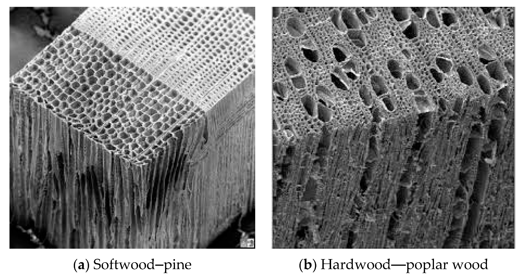
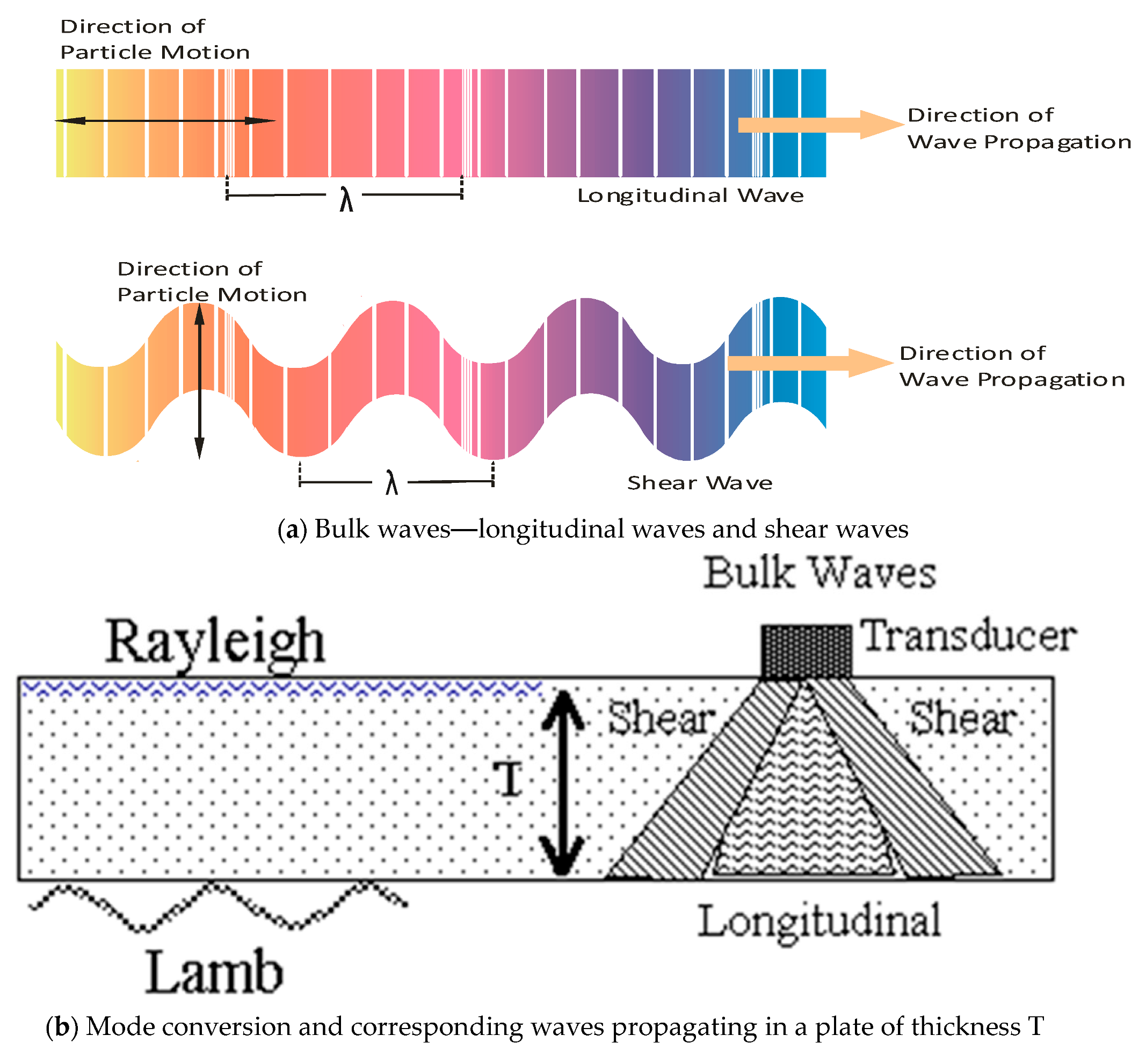
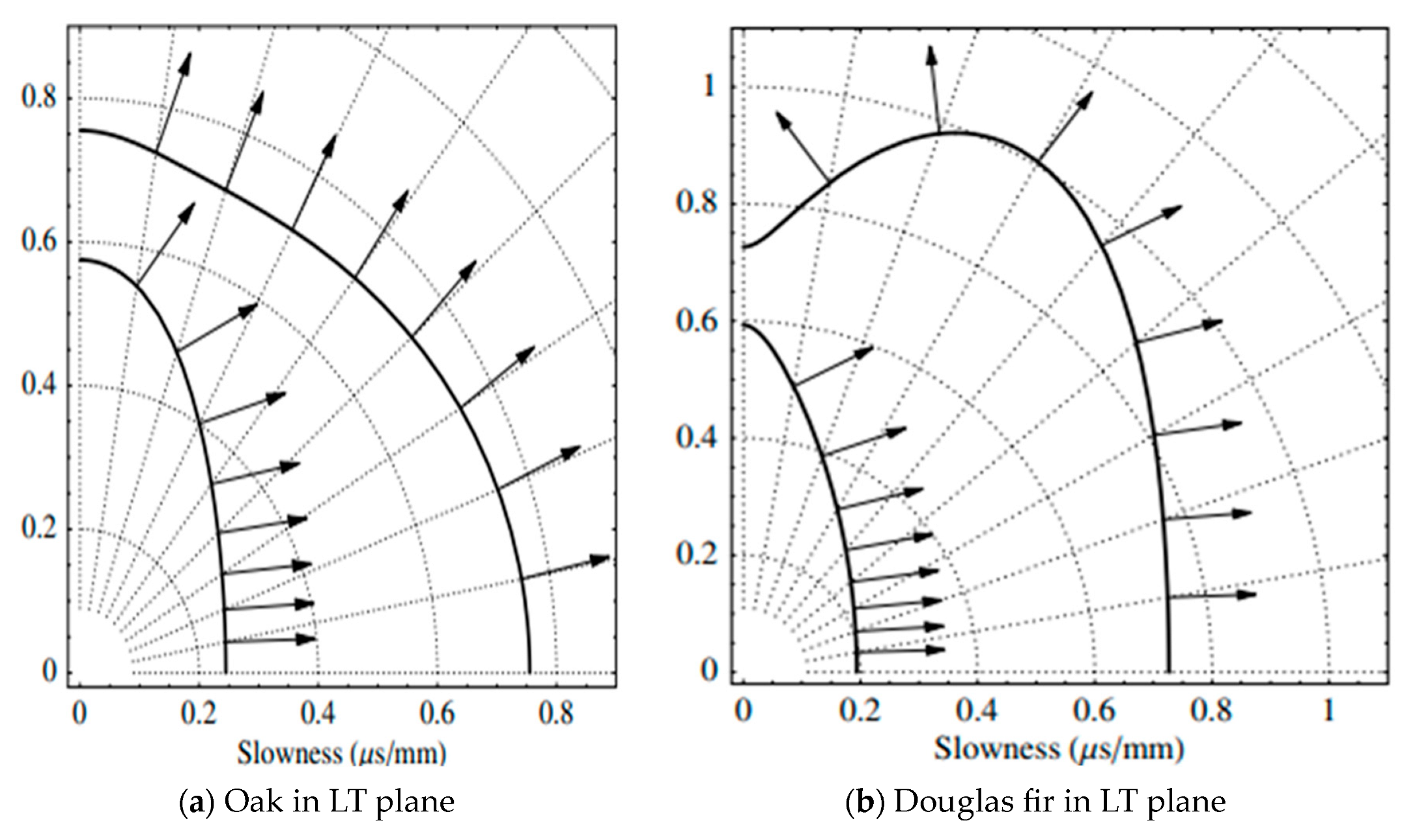
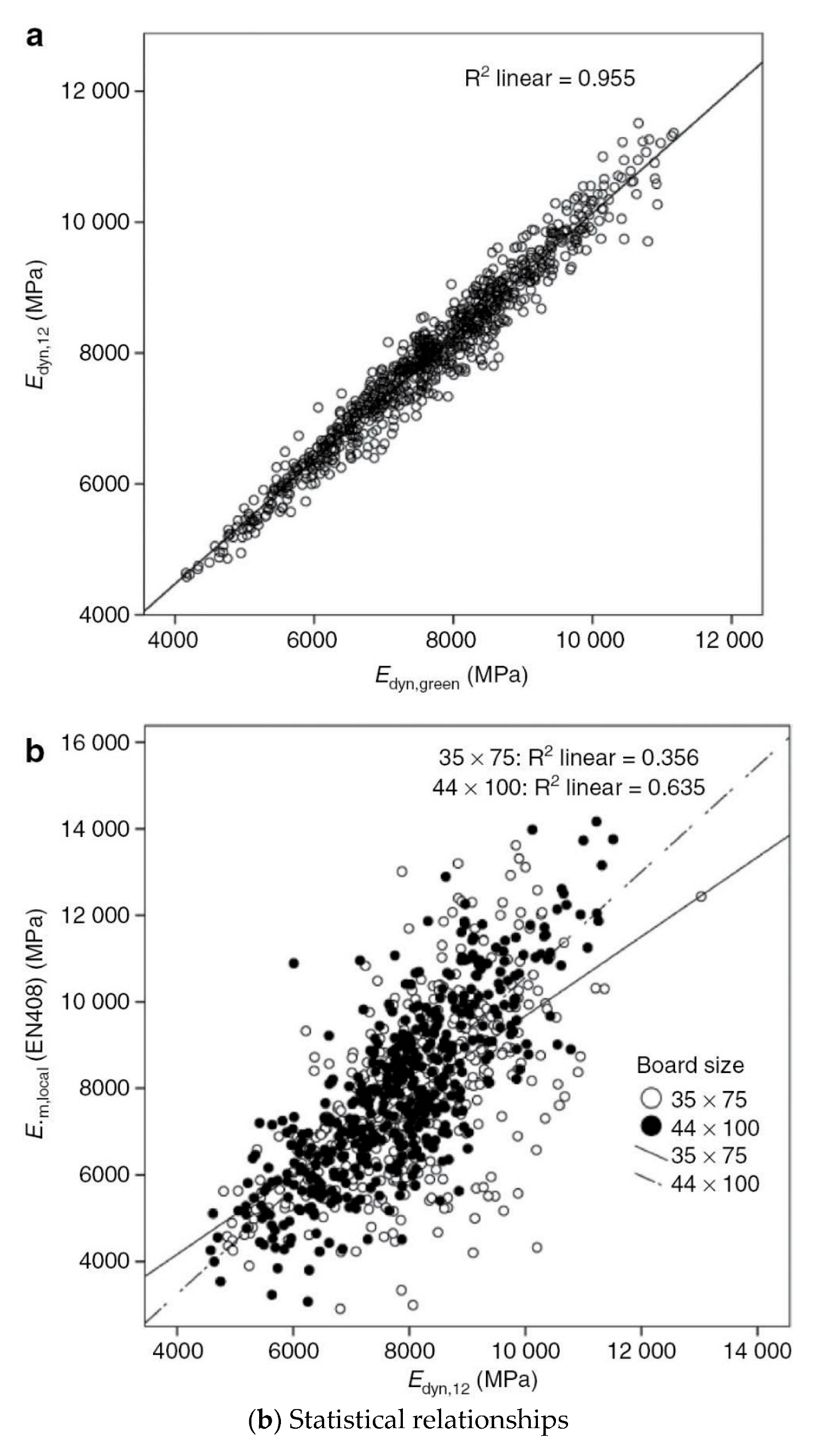
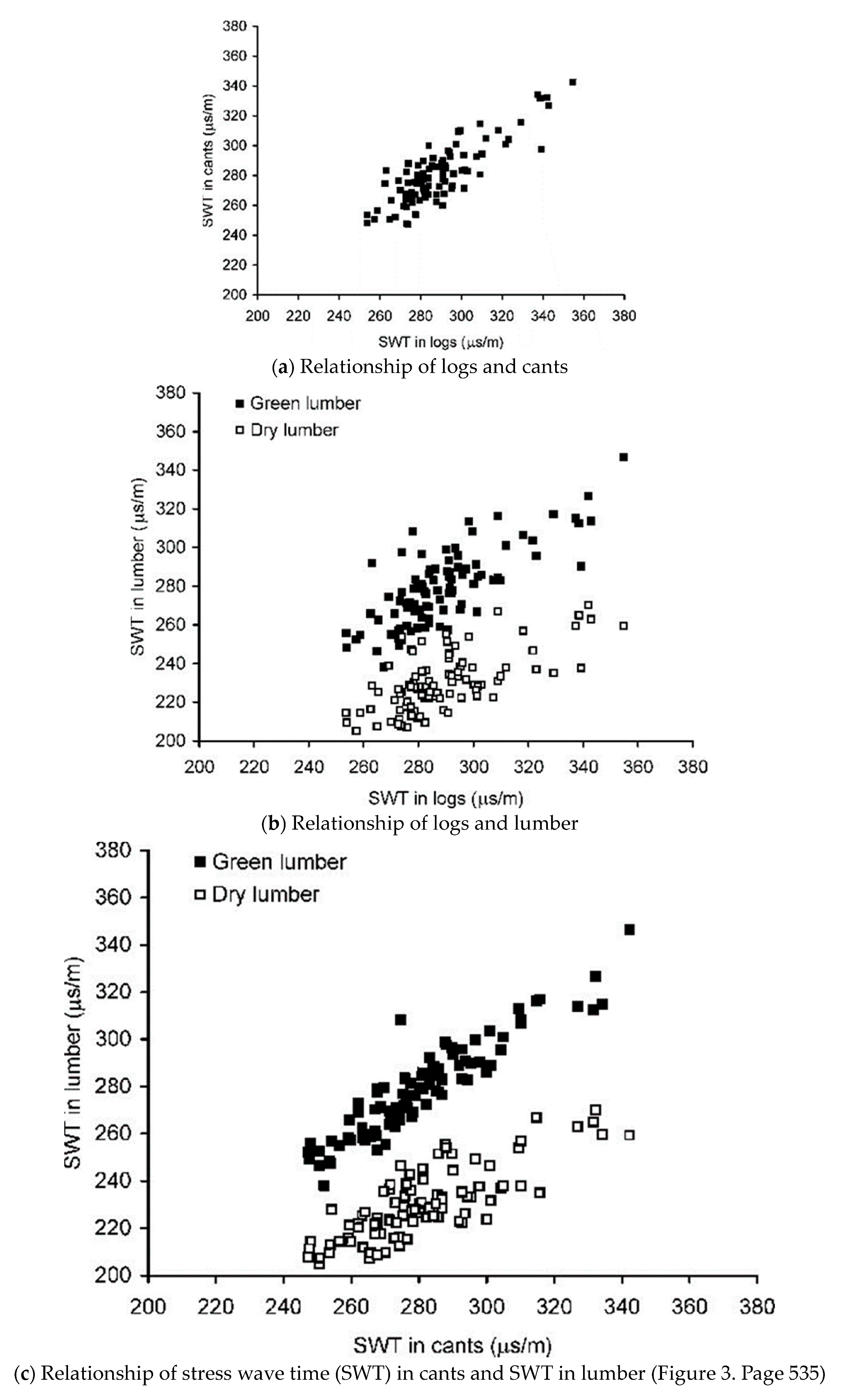
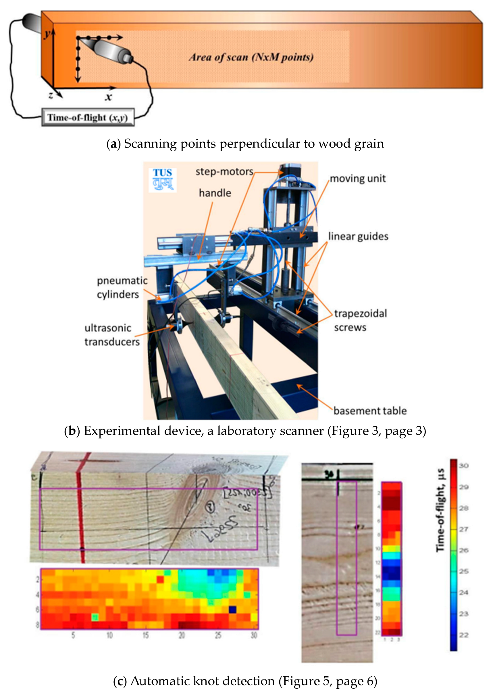
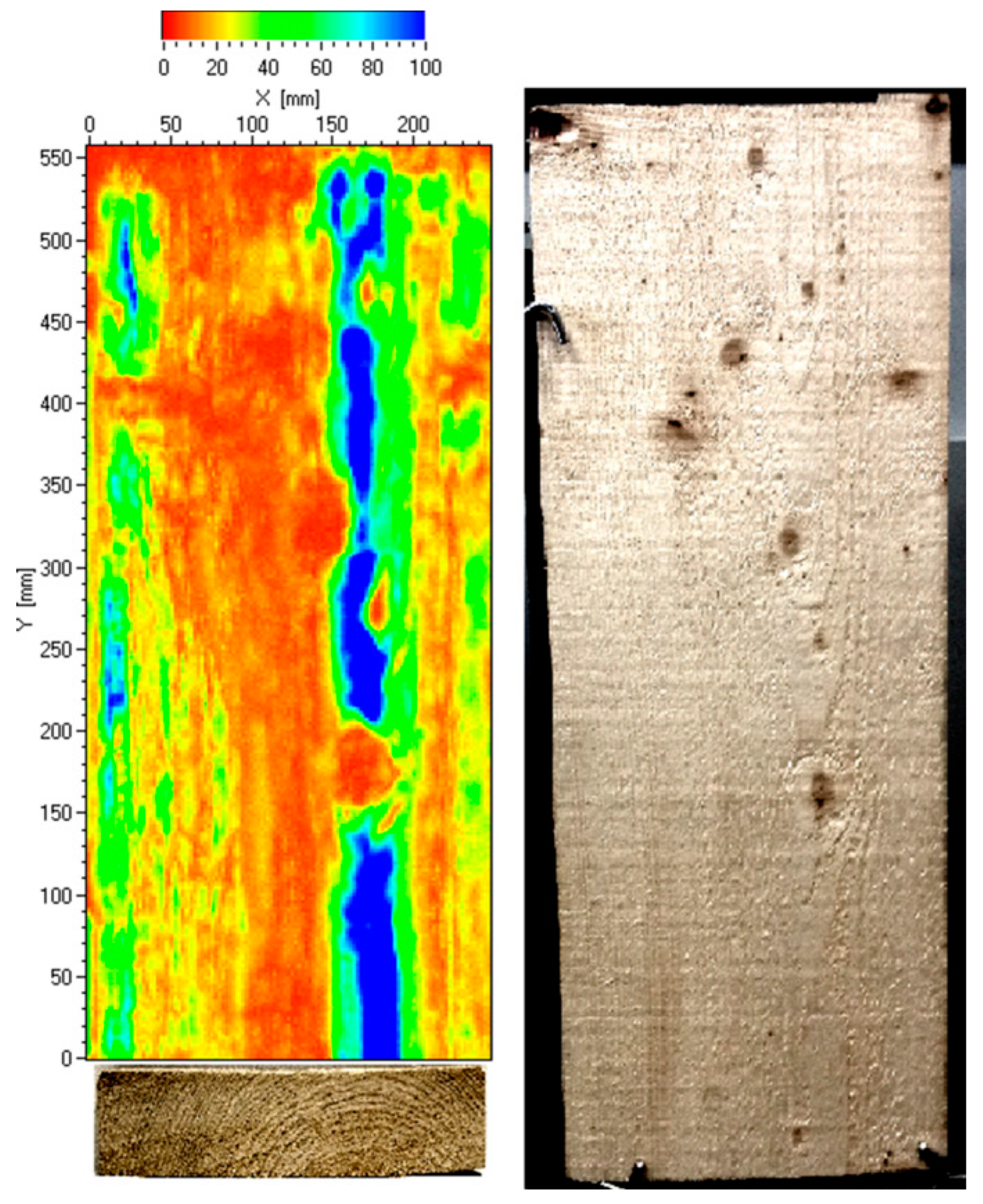
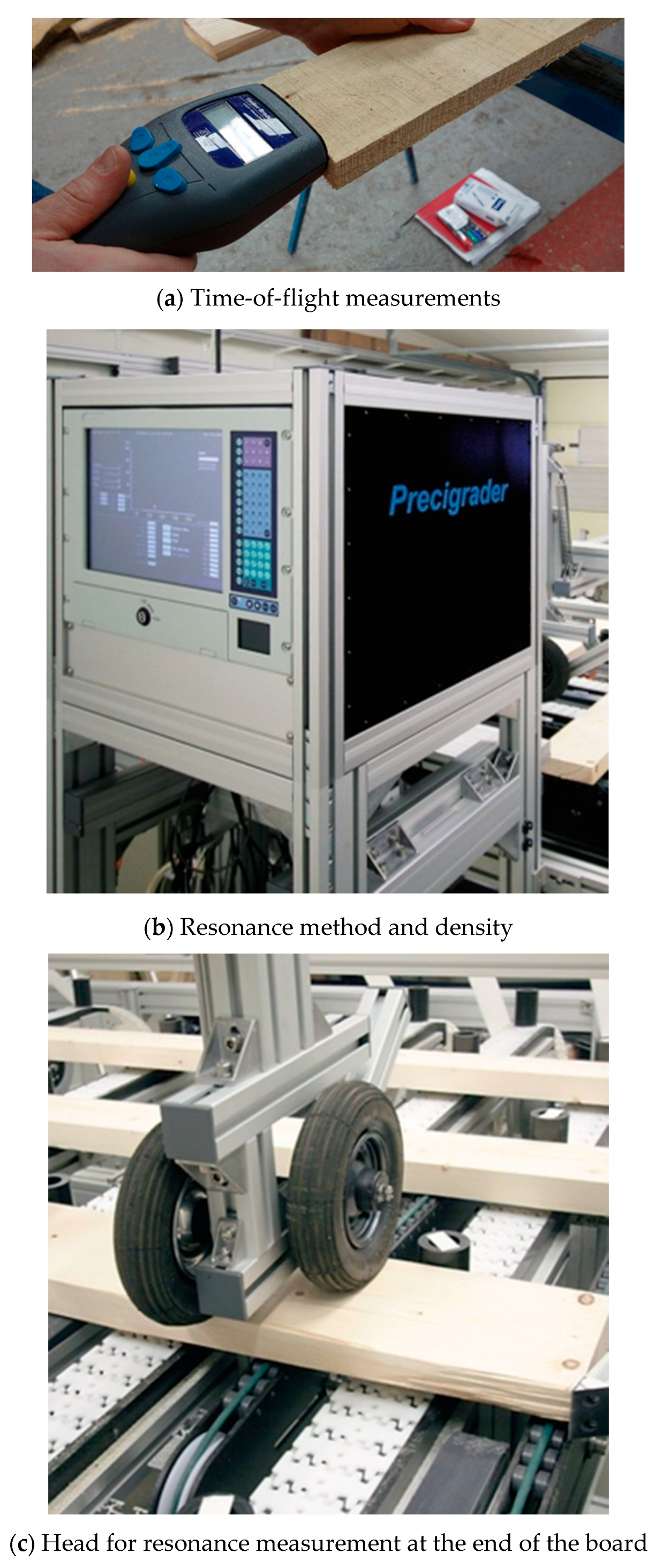
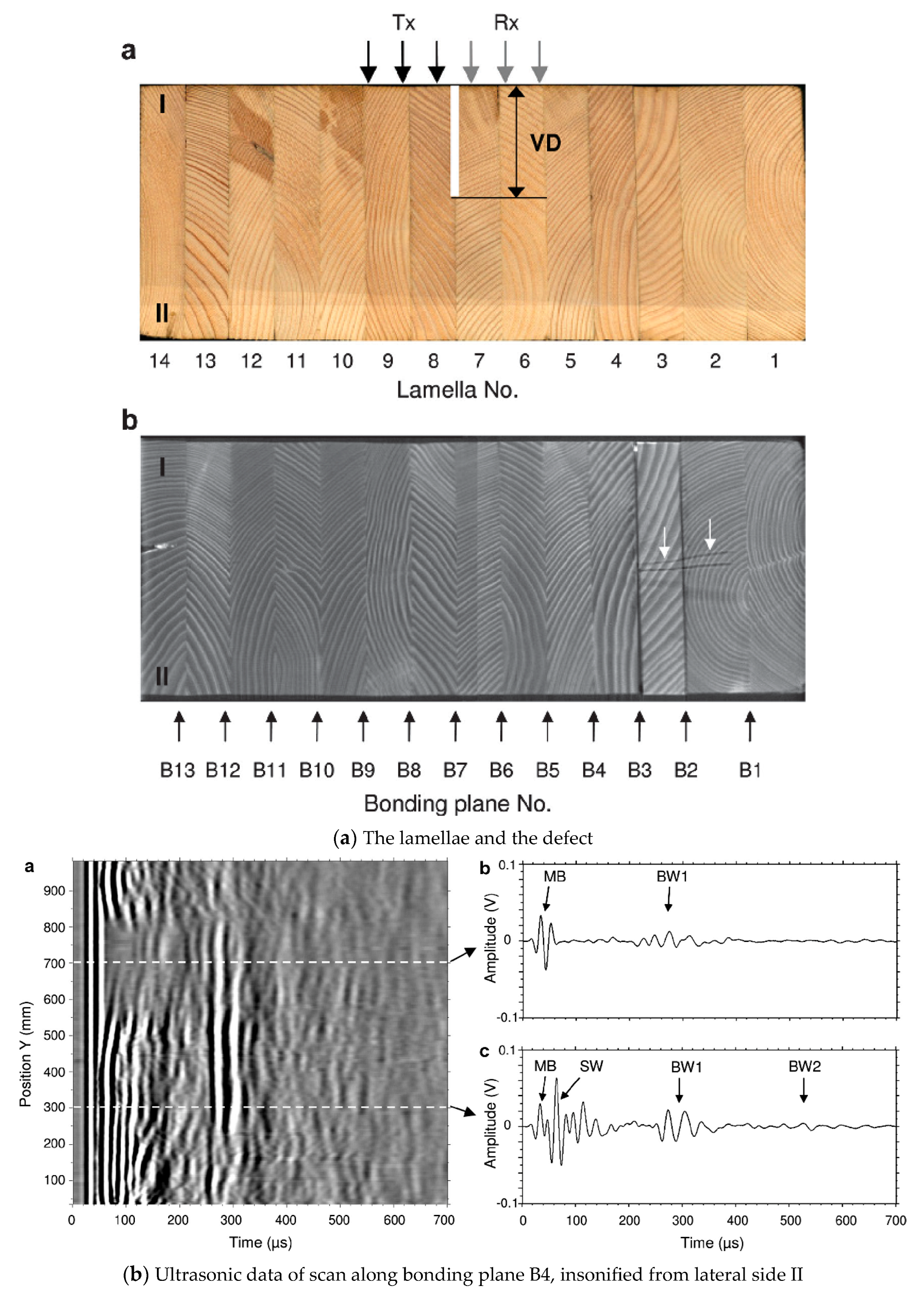
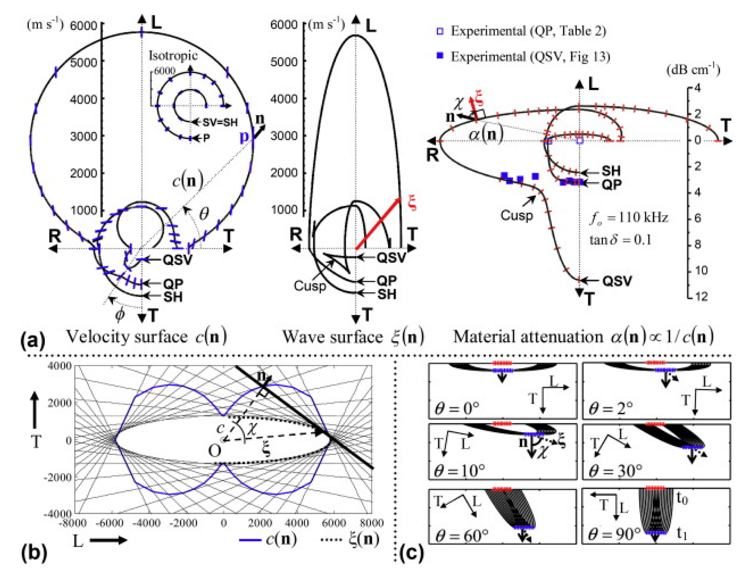
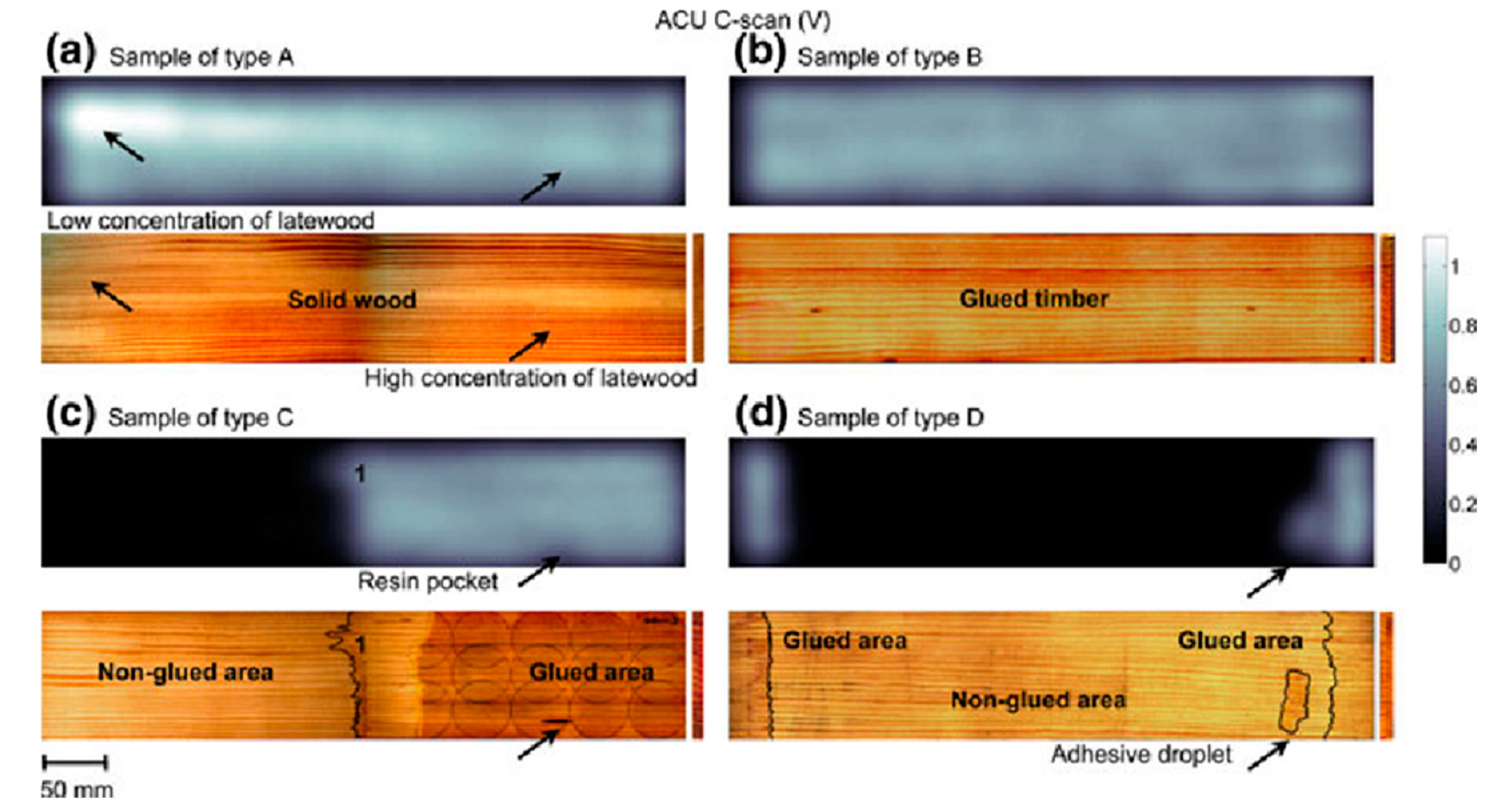
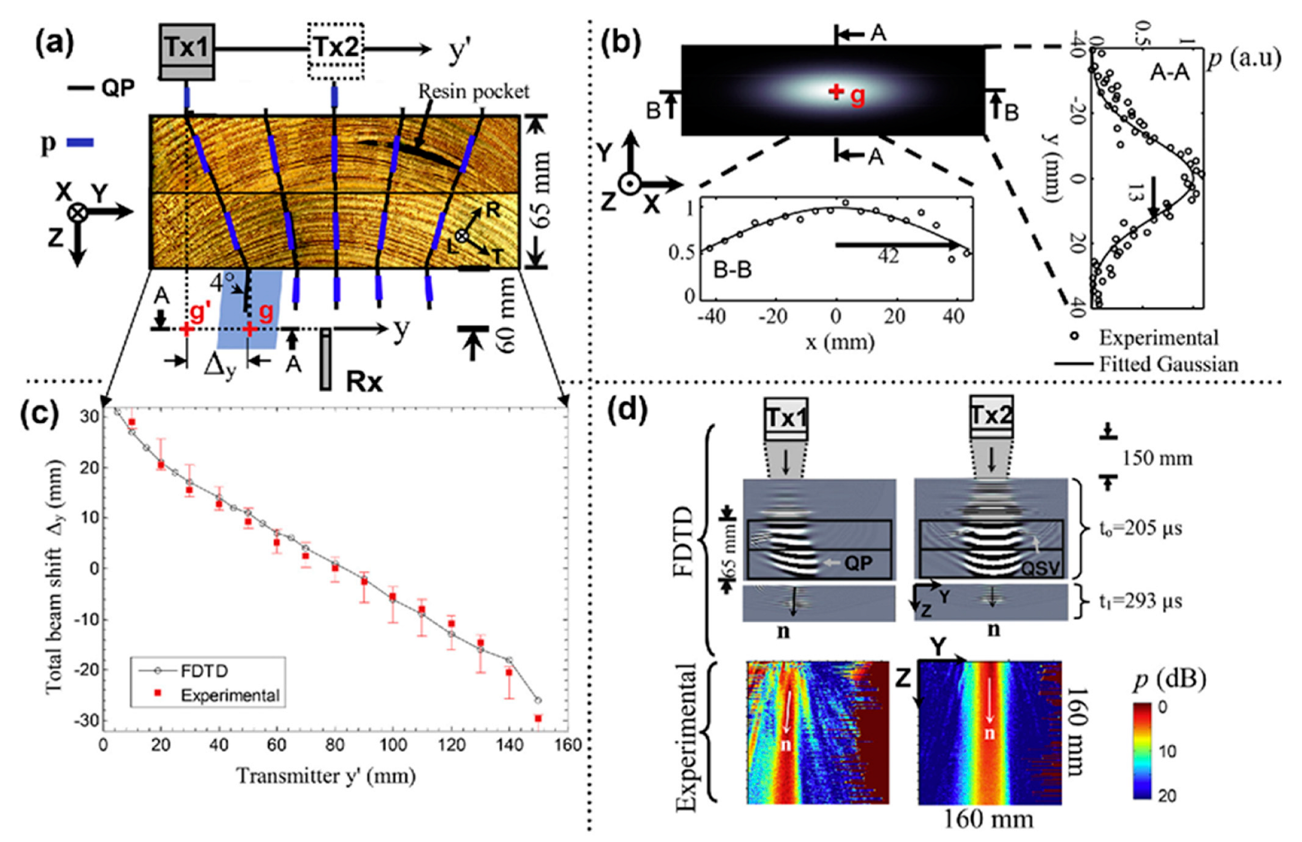
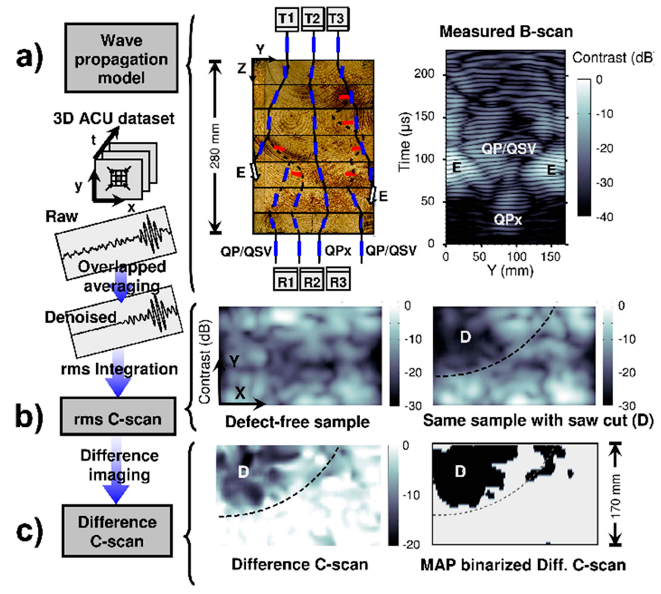
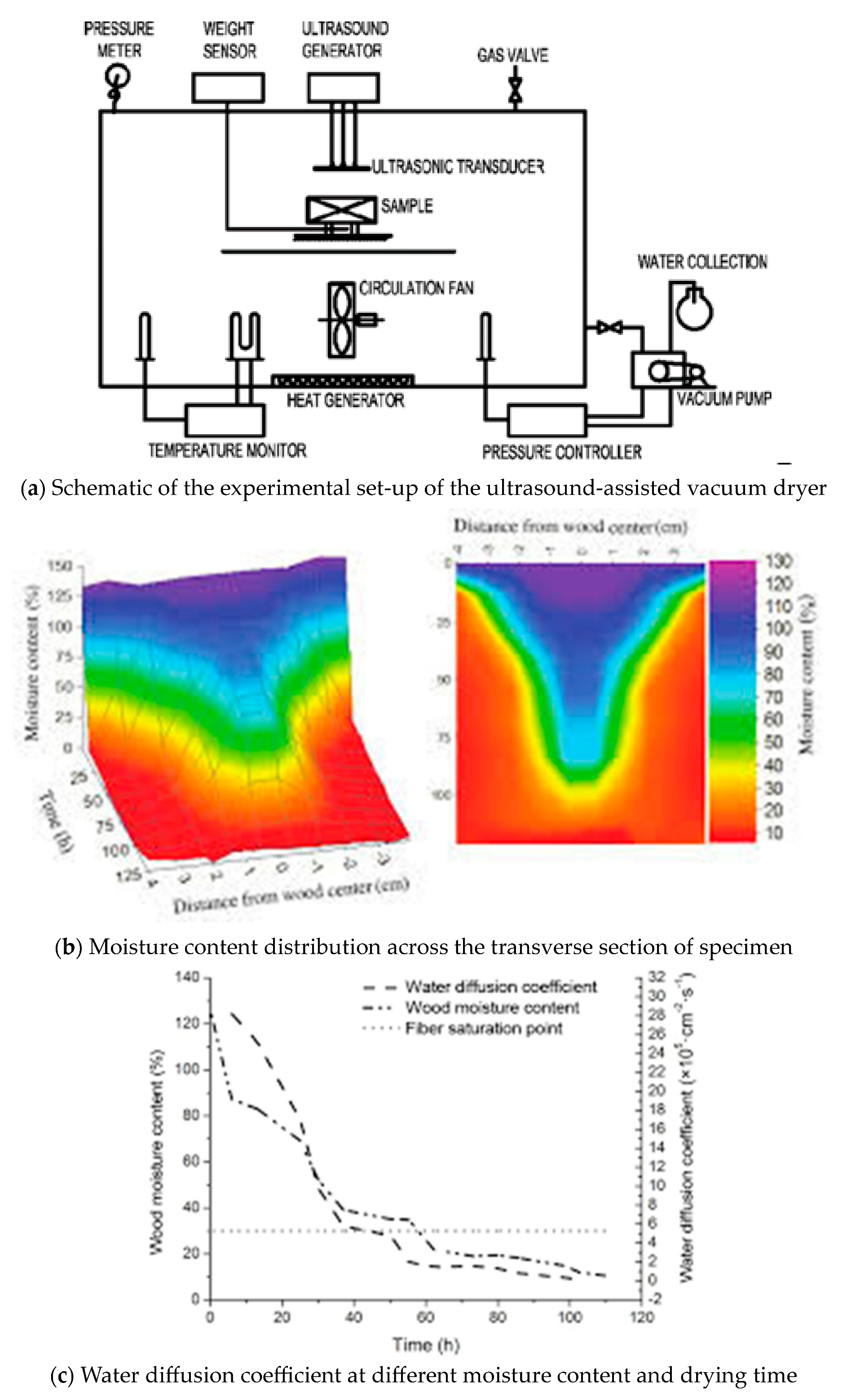
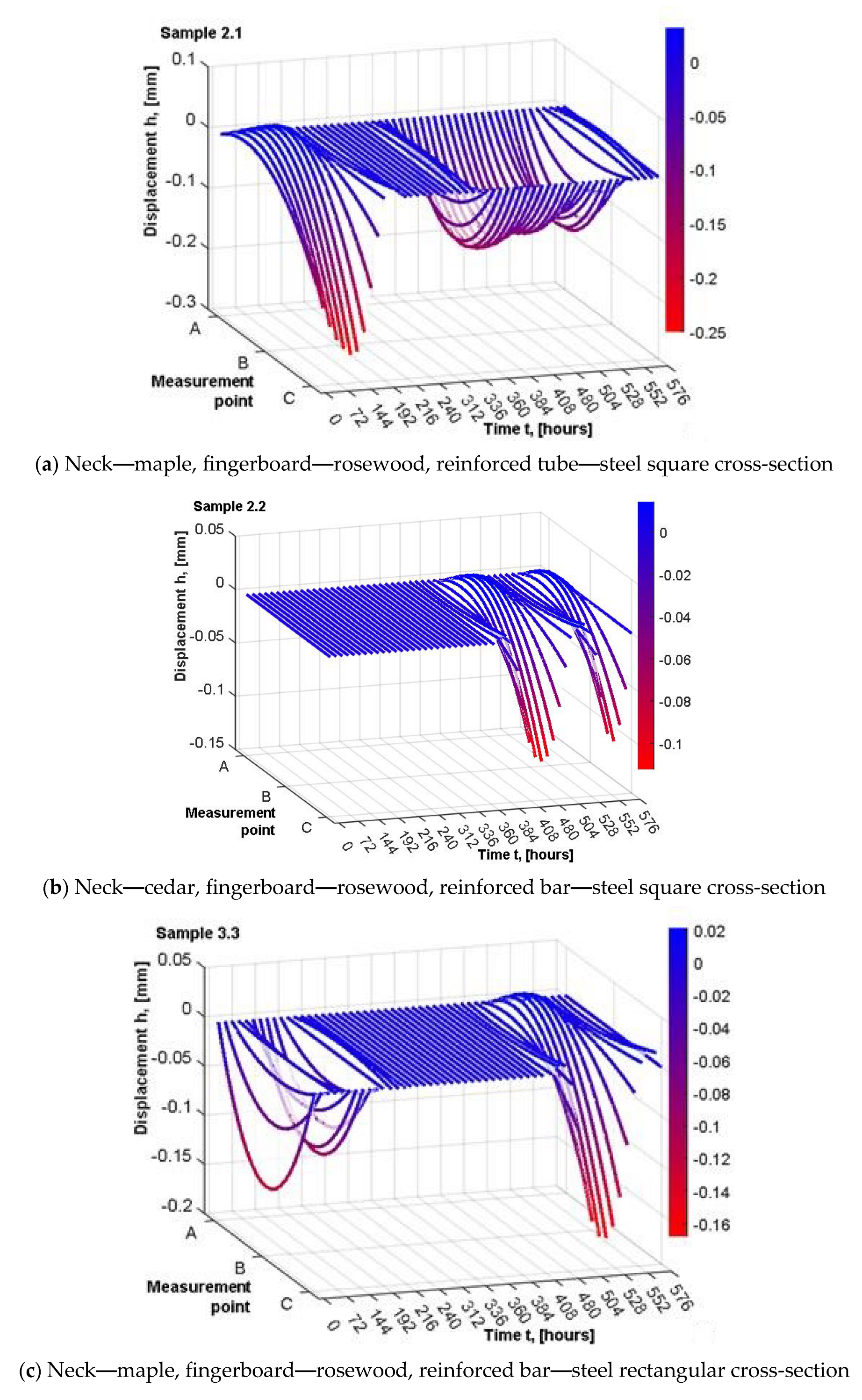
Table 26.
Acoustic technology for grading of boards [115] (data from Edinburgh Napier University, UK, https://blogs.napier.ac.uk/cwst/grading-machines-speeds/ accessed on 21 October 2021).
Table 26.
Acoustic technology for grading of boards [115] (data from Edinburgh Napier University, UK, https://blogs.napier.ac.uk/cwst/grading-machines-speeds/ accessed on 21 October 2021).
| Acoustic Method | Parameters Measured | Maximum Feed Speed | Company |
|---|---|---|---|
| Pieces/Min | |||
| longitudinal resonance | dynamic stiffness, without density | 100–240 | Dynalyse AB, Sweden |
| longitudinal resonance | dynamic stiffness, without density | 180 | Viscan (ViSCAN) Italy |
| longitudinal resonance combined X-ray | dynamic stiffness X-ray density, knots size and position | 150 –acoustic 80–300 X-ray | EuroGrecomat-706, Italy |
| longitudinal resonance | dynamic stiffness with density | manual operation | MTG 960., The Netherlands |
| longitudinal resonance | dynamic stiffness with density | 180 | Precigrader Dynalyse AB, Sweden |
| longitudinal resonance, combined optical scanner for knots | dynamic stiffness with density | 25 and 180 | Grademaster Illertissen, Germany |
| flexural resonance | dynamic stiffness with density | 20 | Xyloclass, France |
| edgewise flexural resonance | dynamic stiffness with density | 4 | SARL Esteves, France |
| ultrasonic time of flight, and pin indentation density | dynamic stiffness with density | 30–40 | Triomatic, France |
Figure 23.
Acoustic technology for lumber grading. Legend: (a) Acoustic technology for time of flight measurement at the end of the board [116] (https://blogs.napier.ac.uk/cwst/wp-content/uploads/sites/23/2016/12/DSC04840-e1480930831237.jpg) Accessed on 26 January 2022 (b) Resonance method and density© Limab Oy [117] (https://sahateollisuuskirja.fi/wp-content/uploads/precigrader_3_13_3_2_square-compressor-330x331.jpg). (c) The measurements are taken from the end of the boards at the processing speed. © Limab Oy [118] https://sahateollisuuskirja.fi/wp-content/uploads/resonanssivarahtelyn_mittaus_3_13_3_3-compressor-330x330.jpg accessed on 26 January 2022.

In Mediterranean countries, the sweet chestnut (Castanea sativa Mill.) is used traditionally as a structural element for construction. Machine grading can improve the utilization of this native resource. Ref. [119] studied the efficiency of machine grading according to European standard EN 14081-2 [93]. The grading parameters were the natural resonance frequency (by means of the industrial device—ViSCAN) and the corresponding dynamic modulus of elasticity and the static modulus of elasticity in four-point bending tests. With the assignment of EN 338 [120], some pieces by machine grading with the resonance method can be reclassed from class D to the higher class C for better utilization of the raw material in construction.
4. Acoustic Methods for Quality Assessment of Structural Composite Timber Products and of Wood-Based Composite Boards
The bulk of evidence in the literature refers to structural composite timber products and to wood based composite boards. The aim of this section is to produce a general overview on their characteristics.
4.1. The Background, LVL and Glulam
Structural composite timber products are highly engineered composites manufactured from wood. These composites highly improve the way in which wood should be used in structural applications. In the last decades, the importance of assessing large timber structures has grown considerably. The performance of these elements depends on the quality of the components, the quality of the finger joints, the quality of the glue-lines and the integrity of the cross-section of the structure [121]. These products are made of veneer—laminated veneer lumber (LVL)—or are made from lumber—glued laminated timber (glulam) or cross-laminated timber. For these products, all laminae are rated with acoustic methods before the assembly is bonded with highly durable adhesives. The laminae should be well aligned with the longitudinal axis of the final product. Figure 24 illustrates an LVL structure and a curved glulam beam. The main defects in glulam are illustrated in Figure 25. Anisotropic shrinkage and the growth stresses, the in-service moisture content gradient all contribute to the delamination of wood products. Swelling—shrinking stresses combined with mechanical stresses and in-service fatigue—either initiates or worsens the delamination. The causes of in-service failure of structures made of LVL or glulam have several aspects: the size and the natural defects (knots, compression wood, etc.), the shape and the orientation of the wood elements in the structure and adhesive curing and its interaction with the structural wood element [122].
Softwood and hardwood species are suitable for the production of LVL. The wood species most commonly used in North America are Douglas fir, larch and southern yellow pine. In Europe, spruce is the most common species for the glulam. LVL can be 1.2 m wide and 24 m long. The thickness of the dried veneer is 4 mm. The first commercial system ultrasonic veneer grader was installed in 1977, in Oregon, USA [124], with a production speed of 30.5 m/min for Douglas fir veneer, sorted into three grades. An ultrasonic method was used for the measurement of the propagation time in the longitudinal direction of lamellae, corresponding in fact to the L anisotropic direction of wood. Later, the density of each piece was determined and the modulus of elasticity was calculated. In the US, the company Metriguard developed ultrasonic equipment with production speeds from 91.4 to 129.5 m/min, with wood temperature compensation, radiofrequency measurement of specific gravity and moisture content, sheet width and with thickness detection capabilities [125].
Glued laminated timber products (glulam) are manufactured in rectilinear or curved shapes [126]. For glued laminated timber the thickness of the laminae should be smaller than 2 in (5 cm) and may include end- and edge-glued lumber. At the time of frame fabrication bending in a curved form is possible and permitted under existing regulations for construction. For glued laminated timber, grade requirements are specified for each lamina designated to be used in certain sections of the finished beam (inner or outer region under tension or compression).
A reliable bonding quality assessment of the glulam is necessary to reduce security hazards and maximize the life span of wooden construction. The choice of the adhesive type takes into account the moisture content of the wood and the climatic conditions of the building or of the environment in which the beam will be installed. For instance, polyurethane-based adhesives need a minimum wood moisture level during and after the gluing.
Another important factor during the service life of the beam is the effect of load duration, which can reduce the strength of the glulam. This effect is due to the variations of air temperature and humidity, which may lead to delamination and cracks of various sizes in the wood laminae. Therefore, to ensure safety of the building, a methodology for the full life cycle of a glulam should be developed for periodical testing of the integrity of the structure.
In glulam, two main types of defects are observed, natural defects in lumber like knots, splits, cracks, etc., and defects due to the adhesive. During manufacturing, defects in the glue line can be induced by inadequate pressing and curing parameters. These defects can be detected with non-destructive methods—X-ray, neutrons or acoustic methods like the stress wave method and the ultrasonic method. Computed tomography (X-ray, neutrons) methods based on non-refracting radiation (X-ray, neutrons) can detect the absence of adhesive in wood composites [127]. However, the hazardous nature of these methods still constrains their application on site.
Acoustic methods are nonhazardous. The stress wave method is based on the measurement of the time of a traveling stress wave generated by a shock with a hammer. Ultrasonic methods are sensitive to delaminated interfaces due to the quasi-specular wave reflection at the interfaces. The equipment for glulam beam inspection for direct contact ultrasound is portable and not very expensive [128]. The coupling of energy between transducers and sample needs a coupling agent. However, this aspect can be overcome with air-coupled ultrasonic transducers [129,130,131].
The direct contact ultrasonic technique in wood is affected by the anisotropy of the material, the strong attenuation and some experimental factors. The propagation of ultrasonic waves in wood may be attenuated by three main factors: the geometry of the radiation field, scattering and absorption. The first factor is related to both the properties of the radiation field of the transducer used for measurements (beam divergence and diffraction) and wave reflection and refraction occurring at the macroscopic boundary of the medium. These factors are related to the geometry of the specimen. Scattering and absorption are phenomena related to material characteristics. These aspects related to the direct transmission technique with the transducers in contact with the specimens have been discussed by [88,132,133,134].
4.2. Stress Wave Timing Inspection of Glulam Beams
Stress wave timing inspection of glulam beams was the firstly developed technique used for field inspections of large structures by Hoyle and Pellerin [135] Forest Products Laboratory—Madison Wis. USA. Figure 26a illustrates the equipment used and the experimental points of measurements on a glulam beam. The experimental measurements of the time propagation of the stress wave can be determined on structural elements oriented in the R direction, the T direction, at 45° or at another angle (Figure 26b). The effect of grain orientation on glulam nondecayed product made of Douglas fir, 12% MC is shown in Table 27. The measured time of stress wave propagation varies with the distance, but it is better to refer to the corresponding values of velocities of the velocities measured in the R and T directions and at 45° (Figure 26c).
In fact, we understand from the plane wave theory and for the L, R, T orthotropic model of wood elasticity that the R and T directions propagate pure longitudinal waves. The values of the velocities are: VR around 1490 m/s and VT around 1250 m/s. There is a mode conversion at 45° where there is the propagation of a quasi-longitudinal wave, the velocity is around 1000 m/s. The sound field was shifted from the insonification axis as a function of annual ring angle. The zones of the decayed wood will be easily detectable by lower values of velocities.
Progress in the technology of fabrication of transducers for ultrasonic inspection of composites allowed the development of new techniques for the control of structural elements made of timber with two main techniques, namely dry-point-contact ultrasound and air-coupled ultrasound.
4.3. Glued Laminated Timber Scanning by Dry-Point-Contact Ultrasound
The quality of adhesion by dry-point-contact ultrasound is assessed using the measurement of the time of flight through different zones of the glulam structure. The methodology for glulam timber scanning by dry-point-contact ultrasound was developed by [137] on specimens extracted for a beam in service for 90 years in an aircraft hangar in Lucerne in Switzerland. The glulam was made of spruce and the adhesive was casein-based (Figure 27). Dry-point-contact transducers were used in conjunction with a mechanical scanner to inspect this structural element. Pulse echo measurements were performed with a shear wave array comprised of 24 transducers of 50 kHz, grouped as transmitters and receivers. A specific scanning system was developed to perform automated defect imaging in glulam. Figure 28a shows the cross section of the sample, the position of the 14 lamellae, the position of the induced defect VD and the position of the transducers—emission and reception.
The identification of the ultrasonic echo is shown in Figure 28b. In the case of good bonding wood adhesive near the surface, the surface wave SW can be detected Figure 28c. We can also see the echoes BW1 and BW2.
Figure 28c displays the correlation between the ultrasonic surface echo amplitude with the delamination depth measured using a feeler gauge for three different bonding planes. The continuous curve reflects the main trendline. It was determined by using a clustering algorithm (20 consecutive points). The numerical simulation of wave propagation as a function of delamination depth in coordinates of ultrasonic attenuation versus delamination depth (Figure 28d) shows the efficiency of surface waves in detecting delamination to a maximum depth of about 55 mm. The back-wall echo BW1 is able to detect delamination to a depth of about 150 mm. It was concluded that the point contact technique described is suited for the detection of delamination in glulam. A delamination depth of 20 mm reduces the surface wave amplitude by about 20 dB. This value is beyond amplitude variations due to the natural variability of wood, which is about 15 dB.
4.4. Air-Coupled Ultrasound Inspection of Glued Laminated Timber
One of the factors affecting the air-coupled ultrasound inspection of wood is the energy flux deviation. Due to the anisotropic nature of wood, there is ultrasonic energy flux deviation, with mode splitting and phase shifts.
Air-coupled ultrasound inspection of glued laminated timber was possible due to advances in the technology of fabrication of transducers for non-contact ultrasonic inspection of materials [138].
For glulam beams, air-coupled ultrasound inspection (ACU) was developed by [130,131] based on the theoretical analysis of the normal transmission mode and on the development of signal processing algorithms applied to the imaging of bonding defects in multilayered glulam beams. Three cases have been analyzed: one unbonded wood lamella, two layers of glulam with bonding defects (the case of two lamellae) and several layers of glulam with a saw-cut defect (the case of 7 lamellae). The glulam is made of spruce, which has the characteristics mentioned in Table 28.
- (a)
- A single, unbonded timber lamella with curved growth rings in RT plane
The pioneering work on the path of ultrasonic waves propagating in a timber glulam structure by [123] developed a finite difference model in the time domain which incorporates the following parameters: the wood stiffnesses and their local variations, the damping of ultrasonic wave and the density of wood. Ultrasonic wave propagation in wood was studied and explained with a time-varying wavefront in unbounded timber with curved growth annual rings. The following properties of the air-coupled ultrasonic beams were studied: the velocity, the attenuation and beam skewing. In the cross-grain plane (RT) beam skewing leads to a position dependent wave path. Anisotropic damping in the RT plane is explained in terms of stiffnesses and a constant loss tangent. The attenuation coefficient was defined as α = π (f/velocity) tan δ. It was pointed out that tan δ varied very little in the range 0.09 to 0.13, on average tan δ = 0.1 for longitudinal waves propagated in the in RT plane and for the frequency f = 100 … 1000 kHz. This means that we have a constant attenuation per wave length factor α λ with the wavelength λ = velocity/frequency. This is a physical parameter of the hysteretic damping and leads to the linear frequency attenuation law.
In the RT plane, for frequencies 0.10 MHz and 0.25 MHz, [88] reported constant values of the ultrasonic attenuation longitudinal waves measured on horse chestnut (Aesculus hypocastanum) specimens with density 510 kg/m3 at a 12% moisture content. For higher frequencies than 1 MHz, there is an important effect caused by the anatomical structural element on attenuation values (horse chestnut is a species of high anatomical homogeneity).
For better understanding of phenomena related to the propagation of the air-coupled ultrasonic waves in glulam it is necessary firstly to note the ideas related to the wave propagation in unbounded timber in all anisotropic planes of wood.
We know that the plane wave front solution in an anisotropic medium is given by the Christoffel equation (Equation (18))
where δ ik is the Kronecker delta 1 = or 0
Eigen decomposition leads for each eigenvector n to three non-trivial roots for three velocities associated with three mutually orthogonal polarization vectors p.
In what follows, our attention will be focused on the following aspects related to wave propagation into the layered structure of the glulam:
- -
- The velocity surface, the wave surface and the attenuation in three anisotropic planes of solid wood;
- -
- The effect of the annual ring in a multilayer glulam;
- -
- Air-coupled ultrasonic wave propagation in a glulam structure composed of several lamellae.
- (b)
- Velocity surface, wave surface and attenuation in three anisotropic planes of solid wood.
The velocity surface, the wave surface and the attenuation in three anisotropic planes of solid wood are shown in Figure 29.
In the case of one of the most anisotropic wood species, i.e., spruce, Figure 29a shows the velocity surface, the wave surface and the attenuation in three anisotropic planes. The energy flux vector ξ is perpendicular to the slowness expressed as 1/velocity (n). The skew angle χ is the inclination between n and ξ. The material attenuation surface is α (n). We have in compact representation the velocity surface V(n) or as noted in the graph c(n) for the planes LR, LT and RT and the corresponding pure longitudinal waves along the axes (p//n) and pure shear wave (p n). The variation of the propagation angle generates in one plane the following three waves: QP—quasi-longitudinal wave, QSV—quasi-shear wave and pure SH—shear wave polarization perpendicular to the plane. On the same graph is represented the case of aluminum, a solid considered as isotropic, having VL = 6000 m/s, compared to spruce having VLL = 5500 m/s. Wave surface is represented as the variation of the energy flux vector ξ (n), which is the outward power flux through the point wavefronts (Equation (19))
Due to the anisotropy, the wave is shifted by a skew angle χ from n.
The polarization, p, is plotted on the velocity surface with respect to the wave normal n.
Figure 29b illustrates the geometrical construction for the wave surface ξ (n) and the energy flux shifts χ for the fastest mode in the LT plane. ξ (n) is the envelope of the plane wavefront radiating in all directions n from a point excitation O. Figure 29c shows the effect of the grain angle Θ by decomposing the beam at time t = to in elementary sources and calculating their envelope at a later time instant t1.
- (c)
- the wave path in a structure made of two lamellae
Figure 30 illustrates the wave propagation path in a glulam sample made of two lamellae. The characteristics of the path wave in the RT plane of a single timber lamella are shown in Figure 30a.
The theoretical analysis was based on the theoretical model of the main wave propagation paths and the impact of wood anisotropy on the lamination assessment. Figure 30a illustrates the position of the transmitter and receiver, the pathway in a lamella of thickness d composed on n layers of annual rings and the anisotropic axes R and T of wood. In this structure quasi-longitudinal (QP), quasi shear (QSV) and pure shear waves (SH) propagate simultaneously. The phase velocity surface and the mode definition in the RT plane are illustrated in Figure 30b. The variation of the ring angle orientation from 0° to 90° in the RT plane determines the variation of the flux energy.
The shift of flux energy versus ring angle is shown in Figure 30c. In the principal material axes R and T, all modes propagate aligned with n. One observes that there is an intersection between QP and QSV at around 30°. The QP mode tends to align with T and R with an equilibrium point at Φ = 30°. (pure P mode). This is an equilibrium point. The energy flux shift of QSV varies between −60° to +60°. The shear wave is affected very little by the variation of the annual ring angle Φ°. There is a wave surface cusp at Φ = 39°, which aligns ξ and n.
The transmission coefficient T (air, wood) and T (wood, air) is shown in Figure 30d and corresponds to the coupling losses for specific modes. In other words, the losses are also equivalent to the maximum amplitude reduction observed when the ultrasound is transmitted through a delaminated interface compared to defect free glulam. We can see that only QP and QSV are coupled. SH is not coupled. QP is affected very little by the variation of the angle, while QSV has a huge variation between about 35° and 90°. For spruce, the velocity of QP the quasi-longitudinal wave is between 910 and 1270 m/s and the velocity of the shear mode SH is between 1130 m/s and 1260 m/s, except in the vicinity of R. The QSV is the slower mode with a velocity between 280 and 620 m/s. In the axes R and T, the pure P wave and SV modes are coupled. Due to the ellipticity of the velocity surface, the energy flux ξ deviates from the propagation vector n except for R and T, giving rise to a lateral shift χ (°). The ultrasonic field coupled into glulam diverges from the insonification axis Z and propagates along ξ, whose field is only partially captured by the receiver. The large lateral shift χ (°) results in strong energy losses. We can see that the energy flux shifts are highly dependent on the coupled mode and the angle of the orientation of the annual rings. For the pure shear mode SH, the lateral shift χ (°) is less than 6°; therefore, it can be said that the contact shear transducers polarized in the fiber direction perform best for glulam inspection.
Figure 31a illustrates the path wave in A scan mode in a glulam structure made of two lamellae, in a zone of glued area compared with a non-glued zone. Note 1 and 2 correspond to waves propagating through the sample, 3 is the signal corresponding to multiple reflections between the receiver, 4 is the waves blocked by the frame built around the sample and 5 is the multiple reflections in the damping mass of the transducer. The block diagram is shown in Figure 31b.
Visualization with ACU imaging in glulam corresponding to the glued area compared with non-glued area is illustrated in Figure 32 for the case of two lamellae.
A more complex analysis of the propagation paths in the glulam structure is shown in Figure 33. The wave propagation paths are nominally invariant along the grain direction (X and L) due to the laminate symmetry. The ray paths of the QP mode, which is dominant, varies with the transmitter position y′. Note the beam skewing effect which tends to orient the ultrasonic beam along the nearest material axis (axis R). The position of the radiated beam is shown in Figure 33b. Total beam shifts, both experimental and simulated, are displayed in Figure 33c. Simulated and experimental pressure field distributions are in the YZ plane with Rx for two transmitter positions Tx1 and Tx2 (Figure 33d). The choice of the distance dR between the sample and the transducer Rx is not critical because the radiated ultrasonic beam spreads slowly. The curvature of the annual rings is associated with the local gradient of the stiffness, which can be observed with the kinematics of the flux energy ray tracing.
- (d)
- The wave path in a structure made of seven lamellae
The effect of the annual ring in a multilayer glulam introduced supplementary difficulties for the modeling of the path of the ultrasonic wave. Each lamella has its own annual rings oriented differently. Figure 34 explains the effect of the annual ring on the modeling in a multilayer glulam through the coordinate transformation of wood material LRT in sample X-Y-Z coordinates as a function of grain angle Θ and ring angle Φ.
u = AE AL u′ = Au′
The approach was based on:
- -
- The coordinate transformation with respect to the pith of the tree, for a cylindrical stem model, for the analysis of vibration modes in a defect clear specimen.
- -
- The calculation of the elastic properties of the glulam
A glulam is described by projecting the displacement fields u′ in the L, R, T coordinate system of each lamella to a common Cartesian system u (X, Y, Z). X corresponds to lamella length, and Y and Z correspond to the height and depth. Two successive axes of rotation AL and AR are in terms of the ring angle Φ (inclination between Z and T for Θ = 0°) and grain angle Θ (inclination between X and L) and define the transformation matrix u = AR AL u′ = Au′.
A cylindrical growth annual ring model allows computation of ring angle Φ as a function of the position of the pith P (y0, z0) of each lamella. An X-symmetric glulam beam can be determined by observation of the end surfaces of the composite
for
As noted by [131] “the 6 × 6 Bond Matrix M (aij) then allows the computationally efficient projection of Cij from u′ and u in terms of the elements a ij of the transformation matrix A with C = MC′MT”.
The model incorporated the adhesive, polyurethane, having a density of 1400 kg/m3 and velocities of 875 m/s and 378 m/s. The stiffness tensor in air was calculated for a velocity of 346 m/s and an acoustic impedance of 428 Pa s m−1 with Cij = 0.
The model proposed by [131] accurately describes the anisotropic wave propagation phenomena derived from the plane wave and point source analytical model. The density gradients (Figure 35) observed in the growth rings did not significantly influence beam skewing with respect to the homogenized model proposed.
Modeling for a more complex case is illustrated in Figure 36 for air-coupled ultrasonic wave propagation in a glulam structure composed of seven lamellae (280 mm) in which the wave propagation is less dependent on the Tx position. The wave paths crossing the structure QP/QSV, QPx and QP/QSV are specified in blue (Figure 36a). Note the refraction phenomena at the interface between the lamellae and at the specimen boundaries. The experimental and simulated data are consistent for the peak amplitude positions, corresponding to the re-radiation of the main wave propagation path. The simulation provides a “full history” of wave propagation related to the variation of the local density of the glulam, incorporating the heterogeneity of the material. Ref. [131] demonstrated that the growth ring structure significantly influences the wave propagation in the anisotropic RT plane. A strong skewing effect was observed, up to 30° for longitudinal QP modes and 60° for quasi shear modes QSV. This effect shifts the ultrasonic beam from the refraction path. It is worth mentioning that if this effect is not accounted for, there is a fading effect of the signal at the receiver, which can compromise the ultrasonic technique even for glulam which is a few centimeters thick. The wave path with the B and C scanning mode was studied for the modeling of a structure with 7 lamellae having a 280 mm thickness, which gives a total of 8192 possible mode combinations (Figure 36b,c). The wave paths are
- -
- The first path having the QPx mode at the center of the beam.
- -
- The secondary paths having interference of the QP/QSV modes with small total shifts and edge reflection, E coupled at all sample width positions in the B-scan
- -
- in the RT plane and beam skewing leads to position dependent wave paths.
- -
- C-scan image of the structure without defect.
- -
- C-scan image with the delamination of a saw cut defect. Defects larger than 100 mm × 100 mm can be imaged. The maximum height of the glulam was 280 mm. Accurate segmentation of the geometry of the defect was obtained with a MAP binarization procedure described by [139].
- -
- For the 7-lamella system, a very complex QP/QSV interference pattern and edge reflections were identified and were imaged with the C-scan mode.
The curved pattern of the annual growth rings in the RT plane significantly effects the wave propagation path (see QPx propagating in R), inducing strong skewing effects (up to 30° for QP and 60° for shear modes QSV) that shift the ultrasonic beam from the refraction paths compared to the path calculated for isotropic media. This effect induces signal fading at the ultrasonic receiver. The finite difference time domain model based on the orthotropic stiffness dataset proposed by [131] combined with sound field imaging is an original and outstanding contribution to the understanding of phenomena generated by air-coupled ultrasound propagation in glulam structures and to the methodology for defect detection in situ.
5. High-Power Ultrasound
5.1. Introduction
High-power ultrasound or macrosonics is a branch of ultrasonics related to high-intensity ultrasonic waves (>1 W/cm2). The frequency of high-power ultrasound is between 20 kHz and 100 kHz. These high-power ultrasonic waves are able to modify the structure of the medium where they propagate. The propagation of high-intensity ultrasonic waves in media produces nonlinear effects associated with the finite high amplitudes. Nonlinear effects include wave distortion, radiation pressure, cavitation and dislocations, which can induce mechanical rupture, chemical effects, interface instabilities, friction, etc. All these physical effects can be employed to enhance processes that depend on the ultrasonic field irradiated into the medium. The successful application of high-power ultrasound is very much related to the transducers used and to the uniform distribution of the acoustic field within the processed medium. As mentioned by [140], the practical application of high-power ultrasonic techniques depends “on the adequate exploration of the effects linked to nonlinear phenomena produced during their propagation” The effectiveness of acoustic drying has been confirmed by the pharmaceutics industry and the food industry for heat-sensitive materials [141,142,143]. In wood technology, applications of high-power ultrasound are related to wood processing [2]. Current applications are for drying of lumber, drying of veneer [144], defibering [145], cutting [146], plasticizing [147], extraction improvement, regeneration effects on aged glue resins [148], welding [149] and wood preservation and sterilization. Because of space limitations, in what follows, attention is focused only on two main aspects: wood drying and wood sterilization.
5.2. Wood Drying
Interest in the development of acoustic drying techniques has been supported by the capacity of these techniques to rapidly remove the moisture content from materials without increasing the temperature and reducing the moisture gradient of boundary layers. During drying the moisture content of wood migrates from the center of the specimen to the periphery. It was demonstrated experimentally that high-power ultrasonic waves could have a very positive effect on the temperature gradient in the transverse sections of cylindrical wood specimens which are either air dried or fully water saturated [150].
In the wood industry, to the best of our knowledge, attempts to use ultrasound drying techniques were reported first in Australia. Recognizing the relative difficulty of drying Australian eucalyptus, ref. [151] proposed the use of ultrasound to reduce collapse during drying by impregnation with bulking or wetting agents. His approach was limited to laboratory testing and was based on the assumption that the effect of the surface forces developed during drying could be offset by the nucleation of bubbles inside the lumen of the cells. Ref. [152] proposed avoiding collapse in eucalyptus by heating the wood with ultrasonic energy. He tested boards (25 mm × 100 mm × 300 mm) with a commercially available welder, producing power of 750 W at 20 kHz. The rise in temperature at 150 °C and the contact pressure between the horn and the specimen at 140 kPa resulted in high shrinkage of the tested specimen and consequently its degradation. To avoid this effect a combination of pre-ultrasonic treatment with drying at low temperatures was proposed, but no commercially viable techniques were further reported.
The technology of wood drying can be improved with high-power ultrasound by two methods, namely by combining high-power ultrasound with infrared radiation or by combining high-power ultrasound with vacuum.
- (a)
- High-power ultrasound and infrared radiation
Based on laboratory experiments, [153] reported a procedure of wood drying specimens under high-power ultrasound combined with infrared radiation. Pine specimens of 2.5 cm thickness × 4 cm length × 1.5 cm width in saturated condition were submitted to a constant static pressure of 0.5 kg/cm2 and to various ultrasonic power levels.
The experimental setup for wood drying is shown in Figure 37. Ultrasonic energy is applied in direct contact with the specimens. The specimen is held between the stepped-plate power ultrasonic transducer and a flat plate parallel to the ultrasonic radiator. A suction pump removes the moisture and three pneumatic pistons ensure the mechanical coupling between the sample and the transducer. The infrared radiation source of 250 W was placed transversally to the samples. Figure 38 displays the decreasing moisture content in specimens, when high-power ultrasound (90 W, 60 W, 30 W and 20 kHz frequency) and infrared radiation (250 W) were applied simultaneously. Decreasing the moisture content from 100% to 12% in 30 min was possible using this combined method, compared to an ultrasonic high-power test at 90 W, in which the same size specimen needed 70 min to reach the same moisture content. The temperature measured at the surface of the pine specimen was between 35 °C and 45 °C. No damage was apparent at the surface of the samples. This is because below the fiber saturation point, which is about 30% moisture content for wood, diffusion of free water and bound water from the transverse section of wood specimens takes place quasi-simultaneously, with a slow release of free water.
At the level of fine structure of wood, at about the 10-micron scale, high-power ultrasonic wave propagation in wood induces structural modifications. Ref. [154] reported the effect of high-power ultrasonic treatment at a 20 kHz frequency on small saturated Douglas fir specimens. A significant increase in specific permeability coefficients in both the radial and tangential directions was observed. Permeability rate improvement was due to wood structural modification observed as the rupture of the pits’ margo/torus system in the cellular wall.
- (b)
- High-power ultrasound and vacuum
The combination of high-power ultrasound with vacuum had the main purpose of reducing drying time [155,156]. For experimental laboratory tests, the specimens were previously saturated in water. As mentioned previously, when the specimens were submitted to high-power ultrasonic waves, cavitation is produced and the fine structure of wood is destroyed at the pits level by the creation of structural micro channels which improve the permeability of the specimen. Ref. [156] reported experiments with specimens of poplar (Populus cathayana) submitted to high-power ultrasound of 40 kHz frequency for intervals of 30 min, 60 min and 90 min (Figure 38). The main effect of ultrasonic treatment is the rupture of fine structural elements such as pits and other elements. The diffusion of the moisture content from the center of the specimen to the periphery is improved by a “sponge effect” generated by the cavitation induced by the high-power ultrasonic waves. This effect increases the convective mass transfer into the specimen.
The effect of the duration of ultrasonic treatment for two frequencies, 28 kHz and 40 kHz, on water diffusivity of poplar specimens is illustrated in Table 29. Compared with the control specimen, the reduction of drying time is between 17% for 30 min of ultrasonic treatment and 26% for 90 min treatment with high-power ultrasound of 28 kHz frequency. The frequency effect is a time reduction of about 9.2% for a 40 kHz frequency compared to a 28 kHz frequency. The drying time of specimens pre-treated with ultrasonic waves decreases substantially compared to the control specimen. The factors affecting the drying time are the ultrasonic frequency and the duration of ultrasonic treatment. Comparing the effect of frequency, there is a decreasing drying time with increasing frequency.
Specimens of poplar (Populus cathayana) of a size currently used in the furniture industry (450 mm length and transverse section of 100 mm × 40 mm) were submitted to a high-power ultrasonic treatment followed by vacuum drying [156]. The experimental set-up of the high-power ultrasound treatment for vacuum drying equipment is given in Figure 39a and is composed of the following sub ensembles:
- -
- The ultrasonic sub ensemble is composed of a generator and of an ultrasonic transducer 66 mm in diameter, weighing 0.9 kg with a frequency 20 kHz and power of 100 W. The samples are in direct contact with the transducer.
- -
- The vacuum sub ensemble, where the air velocity is controlled by pulse modulation. Air velocity was set at 2 m/s.
- -
- The heating sub ensemble (the nature of the heating source is not specified). The temperature monitor and the heat generator were designed for a maximum achievable temperature of 200 °C. Wood drying temperature was set at 60 °C and the absolute pressure was set at 0.02 MPa.
- -
- The specimens’ initial moisture content 130%. The final moisture content of the specimens was 10%. Water evaporation is only from the surface of the specimen (450 mm × 100 mm). During ultrasonic treatment water migration is only along the thickness of the specimen, from the central zone to the surface.
- -
- The drying process was followed through the calculation of the water diffusion coefficient and by observing its variation during the drying time.
The effect of drying time on decreasing moisture content and the distribution of moisture content in the transverse section of the specimen are illustrated in Figure 39b. The variation of the water diffusion coefficient at different moisture contents as a function of drying time is displayed in Figure 39c. The increase in drying time from 0 to 125 h, is caused by the decrease in the water diffusion coefficient from 2.89 × 10⁻⁴ cm2s−1 for saturated specimens, to 3.02 × 10⁻⁶ cm2s−1 for a moisture content at the fiber saturation point, and to 2.27 × 10⁻⁷ cm2s−1 when the wood moisture content is 10%.
Water diffusion coefficient is a very useful parameter for continuously observing the progress of drying specimens treated with high-power ultrasound, when the moisture content of wood decreases from its saturation point to 10% moisture content. The cavitation effect of high-power ultrasonic waves on wood structure is most important mainly for specimens having a moisture content below the fiber saturation point. In this case the migration of water as free water and bound water from the center of the cross section of wood specimen to the surface of the specimen is quasi-simultaneous. The fine structural elements of wood affected by high-power ultrasound are the pits (about 10 microns in size) which are exploded, in this way improving the circulation of water in the wood’s structure. However, there are no drying defects on the surface of the lumber.
5.3. Wood Preservation and Sterilization with High-Power Ultrasound
Dehydration and sterilization using high-power ultrasound for food and plants is a highly valued technique in the pharmaceutical industry [157].
Sterilization of wood for barrel regeneration in wine production is an important technological challenge in the wine industry. The barrels can be sanitized by chemical agents (sulfur dioxide, ozone) or by physical agents (hot water, UV radiation, microwave, ultrasound). Refs. [158,159] studied the impact of high-power ultrasound on oak barrel regeneration and on the removal of tartrate present on the surface of staves. The sanitation of the barrel was made by the removal of viable microorganisms—Brettanomyces bruxellensis cells—up to 9 mm in length using water at 60 °C for 6 min and high-power ultrasonic waves of 3.9 kW and a frequency 20 kHz. The effect of high-power ultrasound on tartrate removal from the surface of staves of a barrel made of oak is illustrated in Figure 40.
6. Acoustical Properties of Wood Species for Musical Instruments
Wood is a unique material used in the craftsmanship of musical instruments. After a long period of evolution in the history of mankind, the skills and devotion of luthiers have established the most appropriate wood species for typical instruments. This chapter examines the principal wood species used for the most popular instruments employed today in classical symphonic orchestras. Various wood species are used for string musical instruments, woodwind instruments and percussion instruments. However, first of all, we have to mention the instruments belonging to these groups. As regards the string musical instruments we refer to wood species for instruments of the violin family, of the guitar family and for piano, for the wood species for woodwind instruments, which are the clarinet, the oboe, and the bassoon, and for the wood species for percussion instruments, which are the xylophone and marimba.
6.1. Wood Species
Wood species for musical instruments are softwoods and hardwoods. For the top of a violin, or of a guitar or for the resonance plate of a piano, currently spruce is used which has a regular structure called resonance spruce. Figure 41 shows the transverse section of spruce resonance wood compared to spruce having a common structure. Note the exceptional regularity of annual rings and the important proportion of latewood of about 20% in the annual ring width. The characteristics of spruce resonance trees, lumber and wood, are described by [22,160]. Criteria for the selection of spruce wood for manufacturing top plates of string musical instruments are described by [161,162].
The blanks for a violin are shown in Figure 42. The spruce blank for the top plate of the violin is 430 mm × 130 mm × 50/15 mm. The maple blank for the back of the violin is 430 × 130 × 50/15 mm. The sides are 3 mm thick and the surface is 500 mm × 35 mm. The blank for the neck is: 300 mm × 70 mm × 55/40 mm. The blanks for the violin back, the sides and the neck should be made from the same tree to avoid the large variability of wood originated from various trees.
A hardwood exotic wood species such as Brazilian rosewood is preferred for the back of a guitar. Other species successfully used for the backs of guitars are shown in Figure 43. A wide variety of wood species of high density are used for the sides and the bridges. These species have high density and low damping.
For woodwind instruments, Brazilian rosewood or Indian rosewood are used. For percussion instruments, Honduras rosewood is used. Of course, there are numerous other wood species which can be used as substitutes for the aforementioned species. A detailed description of a large variety of species for musical instruments is given by [163,164].
6.2. Specimens
The acoustical properties of wood species can be determined on specimens extracted from the blanks of each type of instruments. The specimens can be of various geometries, as for example cubes cut from violin blanks, bars cut in the L and R directions from violin blanks or plates for the blanks of guitars. Figure 44 shows the equipment for testing the vibration modes of a suspended plate of a guitar in view of the calculation of the in -plane elastic constants of wood. This tested plate with a known experimental dynamic response and having precisely determined wood elastic constants can be used in manufacturing a new instrument.
6.3. Methods
The methods used for the measurement of acoustical properties of wood currently used are the method of resonance frequency for bar or plate type specimens and the ultrasonic method of velocity of wave propagation for cubic specimens, plates and trees.
Due to experimental limitations, in the case of a bar type specimen, it is possible to measure the resonance frequency, with longitudinal and torsional waves, along the length of the bar and to calculate the corresponding wave velocity and the elastic constants—Young’s modulus and the shear modulus. Bar type specimens can be cut from a violin blank only along the L axis and the R axis. For specimens cut with length in the L direction, it is possible to determine EL and the shear moduli GLT and G LR. For the specimen in the R direction, it is possible to calculate ER and G RT and GRL. The plates are cut in the LR plane. On plates for guitars, it is possible to calculate three wood elastic constants (EL, ER and GLR).
Cubs of limited size can be cut from all the blanks of musical instruments of the violin family (i.e., from a violin blank the cube can be 16 mm × 16 mm × 16 mm in size). On a cubic specimen it is possible to measure six velocities and to calculate the corresponding six elastic constants (three Young’s moduli and six shear moduli: GLR, GRL, and GLT, GTL and GRT GTR). With resonance spectroscopy, it is possible to measure on a cube all nine elastic constants if the resonance signal understanding is correct.
On a tree it is possible to measure the velocity of wave propagation across the transverse section in the R and T directions and along the growing direction, the L direction.
6.4. Acoustical and Mechanical Properties
Acoustic properties determined on bar-type specimens cut from violin blanks and measured with the resonance frequency method are given in Table 30. The following parameters have been calculated: the velocity of wave propagation along L and R and the shear velocities in the LT and RT planes. The corresponding Young’s moduli and shear moduli have been calculated.
Using the ultrasonic direct transmission technique on cubic specimens allows access to the measurements of six values of velocities (Table 31). Young’s moduli (Table 32) can be calculated using an elaborated optimization method for the experimental data [2,12,166].
The procedure can be simplified for the resonance ultrasonic spectroscopy method which needs only one cubic specimen [44,167]. Only one spherical specimen is required for the immersion ultrasonic technique, which can be used for the determination of nine elastic constants of wood [168]. Another option is to use one polyhedric specimen, which was used by [169], who utilized the ultrasonic direct transmission technique to determine the entire set of elastic constants of wood.
Table 30.
Dynamic elastic constants and corresponding velocities of spruce (Picea spp.) used for violins determined with resonance frequency method on bar-type specimens [170].
Table 30.
Dynamic elastic constants and corresponding velocities of spruce (Picea spp.) used for violins determined with resonance frequency method on bar-type specimens [170].
| Velocities (m/s) | Elastic Moduli (108 N/m2) | |||||||
|---|---|---|---|---|---|---|---|---|
| Longitudinal Velocities | Shear Velocities | Young’s Moduli | Shear Moduli | |||||
| Density | VLL | VRR | VLT | VRT | EL | ER | GLT | GRT |
| Spruce | ||||||||
| 480 | 5600 | 1299 | 1307 | 359 | 150 | 7.4 | 8.2 | 0.62 |
| 440 | 6000 | 1100 | 1215 | 316 | 160 | 5.0 | 6.5 | 0.44 |
| Maple | ||||||||
| 750 | 3800 | 1700 | 110 | 20 | 17 | 0.89 | ||
| 760 | 3800 | 1900 | 110 | 26 | 13 | 0.49 | ||
Table 31.
Velocity measured with the ultrasonic technique on cubic specimens of 16 × 16 × 16 mm of spruce and maple cut from violins’ blanks. Broad-band transducers 1 MHz frequency. Wood moisture content 10%.
Table 31.
Velocity measured with the ultrasonic technique on cubic specimens of 16 × 16 × 16 mm of spruce and maple cut from violins’ blanks. Broad-band transducers 1 MHz frequency. Wood moisture content 10%.
| Wood Species | Density | Velocities (m/s) | |||||
|---|---|---|---|---|---|---|---|
| kg/m3 | VLL | VRR | VTT | VRT | VLT | VLR | |
| Picea | |||||||
| P. abies | 400 | 5050 | 2000 | 1425 | 300 | 1310 | 1340 |
| P rubens | 485 | 6000 | 2150 | 1600 | 330 | 1240 | 1320 |
| P. sitchensis | 370 | 5600 | 2150 | 1450 | 300 | 1340 | 1400 |
| Acer spp | |||||||
| A pseudoplatanus | 670 | 4600 | 2500 | 1870 | 925 | 1529 | 1835 |
| A platanoides | 740 | 4940 | 2491 | 1942 | 937 | 1350 | 1698 |
| A. macrophylum | 600 | 4500 | 2340 | 1550 | 900 | 1340 | 1720 |
NB the specimens were cut for the blanks for violins and were limited to 16 mm.
Table 32.
Technical terms calculated with previous data for spruce and maple for violins. Technical terms (108 N/m2).
Table 32.
Technical terms calculated with previous data for spruce and maple for violins. Technical terms (108 N/m2).
| Wood Species | Density | Young’s Moduli | Shear Moduli | ||||
|---|---|---|---|---|---|---|---|
| kg/m3 | EL | ER | ET | GRT | GLT | GLR | |
| Picea | |||||||
| P. abies | 400 | 82.79 | 1.56 | 1.03 | 0.36 | 8.12 | 7.56 |
| P rubens | 485 | 150.89 | 3.13 | 1.75 | 0.53 | 7.45 | 8.46 |
| P. sitchensis | 370 | 99.95 | 9.49 | 4.30 | 0.33 | 6.64 | 7.25 |
| Acer spp | |||||||
| A pseudoplatanus | 670 | 98.59 | 26.25 | 12.93 | 5.73 | 15.68 | 22.56 |
| A platanoides | 740 | 89.53 | 29.08 | 16.99 | 7.20 | 13.68 | 21.34 |
| A. macrophylum | 600 | 11.20 | 27.66 | 11.71 | 4.86 | 10.77 | 17.75 |
NB: the specimens were cut for the blanks for violins and were limited to 16 mm.
6.5. Factors Affecting Acoustical Properties of Wood for Musical Instruments
6.5.1. Wood Anisotropy
Anisotropy is a quality of wood which is of major importance for musical instruments. For violins, traditionally spruce is used for the top plate and curly maple is used for the back plate. The effect of wood anisotropy on the vibration modes of flat violin plates made of spruce and maple was demonstrated with FEA using three hypotheses: the material has the symmetry of an isotropic solid, a transverse isotropic solid or an orthotropic solid [171]. The hypothesis of this research was: the plates were edge-pinned, flat and of uniform thickness of 3 mm. The elastic constants of wood in three elastic symmetry cases are given in Table 33.
The frequency range of analysis was between 65 Hz and 2637 Hz. The vibration patterns of violin plates are shown in Table 34 for spruce and in Table 35 for curly maple.
As regards the vibration of the spruce violin plate illustrated in Table 34, we note:
- -
- Wood anisotropy has no effect on the vibrations patterns for modes 1 to 6. In this table, only mode 6 is illustrated. For mode 6 and the isotropic, transverse isotropic and orthotropic cases, the frequencies are respectively 202.42 Hz, 205.95 Hz and 219.55 Hz. The vibrating surface of high amplitude (yellow and red) is very small. Mode 7, f = 247.59 Hz, shows identical patterns for isotropic and transverse isotropy and is different from orthotropic symmetry for which the upper bout (in blue) is not vibrating. Mode 8—the patterns are different for the three cases. The orthotropic plate vibrates (red and yellow) mostly on the wider lower bout, at f = 248.18 Hz. Mode 9—the patterns are different for the three elastic symmetries, but have some similarities—mainly the central part of the lower bout vibrates. Mode 10, f = 285.9 Hz, the center bout vibrates identically for the plates in the three cases of anisotropy. At superior modes, above 588 Hz, the patterns are different for each case of anisotropy. However, in the case of the orthotropic plate, Mode 49, at f = 595.16 Hz the upper bout does not vibrate. At frequencies higher than 1500 Hz, the vibrating surfaces of small amplitude are distributed equally on the plate surface. No large amplitudes (red color) were observed.
As regards the vibration of the maple violin plate illustrated in Table 35 we note:
- -
- Wood anisotropy has no effect on the vibration patterns for modes 1 to 4. Only mode 4 is illustrated in this Table 3. For mode 4 and the isotropic, transverse isotropic and orthotropic cases, the frequencies are respectively 135.66 Hz, 138.35 Hz and 173.38 Hz. The vibrating surface (+, yellow and red) is in the lower bout. Mode 6 shows identical patterns for the isotropic and transverse isotropic cases and is different from orthotropic symmetry for which the central bout vibrates mostly. Mode 7—the patterns are very similar for isotropic and transverse isotropic cases and different for the orthotropic case. The orthotropic plate vibrates (+ red and yellow) mostly on the wider lower bout, at f = 217.44 Hz. Mode 9—the patterns are similar for the isotropic and transverse isotropic cases, and it is the central part of the lower bout which vibrates mostly. In the orthotropic case, the vibration pattern is more complex with a vibrating zone on the central and lower bouts. Mode 10, the center bout vibrates identically for the isotropic and transverse isotropic plates. The orthotropic plate vibrates mostly on the lower bout at f = 257.72 Hz. Mode 11, the vibration patterns of the isotropic and transverse isotropic cases are similar, and all bouts vibrate. The orthotropic plate pattern, f = 274.93 Hz, is very different, and the upper and central bouts vibrate more than the lower bout. At superior modes, over 438 Hz, the patterns are different for each case of anisotropy. However, in case of the orthotropic plate, mode 58, f = 593.89 Hz, the central bout does not vibrate. At frequencies higher than 1000 Hz, the small amplitude vibrating surfaces are distributed equally on the plate surface. Only very small zones of large amplitude (red color) were observed on the orthotropic plate on the lower bout.
It is worth mentioning, as noted by [174], the influence which wood anisotropy has on plate vibration modes as follows:
- -
- The vibration of flat isotropic plates involves firstly flexural bending wave displacements, perpendicular to the surface. The modal frequency depends on the Young’s modulus E, density ρ, plate thickness t, and k = 2π/λ, where λ is the spatially averaged characteristic wave length of two-dimensional standing waves. The frequency is given by the expression f modal = [E/ρ] ½ (t k2) = V t 4π2/λ2, where V is the standing wave velocity.
- -
- The vibration of flat orthotropic plates involves flexural plate modes which are two dimensional, and the frequency depends on several elastic parameters of the anisotropic media. Moreover, there is the necessity of fitting an integral number of half wave length standing waves within the upper and lower bout area of the plate.
As regards the wavelength and the wood structure, we note that a much smaller fraction of wave length than the half wave length of a standing wave can resonate with some anatomic elements or groups of anatomic elements of wood and determine a characteristic pattern of vibration for each wood species or for groups of wood species in the higher frequency range. For example, theoretically, in the case of isotropic symmetry, if the velocity is 5000 m/s, the thickness of the plate 3 mm and the modal frequency 500 Hz, the wave length λ is about 17 cm, and λ/2 is about 8.5 cm. Therefore, for this case of isotropic symmetry, theoretically, only at about λ/200 = 0.8 mm do we have data comparable with fine wood structure, at a modal frequency 500 Hz. However, such a statement is misleading for the case of the material for a real violin, which shows different behavior at high and low modal frequencies. Moreover, it becomes questionable whether only the modes are the best way to describe the response of the violin plate since at each particular frequency more than one mode (the case of modal overlap between 1 and 2 kHz) is contributing significantly to violin vibration, as noted by [175].
Due to variations of wood anisotropy and modal frequencies, the plate made of maple is more susceptible to vibration than the plate made of spruce. This finding seems to justify once more the traditional combination of these two species for violin making. Differences [%] between modal frequencies of spruce and maple plates, for the cases of three symmetries—isotropic, transverse isotropic and orthotropic are given in Table 36 and Table 37.
The difference between modal frequencies for the modes 6, 9, 10 and 12, calculated for the plate made of spruce and for the plate made of maple having orthotropic symmetry, is respectively between 1.38% and 7%. For isotropic symmetry and for the same modes, this difference for the plate made of spruce and maple varies between 18.57% and 18.92%.
The effect of anisotropy on the modal frequency of the plate made of maple is more important than that on the plate made of spruce. The highest effect was observed, as expected, when comparing orthotropic with isotropic symmetry for maple, which ranges between 23.5 and 31.7%, for frequency modes ranging between mode 6 and 12. In the same frequency range, the effect of anisotropy on the modal frequency of the plate made of spruce ranges only between 7.8 and 12.3%. The plate made of maple is more susceptible to vibration than the plate made of spruce, which seems to justify, once more, the traditional combination of these two species for violin making.
6.5.2. Factors Related to the Environmental Conditions
The variation of environmental factors such as air relative humidity and temperature determine the variation of moisture content in wood, which in turn modifies the acoustical parameters of wood. In this section, our attention is focused on two cases, namely the effect of moisture content variation on the elastic constants of a blank of a guitar and the effect of relative air humidity variation on the dimensional stability of the neck of a classic guitar.
- (a)
- Effect of moisture content variation on elastic properties of a blank of a guitar
The effect of wood moisture content variation on the modes of vibration of a blank of a guitar was discussed by [165]. The estimation of the in-plane wood elastic constants’ (EL, ER and GLR) variation with moisture content was approached by minimizing the difference between the numerical and experimental response through an interactive process. Some comments on the effect of moisture content on the values of elastic constants are needed. We know that the moisture content in wood decreases from the fiber saturation point (25%–30%) to oven-dry conditions (0%). In wood structures, water is present in the cellular lumen or in the cellular wall. At around 5% moisture content, the water is present in one cellular layer in the cellular lumen. At this moisture content the mechanical properties of wood reach a maximum. Referring to the moduli EL, ER and GLR reported in the previous table we note their maximum values at about 6% moisture content. In general, increasing the moisture content to about 25% causes the decreasing values of all elastic constants. On the other hand, we observe a 25% decrease in wood anisotropy in the R axis expressed by the ratio of elastic constants ER/G LR. Wood anatomic elements which enhance this aspect are the medullary rays oriented in the R direction, Table 38.
The modes of vibration of a plate for a guitar blank made of spruce at 6% moisture content are illustrated in Figure 45. The modes of vibration have been determined with numerical and experimental modal analysis. Differences between numerical and experimental data are due to some possible sources of error related to the heterogeneity of wood, density variations, non-uniformity in the cross-grain direction as well as thickness irregularities and inaccuracies in geometrical or mass measurement.
- (b)
- Wood moisture variation and the induced deformation in the neck of a guitar
The acoustic quality of a classical guitar is determined by the structural and dimensional stability of the body and the neck as sub-ensembles of the instrument. The most common acoustic problems arise during long-term playing by the insufficient dimensional stability of these sub ensembles. The neck sub-ensemble (composed of the fingerboard and the neck) has a variable cross section and a stratified layered structure. It is submitted to very complex stresses and to local variations in temperature and relative humidity (RH) of the environment, inducing deformation via mechano-sorptive effects [176]. This effect was studied on several necks submitted to 40%, 65% and 80% relative humidity (RH) for 24 days in a climatic chamber and constant normal temperature. The neck sub-ensemble was reinforced with bars made of wood or with metallic bars of square and rectangular sections. The deformation of each neck was measured periodically at three reference points (Figure 46). The initial moisture content of specimens varied between 6.6% and 9.6%. During the experiments, the moisture content of specimens increased to a maximum between 14% and 16%.
The effect of the variation of air relative humidity and wood moisture content on the deformation of the neck of a classic guitar is illustrated in Figure 47. The dimensional stability of guitar neck sub-ensembles depends on mechano-sorptive effects and the induced stresses and deformation in wooden structures. The most stable samples were those reinforced with metallic elements. The most stable sub-ensembles are those with necks made of maple or cedar and with a fingerboard of rosewood.
6.5.3. Factors Related to the Natural Aging of Wood
Aging of structural parts of musical instruments in wood is due to the modification of wood physical properties due to seasoning and long-term static and dynamic loading. These factors have a strong influence on the vibration and behavior of violins or other musical instruments. The relevant properties of wood are the density, the stiffness which characterizes the orthotropic behavior of wood and the corresponding damping coefficients which are associated with energy loss during vibrations. Damping properties depend on frequency and are different in old and new wood.
In the literature, the first study of the influence of natural aging of resonance wood on its acoustical properties was that of [177]. Using a resonance frequency method, they measured the sound velocity and the quality factor in longitudinal and radial directions in spruce and maple specimens (Table 39). Bearing in mind the great variability of wood properties not evaluated in this study, only the general trend of the data should be considered.
Old wood structural modifications are due to drying, creep phenomena induced by humidity and temperature variations, static loading and long-time vibration, chemical phenomena and reactions with different pollutants. Wood microstructure at different structural levels is modified by all these factors. More complex aging phenomena in wood are associated with mechano-sorptive creep. In the case of musical instruments, when the moisture content normally can vary between 8% and a maximum of 15%, wood behavior is very different in sorption and desorption, drying causing a drastic decrease in logarithmic decrement.
The best acoustical properties of wood for musical instruments of excellent quality could be expected with 10 years of natural aging. Violin makers attach the greatest importance to thoroughly dry and well-seasoned resonance wood. For this purpose, the material is exposed to the air for some years before it is used. Different periods of time are recommended, ranging from 3 years to a century. The short periods (3−10 years) are necessary for dimensional stabilization of wood, when the material achieves its perfect hygroscopic equilibrium. Zimmermann [178] noted that the mechanism of water storage in wood is governed by the elasticity of tissues, the capillarity and cavitation phenomena. The primary loss of water was observed immediately after the cutting of the tree owing to the rupture of the sap column (most of the larger anatomic elements determine the pressure increase in the tissues). It appears that capillarity and cavitation play an important role in stress distribution in wood, when moisture content drops from the higher values occurring at the fiber saturation point. The small anatomic elements or some components of the cell wall hold water a very long time and eliminate it only over a period of many years. This phenomenon is superimposed on the periodic fluctuations of wood moisture content due to the changing relative humidity in the atmosphere. Undoubtedly, to avoid cavitation in fresh cut logs and consequently to produce a raw material of very good quality, without cracks and internal tensions, very long air-drying periods are necessary.
Realistic information about wood behavior with aging are undoubtedly connected with chemical properties of old wood [179], which are:
- -
- Lignin slightly decreases with aging because of its oxidizability. This effect is evident in the color and the perfumed odors of old wood. The density of old wood is in general lower than that of the new wood because of lignin oxidizability.
- -
- Hemicelluloses are the most unstable components, easily hydrolyzable in oligosaccharides.
- -
- Cellulose is the most stable chemical component of wood and is quantitatively unchangeable with age. However, the index of crystallinity of cellulosic crystal varies with age. Ref. [180] stated that the index of crystallinity in Japanese cypress has a maximum at 350 years and decreases gradually with age until 1400 years.
- -
- The effects of aging are usually attributed to irreversible chemical changes in wood polymers, such as the recrystallization of cellulose and depolymerization of hemicelluloses [181].
- -
- Long-term loading of wood can have an effect on the piezoelectric properties of wood [182].
6.5.4. Factors Related to the Long-Term Loading of Wood in Static or Dynamic Regimes
It is generally believed that a good violin improves with age through playing. To bring a violin to its optimal acoustic performance needs months or years of playing. When an instrument is not played for a long time, its acoustic qualities are diminished because of relaxation of stress induced by static and dynamic loading of strings. This loading occurs through vibration of the instrument under the reduced stress of about 44 kg from the strings and owing to the influence of the heat and humidity emanating from the violinist. Modification of tone quality of a new violin is described by makers and players in terms of “strengthening” of wood.
Examining the rheology of the system represented by the violin, a fatigue phenomenon is observed under a superimposition of two regimes: one dynamic, when the instrument vibrates during play, and another static, induced by the stress of the strings. To simulate in simplified manner, the changes are induced in a violin by playing it; specimens or violins loaded for a long period of time can be used.
[183] studied the effect of continuous small amplitude vibrations on Young’s modulus and internal friction (tan δ) in different species (softwoods and hardwoods). The free−free flexural vibration with small amplitude (from 0.015−0.40 mm) and frequency (100−170 Hz) was applied for 5 h. Young’s modulus EL was not affected by the vibrational regime; rather, the internal friction parameter tan δL decreased from 15 to 5. This behavior is related to the modification of the normal alignment of cellulose chain molecules. The hydrogen bonds were broken under the continuous vibration, and this phenomenon is reflected by the reduction in tan δ. By applying reaction rate process theory to the formation and rupture of the hydrogen bond, a relationship of tan δ versus time was derived and it was noted that this is in good agreement with the experimental data. Sobue [184] noted that the forced vibrational regime imposed on specimens delivers enough energy to induce a rearrangement of water molecules in the very fine structure of wood. The effect of forced vibration on spruce specimens was confirmed by [185] with a spruce specimen of 55 mm length submitted to 1 kHz forced vibration in the longitudinal direction during an hour, which showed a decrease in tan δ L of 6%.
The effect of 1500 h of vibration on a violin with strings to pitch was investigated by Boutillon and Weinreich, cited by [186]. They found that it produced a decrease in the violin B1 mode frequency from 580 Hz to 550 Hz shortly after removal of the vibrational field.
Having in mind the previous results, it can be mentioned that regular playing (similar to continuous forced vibration) of violins or other stringed instruments improves their tonal quality through relatively small increases of wood stiffness and an important decrease in internal damping.
7. Conclusions
Today, the acoustics of wood is a branch of wood science and is also a branch of the family of the non-destructive evaluation methods with huge applications in wood industry. Acoustic non-destructive methods can be successfully applied to all kind of forest products ranging from trees, forest seeds and logs to the selection of raw material for wood-based composites, for structural elements and for the most complex products, which are the musical instruments. Acoustic techniques can be successfully used to protect wood endangered species. Acoustic technologies, being non-destructive, not harmful for the products and operators and being relatively low cost, provide accurate information pertaining to the properties, performance or condition of wood, wood-based composites and wood products. Future research will probably be oriented to the better understanding of the properties of wood materials at the scale of the micron by developing the acoustic microscopy and acoustic spectroscopy.
Funding
This research receive no external funding.
Data Availability Statement
No data produced by this review.
Conflicts of Interest
The author declares no conflict of interest.
List of Notations and Abbreviations
| Coordinate systems | |
| L, R, T | Natural axes of wood |
| L | Longitudinal growth direction of tree, fiber main orientation direction |
| R | Radial direction with respect to annual growth ring |
| T | Tangential direction with respect to annual growth ring. The corresponding planes are LR, LT, RT. |
| 1,2,3 | Anisotropic axes of a solid in general |
| X Y Z | Laminate axes—length, width, depth/height |
| A | Transformation matrix LRT to XYZ |
| t | Time |
| Mechanic and acoustic parameter | |
| σijkl or σij | Stress tensor (N/m2) |
| [εkl] | Strain tensor |
| n | Wave normal vector |
| p | Polarization vector |
| u | Particle displacement field (m) |
| ξ | Ray velocity/energy flux vector (m/s) |
| α | Attenuation coefficient is expressed in dB/m or in Np/m |
| V | Wave velocity (m/s) |
| f | Frequency (Hz) |
| ω | Angular frequency = 2 π f(s-1) |
| λ | Wavelength (m) |
| χ | Beam shift/skew angle |
| Z | Acoustic impedance (kg m−2 s−1) |
| Cijkl | Stiffness tensor (N/m2) or Cij or [C] |
| Sijkl | Compliance tensor or Sij or [S]; [C]−1 = [S] |
| ρ | Density (kg/m3) |
| tan δ | Loss tangent |
| Θ | Grain angle |
| Φ | Ring angle |
| Technical constants | |
| E is Young’s modulus (which is the ratio of longitudinal stress to longitudinal strain in the same direction of a rod, and in static test); G is the shear modulus (which is the ratio of the deviatoric stress to the deviatoric strain); ν is the Poisson’s ratio (the ratio of the transverse contraction of a sample to its longitudinal extension, under tensile stress). | |
| Abbreviations for wave types | |
| P, SV SH | Longitudinal or compressional, shear in plane, shear out of plane |
| QP QSV | Quasi P, quasi SV |
| ACU | Air-coupled ultrasound |
| FDTD | Finite difference time domain |
| Tx, Rx | Transmitter, receiver transducers |
References
- Beall, F.C. Overview of the use of ultrasonic technologies in research on wood properties. Wood Sci. Technol. 2002, 36, 197–212. [Google Scholar] [CrossRef]
- Bucur, V. Acoustics of Wood, 2nd ed.; First edition was published in 1995 by CRC Boca Raton; Springer: New York, NY, USA, 2006. [Google Scholar]
- Ross, R.J. Nondestructive Evaluation of Wood, 2nd ed.; General Technical Report FPL-GTR-238; Department of Agriculture, Forest Service, Forest Products Laboratory: Madison, WI, USA, 2015.
- Hearmon, R.F.S. An Introduction to Applied Anisotropic Elasticity; Oxford University Press: Oxford, UK, 1961. [Google Scholar]
- Hearmon, R.F.S. The Elasticity of Wood and Plywood; Forest Products Research Special Report No. 7; HMSO: London, UK, 1948. [Google Scholar]
- Musgrave, M.J.P. Crystal Acoustics; Oxford University Press: Oxford, UK, 1970. [Google Scholar]
- Green, R.E., Jr. Ultrasonic Investigation of Mechanical Properties; Academic Press: New York, NY, USA, 1973; Volume 3. [Google Scholar]
- Chevalier, Y.; Vinh, J.T. Chapter 10 Characterization of isotropic and anisotropic materials by progressive ultrasonic waves. In Mechanics of Viscoelastic Materials and Wave Dispersion; Wiley: London, UK, 2010; pp. 513–554. [Google Scholar]
- Jones, R.M. Mechanics of Composite Materials; Mc Graw Hill: Washington, DC, USA, 1975. [Google Scholar]
- Lipsett, A.W.; Beltzer, A.I. Re-examination of dynamic problem of elasticity for negative poisson ratios. J. Acoust. Soc. Am. 1988, 86, 2179–2186. [Google Scholar] [CrossRef]
- Gibson, L.J.; Ashby, M.F. Cellular Solids: Structure & Properties; Pergamon Press: Oxford, UK, 1988. [Google Scholar]
- Bucur, V.; Archer, R.R. Elastic constants for wood by an ultrasonic method. Wood Sci. Technol. 1984, 18, 255–265. [Google Scholar] [CrossRef]
- McIntyre, M.E.; Woodhouse, J. On measuring wood properties, Part 3. J. Catgut Acoust. Soc. 1986, 45, 14–23. [Google Scholar]
- Trinca, A.J. Methodology for Determination of Elastic Constants of Wood with Ultrasound. Ph.D. Thesis, Unicamp Campinas, Campinas, Brazil, 2011. (In Portuguese). [Google Scholar]
- Gonçalves, R.; Garcia, G.H.L.; Brazolin, S.; Bertoldo, C.; Ruy, M. Methodology for the characterization of elastic constants of wood from tree branches. BioResources 2019, 14, 8439–8454. [Google Scholar] [CrossRef]
- Watanabe, U.; Norimoto, M. Three dimensional analysis of elastic constants of the wood cell wall. Wood Res. Bull. Wood Res. Inst. Kyoto Univ. 2000, 87, 1–7. [Google Scholar]
- Bucur, V.; Kazemi-Najafi, S.K. Negative Poisson ratios in wood and Particleboard with Ultrasonic Technique. In Nondestructive Characterization of Materials XI, Proceedings of the 11th International Symposium Berlin, Germany, 24–28 June 2002; Springer Nature: Berlin/Heidelberg, Germany, 2002; Volume 6, p. 47. [Google Scholar]
- Bodig, J.; Goodmann, J.R. Prediction of elastic parameter of wood. Wood Sci. 1973, 5, 249–264. [Google Scholar]
- Bodig, J.; Jayne, B.A. Mechanics of Wood and Wood Composites; van Nostrand Reinhold: New York, NY, USA, 1982. [Google Scholar]
- Guitard, D. Mécanique du Matériau Bois et Composites; Cépaduès: Paris, France, 1987. [Google Scholar]
- Sotomayor Castellanos, J.R. Dynamic characteristics of 22 woods determined by the transverse vibration method. Rev. Mex. De Cienc. For. 2018, 9, 181–202. [Google Scholar]
- Dinulică, F.; Bucur, V.; Albu, C.T.; Vasilescu, M.M.; Curtu, A.L.; Nicolescu, N.V. Relevant phenotypic descriptors of the resonance Norway spruce standing trees for the acoustical quality of wood for musical instruments. Eur. J. For. Res. 2021, 140, 105–125. [Google Scholar] [CrossRef]
- Dinulica, F.; Stanciu, M.D.; Savin, A. Correlation between anatomical grading and acoustic–elastic properties of resonant spruce wood used for musical instruments. Forests 2021, 12, 1122. [Google Scholar] [CrossRef]
- Rocaboy, F.; Bucur, V. About the physical properties of wood of twentieth century violins. Catgut Acoust. Soc. J. Ser. II 1990, 1, 21–28. Available online: https://stacks.stanford.edu/file/druid:gh900xs0490/CAS_gh900xs0490.pdf#page=23 (accessed on 4 July 2022).
- Mason, E.G.; Hayes, M.; Pink, N. Validation of ultrasonic velocity estimates of wood properties in discs of radiata pine. N.Z. J. For. Sci. 2017, 47, 16. [Google Scholar] [CrossRef]
- Rose, J.L. Ultrasonic Waves in Solid Media; Cambridge University Press: Cambridge, UK, 1999. [Google Scholar]
- Achenbach, J. Wave Propagation in Elastic Solids; Elsevier: New York, NY, USA, 2012. [Google Scholar]
- Berndt, H.; Johnson, G.C. Examination of Wave Propagation in Wood from a microstructural Perspective. In Review of Progress in Quantitative Nondestructive Evaluation; Springer: Boston, MA, USA, 1995; pp. 1661–1668. [Google Scholar]
- Berndt, H.; Schniewind, A.P.; Johnson, G.C. High resolution ultrasonic imaging of wood. Wood Sci. Technol. 1999, 33, 185–198. [Google Scholar] [CrossRef]
- Berndt, H.; Schniewind, A.P.; Johnson, G.C. Ultrasonic energy propagation through wood: Where, when, how much. In Proceedings of the 12th International Symposium on Nondestructive Testing of Wood University of Western Hungary, Sopron, Hungary, 13–15 September 2000; pp. 57–65. [Google Scholar]
- Bucur, V.; Berndt, H. Ultrasonic energy flux and off diagonal elastic constants of wood. In Proceedings of the IEEE Ultrasonics Symposium joint World Congress Ultrasonics, Atlanta, GA, USA, 7–10 October 2001; Volume 1, pp. 697–700. [Google Scholar]
- Lanceleur, P.; de Belleval, J.P.; Mercier, N. Synthetic tridimensional representation of slowness surfaces of anisotropic materials. Acta Acust. United Acust. 1998, 84, 1047–1054. [Google Scholar]
- Bucur, V.; Lanceleur, P.; Roge, B. Acoustic properties of wood in tridimensional representation of slowness surfaces. Ultrasonics 2002, 40, 537–541. [Google Scholar] [CrossRef]
- Kharrat, W.; Koubaa, A.; Khlif, M.; Bradai, C. Intra-ring wood density and dynamic modulus of elasticity profiles for black spruce and jack pine from x-ray densitometry and ultrasonic wave velocity measurement. Forests 2019, 10, 569. [Google Scholar] [CrossRef]
- Moliński, W.; Fabisiak, E.; Roszyk, E. The propagation velocity of ultrasound waves along the grain in juvenile, mature, normal and reaction wood of pine (Pinus sylvestris L.). Ann. Wars. Univ. Life Sci. SGGW For. Wood Technol. 2007, 62, 200–206. [Google Scholar]
- Sandoz, J.L. Moisture content and temperature effect on ultrasound timber grading. Wood Sci. Technol. 1993, 27, 373–380. [Google Scholar] [CrossRef]
- Sakai, H.; Minamisawa, A.; Takagi, K. Effect of moisture content on ultrasonic velocity and attenuation in woods. Ultrasonics 1990, 28, 382–385. [Google Scholar] [CrossRef]
- Ozyhar, T.; Hering, S.; Sanabria, S.J.; Niemz, P. Determining moisture-dependent elastic characteristics of beech wood by means of ultrasonic waves. Wood Sci. Technol. 2013, 47, 329–341. [Google Scholar] [CrossRef]
- Hering, S.; Keunecke, D.; Niemz, P. Moisture-dependent orthotropic elasticity of beech wood. Wood Sci Technol. 2012, 46, 927–938. [Google Scholar] [CrossRef]
- Crespo, J.; Aira, J.R.; Vázquez, C.; Guaita, M. Comparative analysis of the elastic constants measured via conventional, ultrasound, and 3-D digital image correlation methods in Eucalyptus globulus. BioResources 2017, 12, 3728–3743. [Google Scholar] [CrossRef]
- Bucur, V. Les termes non diagonaux de la matrice des rigidités du bois. Holzforschung 1986, 40, 315–324. [Google Scholar] [CrossRef]
- Schubert, S. Acousto-Ultrasound Assessment of Inner Wood Decay in Standing Trees: Possibilities and Limitations. Doctoral Dissertation, ETH Zurich, Zurich, Switzerland, 2007. [Google Scholar]
- Schubert, S.; Gsell, D.; Dual, J.; Motavalli, M.; Niemz, P. Rolling shear modulus and damping factor of spruce and decayed spruce estimated by modal analysis. Holzforschung 2006, 60, 78–84. [Google Scholar] [CrossRef]
- Longo, R.; Delaunay, T.; Laux, D.; El Mouridi, M.; Arnould, O.; Le Clezio, E. Wood elastic characterization from a single sample by resonant ultrasound spectroscopy. Ultrasonics 2012, 52, 971–974. [Google Scholar] [CrossRef]
- Pellerin, R.F.; Ross, R.J. Nondestructive Evaluation of Wood; Department of Agriculture, Forest Service, Forest Products Laboratory: Madison, WI, USA, 2002.
- Schimleck, L.; Dahlen, J.; Apiolaza, L.A.; Downes, G.; Emms, G.; Evans, R.; Moore, J.; Pâques, L.; Van den Bulcke, J.; Wang, X. Non-destructive evaluation techniques and what they tell us about wood property variation. Forests 2019, 10, 728. [Google Scholar] [CrossRef]
- Legg, M.; Bradley, S. Measurement of stiffness of standing trees and felled logs using acoustics: A review. J. Acoust. Soc. Am. 2016, 138, 588–604. [Google Scholar]
- Rudnicki, M.; Wang, X.; Ross, R.J.; Allison, B.A.; Perzynski, K. Measuring Wood Quality in Standing Trees—A Review; General Technical Reports FPL-GTR-248; Department of Agriculture, Forest Service, Forest Products Laboratory: Madison, WI, USA, 2017; p. 248.
- McDonald, K.A.; Cox, R.G.; Bulgrin, E.H. Locating Lumber Defects by Ultrasonics; Research Paper Forests Products Lab: Madison, WI, USA, 1969.
- Waubke, N.V. Fundamental Investigations on the Suitability of Ultrasound Pulse Duration Measurements as Simplified and Accurate Method for Sorting Timber; Institute for Materials Science and Physics of the University of the Bundeswehr: Munich, Germany, 1981. [Google Scholar]
- Waubke, N.V. Use of flight time measurement for sorting timber. Holzbauforschung 1988, 40, 152–154. [Google Scholar]
- Bucur, V. Delamination in Wood, Wood Products and Wood-Based Composites; Springer Dordrecht: Berlin, Germany, 2011. [Google Scholar]
- Ross, R.J.; McDonald, K.A.; Green, D.W.; Schad, K.C. Relationship between log and lumber modulus of elasticity. For. Prod. J. 1997, 47, 89–92. [Google Scholar]
- Ross, R.J.; Brashaw, B.K.; Pellerin, R.F. Nondestructive evaluation of wood. For. Prod J. 1998, 48, 15–19. [Google Scholar]
- Green, D.W.; Ross, R.J. Linking log quality with product performance. In Proceedings of the IUFRO all division 5 International Conference, Pullman, WA, USA, 7–12 July 1997; International Union of Forestry Research Organizations: Rome, Italy, 1997. [Google Scholar]
- Sandoz, J.L. Mechanical assessment of conical roundwood for Swiss spruce. In De la Forêt Cultivée a l’industrie de Demain’, Proceedings of the Actes du 3eme Colloque Sciences et Industries du Bois, Bordeaux, France, 14–15 May 1990; Association pour la Recherche sur la Production Forestière et le Bois en Région Aquitaine (ARBORA): Bordeaux, France, 1990; Volume 1, pp. 145–157. [Google Scholar]
- Bartholomeu, A. Ultrasonic Grading of Wooden Beams. Ph.D. Dissertation, University of Campinas, Campinas, Brazil, 2001. (In Portuguese). [Google Scholar]
- Dickson, R.L.; Raymond, C.A.; Joe, W.; Wilkinson, C.A. Segregation of Eucalyptus dunnii logs using acoustics. For. Ecol. Manag. 2003, 179, 243–251. [Google Scholar] [CrossRef]
- Wang, X.; Ross, R.J.; Green, D.W.; Brashaw, B.; Englund, K.; Wolcott, M. Stress wave sorting of red maple logs for structural quality. Wood Sci. Technol. 2004, 37, 531–537. [Google Scholar] [CrossRef]
- Arriaga, F.; Íñiguez-Gonzalez, G.; Esteban, M.; Divos, F. Vibration method for grading of large cross—Section coniferous timber species. Holzforschung 2012, 66, 381–387. [Google Scholar] [CrossRef]
- Bertoldo, C.; Gonҫalves, R. Influence of measurement position, tree diameter, and bulk wood density on models 38 trees that predict wave propagation velocity in logs according to the velocity in trees. For. Prod. J. 2015, 65, 166–172. [Google Scholar] [CrossRef]
- Ruy, M.; Gonçalves, R.; Pereira, D.M.; Lorensani, R.G.M.; Bertoldo, C. Ultrasound grading of round Eucalyptus timber using the Brazilian standard. Eur. J. Wood Wood Prod. 2018, 76, 889–898. [Google Scholar] [CrossRef]
- Kovryga, A.; Sarnaghi, A.K.; van de Kuilen, J.W.G. Strength grading of hardwoods using transversal ultrasound. Eur. J. Wood Wood Prod. 2020, 78, 951–960. [Google Scholar] [CrossRef]
- Bucur, V. Ultrasonic techniques for nondestructive testing of standing trees. Ultrasonics 2005, 43, 237–239. [Google Scholar] [CrossRef]
- Bucur, V. Chapter 5 Ultrasonic imaging In Nondestructive Characterization and Imaging of Wood; Springer: Berlin/Heidelberg, Germany, 2003; pp. 181–213. [Google Scholar]
- Bucur, V. Urban Forest Acoustics; Springer: Berlin/Heidelberg, Germany, 2006. [Google Scholar]
- Sandoz, J.L. Standing tree quality assessments using ultrasound. Int. Symp. Urban Tree Health 1997, 496, 269–278. [Google Scholar] [CrossRef]
- Ouis, D. Detection of rot in standing trees by means of an acoustic technique. Arboric. J. 2001, 25, 117–152. [Google Scholar] [CrossRef]
- McDonald, K.A. Lumber Defect Detection by Ultrasonics; Department of Agriculture, Forest Service, Forest Products Laboratory: Madison, WI, USA, 1978; Volume 311.
- Chazelas, J.L.; Vergne, A.; Bucur, V. Analyse de la variation des propriétés physiques et mécaniques locales du bois autour des nœuds. In Actes du Colloque Comportement Mécanique du Bois; G.S. Rhéologie du Bois: Bordeaux, France, 1988; pp. 376–386. [Google Scholar]
- Martinis, R. Nondestructive Techniques for Decay Diagnosis on Standing Trees. Ph.D. Thesis, University of Florence Dipartimento di Biotecnologie, Agrarie, Italy, 2002. (In Italian). [Google Scholar]
- Martinis, R.; Socco, V.; Sambuelli, L.; Schmitt, O.; Bucur, V. Tomographie ultrasonore pour les arbres sur pied. Ann. For. Sci. 2004, 61, 157–162. [Google Scholar] [CrossRef]
- Nicolotti, G.; Socco, L.V.; Martinis, R.; Godio, A.; Sambuelli, L. Application and comparison of three tomographic techniques for detection of decay in trees. J. Arboric. 2003, 29, 66–78. [Google Scholar]
- Arciniegas, A.; Prieto, F.; Brancheriau, L.; Lasaygues, P. Literature review of acoustic and ultrasonic tomography in standing trees. Trees 2014, 28, 1559–1567. [Google Scholar] [CrossRef]
- Espinosa, L.; Brancheriau, L.; Cortes, Y.; Prieto, F.; Lasaygues, P. Ultrasound computed tomography on standing trees: Accounting for wood anisotropy permits a more accurate detection of defects. Ann. For. Sci. 2020, 77, 68. [Google Scholar]
- Wang, X.; Carter, P. Acoustic assessment of wood quality in trees and logs. In Nondestructive Evaluation of Wood, 2nd ed.; Ross, R.J., Ed.; General Technical Report FPL-GTR-238; Forest Product Laboratory: Madison, WI, USA, 2015; pp. 87–102. [Google Scholar]
- Mattheck, C.G.; Bethge, K.A. Detection of decay in trees with Metriguard stress wave timer. J. Arboric. 1993, 19, 374. [Google Scholar] [CrossRef]
- Allison, R.B.; Wang, X.; Senalik, C.A. Methods for nondestructive testing of urban trees. Forests 2020, 11, 1341. [Google Scholar] [CrossRef]
- Puxeddu, M.; Cuccuru, F.; Fais, S.; Casula, G.; Bianchi, M.G. 3D Imaging of CRP- (close range photometry) and Ultrasonic Tomography to Detect Decay in a Living Adult Holm Oak (Quercus ilex L.) in Sardinia (Italy). Appl. Sci. 2021, 11, 1199. [Google Scholar] [CrossRef]
- Bucur, V. Wood structural anisotropy estimated by invariants. Bull. Int. Assoc. Wood Anat. 1988, 9, 67–74. [Google Scholar] [CrossRef]
- Bucur, V. An ultrasonic method for measuring the elastic, constants of wood increment cores bored from living trees. Ultrasonics 1983, 21, 116–126. [Google Scholar] [CrossRef]
- Bucur, V.; Perrin, A. Détermination du module d’Young du bois par une méthode dynamique sur carottes de sondage. Ann. Des Sci. For. 1981, 38, 283–298. [Google Scholar] [CrossRef]
- Wessels, C.B.; Malan, F.S.; Rypstra, T. A review of measurement methods used on standing trees for the prediction 549 of some mechanical properties of timber. Eur. J. For. Res. 2011, 130, 881–893. [Google Scholar] [CrossRef]
- Bauer, C.; Kilbertus, G.; Bucur, V. Technique ultrasonore de caractérisation du degré d’altération des bois de hêtre et de pin soumis a l’attaque de différents champignons. Holzforschung 1991, 45, 41–46. [Google Scholar] [CrossRef]
- Bucur, V.; Navarrete, A.; De Troya, M.T.; Sanchez, E.; Garros, S.; Diez, R. Fungi decay in wood by combined nondestructive techniques. In Proceedings of the Ultrasonics International 93 Conference, Vienna, Austria, 6–8 July 1993; Technical University of Vienna: Vienna, Austria, 1993; pp. 287–290. [Google Scholar]
- Kazemi-Najafi, S.; Shalbafan, A.; Ebrahimi, G. Internal decay assessment in standing beech trees using ultrasonic velocity measurement. Eur. J. For. Res. 2009, 128, 345–350. [Google Scholar] [CrossRef]
- Krajnc, L.; Kadunc, A.; Straže, A. The use of ultrasound velocity and damping for the detection of internal structural defects in standing trees of European beech and Norway spruce. Holzforschung 2019, 73, 807–816. [Google Scholar] [CrossRef]
- Bucur, V.; Feeney, F. Attenuation of ultrasound in solid wood. Ultrasonics 1992, 30, 76–81. [Google Scholar] [CrossRef]
- Llana, D.F.; Short, I.; Harte, A.M. Use of non-destructive test methods on Irish hardwood standing trees and small-diameter round timber for prediction of mechanical properties. Ann. For. Sci. 2020, 77, 62. [Google Scholar]
- Dickson, R.L.; Matheson, A.C.; Joe, B.; Ilic, J.; Owen, J.V. Acoustic segregation of Pinus radiata logs for sawmilling. N. Z. J. Forest. Sci. 2004, 34, 175–189. [Google Scholar]
- Matheson, A.C.; Dickson, R.L.; Spencer, D.J.; Joe, B.; Ilic, J. Acoustic segregation of Pinus radiata logs according to stiffness. Ann. For. Sci. 2002, 59, 471–477. [Google Scholar] [CrossRef]
- Simic, K.; Gendvilas, V.; O’Reilly, C.; Harte, A.M. Predicting structural timber grade-determining properties using acoustic and density measurements on young Sitka spruce trees and logs. Holzforschung 2019, 73, 139–149. [Google Scholar] [CrossRef]
- European Standard. EN 14081-2; Timber Structures—Strength Graded Structural Timber with Rectangular Cross Section—Part 2: Machine Grading, Additional Requirements for Type Testing. European Committee of Standardization (CEN): Brussels, Belgium, 2009. [Google Scholar]
- European Standard. EN 408; Timber Structures: Structural Timber and Glued Laminated Timber—Determination of Some Physical and Mechanical Properties. European Committee of Standardization (CEN): Brussels, Belgium, 2010. [Google Scholar]
- Gonçalves, R.; Batista, F.A.F.; Lorensani, R.G.M. Selecting Eucalyptus clones using ultrasound test on standing trees. For. Prod. J. 2013, 63, 112–118. [Google Scholar]
- NBR 15521; Nondestructive Testing, Ultrasonic Testing, Mechanical Classification of Dicotyledonous Sawn Wood. National Board of Revenue: Dhaka, Bangladesh, 2007.
- McDonald, K.A.; Green, D.W.; Dwyer, J.; Whipple, J.W. Red maple stressgraded 2 by 4 dimension lumber from factory-grade logs. For. Prod. J. 1993, 43, 13–18. [Google Scholar]
- Green, D.W.; McDonald, K.A. Mechanical properties of red maple structural lumber. Wood Fiber Sci. 1993, 25, 365–374. [Google Scholar]
- Sinalik, C.A.; Green, D.W. Chapter 4 Grading and properties of hardwood structural lumber. In Under Evaluated Hardwoods for Engineering Materials and Components, 2nd ed.; Ross, R.J., Erikson, J.R., Eds.; Edition General Technical Report FPL-GTR-275; U.S. Department of Agriculture, Forest Service, Forest Products Laboratory: Madison, WI, USA, 2020; pp. 27–38. [Google Scholar]
- García-Iruela, A.; Fernández, F.G.; Esteban, L.G.; De Palacios, P.; Simón, C.; Arriaga, F. Comparison of modelling using regression techniques and an artificial neural network for obtaining the static modulus of elasticity of Pinus radiata D. Don. timber by ultrasound. Compos. Part B-Eng. 2016, 96, 112–118. [Google Scholar]
- Arriaga, F.; Monton, J.; Segues, E.; Íñiguez-Gonzalez, G. Determination of the mechanical properties of radiata pine timber by means of longitudinal and transverse vibration methods. Holzforschung 2014, 68, 299–305. [Google Scholar] [CrossRef]
- Feeney, F.E.; Chivers, R.C.; Evertsen, J.A.; Keating, J. The influence of the inhomogeneity on the propagation of ultrasound in wood. Ultrasonics 1996, 36, 449–453. [Google Scholar] [CrossRef]
- Schafer, M.E. Ultrasound for defect detection and grading in wood and lumber. In Proceedings of the 2000 IEEE Ultrasonics Symposium. Proceedings. An International Symposium (Cat. No. 00CH37121), San Juan, PR, USA, 22–25 October 2000; Volume 1, pp. 771–778. [Google Scholar]
- Yaitskova, N.; Nadkernychnyy, Y.; Franjga, R.; Monroy Gonzalez Plata, R. TUS: A Breadboard for Development of New Wood Grading Algorithms Using Ultrasound. 2015. Available online: https://www.researchgate.net/profile/Natalia-Yaitskova/publication/272664728_TUS_a_breadboard_for_development_of_new_wood_grading_algorithms_using_ultrasound/links/54eaf77a0cf27a6de11559f8/TUS-a-breadboard-for-development-of-new-wood-grading-algorithms-using-ultrasound.pdf (accessed on 26 January 2022).
- Bhardwaj, M.C. High efficiency non-contact transducers and a very high coupling piezoelectric composite. In Proceedings of the 16th World Conference on Nondestructive Testing, Montreal, QC, Canada, 30 August–3 September 2004. [Google Scholar]
- Gan, T.H.; Hutchins, D.A.; Green, R.J.; Andrews, M.K.; Harris, P.D. Noncontact, high-resolution ultrasonic imaging of wood samples using coded chirp waveforms. IEEE Trans. Ultrason. Ferroelectr. Freq. Control 2005, 52, 280–288. [Google Scholar] [CrossRef]
- Marchetti, B.; Munaretto, R.; Revel, G.; Tomasini, E.P.; Bianche, V.B. Non-contact ultrasonic sensor for density measurement and defect detection on wood. In Proceedings of the 16th World Conference on Nondestructive Testing, Montreal, QC, Canada, 30 August–3 September 2004. [Google Scholar]
- Machado, J.; Sardinha, R.; Cruz, H. Feasibility of automatic detection of knots in maritime pine timber by acousto-ultrasonic scanning. Wood Sci. Technol. 2004, 38, 277–284. [Google Scholar] [CrossRef]
- Vun, R.Y.; Hoover, K.; Janowiak, J.; Bhardwaj, M.C. Calibration of non-contact ultrasound as an online sensor for wood characterization: Efects of temperature, moisture, and scanning direction. Appl. Phys. A 2008, 90, 191–196. [Google Scholar]
- Solodov, I.; Pfleiderer, K.; Busse, G. Nondestructive characterization of wood by monitoring of local elastic anisotropy and dynamic nonlinearity. Holzforschung 2004, 58, 504–510. [Google Scholar] [CrossRef]
- Tiitta, M.; Tiitta, V.; Gaal, M.; Heikkinen, J.; Lappalainen, R.; Tomppo, L. Air-coupled ultrasound detection of natural defects in wood using ferroelectret and piezoelectric sensors. Wood Sci. Technol. 2020, 54, 1051–1064. [Google Scholar] [CrossRef]
- Galligan, W.L.; Courteau, R.W. Measurement of elasticity of timber with longitudinal stress waves and the piezoelectric effect in wood. In Proceedings of the 2nd Nondestructive Testing of Wood Symposium, Pullman, WA, USA, April 1965; pp. 223–244. [Google Scholar]
- Galligan, W.; Kerns, J.; Brashaw, B.K. Chapter 11. Machine grading of lumber. In Nondestructive Evaluation of Wood, 2nd ed.; FPL GTR 238; Ross, R.J., Ed.; Department of Agriculture, Forest Service, Forest Products Laboratory: Madison, WI, USA, 2015; pp. 115–139. [Google Scholar]
- Entsminger, E.D.; Brashaw, B.K.; Seale, R.D.; Ross, R.J. Machine Grading of Lumber—Practical Concerns for Lumber Producers; General Technical Report FPL-GTR-279; Department of Agriculture, Forest Service, Forest Products Laboratory: Madison, WI, USA, 2020.
- Edinburgh Napier University, UK. Available online: https://blogs.napier.ac.uk/cwst/grading-machines-speeds/ (accessed on 21 October 2021).
- Available online: https://blogs.napier.ac.uk/cwst/wp-content/uploads/sites/23/2016/12/DSC04840-e1480930831237.jpg (accessed on 21 October 2021).
- Available online: https://sahateollisuuskirja.fi/wp-content/uploads/precigrader_3_13_3_2_square-compressor-330x331.jpg (accessed on 21 October 2021).
- Available online: https://sahateollisuuskirja.fi/wp-content/uploads/resonanssivarahtelyn_mittaus_3_13_3_3-compressor-330x330.jpg (accessed on 26 January 2022).
- Nocetti, M.; Brunetti, M.; Bacher, M. Efficiency of the machine grading of chestnut structural timber: Prediction of strength classes by dry and wet measurements. Mater Struct. 2016, 49, 4439–4450. [Google Scholar]
- European Standard. EN 338; Structural Timber—Strength Classes. European Committee of Standardization (CEN): Brussels, Belgium, 2009. [Google Scholar]
- Dietsch, P.; Tannert, T. Assessing the integrity of glued-laminated timber elements. Constr. Build. Mater. 2015, 101, 1259–1270. [Google Scholar] [CrossRef]
- Huang, C.L. Chapter 11: Industry prospective of delamination in wood and wood products. In Delamination in Wood and Wood Products and Wood-Based Composites; Bucur, V., Ed.; Springer: Berlin/Heidelberg, Germany, 2011; pp. 215–236. [Google Scholar]
- Aicher, S.; Stapf, G. Block glued glulam—Bridges, beams and arches. In Proceedings of the World Conference on Timber Engineering (WCTE 2014), Quebec City, QC, Canada, 10–14 August 2014. Session 4.8 Timber Bridges paper 714. [Google Scholar]
- Pieters, A.R. Ultrasonic energy: A new method for veneer grading. In Proceedings of the ASCE Convention, Boston, MA, USA, 2–6 April 1979; Preprint #3534; American Society of Civil Engineer: Reston, VA, USA, 1979. [Google Scholar]
- Brashaw, B.K. Chapter 10 Ultrasonic veneer grading. In Nondestructive Evaluation of Wood; FPL GTR 238; Ross, R.J., Ed.; USDA: Department of Agriculture, Forest Service, Forest Products Laboratory: Madison, WI, USA, 2015; pp. 109–113. [Google Scholar]
- Breyer, D.E.; Fridley, K.J.; Cobeen, K.E.; Pollock, D.G. Design of Wood Structures, 8th ed.; ASD/LRFD; McGraw Hill Education: New York, NY, USA, 2019. [Google Scholar]
- Sanabria, S.J.; Furrer, R.; Neuenschwander, J.; Niemz, P.; Sennhauser, U. Air-coupled ultrasound wave propagation in glued laminated timber structures applied to bonding quality assessment. In Proceedings of the 2010 IEEE International Ultrasonics Symposium, San Diego, CA, USA, 11–14 October 2010. [Google Scholar]
- Dimanche, M.; Capretti, S.; Del Senno, M.; Facaoaru, I. Validation of theoretical approach for the detection of delamination in glued laminated beams. In Proceedings of the First European Symposium on Nondestructive Evaluation of Wood, Sopron, Hungary, 21–23 September 1994; pp. 250–260. [Google Scholar]
- Sanabria, S.J.; Furrer, R.; Neuenschwander, J.; Niemz, P.; Sennhauser, U. Air-coupled ultrasound inspection of glued laminated timber. Holzforschung 2011, 65, 377–387. [Google Scholar] [CrossRef]
- Sanabria, S.J.; Mueller, C.; Neuenschwander, J.; Niemz, P.; Sennhauser, U. Air-coupled ultrasound as an accurate and reproducible method for bonding assessment of glued timber. Wood Sci. Technol. 2011, 45, 645–659. [Google Scholar] [CrossRef]
- Sanabria, S.; Furrer, R.; Neuenschwander, J.; Niemz, P.; Schütz, P. Analytical modelling, finite-difference simulation and experimental validation of air-coupled ultrasound beam refraction and damping through timber laminates, with application to non-destructive testing. Ultrasonics 2015, 63, 65–85. [Google Scholar] [CrossRef]
- Bucur, V.; Böhnke, I. Factors affecting ultrasonic measurements in solid wood. Ultrasonics 1994, 32, 385–390. [Google Scholar] [CrossRef]
- Feeney, F. Ultrasonic Characterisation of the Structure and Properties of Wood. Doctor Dissertation, Department of Physics University of Surrey Guildford, University of Surrey, Surrey, UK, 1999. [Google Scholar]
- Feeney, B.; Chivers, R. Macroscopic considerations of Ultrasonic Propagation in Wood-Attenuation. Mol. Quantum Acoust. 2001, 22, 45–56. [Google Scholar]
- Hoyle, R.J.; Pellerin, R.F. Stress wave inspection of a wood structure. In Proceedings of the Fourth Symposium on Nondestructive Testing of Wood, Vancouver, BC, Canada, 28–30 August 1978; 1978; pp. 33–45. [Google Scholar]
- Ross, R.J.; Pellerin, R.F. Chapter 12: Inspection of timber structures using stress wave timing nondestructive evaluation tools. In Nondesrtructive Evaluation of Wood, 2nd ed.; Ross, E., Ed.; General Technical Report 238; Forest Products Laboratory: Madison WI, USA, 2015; pp. 141–148. [Google Scholar]
- Neuenschwander, J.; Sanabria, S.J.; Schuetz, P.; Widmann, R.; Vogel, M. Delamination detection in a 90-year-old glulam block with scanning dry point-contact ultrasound. Holzforschung 2013, 67, 949–957. [Google Scholar] [CrossRef]
- Kunkle, J.; Vun, R.; Eischeild, T.; Langron, M. Phenomenal advancements in transducers and piezoelectric composites for non-contact ultrasound and other applications. In Ultrasonics. In Proceedings of the 9th European Conference for Non-Destructive Testing; Berlin, Germany, 25–29 September 2006.
- Sanabria, S.J.; Wyss, P.; Neuenschwander, J.; Niem, P.; Sennhauser, U. Assessment of glued timber integrity by limited-angle microfocus X-ray computed tomography. Eur. J. Wood Wood Prod. 2011, 69, 605–617. [Google Scholar] [CrossRef]
- Gallego Juárez, J.A. Macrosonics: Phenomena, transducers and applications. In Proceedings of the Forum Acusticum Sevilla 2002, Keynote Lecture; Sociedad Española de Acústica: 2002. Available online: http://hdl.handle.net/10261/7977 (accessed on 4 July 2022).
- Gallego-Juarez, J.A.; Rodriguez-Corral, G.; Gálvez Moraleda, J.C.; Yang, T.S. A new high-intensity ultrasonic technology for food dehydration. Drying Tech. 1999, 17, 597–608. [Google Scholar] [CrossRef]
- Gallego-Juárez, J.A.; Graff, K.F. (Eds.) Power Ultrasonics: Applications of High-Intensity Ultrasound; Elsevier: Amsterdam, The Netherlands, 2014. [Google Scholar]
- Legay, M.; Gondrexon, N.; Le Person, S.; Boldo, P.; Bontemps, A. Power ultrasonics: Applications of high-intensity ultrasound. Int. J. Chem. Eng. 2011, 2011, 670108. [Google Scholar]
- Khmelev, V.N.; Khmelev, S.S.; Tsyganok, S.N.; Titov, G.A. Ultrasonic drying of birch veneer. In Proceedings of the 2011 International Conference and Seminar on Micro/Nanotechnologies and Electron Devices Proceedings, Erlagol, Russia, 30 June 2011–4 July 2011; pp. 295–299. [Google Scholar]
- Mazela, B.; Perdoch, W.; Peplińska, B.; Zieliński, M. Influence of chemical pre-treatments and ultrasonication on the dimensions and appearance of cellulose fibers. Materials 2020, 13, 5274. [Google Scholar] [CrossRef]
- Sinn, G.; Zettl, B.; Mayer, H.; Stanzl-Tschegg, S. Ultrasonic-assisted cutting of wood. J. Mater. Process. Technol. 2005, 170, 42–49. [Google Scholar] [CrossRef]
- Postnikov, V.V.; Kamalova, N.S.; Kalchenko, S.V. Ultrasonic plasticization of lignin in modified wood. Bull. Russ. Acad. Sci. Phys. 2010, 74, 1319–1320. [Google Scholar] [CrossRef]
- Proszyk, S.; Pradzyński, W. On the possibilities of the use of ultrasound for regeneration of aged glue urea-formaldehyde resins. Holzforshung 1990, 44, 173–176. [Google Scholar] [CrossRef]
- Gfeller, B.; Zanetti, M.; Properzi, M.; Pizzi, A.; Pichelin, F.; Lehmann, M.; Delmotte, L. Wood bonding by vibrational welding. J. Adhes. Sci. Technol. 2003, 17, 1573–1589. [Google Scholar] [CrossRef]
- Lam, J.F.; Avramidis, S.; Lee, G. Effect of ultrasonic vibration on convective heat transfer between water and wood cylinders. Wood Fiber Sci. 1992, 24, 154–160. [Google Scholar]
- Kauman, W. Cell collapse in wood. Holz als Roh und Werk Part 1–22. 1964, 5, 185–196, Part 2–22, 1964, 12, 465–472. [Google Scholar]
- Neylon, M. Ultrasonic drying of eucalyptus. a preliminary study. Aust. For. Ind. J. 1978, 44, 16–18. [Google Scholar]
- Valentino, G.A.; Leija, L.; Riera, E.; Rodriguez, G.; Gallego-Juárez, J.A. Wood drzying by Using High Power Ultrasound and Infrared Radiation. 2002. Available online: https://digital.csic.es/bitstream/10261/7976/1/ult02005.pdf (accessed on 21 December 2022).
- Tanaka, T.; Avramidis, S.; Shida, S. A preliminary study on ultrasonic treatment effect on transverse wood permeability. Maderas-Cienc. Tecnol. 2010, 12, 3–9. [Google Scholar] [CrossRef]
- He, Z.; Wang, Z.; Lv, H.; Zhang, Z.; Yi, S. Effects of ultrasound on mass transfer within the boundary layer during wood vacuum drying. BioResources 2015, 10, 5267–5277. [Google Scholar] [CrossRef]
- He, Z.; Zhang, Y.; Qiu, S.; Zhao, Z.; Yi, S. Water distribution during ultrasound-assisted vacuum drying of wood. Wood Res. 2016, 61, 341–350. [Google Scholar]
- Gallego-Juárez, J.A.; Riera, E.; De la Fuente Blanco, S.; Rodríguez-Corral, G.; Acosta-Aparicio, V.M.; Blanco, A. Application of high-power ultrasound for dehydration of vegetables: Processes and devices. Dry. Technol. 2007, 25, 1893–1901. [Google Scholar] [CrossRef]
- Breniaux, M.; Renault, P.; Ghidossi, R. Impact of high-power ultrasound for barrel regeneration on the extraction of wood volatile and non-volatile compounds. Processes 2021, 9, 959. [Google Scholar] [CrossRef]
- Breniaux, M.; Renault, P.; Meunier, F.; Ghidossi, R. Study of high-power ultrasound for oak wood barrel regeneration: Impact on wood properties and sanitation effect. Beverages 2019, 5, 10. [Google Scholar]
- Albu, C.T.; Dinulica, F.; Bartha, S.; Vasilescu, M.M.; Tereșneu, C.C.; Vlad, I.A. Musical instrument lumber recovery from Romanian resonance spruces. BioResources 2020, 15, 967–986. [Google Scholar] [CrossRef]
- Carlier, C.; Brémaud, I.; Gril, J. Characteristics of “resonance wood” as viewed by violin makers or by wood scientists: Part 1–a survey on the relation between luthiers and their raw material». In Proceedings of the International symposium WoodSciCraft 2014 «Wood Science and Craftsmanship: Cross perspective between Europe and Japan», Montpellier, France, 8–12 September 2014. [Google Scholar]
- Bremaud, I. What do we know on “resonance wood” properties? Selective review and ongoing research. In Proceedings of the Meetings on Acoustics 2012, Nantes, France, 23–27 April 2012. [Google Scholar]
- Bucur, V. Handbook of Materials for String Musical Instruments; Springer International Publishing: Cham, Switzerland, 2016. [Google Scholar]
- Bucur, V. Handbook of Materials for Wind Musical Instruments; Springer International Publishing: Cham, Switzerland, 2019. [Google Scholar]
- Perez Martínez, M.A.; Poletti, P.; Gil Espert, L. Vibration testing for the evaluation of the effects of moisture content on the in-plane elastic constants of wood used in musical instruments. In Vibration and Structural Acoustics Analysis: Current Research and Related Technologies; Vasques, C.M.A., Rodrigues, J.D., Eds.; Springer: Berlin/Heidelberg, Germany, 2011; pp. 21–57. [Google Scholar]
- François, M. Vers une mesure non destructive de la qualité des bois de lutherie. Revue des Composites et des Materiaux Avances. arXiv 2000, arXiv:0911.4641. [Google Scholar]
- Longo, R.; Laux, D.; Pagano, S.; Delaunay, T.; Le Clézio, E.; Arnould, O. Elastic characterization of wood by Resonant Ultrasound Spectroscopy (RUS): A comprehensive study. Wood Sci. Technol. 2018, 52, 383–402. [Google Scholar] [CrossRef]
- Bucur, V.; Rasolofosaon, P.N. Dynamic elastic anisotropy and nonlinearity in wood and rock. Ultrasonics 1998, 36, 813–824. [Google Scholar] [CrossRef]
- Gonçalves, R.; Trinca, A.J.; Pellis, B.P. Elastic constants of wood determined by ultrasound using three geometries of specimens. Wood Sci. Technol. 2014, 48, 269–287. [Google Scholar] [CrossRef]
- Haines, D.W. On musical instrument wood. Catgut Acoust. Soc. Newsl. 1979, 31, 23–32. [Google Scholar]
- Stanciu, M.D.; Coşereanu, C.; Dinulică, F.; Bucur, V. Effect of wood species on vibration modes of violins plates. Eur. J. Wood Wood Prod. 2020, 78, 785–799. [Google Scholar] [CrossRef]
- Rodgers, O.E. Initial result on finite elements analysis of violin backs. J. Catgut Acoust. Soc. Ser. I 1986, 46, 18–23. [Google Scholar]
- Szalai, J. Anisotropic Strength and Elasticity of Wood and Wood-Based Composites, Private ed; University of West Hungary: Sopron, Hungary,, 1994. [Google Scholar]
- Gough, C. The violin: Chladni patterns, plates, shells and sounds. The Eur. Phys. J.-Spec. Top. 2007, 145, 77–101. [Google Scholar]
- Woodhouse, J. The acoustics of the violin: A review. Rep. Prog. Phys. 2014, 77, 115901. [Google Scholar] [CrossRef] [PubMed]
- Stanciu, M.D.; Bucur, V.; Munteanu, V.M.; Georgescu, S.V.; Năstac, S.M. Moisture-induced deformation in the neck of a classical guitar. Holzforschung 2019, 73, 371–379. [Google Scholar] [CrossRef]
- Barducci, I.; Pasqualini, G. Misura dell’attrito interno e delle costanti elastiche del legno. Il Nuovo C. 1948, 5, 416–446. [Google Scholar] [CrossRef]
- Zimmermann, M.H. Letter to C M Hutchins concerning wood seasoning. Catgut Acoust. Soc Newsl. 1978, 30, 7. [Google Scholar]
- Fengel, D.; Wegene, G. Wood: Chemistry, Ultrastructure, Reactions; Walter de Gruyter: Berlin, Germany, 1989. [Google Scholar]
- Fukada, E. Piezoelectricity as a fundamental property of wood. Wood Sci. Techn. 1965, 2, 299–307. [Google Scholar] [CrossRef]
- Obataya, E. Effects of natural and artificial ageing on the physical and acoustic properties of wood in musical instruments. J. Cult. Herit. 2017, 27, S63–S69. [Google Scholar] [CrossRef]
- Nakai, T.; Yamamoto, H.; Hamatake, M.; Nakao, T. Initial shapes of stress-strain curve of wood specimen subjected to repeated combined compression and vibration stresses and the piezoelectric behaviour. J. Wood Sci. 2006, 52, 539–543. [Google Scholar] [CrossRef]
- Sobue, N.; Okayasu, S. Effects of continuous vibration on dynamic visco-eslaticity of wood. Zair.—Jap. J. Soc. Mat. Scie. 1992, 41, 164–169. [Google Scholar] [CrossRef]
- Sobue, N. Effect of continuous vibration on dynamic viscoelasticity of wood. In Proceedings of the International Symposium ISMA 1995 Durdin, Cannes, France, 13–15 September 1995. [Google Scholar]
- Le Conte, S.; Vaiedelich, S.; François, M. A wood viscoelasticity measurement technique and applications to musical instruments: First results. J. Violin Soc. Am. VSA Papers 2007, 21, 1–7. [Google Scholar]
- Hutchins, C.M.; Rogers, O.E. Methods of changing the frequency spacing between the A1 and B1 modes of violins. Catgut Acoust. Soc. J. Ser. II 1992, 2, 13–19. [Google Scholar]
Figure 1.
Resonance spruce. Multiple correlations among the velocities of longitudinal waves, the moduli E and G and the Poisson ratios [22]. (a) The velocities VLL, VRR and VTT. (b) The Young’s moduli. (c) The shear moduli. (d) The Poisson ratios (r = 0.962 p < 0.001, see the red color). Lower coefficients are represented in green.

Figure 2.
Variation of microfibril angle, ultrasonic velocity versus the distance from the pith of a Pinus radiata disk (Figure 5, page 4 [25]).
Figure 2.
Variation of microfibril angle, ultrasonic velocity versus the distance from the pith of a Pinus radiata disk (Figure 5, page 4 [25]).

Figure 3.
Fine structure of wood. Legend: (a) https://www.vcbio.science.ru.nl/public/Final-Images/PL_Final685z_201-250/PL0223_685zPinusWoodSEMTangentialRadialTransverse.jpg; (b) https://www.researchgate.net/profile/Ralf_Moeller/publication/40097978/figure/fig4/AS:669383294734347@1536604822282/Scanning-electron-microscopy-image-of-poplar-wood-In-the-upper-half-the-vessels-and.png (accessed on 5 May 2021).

Figure 4.
Types of waves propagating in solids. (a) Longitudinal waves and shear waves https://static4.olympus-ims.com/data/Image/fd-tutorial/wave_propagation_modes1.jpg?rev=AE2D (accessed on 5 May 2021). (b) Surface waves—Rayleigh waves and Lamb waves generated by mode conversion https://www.ndt.net/article/wcndt00/papers/idn358/fig2.gif (accessed on 5 May 2021).

Figure 5.
Velocities of propagation of ultrasonic waves in wood and the corresponding surfaces of velocities in three anisotropic planes. Principal axes of wood L, R and T. Legend: longitudinal wave velocities VLL, VRR and VTT; shear wave velocities VLR and VRL, VLT and VTL, VRT and VTR [2].
Figure 5.
Velocities of propagation of ultrasonic waves in wood and the corresponding surfaces of velocities in three anisotropic planes. Principal axes of wood L, R and T. Legend: longitudinal wave velocities VLL, VRR and VTT; shear wave velocities VLR and VRL, VLT and VTL, VRT and VTR [2].

Figure 6.
The flux energy deviation angle and slowness of QL and QT waves in oak and in Douglas fir [31]. (a) Oak (Figure 1 page 699). (b) Douglas fir (Figure 2 page 699). Note: data derived from elastic constants of wood reported by [12].

Figure 7.
Slowness curves (1/velocity) expressed in 1/(m/s) of spruce and oak in three-dimensional representation [33].
Figure 7.
Slowness curves (1/velocity) expressed in 1/(m/s) of spruce and oak in three-dimensional representation [33].

Figure 8.
Variation of velocity in annual rings [34]. (a) Velocity in annual ring and density. (b) Correlations velocity density in earlywood, latewood and annual ring. (c) Variation of density and the modulus V2ρ in 19 annual rings from the pith to the bark. Note: There is a need to understand the physical difference between the density and the velocity. The density is a scalar and the velocity is a vector with projections on the axes L, R and T. Therefore, the velocity can better express the variability of wood in three anisotropic directions. There is no variation of density with anisotropic directions of wood. X-ray and ultrasonic methods are two complementary non-destructive methods used for wood characterization.

Figure 9.
Variation of VLL in normal wood and in reaction wood of Pinus sylvestris versus density) [35]. (a) Normal and reaction wood. (b) Velocity and the latewood in annual ring.
Figure 9.
Variation of VLL in normal wood and in reaction wood of Pinus sylvestris versus density) [35]. (a) Normal and reaction wood. (b) Velocity and the latewood in annual ring.

Figure 10.
Ultrasonic velocity at 1 MHz versus moisture content. (a) Variation of the velocity VLL in the moisture content range 0%–12% [37]. (b) Variation of velocities VLL, VRR, VTT, VRT, VLT and VLR for beech versus moisture content under the fiber saturation point in the range 10%–19% (Figure 3 in [38]). Note, optimization procedure for QL and QT waves with 45° specimens.

Figure 11.
Stress wave measurements on standing trees. (a) Forest tree—time of wave propagation along the L axis of the tree in a forest (photo credit Xiping Wang). (b) Urban tree—time of wave propagation along the R axis of the tree. (c) Tomographic image of the cross section of a tree with rot—PiCUS Sonic Tomograph tool—Argus Electronic GMBH, Rostock, Germany; (Figure 3 in [78]).

Figure 12.
Combined nondestructive methodology for imaging deterioration over three years, from 2018 to 2020, of the internal structure of a Quercus ilex old tree [79]. (a) The location of points for ultrasonic measurements (Figure 6, page 9). (b) Three nondestructive techniques for inspection of the trees: visual inspection for scars, bark detachment and bark darkening, CRP-3D model stem reflectivity; 3D-ultrasonic tomography (Figure 12). (c) Tomographic slices at various heights of the tree (Figure 13). (d) Evolution over time of the geometric anomalies, views from the southwest (left) and northeast (right) (Figure 8) [79].


Figure 13.
Cross section of Pinus radiata tree, 20 years old, with an annual ring width ranging from very large >10 mm to <5 mm. Juvenile wood is about 5 years old with a corresponding very large width of annual rings. Compression wood is present mostly on the right side of the disc and on the latewood zone of the annual ring. https://teara.govt.nz/files/di16849enz.jpg (accessed on 11 November 2022).

Figure 14.
Relationships between the velocity measured on trees and on logs [91]. (a) Comparison between wave velocities in standing trees and on logs. Each data point represents the average of two measurements for standing trees and represents the average of both measurements over all logs in a tree for cut logs. (b) Value in USD of log segregation at 3.77 × 10³ m s–1. Each data point represents a single log; see Figure 2, page 475.

Figure 15.
Acoustic technology for processing the wood quality from Sitka spruce plantation, standing trees to boards [92]. (a) Processing on trees, logs and boards (Figure 1, page 141). (b) Statistical relationships and coefficients of determination for MOE lumber dry and green with the acoustic method and with static bending tests; European norm EN 408 [94] (Figure 3, page 145). (c) Effect of tree and log pre-sorting on C16 yield and absolute proportion of optimum grade boards (Figure 5, page 146).


Figure 16.
Ultrasound grading of small diameter round Eucalyptus timber of Brazilian origin [62]. (a) Percent distribution of the round pieces of Eucalyptus grandis in the stiffness grades of Brazilian standard NBR 15521 (2007) [96] [using the static modulus of elasticity (EM) the saturated velocity (Vsat) measured in the longitudinal direction at 45 kHz and the corresponding stiffness coefficient (CLL) as input parameters (Figure 2 page 893)]. (b) Grades by velocity under saturated conditions (Vsat) and by the stiffness coefficient (CLL) obtained for the lots composed of round timber Eucalyptus grandis, Eucalyptus cloeziana and Eucalyptus saligna. Diameters ranging from 15 cm to >20 cm (Figure 8 page 896).

Figure 17.
Plantation of Eucalyptus in Brazil. (a) In situ measurement (Figure 1, page 113c. [95]). (b) Ultrasonic measurements on logs (Figure 1 [62]). (c). Plantation of eucalypts in Brazil https://tunza.eco-generation.org/file/396.jpg (accessed on 22 June 2020) (d) Harvesting of eucalypt timber in Brazil.

Figure 18.
Relationship of stress wave time (SWT) in red maple logs, in cants and in lumber [59]. (a) Relationship of stress wave specific time (SWT) in logs and SWT in cants (Figure 1. page 534). (b) Relationship of stress wave specific time (SWT) in logs and SWT in lumber (Figure 2 page 534). (c) Relationship of stress wave time (SWT) in cants and SWT in lumber (Figure 3. page 535).

Figure 19.
Experimental set up for testing specimens of Pinus radiata [100]. (a) Equipment: (A) Ultrasonic equipment for velocity and MOE along the L axis of wood. (B) Position of the emitter on the edge of the specimen. (C) position of the emitter on the end of the piece. (D) The screen of the ultrasonic equipment. (E) Universal testing machine for static measurements of MOE (Figure 1, page 113). (b) Structure of the neural network (Figure 3, page 114). (c) Correlation in the testing set (Figure 5, page 117).


Figure 20.
Automatic scanning of lumber [104]. (a) Scanning points across the grain (Figure 1, page 2). (b) Experimental device (Figure 2 page 3). (c) Visual and ultrasonic image of the scanned area with important fiber deviation around a knot (Figure 5 page 6).
Figure 20.
Automatic scanning of lumber [104]. (a) Scanning points across the grain (Figure 1, page 2). (b) Experimental device (Figure 2 page 3). (c) Visual and ultrasonic image of the scanned area with important fiber deviation around a knot (Figure 5 page 6).

Figure 21.
Detection of knottiness in ash lumber [63]. (a) image with time of flight only; (b) time of flight only filtered; (c) segmented objects; (d) knottiness profile; (e) visual image with a camera. (Figure 5, page 956.)
Figure 21.
Detection of knottiness in ash lumber [63]. (a) image with time of flight only; (b) time of flight only filtered; (c) segmented objects; (d) knottiness profile; (e) visual image with a camera. (Figure 5, page 956.)

Figure 22.
Ultrasonic image in C scan for a spruce lumber of 51 mm thickness compared with the corresponding visual image. GRA varied from 63° (x: 0 mm) to 2° (x: 170 mm) to 42° (x: 250 mm). (Figure 7 [111]).
Figure 22.
Ultrasonic image in C scan for a spruce lumber of 51 mm thickness compared with the corresponding visual image. GRA varied from 63° (x: 0 mm) to 2° (x: 170 mm) to 42° (x: 250 mm). (Figure 7 [111]).

Figure 24.
Structural elements made of LVL and of glulam. (a) LVL structural elements made of spruce LVL made of spruce (https://www.thespruce.com/thmb/YZKkZ4twPtAeb_rKcNmkSMHr5FI=/960x0/filters:no_upscale():max_bytes(150000):strip_icc():format(webp)/LaminatedVeneerLumberLVL-fe187572061f434d9b1a7c1fa16c9c6e.jpg) Accessed 26 January 2022 (b) A curved block glulam beam built-up from components with laminations bent flatwise (Figure 2, page 3 [123]).

Figure 25.
The main defects in the glulam at the cm scale (10−2 m). (a) Open glue-line due to inadequate gluing during production (left) and failure due to variations of moisture content in timber (right) (Figure 4, [121]); (b) in-service open glue-line in a glulam beam (Figure 3, [121]).

Figure 26.
Effect of grain orientation on glulam nondecayed lumber made of Douglas fir, 12% moisture content [136]. (a) Measurements with stress wave timer (Figure 12.1 page 141 [136]) and the Metriguard Model 239A Stress Wave Timer. (b) Transverse stress wave paths—measurements in the R and T direction in a solid wood specimen; glulam transverse section wave path measurements in different directions in a. The dark zone is a decayed zone. (c) Variation of velocity in the RT plane versus annual ring orientation.

Figure 27.
The glulam beam made of spruce with casein-based adhesive [137]. Legend: (a) Photographs of aircraft hangar in Lucerne, Switzerland, erected in 1922. (a) View from the outside. (b) View from the inside: three glulam beams (arrows), reinforced with steel clamps, supporting the roof are visible. (c) Two glulam beams after dismantling of the construction (Figure 1, page 591).

Figure 28.
Direct ultrasonic contact method [137]. (a) The lamellae and the defect (Figure 3 page 951). (b) Ultrasonic data of a scan along the bonding plane B4, insonified from lateral side II. (a) B-scan along the length of the sample. (b) A-scan at a position of 700 mm distance. (c) A-scan at position 300 mm. MB, main “bang”—the signal first arrived having high amplitude; SW, surface wave; BW1, first back-wall echo; BW2, second back-wall echo (Figure 4 page 952). (c). Correlation between the ultrasonic surface echo amplitude with the delamination depth measured with a feeler gauge for three different bonding planes (open triangles: B11 side I, open squares: B3 side II, and filled squares: B5 side II). The scattering of the amplitudes of approximately 15 dB are due to natural variability (knots, other wood irregularities and surface imperfections). The continuous curve reflects the main trendline. It was determined by using a clustering algorithm (20 consecutive points) (Figure 7 page 954). (d) Numerical simulation of wave propagation. Echo amplitude as a function of delamination depth. Solid dots: surface echo (SW); open dots: back-wall echo (BW1). The dashed line gives a linear fit of the experimental data from Figure 7 in the range of 5–30 mm (Figure 9, page 956).


Figure 29.
Velocity surface, wave surface and attenuation for spruce (Figure 4, page 73 [131]). Legend: (a) the velocity surface, the wave surface and the attenuation in three anisotropic planes; (b) the geometrical construction for the wave surface; (c) the wave path in a structure made of two lamellae.

Figure 30.
Air-coupled ultrasonic wave path way in an unbonded timber lamella and the delamination in the glued zone between two lamellae (Figure 2 page 379 [129]). (a) Unbonded timber lamella and phase velocity surface. (b) A delamination interface in a 2-lamellae structure and the position of the transducers Tx and Rx. (c) Energy flux shift as a function of the annual ring angle. (d) Three layers transmission coefficient noted T (air–wood) and T (wood–air) for which the SH mode is not coupled.

Figure 31.
The wave path in A scan mode in glulam structure made of two lamellae. (a) Comparison of the path of the ultrasonic signal in A scan mode in two characteristics zones of glulam structure: glued zone with glue and non-glued zone. Transducer frequency 120 kHz and 50 mm active diameter (Figure 2, page 649 [130]); (b) air-coupled ultrasound (ACU) block diagram for glulam sample scanning and time of flight measurements (Figure 1, page 649 [130]).

Figure 32.
ACU imaging in glulam in the glued area compared with the non-glued area (Figure 3, page 651 [130]). Sample type A—single solid wood lamella 500 mm × 100 mm × 10 mm; sample type B—two lamellae 500 mm × 100 mm × 5 mm glued together for a glulam 500 mm × 100 mm × 10 mm; sample C—same geometry as B but no adhesive applied in the left hand area 250 mm × 100 mm; sample D—same geometry as B adhesive applied in two small areas 3 0 mm × 100 mm on the left and right edges of the beam. Wood species, spruce (Picea abies).

Figure 33.
Scanning with the air-coupled ultrasonic wave propagation in a glulam structure composed of two lamellae (Figure 9, page 78. [131]). (a) QP wave path, transmitter position Tx1 and Tx2, receiver Rx. The resin pocket is less than 5 mm out of a total 250 mm length X. (b) Distribution of the pressure field with the re-radiated transmitter position Tx2, and receiver Rx. Point g is the centroid of the ultrasonic beam. (c) Total beam shifts, both experimental and simulation. (d) Simulated and experimental pressure field distributions in the YZ plane with Rx for the two transmitters position Tx1 and Tx2.

Figure 34.
Modeling the effect of the annual ring in a multilayer glulam (Figure 1, page 67 [131]). Legend: (a) Density distribution reconstruction in glulam. (b) Material symmetry. Coordinate transformation in wood material L, R, T and samples X, Y, Z as a function of grain angle Θ and ring angle Φ. (c) Coordinate transformation for a cylindrical model of a trunk. The position of the pith P is (yo, zo). AL and AR axes of rotation: we have two successive axes of rotation. AL, in terms of the ring angle Φ inclination between Z and T for Θ = 0° and AR in terms of the grain angle Θ. Inclination between X and L define the transformation matrix.

Figure 35.
Air-coupled ultrasonic wave propagation in a glulam structure of 160 mm thickness (Figure 11, page 80. [131]). (a) The simulated rms waveform amplitude for Tx1 and Tx2 is normalized in y and overlapped with the density distribution determined with X-ray CT. (b) The radiated amplitude distribution at the receiver Rx is normalized and compared with experimental data. Experimental data were obtained with a transmitter of 120 kHz and a rectangular transducer. The receiver was a 50 mm circular transducer. The long axis of the transmitter transducer Tx was aligned with the laminate length X.

Figure 36.
Wave propagation and saw cut defect imaging in a 7-layer glulam in B-scan mode and in C-scan mode (Figure 5, page 4 [127]).
Figure 36.
Wave propagation and saw cut defect imaging in a 7-layer glulam in B-scan mode and in C-scan mode (Figure 5, page 4 [127]).

Figure 37.
Moisture content decreasing as a function of time for 2.5 cm thickness and 4 cm length pine specimens under high-power ultrasound (US) and infrared radiation. (a) Experimental set-up (Figure 1, page 2 [153]). (b) View of the experimental device https://www.pusonics.es/cache~e-c-7-d-f-ec7df3cb89899f8777362480dc3e333af4542b32/prod-198715-ultrasonics-dehydration-by-direct-contact.jpg accessed on 8 August 2022. (c) Moisture content decreasing as a function of time under high-power ultrasound 30 W, 60 W, 90 W and 20 kHz frequency and infrared radiation of 250 W (Figure 2, page 3 [153]).

Figure 38.
Structural aspects of pits of poplar wood (×1000 in optical microscopy) submitted to ultrasonic treatment compared with natural wood. Legend: (a) wood without pre-treatment; (b) pre-treatment for 30 min at 40 kHz; (c) pre-treatment for 60 min at 40 kHz; and (d) pre-treatment for 90 min at 40 kHz. The rupture of the pit membranes is shown by the arrows (Figure 3, page 1145 [154]).

Figure 39.
Ultrasound-assisted vacuum drying of wood. Specimens: species—poplar (Populus cathyana); size—450 mm × 100 mm × 40 mm. (a) Experimental set-up of the ultrasound-assisted vacuum dryer (Figure 1, page 343 [156]). (b) Distribution of moisture content diagram across the transverse section of wood specimen. Left—effect of drying time on decreasing moisture content. Right—distribution of moisture content on the transverse section of the specimen (Figure 3, [156]). (c) Variation of water diffusion coefficient at different moisture content and drying time (Figure 4: page 345 [156]).

Figure 40.
Effect of high-power ultrasound on tartrate removal from the surface of staves of barrel made of oak (Figure 5, page 8 [159]). Tartrate removal with direct contact high-power ultrasound and water steam at 60 °C.
Figure 40.
Effect of high-power ultrasound on tartrate removal from the surface of staves of barrel made of oak (Figure 5, page 8 [159]). Tartrate removal with direct contact high-power ultrasound and water steam at 60 °C.

Figure 41.
Transverse section of spruce of common structure (upper figure) compared with the structure of the spruce resonance wood (lower figure) (Figure 1 [22]).
Figure 41.
Transverse section of spruce of common structure (upper figure) compared with the structure of the spruce resonance wood (lower figure) (Figure 1 [22]).

Figure 42.
Blanks for a violin. Spruce Top 430 mm × 130 mm × 50/15 mm. Maple Set Back: 430 mm × 130 mm × 50/15 mm. Sides: 3 mm × (500 mm × 35 mm × 2 mm). Neck: 300 mm × 70.mm × 55/40 mm. https://www.tonewood.ch/products/string-instruments/complete-sets-spruce-maple/ Accessed on 23 April 2022.
Figure 42.
Blanks for a violin. Spruce Top 430 mm × 130 mm × 50/15 mm. Maple Set Back: 430 mm × 130 mm × 50/15 mm. Sides: 3 mm × (500 mm × 35 mm × 2 mm). Neck: 300 mm × 70.mm × 55/40 mm. https://www.tonewood.ch/products/string-instruments/complete-sets-spruce-maple/ Accessed on 23 April 2022.

Figure 43.
Wood species for the back of the classic acoustic guitar. https://www.tfoa.eu/nl/blogs/blog/tonewoods-explained/Maarten Dispa—Accessed on 24 January 2018.
Figure 43.
Wood species for the back of the classic acoustic guitar. https://www.tfoa.eu/nl/blogs/blog/tonewoods-explained/Maarten Dispa—Accessed on 24 January 2018.

Figure 44.
Equipment for modal testing of a suspended plate of guitar for the measurement of the in-plane constants of wood EL, ER and GLR (Figure 2.3 page 34, [165]).
Figure 44.
Equipment for modal testing of a suspended plate of guitar for the measurement of the in-plane constants of wood EL, ER and GLR (Figure 2.3 page 34, [165]).

Figure 45.
Numerical and experimental modal analysis for the first ten mode shapes at 6% moisture content conditions of a plate for a guitar blank made of spruce (Figure 2.11, page 52 [165]). Note: the subscripts E and S denote experimental and simulated results, respectively.
Figure 45.
Numerical and experimental modal analysis for the first ten mode shapes at 6% moisture content conditions of a plate for a guitar blank made of spruce (Figure 2.11, page 52 [165]). Note: the subscripts E and S denote experimental and simulated results, respectively.

Figure 46.
Experimental setup for the measurement of deformation of the neck of the guitar with variation of air relative humidity and wood moisture content. Figure 1 page 372 [176]. (a) Structural components. (b) control points on the neck. (c) Current neck compared to reinforced neck.
Figure 46.
Experimental setup for the measurement of deformation of the neck of the guitar with variation of air relative humidity and wood moisture content. Figure 1 page 372 [176]. (a) Structural components. (b) control points on the neck. (c) Current neck compared to reinforced neck.

Figure 47.
Deformation of the sub ensemble neck fingerboard induced by 24 days variation of relative air humidity between 40% and 80%. (Figure 4 page 377 [176]). (a) neck—maple, fingerboard—rosewood, reinforced tube, steel square cross section. (b) neck—cedar, fingerboard—rosewood, reinforced bar steel square cross section. (c) neck—maple, fingerboard—rosewood, reinforced bar—rectangular cross section. (d) Variation of the relative humidity of the air during experiments of 24 days.


Table 1.
Relationships among the terms of stiffness matric [C], compliance matrix [S] and the engineering constants of a solid of orthotropic symmetry like the wood. The symmetry axes are 1,2,3 or L, R, T.
Table 1.
Relationships among the terms of stiffness matric [C], compliance matrix [S] and the engineering constants of a solid of orthotropic symmetry like the wood. The symmetry axes are 1,2,3 or L, R, T.
| (a). Axes of Symmetry of Wood and the Terms of the Stiffness Matrix |
|---|
| In general for wood: C11 > C22 > C33 > C66 > C55 > C44; and C1 2> C13 > C23; Poisson ratios 1 – νij. νji > 0 |
 |
| (b). Compliance matrix, the corresponding engineering constants E, G and Poisson ratio ν |
 |
Table 2.
Engineering parameters of solid wood determined by static tests [5].
Table 2.
Engineering parameters of solid wood determined by static tests [5].
| Species | Density | Engineering Constants of Wood 108 N/m2 | |||||
|---|---|---|---|---|---|---|---|
| Young’s Moduli | Shear Moduli | ||||||
| kg/m3 | EL | ER | ET | GRT | GLT | GLR | |
| Balsa | 200 | 6.3 | 3.0 | 1.0 | 0.30 | 2.0 | 3.1 |
| Spruce | 440 | 159 | 6.9 | 3.9 | 0.36 | 7.7 | 7.5 |
| Oak | 660 | 158 | 15.1 | 8.0 | 2.70 | 8.9 | 13.4 |
Table 3.
Poisson ratios of solid wood: determined by static tests [5].
Table 3.
Poisson ratios of solid wood: determined by static tests [5].
| Species | Density | Poisson Ratios ν ij | |||||
|---|---|---|---|---|---|---|---|
| kg/m3 | ν12 = ν LR | ν21 = ν RL | ν13 = ν LT | ν31 = ν TL | ν23 = ν RT | ν32 = ν TR | |
| Balsa | 200 | 0.23 | 0.018 | 0.49 | 0.009 | 0.66 | 0.24 |
| Spruce | 440 | 0.44 | 0.028 | 0.38 | 0.013 | 0.47 | 0.25 |
| Oak | 660 | 0.33 | 0.130 | 0.50 | 0.086 | 0.64 | 0.30 |
Table 4.
Coefficients matrix of simple correlation coefficients between acoustic parameters and structural parameters of the annual ring of resonance wood [23].
Table 4.
Coefficients matrix of simple correlation coefficients between acoustic parameters and structural parameters of the annual ring of resonance wood [23].
| Variables | Units | Range | Ring Width | Ring Regularity | Latewood Width | Latewood Proportion | |
| mm | % | mm | % | ||||
| Average | |||||||
| 1.27 | 0.29 | 23 | |||||
| 0.71–2.38 | 0.18–0.54 | 25.03–23.64 | |||||
| Correlation coefficients | |||||||
| 1 | Density | kg/m3 | 381–446 | 0.395 | 0.396 | 0.402 | −293 |
| 2 | Velocity VLL | m/s | 4283–5006 | −0.708 | −0.639 | −0.708 | 0.229 |
| 3 | Velocity VRR | m/s | 1594–1703 | 0.057 | −0.012 | 0.075 | 0.253 |
| 4 | Velocity VTT | m/s | 1227–1409 | 0.289 | 0.217 | 0.258 | 0.214 |
| Young’s moduli | |||||||
| 5 | EL | MPa | 7011–10,250 | −0.287 | −0.273 | −0.339 | 0.125 |
| 6 | ER | MPa | 993–1221 | −0.184 | −0.239 | −0.166 | 0.123 |
| 7 | ET | MPa | 564–839 | −0.065 | −0.147 | −0.088 | 0.162 |
| Shear moduli | |||||||
| 8 | GRT | MPa | 599–781 | −0.117 | −0.127 | −0.062 | 0.210 |
| 9 | GLT | MPa | 738–937 | −0.239 | −0.259 | −0.186 | 0.247 |
| 10 | GLR | MPa | 759–1030 | 0.244 | 0.171 | 0.248 | 0.292 |
Note: Values marked bold the differences are significant at p < 0.005.
Table 5.
Propagation along principal directions of elastic symmetry of an orthotropic solid.
| Propagation Direction of Waves along Axis | Wave Normal | Polarization Vector along Axis | Wave Type | Velocities and Stiffnesses |
|---|---|---|---|---|
| Axis X1 | n1 = 1 | X1 | L—longitudinal wave | V112 × ρ = C11 |
| n2 = 0 | X2 | T—shear wave | V662 × ρ = C66 | |
| n3 = 0 | X3 | T—shear wave | V552 × ρ = C55 | |
| Axis X2 | n1 = 0 | X1 | T—shear wave | V662 × ρ = C66 |
| n2 = 1 | X2 | L—longitudinal wave | V222 × ρ = C22 | |
| n3 = 0 | X3 | T—shear wave | V442 × ρ = C44 | |
| Axis X3 | n1 = 0 | X1 | T—shear | V552 × ρ = C55 |
| n2 = 0 | X2 | T—shear | V442 × ρ = C44 | |
| n3 = 1 | X3 | L—longitudinal | V332 × ρ = C33 |
Table 6.
Propagation out of principal directions of elastic symmetry of an orthotropic solid.
| Wave Normal | Polarization Vector | Wave Type |
|---|---|---|
| Plane X1 X2 | ||
| n1, n2 n3 = 0 | p1/p2 = Γ12/(ρV2 − Γ11) = (ρV2 − Γ22)/Γ12 along axis X3 | QL and QT 2ρV2 QL, QT = (Γ11 + Γ22) ± [(Γ11 − Γ22)2 + 4Γ122] ½ T ρVT 2 = C55 n1 2 + C44 n2 2 |
| Plane X1 X3 | ||
| n1, n3 n2 = 0 | p1/p3 = Γ13/(ρV2 − Γ11) = (ρV2 − Γ33)/Γ13 along axis X2 | QL and QT 2ρV2 QL, QT = (Γ11 + Γ33) ± [(Γ11 − Γ33)2 + 4Γ132] ½ T ρVT 2 = C66 n1 2 + C44 n2 2 |
| Plane X1 X3 | ||
| n2, n3 n1 = 0 | p2/p3 = Γ23/(ρV2 − Γ22) = (ρV2 − Γ33)/Γ13 along axis X2 | QL and QT 2ρV2 QL, QT = (Γ22 + Γ33) ± [(Γ22 − Γ33)2 +4Γ232] ½ T ρVT 2 = C55 n1 2 + C66 n2 2 |
Table 7.
Beech. Effect of moisture content variation in the range 10% to 19% on ultrasonic velocities [38].
Table 7.
Beech. Effect of moisture content variation in the range 10% to 19% on ultrasonic velocities [38].
| Moisture Content | Ultrasonic Velocities (m/s) | |||||
|---|---|---|---|---|---|---|
| % | VLL | VRR | VTT | VLR | VLT | VRT |
| 9.6 | 5029 | 2350 | 1331 | 1485 | 1333 | 786 |
| 12.7 | 4681 | 2207 | 1204 | 1413 | 1413 | 754 |
| 16.8 | 4524 | 2057 | 1199 | 1395 | 1395 | 727 |
| 18.7 | 4480 | 1960 | 1090 | 1166 | 1166 | 659 |
Table 8.
Beech. Effect of moisture content increasing in the range 10% to 19% on E moduli and Poisson ratios [38].
Table 8.
Beech. Effect of moisture content increasing in the range 10% to 19% on E moduli and Poisson ratios [38].
| Moisture Content | Young’s Moduli 103 MPa | Poisson Ratios Calculated from Ultrasonic Constants [C] and [S] = [C] −1 with an Optimization Procedure | |||||||
|---|---|---|---|---|---|---|---|---|---|
| % | EL | ER | ET | ν LR | ν RL | ν LT | ν TL | ν RT | ν TR |
| 9.6 | 11.18 | 2.31 | 0.56 | 0.01 | 0.04 | 0.11 | 2.21 | 0.26 | 1.09 |
| 12.7 | 9.56 | 2.79 | 0.49 | 0.02 | 0.08 | 0.11 | 2.26 | 0.23 | 1.02 |
| 16.8 | 8.20 | 2.04 | 0.44 | 0.03 | 0.11 | 0.13 | 2.43 | 0.20 | 0.90 |
| 18.7 | 8.80 | 1.89 | 0.42 | 0.04 | 0.20 | 0.12 | 2.37 | 0.70 | 0.77 |
Table 9.
Beech. Variation of velocities and E moduli with increasing moisture content of wood from 10% to 19%.
Table 9.
Beech. Variation of velocities and E moduli with increasing moisture content of wood from 10% to 19%.
| Moisture Content | Variation of Velocities % | Variation of Young’s Moduli % | |||||||
|---|---|---|---|---|---|---|---|---|---|
| % | V LR | V RL | V LT | V TL | V RT | V TR | EL | ER | ET |
| Increasing | Decreasing | Decreasing | |||||||
| 9.6 to18.7 | −10.9 | −16.5 | −17.4 | −21.5 | −21.8 | −16.2 | −21.3 | −22.2 | −25.0 |
Table 10.
Variation of Poisson ratios with increasing moisture content of wood from 10% to 19%.
| Moisture Content | Variation of Poisson Ratios % | |||||
|---|---|---|---|---|---|---|
| % | ν LR | ν RL | ν LT | ν TL | ν RT | ν TR |
| Increasing | Increasing | |||||
| 9.6 to 18.7 | +300 | +400 | +9.6 | +7.2 | +160 | +29.7 |
| Order 9.6 | 2 | 1 | 5 | 6 | 3 | 4 |
Table 11.
Poisson ratios. Comparison of data from static tests and ultrasonic tests.
| Moisture Content | Poisson Ratios | |||||
|---|---|---|---|---|---|---|
| % | Ultrasonic method | |||||
| ν LR | ν RL | ν LT | ν TL | ν RT | ν TR | |
| 9.6 | 0.01 | 0.04 | 0.11 | 2.21 | 0.26 | 1.09 |
| 12.7 | 0.02 | 0.08 | 0.11 | 2.26 | 0.23 | 1.02 |
| 16.8 | 0.03 | 0.11 | 0.13 | 2.43 | 0.20 | 0.90 |
| 18.7 | 0.04 | 0.20 | 0.12 | 2.37 | 0.70 | 0.77 |
| Static test [39] | ||||||
| 9.6 | 0.09 | 0.31 | 0.10 | 0.26 | 0.29 | 0.65 |
| 12.7 | 0.07 | 0.27 | 0.09 | 0.28 | 0.27 | 0.64 |
| 16.8 | 0.06 | 0.24 | 0.06 | 0.18 | 0.27 | 0.64 |
| 18.7 | 0.05 | 0.24 | 0.06 | 0.18 | 0.28 | 0.63 |
Table 12.
Effect of moisture content on Poisson ratios.
| Moisture Content | Variation of Poisson Ratios Static Measurements % | |||||
|---|---|---|---|---|---|---|
| % | ν LR | ν RL | ν:LT | ν TL | ν RT | ν TR |
| Increasing | Ultrasound—ν ij increasing | |||||
| 9.6 to 18.7 | 40 | 2.4 | 44 | 3.1 | 22.5 | 30.7 |
| Static—ν ij decreasing | ||||||
| Increasing | ||||||
| 9.6 to 18.7 | −44 | −23 | −40 | −31 | −3 | −3 |
Table 13.
Summary for the relationships between Poisson ratios in the same anisotropic plane.
| Static Method | Ultrasound | ||
|---|---|---|---|
| Relationship | Main Effect | Relationships | Main Effect |
| ν LR ≈ ν LT | Effect axis L | ν LT ≈ 10 ν LR | Effect axis L (x10) |
| ν TR ≈ 2 ν RT | Effect plan RT, axis R x2 | ν TR > 3 ν RT | Effect plan RT axis R x3 |
| ν TL ≈ ν RL | Secondar effect axis L | ν TL ≈ 3 ν RL | Secondar effect axis L |
| General relationship ν TR > ν RL > ν RT > ν TL > ν LT > ν LR | General relationship ν TL > ν TR > ν RT > ν LT > ν RL > ν LR | ||
| High contribution of axis T Low Contribution of planes LT and LR Symmetry TL and LT | High Contribution of axis T Low Contribution of axis L Symmetry RL and LR | ||
| Conclusion Axis T is the stiff axis | Conclusion Express better the migration of moisture content | ||
Table 14.
Engineering constants (108 N/m2) of Eucalyptus globulus density 854 kg/m3, with three methods. Average values for 20 specimens [40].
Table 14.
Engineering constants (108 N/m2) of Eucalyptus globulus density 854 kg/m3, with three methods. Average values for 20 specimens [40].
| Engineering Constants | Methods | ||
|---|---|---|---|
| Ultrasonic Method /Optimization for Cij Sample at 45° | Static Test Compression Test (Strain Gauges) | Optical Method 3D Image Correlation Method | |
| Young’s moduli (MPa) | |||
| EL | 21,939 | 18,055 | 25,659 |
| ER | 2420 | 1775 | 1820 |
| ET | 1165 | 686 | 821 |
| Shear moduli (MPa) | |||
| GLR | 1756 | 1690 | 1926 |
| GLT | 969 | - | - |
| GRT | 533 | - | - |
| Poisson ratio | |||
| ν RT | 0.696 | 0.688 | 0.635 |
| ν LT | 0.588 | 0.599 | 0.606 |
| ν LR | 0.452 | 0.424 | 0.448 |
| ν TR | 0.325 | - | - |
| ν RL | 0.052 | 0.036 | 0.032 |
| ν TL | 0.032 | - | - |
Table 15.
Velocity in radial and tangential directions measured at breast height measured on spruce trees having a diameter higher or lower than 25 cm [87].
Table 15.
Velocity in radial and tangential directions measured at breast height measured on spruce trees having a diameter higher or lower than 25 cm [87].
| Species | Diameter at Breast Height | Velocity at Stump Level (m/s) | Anisotropy | |
|---|---|---|---|---|
| Radial Direction | Tangential Direction | VR/VT | ||
| Spruce | <25 cm | 1340 | 1130 | 1.185 |
| >25 cm | 1330 | 1180 | 1.127 | |
| Differences % | 0.7 | −4.4 | 4.8 | |
Table 16.
Velocity measured in the radial direction at stump level and above stump level and corresponding ultrasonic damping on spruce standing trees (sound or with rot) (average values) [87].
Table 16.
Velocity measured in the radial direction at stump level and above stump level and corresponding ultrasonic damping on spruce standing trees (sound or with rot) (average values) [87].
| Measurement Radial Direction R— for Four Cases Named | Tree | Velocity-Radial Direction m/s | Damping in Radial Direction ×10−3 | ||
|---|---|---|---|---|---|
| At Stump Level | Above Stump Level | At Stump Level | Above Stump Level | ||
| Parallel | Sound | 1450 | 1390 | 17 | 20 |
| With rot | 1170 | 1150 | 18 | 17 | |
| Difference % | −19.3 | −17.2 | +5.5 | −15.0 | |
| Perpendicular | Sound | 1320 | 1290 | 13 | 19 |
| With rot | 1140 | 1230 | 15 | 19 | |
| Difference % | −13.6 | −4.6 | +15.3 | 0.0 | |
| At—45° | Sound | 1230 | - | - | - |
| With rot | 1040 | - | - | - | |
| Difference % | −15.4 | ||||
| At—+45° | Sound | 1120 | - | - | - |
| With rot | 1040 | - | -- | - | |
| Difference % | −7.14 | - | - | - | |
| (a). Measurements at stump level with reference with 4 points (Figure 1, page 808) | |||||
 | |||||
| (b). Damping of the ultrasonic signal in time domain (Figure 3, page 809) | |||||
 | |||||
Note: The ultrasonic damping was measured on the exponential decreasing of the second, third and fourth echo signal with the equation y = 54,057 e (−466 x); (x is the time axis). The damping coefficient was determined as y (t) = β x e −αt. The coefficient noted δ was calculated as δ = α (π x f) −1 where f is the frequency.
Table 17.
Prediction models for the detection of internal rot and associated defects in standing trees of European Norway spruce (Picea abies) based on the determination of velocity and damping of ultrasound in the radial direction at stump level [87].
Table 17.
Prediction models for the detection of internal rot and associated defects in standing trees of European Norway spruce (Picea abies) based on the determination of velocity and damping of ultrasound in the radial direction at stump level [87].
| Species | Model | Overall Prediction Accuracy | Sensitivity | Specificity |
|---|---|---|---|---|
| Spruce | With radial velocity | 0.83 | 0.83 | 0.70 |
| With radial damping | 0.82 | 0.82 | 1.00 |
Table 18.
The effect of thinning on the characteristics of trees and the velocity of stress waves propagating along the L axis [89].
Table 18.
The effect of thinning on the characteristics of trees and the velocity of stress waves propagating along the L axis [89].
| Species | Treatment | Tree Characteristics | Stress Wave Velocity Along Axis L | ||||
|---|---|---|---|---|---|---|---|
| Thinning | Tree Age Years | DBH mm | Height .m | Standing Tree m/s | Green log m/s | Differences % | |
| Alder | 1st | 15 | 127 | 13.6 | 3609 | 3053 | 18.2 |
| 2nd | 21 | 132 | 12.6 | 4254 | 3419 | 24.4 | |
| Ash | 1st | 15 | 127 | 13.6 | 4738 | 4088 | 15.9 |
| 2nd | 21 | 133 | 13.8 | 4928 | 4185 | 17.8 | |
| Sycamore | 1st | 15 | 118 | 9.0 | 3537 | 3138 | 12.7 |
| 2nd | 23 | 151 | 18.6 | 4661 | 4037 | 15.5 | |
Note: DBH—diameter at the breast height.
Table 19.
Average parameters of the Eucalyptus grandis, Eucalyptus cloeziana, Eucalyptus saligna round timber, diameter between 151 mm and 207 mm and density 740 kg/m3 and 820 kg/m3 [62].
Table 19.
Average parameters of the Eucalyptus grandis, Eucalyptus cloeziana, Eucalyptus saligna round timber, diameter between 151 mm and 207 mm and density 740 kg/m3 and 820 kg/m3 [62].
| Values | Φ mm | Density kg/m3 | Ultrasonic Test | Static Test | Ratio CLL/EL | ||
|---|---|---|---|---|---|---|---|
| Velocity | Stiffness | Modulus | |||||
| VL Saturated .m/s | CLL MPa | EL MPa | |||||
| E. grandis | Average | 207 | 751 | 4560 | 18.452 | 15.844 | 1.16 |
| Coeff. Var. % | 24.6 | 7.0 | 6.7 | 9.1 | 38.3 | - | |
| E. cloeziana | Average | 151 | 820 | 4517 | 23.451 | 20.091 | 1.16 |
| Coeff. Var. % | 58 | 7.0 | 8.7 | 17 | 55 | - | |
| E. saligna | Average | 182 | 740 | 4148 | 17.470 | 13.003 | 1.34 |
| Coeff. Var. % | 32 | 14 | 10.9 | 12 | 20 | - | |
Note: Vu is the velocity measured at MC (u) < FSP; the density (u) at the same MC, following the Brazilian standard NBR 15521 (2007) Vsat = −1745 + Vu +16 MC + ρ u. MC is moisture content.
Table 20.
Values of specific stress waves propagation time (μs/m) and the corresponding calculated velocities (m/s) for logs, cants, green lumber and dry lumber of red maple (Acer rubrum) [59].
Table 20.
Values of specific stress waves propagation time (μs/m) and the corresponding calculated velocities (m/s) for logs, cants, green lumber and dry lumber of red maple (Acer rubrum) [59].
| Materials | Specific Time Reading (μ/m) | Velocity-Calculated (m/s) | |||||
|---|---|---|---|---|---|---|---|
| Mean | Standard Dev. | Min | Max | Mean | Min | Max | |
| Log | 289 | 20.1 | 257 | 355 | 3469 | 2816 | 3891 |
| Cants | 281 | 19.8 | 247 | 342 | 3558 | 2923 | 4048 |
| Green lumber | 270 | 17.8 | 238 | 347 | 3703 | 2880 | 4201 |
| Dry lumber | 230 | 15.1 | 199 | 270 | 4347 | 3704 | 5025 |
Table 21.
Stress wave method for segregation of maple logs and lumber [59].
Table 21.
Stress wave method for segregation of maple logs and lumber [59].
| Log Classes | Log Number | Logs Characteristics | Lumber | ||
|---|---|---|---|---|---|
| Stress Wave Testing on Logs | MOE | ||||
| Timer Measured | Velocity Longitudinal Waves-Calculated * | MOE Calculated | Stress Waves Measured | ||
| μs/m | m/s | GPa | GPa | ||
| G 1 | 17 | <272 | >3676 | >13.51 | >13.79 |
| G 2 | 56 | 272–298 | 3676–3355 | 11.25–13.51 | 11.10–13.49 |
| G 3 | 15 | 298–328 | 3355–3048 | 9.29–11.25 | 8.27–11.02 |
| G 4 | 7 | >328 | <3048 | <9.29 | <8.27 |
Note: * density of green logs about 1000 kg/m3.
Table 22.
Coefficient of correlation for simple regression analysis of stress wave times (SWT) for red maple logs and corresponding cants and lumber produced from the logs [59].
Table 22.
Coefficient of correlation for simple regression analysis of stress wave times (SWT) for red maple logs and corresponding cants and lumber produced from the logs [59].
| Variables Stress Wave Time on Logs, Cants, Lumber | Linear Regression Model | Correlation Coefficient | Standard Error Estimate | |
|---|---|---|---|---|
| Y | X | y = a + b x | .r | % |
| SWT of cant | SWT of log | y = 40.4 + 0.8316x | 0.82 | 10.93 |
| SWT of green lumber | SWT of log | y = 60.5 + 0.7560x | 0.75 | 12.81 |
| SWT of green lumber | SWT of cant | y = 21.1 + 0.9187x | 0.92 | 7.63 |
| SWT of dry lumber | SWT of log | y = 82.3 + 0.5107x | 0.68 | 11.17 |
| SWT of dry lumber | SWT of cant | y = 58.7 + 0.6096x | 0.80 | 9.06 |
| Variables | Units | Mean | Standard Deviation | Coefficient of Variation | Minimum | Maximum |
|---|---|---|---|---|---|---|
| Width | mm | 39.3 | 1.7 | 4.4 | 31.9 | 43.7 |
| Height | mm | 99.8 | 0.6 | 0.6 | 95.8 | 100.8382 |
| Velocity ends | m/s | 5368 | 382 | 7.3 | 3997 | 6045 |
| Velocity edge 1 | m/s | 5151 | 611 | 12.0 | 1071 | 6117 |
| Velocity edge 2 | m/s | 5150 | 552 | 11.0 | 1634 | 6104 |
| Moisture content | % | 10.5 | 0.6 | 6.1 | 9.1 | 12.1 |
| Density | kg/m3 | 489 | 62.7 | 12.8 | 353 | 808 |
| MOE static | N/mm2 | 9011 | 2209 | 25.2 | 2293 | 13,912 |
Table 24.
Principal component analysis [100].
Table 24.
Principal component analysis [100].
| Variables | Eigen Values | Percentage of Variance | Accumulated Percentage |
|---|---|---|---|
| Width | 2.47 | 35.5 | 35.35 |
| Height | 1.24 | 17.71 | 53.06 |
| Velocity -ends | 1.20 | 17.02 | 70.15 |
| Velocity edge 1 | 0.74 | 10.59 | 80.74 |
| Velocity edge 2 | 0.64 | 9.21 | 89.94 |
| Moisture content | 0.48 | 6.81 | 96.76 |
| Density | 0.23 | 3.24 | 100.00 |
Table 25.
Linear regression equations for MOR, MOE static and MOE dynamic and the knottiness expressed by two coefficients: the coefficient of concentrated knot diameter ratio (CKDR) and the coefficient of concentrated knot diameter ratio in the central position of the beam (CKDR central) [101].
Table 25.
Linear regression equations for MOR, MOE static and MOE dynamic and the knottiness expressed by two coefficients: the coefficient of concentrated knot diameter ratio (CKDR) and the coefficient of concentrated knot diameter ratio in the central position of the beam (CKDR central) [101].
| Variables’ Relationships | Linear Regression Equation | Coefficient R2 |
|---|---|---|
| Knottiness in general and CKDR | ||
| Elastic moduli | MOE static = 1229 + 0.7566 MOE dyn, end frequency | 0.87 |
| MOE static = 823 + 0.8112 MOE dyn, edge. frequency | 0.86 | |
| Rupture modulus | MOR = 7.26 + 0.00349 MOE dyn. end. frequency | 0.46 |
| MOR = 3.25 + 0.00346 MOE dyn. edge. frequency | 0.50 | |
| Knottiness in the central position of the beam and CKDRcentral | ||
| Elastic moduli | MOE static = 695 + 0.7779 MOE dyn, end. frequency + 988 CKDRcentral | 0.87 |
| MOE static = 78.30 + 0843 MOE dyn, edge. frequency + 1324 CKDRc | 0.86 | |
| Rupture modulus | MOR = 22.09 + 0.00289 MOE dyn, end. frequency − 27.228 CKDRc | 0.50 |
| MOR = 16.63 + 0.00338 MOE dyn, edge. frequency − 23.571 CKDRc | 0.54 | |
Note: For a piece of lumber of length l and section b × h, in 3D representation, CKDR is between 0 and 1 and is the sum of the diameter of knots divided by 2 (b + h), existing in any 15 cm length of a piece of lumber. Maximum CKDR includes all four lumber faces and represents the quality of the piece. CKDR central is the CKDR in the central zone of lumber submitted to maximum bending momentum, with a length equal to eight times the depth of lumber. R2 is the coefficient of determination. Resonance frequency measured with excitation at the end of the piece is noted “end”. Resonance frequency measured with excitation at the edge in the middle of a piece is noted “edge”.
Table 27.
Effect of grain orientation on glulam nondecayed made of Douglas fir, 12% moisture content [136].
Table 27.
Effect of grain orientation on glulam nondecayed made of Douglas fir, 12% moisture content [136].
| Path Length | Direction of Stress Wave Measurements versus Wood Anisotropy | |||||
|---|---|---|---|---|---|---|
| Radial | Tangential | 45° to Grain | ||||
| Time | Velocity | Time | Velocity | Time | Velocity | |
| mm | μs | m/s | μs | m/s | μs | m/s |
| 64 | 43 | 1488 | 51 | 1254 | 64 | 1000 |
| 89 | 60 | 1483 | 71 | 1253 | 88 | 1011 |
| 140 | 94 | 1489 | 112 | 1250 | 139 | 1007 |
| 292 | 195 | 1497 | 234 | 1248 | 290 | 1007 |
| 394 | 264 | 1492 | 315 | 1250 | 392 | 1005 |
| 444 | 297 | 1494 | 355 | 1250 | 442 | 1004 |
| 495 | 331 | 1495 | 396 | 1250 | 492 | 1006 |
Table 28.
Spruce. Density 494 kg/m3. The terms of the stiffness matrix, for the calculation of the wave propagation model. Wood axes: L, R, T (data from Horing 1935 cited by [130].
Table 28.
Spruce. Density 494 kg/m3. The terms of the stiffness matrix, for the calculation of the wave propagation model. Wood axes: L, R, T (data from Horing 1935 cited by [130].
| Terms with | Terms of the Stiffness Matrix GPa | ||
|---|---|---|---|
| Diagonal-P wave | CLL = C11 = 16.60 | CRR = C22 = 0.79 | CTT = C33 = 0.45 |
| Diagonal-S wave | GRT = C 44 = 0.04 | GLT = C55 = 0.78 | GLR = C 66 = 0.63 |
| Off diagonal | CLR = C12 = 0.44 | CLT -= C 13 = 0.32 | CRT = C23 = 0.20 |
Note: Terms of the stiffness matrix are calculated by inversion of compliance matrix determined from static tests data from [130].
Table 29.
Effect of the duration of ultrasonic treatment for two frequencies, 28 kHz and 40 kHz, on water diffusivity of poplar specimens. Average values for 20 samples for each treatment. Moisture content decreasing from saturated to 12% [156,157].
| Treatment | Effective Water Diffusivity × 10−11 m2 s−1 | Time Reduction (%) | ||||
|---|---|---|---|---|---|---|
| Frequency | With 28 kHz | When Compare Frequencies | ||||
| 28 kHz | 40 kHz | Δ% | Versus Control | 28 kHz versus 40 kHz | ||
| 1 | Duration 30 min | 1.22 | 1.26 | 3.2 | 17 | 4.7 |
| 2 | Duration 60 min | 1.30 | 1.34 | 4.6 | 21 | 3.3 |
| 3 | Duration 90 min | 1.38 | 1.50 | 8.6 | 26 | 9.2 |
| 4 | Effect of drying time (Figure 4, page 5270 [157]) | |||||
 | ||||||
Table 33.
Characteristics of wood in three hypotheses: wood as isotropic solid, wood as transverse isotropic solid and wood as orthotropic solid [172,173].
| Elastic Parameters | Units | First Hypothesis Isotropic Solid | Second Hypothesis * Transverse Isotropic * | Third Hypothesis Orthotropic | |||
|---|---|---|---|---|---|---|---|
| Spruce | Maple | Spruce | Maple | Spruce | Maple | ||
| Density | kg/m3 | 400 | 600 | 400 | 700 | 430 | 590 |
| Young’s moduli | MPa | 15,000 | 10,000 | ||||
| EL | MPa | 13,000 | 10,000 | 13,500 | 10,000 | ||
| ER | MPa | 700 | 2000 | 890 | 1570 | ||
| ET | MPa | 700 * | 2000 * | 480 | 870 | ||
| Shear moduli | 840 | 700 | |||||
| G RT | MPa | 60 | 720 | 32 | 290 | ||
| G LT | MPa | 900 | 1600 | 500 | 1100 | ||
| G LR | MPa | 900 * | 1600 * | 720 | 1222 | ||
| Poisson ratios | 0.37 | 0.37 | |||||
| ν LR | 0.37 | 0.47 | 0.45 | 0.46 | |||
| ν RL | 0.03 | 0.093 | |||||
| ν LT | 0.42 | 0.50 | 0.54 | 0.50 | |||
| ν TL | 0.019 | 0.038 | |||||
| ν RT | 0.47 | 0.50 | 0.56 | 0.82 | |||
| ν TR | 0.30 | 0.40 | |||||
Note: * In the hypothesis of transverse isotropic solids, we have ER = ET; GLR = GLT, and three Poisson ratios.
Table 34.
Spruce plates, edge constrained—vibration patterns in three hypotheses of elastic symmetry. The displacement is indicated by the colour scale, ranging from blue (displacement zero) to red (maximum displacement, 1 mm) [171].
Table 34.
Spruce plates, edge constrained—vibration patterns in three hypotheses of elastic symmetry. The displacement is indicated by the colour scale, ranging from blue (displacement zero) to red (maximum displacement, 1 mm) [171].
| Mode | Isotropic Symmetry | Transverse Isotropic | Orthotropic Symmetry |
|---|---|---|---|
| Lower Modes | |||
| 6 | Mode 6, f = 202.42 Hz | Mode 6, f = 205.95 Hz | Mode 6, f = 219.55 Hz |
| Mode: Identical Frequency: very near |  |  |  |
| 7 | Mode 7, f = 219.56 Hz | Mode 7, f = 229.82 Hz | Mode 7, f = 247.59 Hz |
| Mode: identical Frequency: very near |  |  |  |
| 8 | Mode 8, f = 224.71 Hz | Mode 8, f = 230.65 Hz | Mode 8, f = 248.18 Hz |
| Mode: identical Frequency: very near |  |  |  |
| 9 | Mode 9, f = 232.74 Hz | Mode 9, f = 239.71 Hz | Mode 9, f = 257.02 Hz |
| Mode: Identical Frequency: very near |  |  |  |
| 10 | Mode 10, f = 256.79 Hz | Mode 10, f = 267.25 Hz | Mode 10, f = 285.93 Hz |
| Mode: Identical Frequency: very near |  |  |  |
| 12 | Mode 12, f = 276.84 Hz | Mode 12, f = 288.70 Hz | Mode 12, f = 310.52 Hz |
| Mode: Identical Frequency: Different |  |  |  |
| Superior modes | |||
| 49–66 | Mode 66, f = 588.15 Hz | Mode 56, f = 591.70 Hz | Mode 49, f = 595.16 Hz |
| Mode: different Frequency: very near |  |  |  |
| 358–508 | Mode 508, f = 1568.4 | Mode 423, f = 1568,2 Hz | Mode 358, f = 1568.3 Hz |
| Mode: different Frequency: Identical |  |  |  |
Table 35.
Maple plates, edge constrained—vibration patterns in three hypotheses of elastic symmetry [171].
Table 35.
Maple plates, edge constrained—vibration patterns in three hypotheses of elastic symmetry [171].
| Mode | Isotropic Symmetry | Transverse Isotropic | Orthotropic Symmetry |
|---|---|---|---|
| Lower Modes | |||
| 4 | Mode 4, f = 135.66 Hz | Mode 4, f = 138.35 Hz | Mode 4, f = 173.38 Hz |
| Mode identical Frequency Near |  |  |  |
| 6 | Mode 6, f = 164.63 Hz | Mode 6, f = 169.86 Hz | Mode 6, f = 216.50 Hz |
| Mode identical Frequency Different |  |  |  |
| 7 | Mode 7; f = 178.74 Hz | Mode 7; f = 189.26 Hz | Mode 7; f = 217.44 Hz |
| Mode identical Frequency Different |  |  |  |
| 9 | Mode 9; f = 189.49 Hz | Mode 9; f = 197.58 Hz | Mode 9; f = 248.31 Hz |
| Mode identical Frequency Different |  |  |  |
| 10 | Mode 10; f = 208.99 Hz | Mode 10; f = 218.92 Hz | Mode 10; f = 257.72 Hz |
| Mode identical Frequency Different |  |  |  |
| 11 | Mode 11, f = 210.48 Hz | Mode 11, f = 224.05 Hz | Mode 11, f = 274.93 Hz |
| Mode identical Frequency Different |  |  |  |
| 12 | Mode 12, f = 225.42 Hz | Mode 12, f = 237.20 Hz | Mode 12, f = 286.02 Hz |
| Mode identical Frequency Different |  |  |  |
| Superior modes | |||
| 48–58 | Mode 55, f = 438.65 Hz | Mode 48, f = 441.69 Hz | Mode 58, f = 593.89 Hz |
| Mode different Frequency Different |  |  |  |
| 188–335 | Mode 335, f = 1046.9 Hz | Mode 288, f = 1046.2 Hz | Mode 188, f = 1047.2 Hz |
| Mode different Frequency Identical |  |  |  |
Table 36.
Differences [%] between modal frequencies of spruce and maple plates for the cases of three symmetries—isotropic, transverse isotropic and orthotropic [171].
Table 36.
Differences [%] between modal frequencies of spruce and maple plates for the cases of three symmetries—isotropic, transverse isotropic and orthotropic [171].
| Modes | Species | Modal Frequency (Hz) | ||
|---|---|---|---|---|
| Isotropic | Transverse Isotropic | Orthotropic | ||
| Mode 6 | Spruce | 203.42 | 205.95 | 219.55 |
| Maple | 164.5 | 169.85 | 216.50 | |
| Difference % | 18.92 | 17.52 | 1.38 | |
| Mode 9 | Spruce | 232.74 | 239.71 | 257.06 |
| Maple | 201.99 | 218.92 | 257.92 | |
| Difference % | 13.21 | 8.67 | 0.00 | |
| Mode 10 | Spruce | 256.79 | 267.25 | 265.93 |
| Maple | 208.98 | 218.92 | 257.72 | |
| Difference % | 18.60 | 18.08 | 3.08 | |
| Mode 12 | Spruce | 276.84 | 288.70 | 310.52 |
| Maple | 225.42 | 237.20 | 286.02 | |
| Difference % | 18.57 | 17.83 | 7.88 | |
Table 37.
Effect of elastic hypothesis of anisotropy on modal frequency of plates made of spruce and maple [171].
Table 37.
Effect of elastic hypothesis of anisotropy on modal frequency of plates made of spruce and maple [171].
| Modes | Species | Effect of Elastic Hypothesis on Modal Frequency (%) | ||
|---|---|---|---|---|
| Orthotropic/ Over Transverse Isotropic | Transverse Isotropic Over Isotropic | Orthotropic Over Isotropic | ||
| Mode 6 | Spruce | 6.8 | 1 | 7.8 |
| Maple | 27.8 | 2.9 | 31.7 | |
| Mode 9 | Spruce | 7.5 | 3.0 | 10.7 |
| Maple | 17.8 | 8.4 | 27.8 | |
| Mode 10 | Spruce | −0.7 | 4.2 | 3.5 |
| Maple | 17.8 | 4.8 | 23.5 | |
| Mode 12 | Spruce | 7.6 | 4.3 | 12.3 |
| Maple | 20.6 | 5.3 | 27.1 | |
Table 38.
Effect of moisture content on the variation of Young’s moduli EL and ER and of shear moduli G LR of spruce [165].
Table 38.
Effect of moisture content on the variation of Young’s moduli EL and ER and of shear moduli G LR of spruce [165].
| Elastic Moduli | Units | Moisture Content (%) | |||||
|---|---|---|---|---|---|---|---|
| 1.43 | 6.01 | 9.38 | 15.73 | 24.71 | |||
| Water Content and Wood Structure | |||||||
| Near Owen Dry | One Molecular Water Layer | Indoor Moisture Content | Air Dried | Near Fiber Saturation Point | |||
| 1 | EL | MPa | 13,871 | 13,080 | 12,439 | 12,065 | 9491 |
| 2 | ER | MPa | 923 | 938 | 890 | 725 | 497 |
| 3 | GLR | MPa | 914 | 1004 | 947 | 942 | 668 |
| Anisotropy ratio | |||||||
| 4 | EL/ER | - | 15.1 | 13.8 | 13.8 | 15.6 | 19.23 |
| 5 | EL/G LR | - | 15.1 | 12.9 | 12.8 | 12.8 | 14.3 |
| 6 | ER/G LR | - | 1.01 | 0.93 | 0.91 | 0.76 | 0.74 |
Table 39.
Influence of aging on acoustical properties of wood used for violins [177].
Table 39.
Influence of aging on acoustical properties of wood used for violins [177].
| Age | Density | Velocity (m/s) | Quality Factor | Origin Country | ||
|---|---|---|---|---|---|---|
| kg/m3 | VLL | VRR | Ratio | Q L | ||
| Spruce | ||||||
| 1 year | 460 | 5350 | 1400 | 125 | Italy | |
| 10 years | 410 | 5700 | 1150 | 4.95 | 125 | Italy |
| 52 years | 440 | 5400 | 1500 | 4.70 | 130 | Tyrol |
| 390 years | 450 | 4200 | 950 | 4.40 | 95 | Italy |
| Maple | ||||||
| 1 year | 720 | 3050 | 80 | Italy | ||
| 13 years | 665 | 4300 | 105 | Italy | ||
| 17 years | 785 | 4150 | 80 | France | ||
Disclaimer/Publisher’s Note: The statements, opinions and data contained in all publications are solely those of the individual author(s) and contributor(s) and not of MDPI and/or the editor(s). MDPI and/or the editor(s) disclaim responsibility for any injury to people or property resulting from any ideas, methods, instructions or products referred to in the content. |
© 2023 by the author. Licensee MDPI, Basel, Switzerland. This article is an open access article distributed under the terms and conditions of the Creative Commons Attribution (CC BY) license (https://creativecommons.org/licenses/by/4.0/).
Share and Cite
MDPI and ACS Style
Bucur, V. A Review on Acoustics of Wood as a Tool for Quality Assessment. Forests 2023, 14, 1545. https://doi.org/10.3390/f14081545
AMA Style
Bucur V. A Review on Acoustics of Wood as a Tool for Quality Assessment. Forests. 2023; 14(8):1545. https://doi.org/10.3390/f14081545
Chicago/Turabian StyleBucur, Voichita. 2023. "A Review on Acoustics of Wood as a Tool for Quality Assessment" Forests 14, no. 8: 1545. https://doi.org/10.3390/f14081545
Note that from the first issue of 2016, this journal uses article numbers instead of page numbers. See further details here.