Quantitative Analysis of Forest Water COD Value Based on UV–vis and FLU Spectral Information Fusion

Abstract

As an important ecosystem on the earth, forests not only provide habitat and food for organisms but also play an important role in regulating environmental elements such as water, atmosphere, and soil. The quality of forest waters directly affects the health and stability of aquatic ecosystems. Chemical oxygen demand (COD) is commonly used to assess the concentration of organic matter and the pollution status of water bodies, which is helpful in assessing the impact of human activities on forest ecosystems. To effectively measure the COD value, water samples were prepared from Purple Mountain in Nanjing and nearby rivers and lakes. Using ultraviolet–visible (UV–vis) and fluorescence (FLU) spectroscopy combined with data fusion, the COD values of the forest water were accurately measured. Due to the large dimensionality of spectral data, the successive projections algorithm (SPA) and competitive adaptive reweighted sampling (CARS) were applied to the selection of characteristic wavelengths. By establishing a discriminant model for single-level data and using the voting mechanism to fuse the output results of different models, a relatively high determination coefficient ($R^2$) of 0.9932 and a low root-mean-square error (RMSE) of 0.4582 were obtained based on the decision-level data fusion model. Compared with the single-spectrum and feature-level fusion models, the decision-level fusion scheme achieves an efficient, comprehensive, and accurate quantification of the water COD value. This study has important applications in forest protection, water resources management, sewage treatment, and the food processing field.

1. Introduction

As a key element in mitigating climate change and achieving carbon neutrality, forest ecosystems also play an important role in protecting water sources. This can not only prevent soil erosion and land degradation, but also provide a large number of basic resources such as rivers, lakes, and groundwater for agriculture, industry, and cities. However, with the rapid growth of the population, excessive consumption and development, industrial pollution, and deforestation, forest ecology is facing severe challenges. The COD value reflects the pollution degree of the water environment by organic matter, and the concentration is usually expressed in mg/L [1,2]. The detection of COD in forest water is often used to monitor the pollution around forest lands to assess the impact of human activities on forest ecosystems. High COD values generally indicate the presence of high amounts of organic matter in the water from sources such as human activities or biological activity in natural forest ecosystems. Real-time monitoring of COD values is helpful to provide basic data for forest ecosystem protection [3]. For example, COD detection can evaluate the content and distribution of organic matter in forest land to help optimize soil management and improve soil quality. In addition, it can monitor the pollution of water bodies around forest lands to assess the impact of human activities (such as agriculture, tourism, and urbanization) on forest ecosystems. With the increased awareness of the need for environmental and forest conservation, the rapid, accurate, and non-secondary pollution detection of COD content in the water has attracted significant attention. In recent years, the number of water quality monitoring stations across the country has increased, reflecting the determination of our country to manage water quality in the ecological environment. Existing COD tests are mainly based on chemical methods represented by the dichromate method and rapid dissipation photometric methods. Although traditional detection methods may be reliable, they are limited by the need for complex sample pre-treatment and are not suitable for online analysis. The chemical method inevitably requires manual on-site sampling, laboratory testing, and result analysis. This not only increases the detection period but also requires more manpower and material resources, especially in geographically complex mountain environments. At the same time, the problem of secondary contamination from chemical reagents during sample measurement cannot be ignored [4].

With the continuous development of modern science and technology, the distributed real-time detection system has developed by favoring intelligence, miniaturization, and networking. To overcome the bottleneck of chemical methods, high-precision, and real-time detection has become a hot spot in water COD detection research. Spectroscopic analysis provides effective information on the physical and chemical properties of samples and has been widely used in qualitative and quantitative research of substances [5]. More importantly, it facilitates real-time detection and system integration. UV–vis spectroscopy uses the characteristic absorption of various organic and inorganic substances in the water to determine the concentration and establishes the relationship between wavelength absorbance and water quality parameters [6]. Based on a deep learning algorithm, Xin Liu et al. chose the 188 to 915 nm band in the UV–vis spectrum to establish a predictive model [7], wherein the $R^2$ and RMSE could reach 0.9991 and 3.8745, respectively. In recent studies, although people have updated the algorithm in the modeling process, the predictive error of UV–vis spectroscopy is still relatively large due to the existence of matter in water. FLU spectroscopy can also calibrate the content of COD through the FLU intensity of organic matter in water. Compared with the UV–vis method, it can achieve higher sensitivity and resolution during measurement. Weihong Bi et al. proposed a FLU-emission-spectroscopy-based COD detection method with the best model of $R^2=0.9982$ and $RMSE=0.5342$ [8]. However, the FLU method is easily affected by factors such as scattering, self-absorption, and temperature [9]. At high concentrations, fluorescence quenching and instability will greatly affect the predictive accuracy of the model. Since the deficiencies of the existing UV–vis spectrum and FLU spectrum cannot be well resolved by soft compensation, there still exist significant disadvantages when using a single spectrum to detect water organic pollution. The traditional detection of COD always involves a complex water environment and can be easily interfered with by turbidity and pH value, and thus the use of one technique in isolation may not provide sufficient information to enable accurate prediction.

Multisensor data fusion is a process of combining methods and tools to merge data from different sources [10,11] Spectral information fusion strategies are key techniques to effectively compensate for the shortcomings of different analytical instruments and comprehensively characterize the advantages of the analyte’s chemical information, combining the data collection advantages of different instruments to obtain more accurate and superior test results. Distributed water COD detection networks often contain a large number of sensor nodes, which means there exist potential data collisions and redundant data in the process of data transmission. Sending the multispectral data after data fusion not only improves the detection accuracy but also effectively reduces the amount of data sent and saves sensor energy. Information fusion can be classified as dataset fusion, feature-level fusion, and decision-level fusion [12,13,14]. In recent years, data fusion has been widely used in various fields, such as wireless sensor networks, wireless cellular networks, robotics, video and image processing, intelligent system design, and fault diagnosis [15,16,17,18,19,20]. Xinhao Yang et al. fused near-infrared spectra and mid-infrared data to quantitatively detect 10-HDA. Compared with the single NIR model results, the accuracy of the feature-level fusion model is improved from 0.8531 to 0.9585 [21]. Shungeng Min et al. used spectral fusion technology to quantitatively analyze the impurities in honey. Compared with the $R^2$ = 0.945 and 0.950 of the single mid-infrared and Raman spectra model, the data fusion accuracy can reach up to 0.998 [22]. Wenxiu Wang et al. fused information from NIR, mid-IR, and Raman spectral data to analyze bread soluble starch, relative crystallinity, and hardness [10]. The RMSE of the model after multispectral fusion was reduced to 0.015, 0.787, and 1.290, respectively. These studies mentioned above have proved that multispectral information fusion technology can effectively improve the accuracy and stability of the model.

Existing research on water quality spectral detection mainly focuses on single-spectrum analysis and model optimization. Decision-level data fusion performs decision allocation based on feature-level fusion models to obtain the final prediction result. With this method, the amount of spectral data and prediction accuracy can be significantly optimized. The application of decision-level data fusion has not yet been applied to COD detection in forest water quality and has attracted widespread attention. In this paper, the spectral method and information fusion technology are combined to realize the complementary advantages of multi-spectral detection, reduce the influence of single-spectrum modeling interference, and improve the accuracy of the final COD prediction. The research and construction of the forest water quality detection model also provide the theoretical and technical basis for the subsequent application of a distributed real-time remote monitoring system. Combined with modern wireless sensor network technology, this COD detection method helps to track the impact of human activities on key water ecosystems and provides rapid early warning of sudden water pollution disasters, which is an alternative approach to improving the national water resources security system. Considering the complex interference factors of water bodies and the limitations of the single-spectrum model, we combined UV–vis and FLU spectra to detect forest water COD through information fusion technology. To further improve the predictive accuracy, we compared the results of the single-spectrum model, feature-level fusion, and decision-level fusion. Through the introduction of decision-level data fusion, the accuracy of predictive models was significantly improved. For the problem of large amounts of spectral information, high data dimensionality, and noise interference, we extracted features from the data using SPA and CARS algorithms [23,24,25,26,27]. Due to the difficulty of collecting actual water samples, we used the least squares support vector machine (LSSVM) algorithm suitable for small sample sizes to model and analyze the two spectra. By exploring data fusion methods to achieve information complementarity, our study lays the foundations for more comprehensive access to forest water quality information.

2. Materials and Methods

2.1. Sample Preparation

During the experiment, a total of 45 water samples were collected and each water area was sampled three times. Forest water samples were mainly taken from Baima and Front Lake on Purple Mountain in Nanjing, Jiangsu Province, China. Compared with Front Lake, Baima Lake is located at the foot of Purple Mountain and is more susceptible to human activities. Considering the difficulty of forest water collection while ensuring the diversification of water samples, we also collected samples from rivers and lakes around Purple Mountain to expand the sample size of the data set. The main sampling location was Xuanwu Lake, including Xuanwu Gate, Diaoyutai, Bonsai Garden, Tsui Chau, Zhonghua Gate, etc. The water source is mainly Purple Mountain on the east side. The remaining water samples were taken from surrounding rivers and lakes. To ensure the accuracy of the measurement and the predictive model, we used the national standard dichromate method to calibrate and measure the COD of 45 water samples. All samples were tested at the default room temperature of 26 °C. The sampling locations and the COD values determined by the dichromate method are shown in

Table 1. The numbers, sampling locations, and COD values of actual water samples measured by the dichromate method.

Sampling Area	Number of Samples	Actual COD Value (mg/L)
Dongshuiguan	3	20.6749
Bonsai Garden	3	17.4284
Tsui Chau	3	14.3955
Pingjiang Bridge	3	14.1392
Diaoyutai	3	13.8402
Baima Lake	3	12.1315
Hanzhongmen	3	11.8325
Xianhe Bridge	3	10.3374
Shuiximen	3	7.9026
Caochang Gate	3	7.1337
Laiyan Bridge	3	6.6211
Zhonghua Gate	3	6.4502
Xuanwu Gate	3	6.1512
Xi’an Gate	3	5.6813
Front Lake	3	3.2037

.

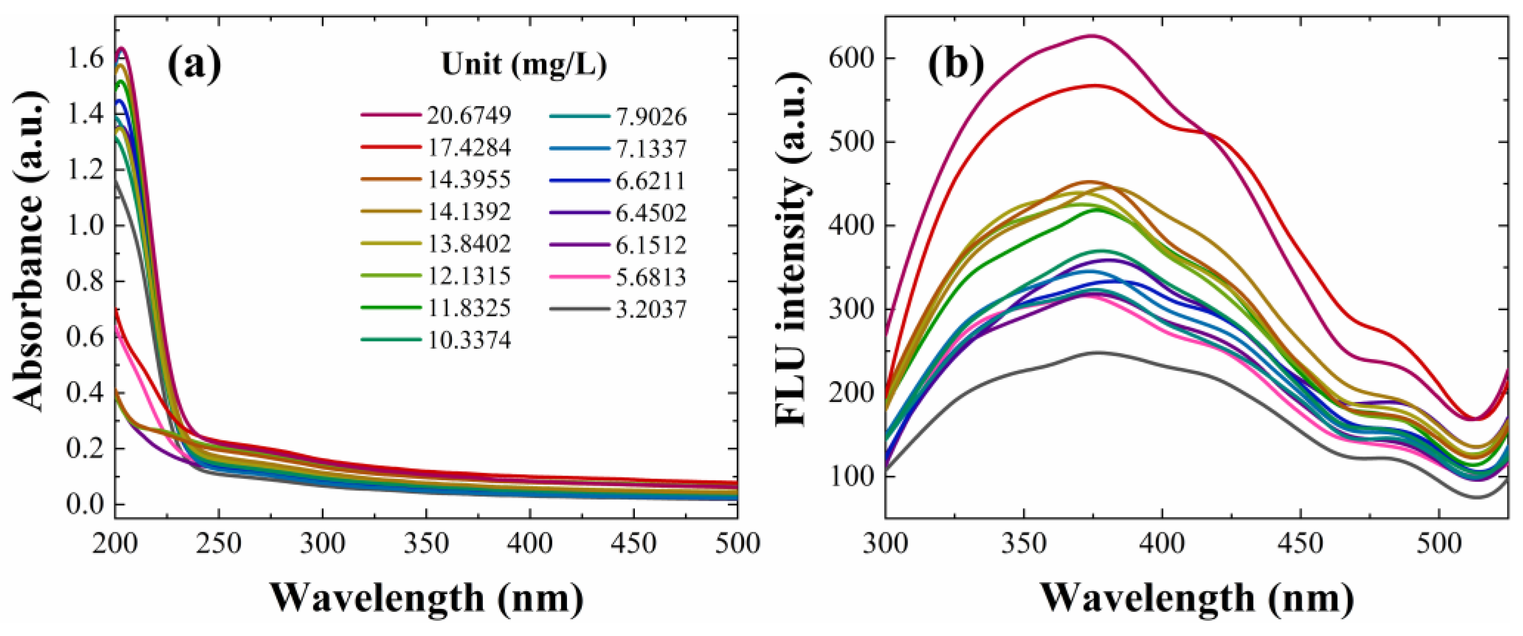
2.2. Spectra Acquisition

The measurement of the UV–vis spectrum was conducted using an American PerkinElmer Lambda 950 spectrophotometer and the usable wavelength range was from 175 to 3300 nm. The optical system has a SiO₂-coated holographic ruled grating with the highest wavelength accuracy of 0.08 nm. Before detecting the UV–vis absorbance of the solution, deionized water was used as a reference to eliminate the absorption of light by water. We measured the spectral absorbances of samples from 200 to 500 nm when the optical path was adjusted to 1 nm. Due to the complex composition of the actual water samples and the presence of noise interference during some tests, the collected spectral data may fluctuate and deviate from the baseline. Before modeling, we preprocessed the collected spectral data using Savitzky Golay (SG) filters. As this is a commonly used data smoothing method, the shape of the original spectrum will not change after SG processing, but the signal-to-noise ratio of the spectrum can be significantly improved.

As shown in Figure 1a, due to the presence of unsaturated structural organic pollutants (conjugated systems containing aromatic hydrocarbons, double bonds, and carbonyl groups) and some inorganic ions in water, we can observe that samples have significant absorption peaks at around 210 nm. For the FLU experiments, we used a USA PerkinElmer (Waltham, MA, USA) LS 55 fluorescence spectrophotometer. The variable range of the excitation light path slit (spectral passband) is from 2.5 to 15 nm, and the variable range of the emission light path is from 2.5 to 20 nm. We set the excitation wavelength of the FLU spectrometer to 285 nm and measured the emission spectra of the samples. As shown in Figure 1b, the mapping relationship between the FLU intensity and the content of organic matter has been established. The water samples have obvious emission peaks in the wavelength range of 300 to 500 nm. Compared with UV–vis spectroscopy, FLU spectroscopy has a wider effective range of spectral information. Even at COD = 3.2 mg/L, the FLU spectra can be well characterized.

3. Model Algorithm

Considering the insufficient number of sampled water bodies, we use the LSSVM algorithm to model the spectral data. To reduce the redundancy of the spectral data, we use feature selection methods to achieve data dimensionality reduction, including the SPA and CARS algorithms. The SPA algorithm is a forward iterative search method, which selects the most important wavelength point in the spectral information through projection in the vector space [28,29]. The CARS algorithm is a feature variable selection method that combines the Monte Carlo and PLS model regression coefficients. By using the subset with the lowest root-square error of cross-validation (RMSECV) value, the best combination of variables can be efficiently found. The LSSVM algorithm replaces the inequality constraints in SVM with equality constraints, which can use fewer sample variables for model learning in high-dimensional space and solve the problem of the insufficient number of samples [30,31].

Information fusion is the process of cognition, synthesis, and judgment of various data [32]. According to different fusion methods and levels, information fusion can be divided into three types: data-level fusion, feature-level fusion, and decision-level fusion. As a result of directly processing the original data, although data-level fusion has less information loss, the corresponding model is computationally intensive and restrictive. Feature-level data fusion extracts and processes the original data before fusion to form a new spectral matrix, thereby reducing the amount of calculation and increasing the proportion of information. Based on model fusion, decision-level data fusion makes a comprehensive decision on the final results through a voting mechanism. This approach increases the fault tolerance of the model while improving the anti-interference ability, which can be expressed as

$$y_{pred}=k_1{y}_{modelA}+k_2{y}_{modelB}$$

(1)

where $y_{modelA}$ and $y_{modelB}$ are the predictive results of models A and B, respectively; $k_1$ and $k_2$ are the weight coefficients of $y_{modelA}$ and $y_{modelB}$ determined by the voting mechanism; and $y_{pred}$ represents the final comprehensive decision result.

The technique for order preference by similarity to the ideal solution (TOPSIS) method is a comprehensive decision-making method [33]. The objective assignment of entropy weights is used to calculate the information entropy of the index. The relative change degree of index impact on the whole system determines its weight coefficient. At the same time, the optimal and inferior solutions among the finite solutions can be obtained in the normalized original data matrix. The distances between the evaluated subjects and the two solutions are calculated separately, which can be used as a basis to evaluate the grades of the samples.

The indicator matrix (assuming there exist m water quality samples and n concentration indicators) can be expressed as

$$X=\left(\begin{array}{ccc}{X}_{11}& \cdots & X_{1n}\\ ⋮& \ddots & ⋮\\ X_{m1}& \cdots & X_{mn}\end{array}\right)=\left\{X_{ij}\right\}$$

(2)

where $X_{ij}$ represents the jth concentration index of the corresponding ith sample. The large dispersion of $X_j$ means that the indicator plays a greater role in the overall evaluation. The entropy value $e_j$ and weight value $W_j$ of the jth index can be calculated with the following equations:

$$e_j=-\frac{1}{\ln m}{{\displaystyle \sum }}_i^m{P}_{ij}\ln P_{ij}$$

(3)

$$W_j=\frac{1-e_j}{{{\displaystyle \sum }}_{j=1}^n\left(1-e_j\right)}$$

(4)

where $P_{ij}$ indicates the proportion of the ith sample in the jth indicator and $1-e_j$ corresponds to the information redundancy value of each indicator. The value of $1-e_j$ is proportional to the amount of information it contains. According to the calculated weights $W_j$, the weighting matrix $X^{*}$ can be obtained by multiplying each sample. Finally, we can obtain the relative approximation $C_i$ to evaluate each indicator and the corresponding weights.

$$C_i=\frac{D_i^{-}}{\left(D_i^{+}+D_i^{-}\right)}$$

(5)

$D_i^{+}=\sqrt{{\displaystyle \sum }_j{\left(X_{ij}^{*}-X_j^{*+}\right)}^2}$ and $D_i^{-}=\sqrt{{\displaystyle \sum }_j{\left(X_{ij}^{*}-X_j^{*-}\right)}^2}$ indicate the optimal and inferior distances. $X_{ij}^{*+}$ and $X_{ij}^{*-}$ are the optimal and inferior solutions obtained from the weighting matrix $X^{*}$, respectively.

A random forest (RF) algorithm can rank the importance by analyzing the magnitude of the contribution made by each feature [34,35]. Variable importance measures (VIMs) can be expressed by the Gini index (GI). The $G{I}_q^{\left(i\right)}$ and $VI{M}_{jq}^{\left(Gini\right)\left(i\right)}$ indicate the Gini index and feature importance of the feature $x_j$ at the ith tree node q. Based on $G{I}_q^{\left(i\right)}$ and $VI{M}_{jq}^{\left(Gini\right)\left(i\right)}$, the importance of feature $x_j$ in the ith tree $VI{M}_j^{\left(Gini\right)\left(i\right)}$ can be obtained. $VI{M}_j^{\left(Gini\right)}$ is the sum of $x_j$ in decision trees, which can be expressed with $VI{M}_j^{\left(Gini\right)}={\displaystyle \sum }_{i=1}^{I}VI{M}_j^{\left(Gini\right)\left(i\right)}$. The final normalized importance score for each indicator can be expressed as

$$VI{M}_j^{\left(Gini\right)}=\frac{VI{M}_j^{\left(Gini\right)}}{{{\displaystyle \sum }}_{j^{\prime }=1}^{J}VI{M}_{j^{\prime }}^{\left(Gini\right)}}$$

(6)

4. Results and Analysis

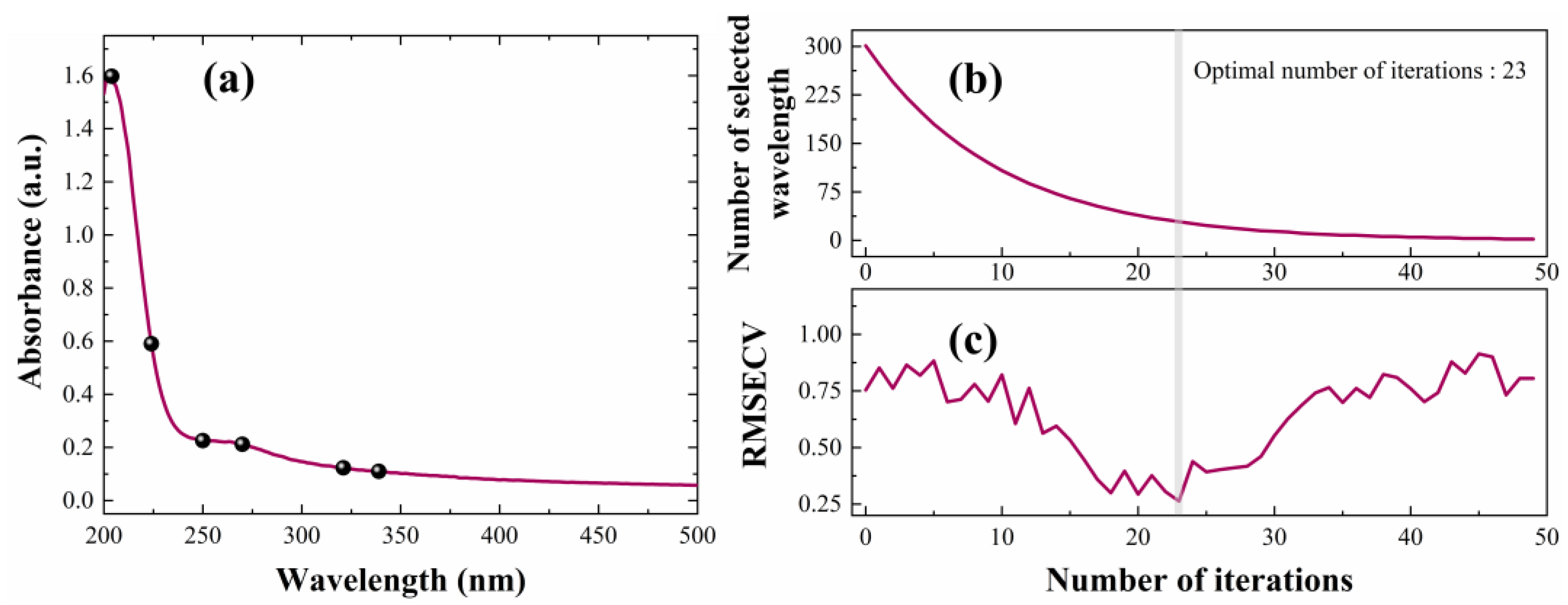
4.1. Spectral Feature Selection

As shown in Figure 1a, the UV–vis absorption of the water sample is mainly concentrated in the 200 nm to 300 nm band [36]. We note that the absorbance curves after 300 nm overlap without significant spectral features. To reduce the redundant information, we use the SPA and CARS algorithms to select the feature wavelengths. Based on the SPA algorithm, the minimum RMSECV of 0.1502 can be obtained when the selected wavelength point is 6, which achieves the best result [37]. The selected wavelength points are shown in Figure 2a. For the CARS algorithm, the number of selected variables gradually reduces with the increased iterations, as shown in Figure 2b. However, the RMSECV value exhibits a non-monotonic trend that decreases first and then increases. The reduced RMSECV indicates that some useless information in spectral data has been eliminated first. Meanwhile, the increased values indicate that some important information may be lost during modeling. Based on the CARS algorithm, the RMSECV can reach a minimum value of 0.2631 when the number of iterations is 23, as shown in Figure 2c. During the feature-selection process, 29 wavelength points are selected.

Accordingly, we also use the SPA and CARS algorithms for the feature selection of the pre-processed FLU emission spectra. Based on the SPA, the minimum RMSECV of 0.3341 can be obtained when the selected wavelength point is 9, as shown in Figure 3a. From Figure 3b,c, RMSECV reaches the minimum value of 0.304 in 24 iterations based on the CARS algorithm. During the feature-selection process, 34 wavelength points are selected.

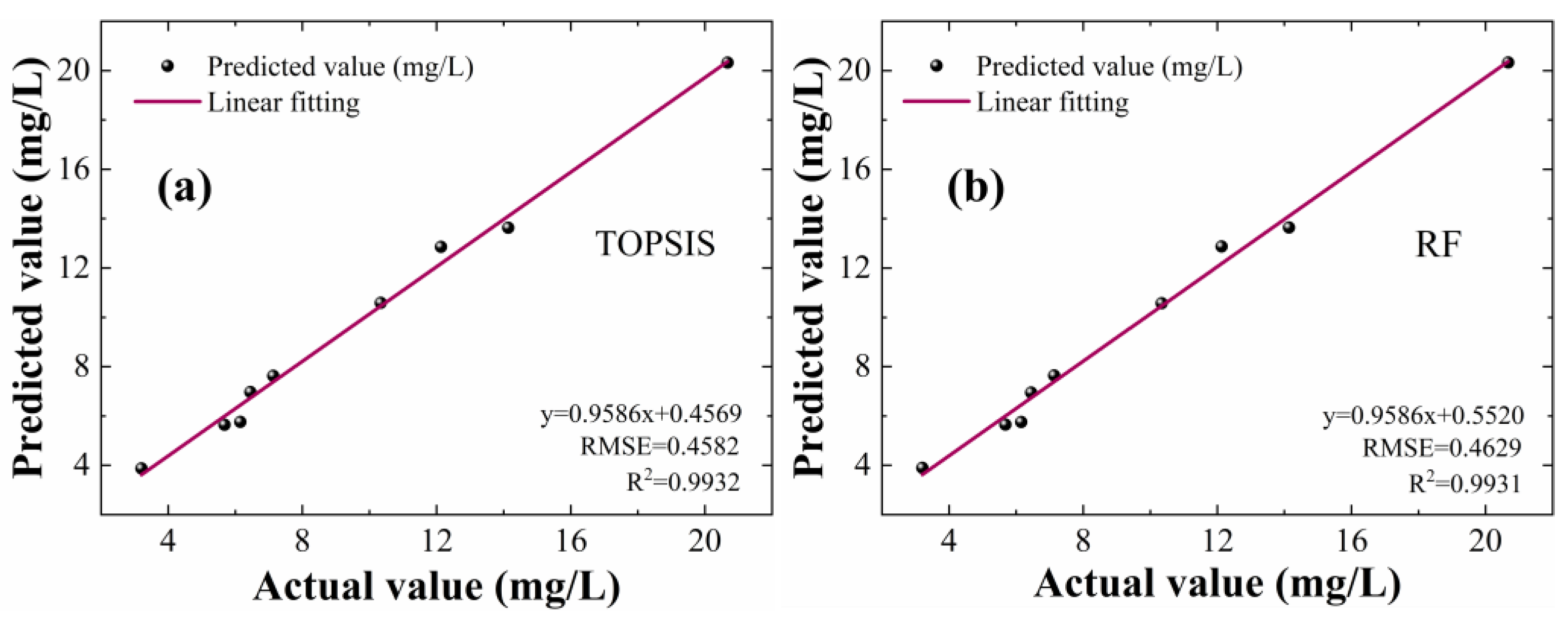
4.2. Analysis and Comparison of Modeling Results

Using the LSSVM method, we establish corresponding predictive models based on the feature selection of UV–vis and FLU spectral data for analysis and comparison. During the modeling process, 80% of the samples are assigned to the training set and the remaining 20% are assigned to the predictive set. In the UV–vis single-spectrum model, the values of $R^2$ and RMSE obtained by CARS feature selection are 0.9466 and 1.3698, respectively, while in the SPA model, they are 0.9318 and 2.2109. Correspondingly, in the FLU single-spectrum model, the $R^2$ and RMSE of the CARS model are 0.9680 and 1.2909, and those of the SPA model are 0.9068 and 2.3423. After feature selection, the predictive accuracies of the two single-spectrum models are still relatively low.

To avoid the limitations of the single-spectrum model in the analysis of complex water bodies, we combine UV–vis and FLU spectra through information fusion technology. Based on SPA and CARS feature selection, we de-quantified the two spectral datasets to construct new feature matrices [38,39]. After feature-level data fusion, the important information results contained in the UV–vis and FLU spectra are combined. We make a linear fit between the obtained predicted results and the real COD values, as shown in Figure 4a,b.

Compared with the single-spectrum model, the determination coefficient $R^2$ and RMSE of the models have been significantly improved after data fusion. For SPA feature selection, the $R^2$ and RMSE can reach 0.9754 and 0.9079, respectively. Correspondingly, the $R^2$ and RMSE are 0.9830 and 0.7886 with the CARS algorithm. By contrast, although they are all feature-level data fusions, the linear fitting effect based on the CARS algorithm is better than that of the SPA model. The data after feature selection removes most of the redundant information from the original data and reduces the data dimensionality. Feature-level data fusion effectively retains spectral data while removing interfering information, achieving better predictive results.

To further improve the predictive accuracy of the model, we optimize the two spectral models at the decision level. Based on the feature-level fusion models of CARS and SPA, we label the results as $y_{CARS}$ and $y_{SPA}$, respectively. As a comparison, we adopt the voting mechanism of the TOPSIS and RF algorithms for decision-level data fusion [40,41]. For the TOPSIS algorithm, we combine the entropy weight with the optimal and inferior distances of $D_i^{+}$ and $D_i^{-}$ to obtain the composite score and weight of each indicator. The final weight coefficients assigned to the CARS and SPA feature-selection-based fusion models are 0.5279 and 0.4721, respectively. Based on TOPSIS, the results of decision-level data fusion can be expressed as

$$y_{pred\left(TOPSIS\right)}=0.5279\times y_{CARS}+0.4721\times y_{SPA}$$

(7)

For the RF algorithm, we can evaluate each indicator by calculating the Gini index of each feature to determine the corresponding weight [42]. The final weight coefficients assigned to the CARS and SPA feature-selection-based fusion models are 0.5031 and 0.4969, respectively. Based on RF, the results of decision-level data fusion can be expressed as

$$y_{pred\left(RF\right)}=0.5031\times y_{CARS}+0.4969\times y_{SPA}$$

(8)

The final predictive results obtained by the two voting mechanisms are shown in Figure 5a,b. It is worth noting that after data fusion at the decision level, the predictive accuracy and stability achieve an excellent performance during the fitting process. The determination coefficient $R^2$ between the predicted value and the real value can reach up to 0.99. At the same time, the RMSE of the model is reduced significantly. For example, the RMSE obtained from the TOPSIS voting mechanism is reduced to 0.4582, which is 41.9% lower than the corresponding feature-level data fusion model. After decision-level data fusion, we find that there is little difference between the predictive models of the two chosen voting mechanisms due to the significant improvement in accuracy. For better presentation, we list the predictive results of all models in

Table 2. Summary of the predictive results obtained by single-spectrum models, feature-level fusion models, and decision-level fusion models, respectively.

Model	UV–vis		FLU		Feature-Level Fusion		Decision-Level Fusion
	CARS	SPA	CARS	SPA	CARS	SPA	ENTROPY TOPSIS	RF
RMSE (mg/L)	1.3698	2.2109	1.2909	2.3423	0.7886	0.9079	0.4582	0.4629
R2	0.9466	0.9318	0.9680	0.9068	0.9830	0.9754	0.9932	0.9931

. Compared with the single-spectrum model, the accuracy of the model has been greatly improved after data fusion. During the feature selection process, the accuracy of the CARS algorithm is better than that of the SPA algorithm. Considering the accuracy and stability of the model, the decision-level data fusion model based on entropy weight TOPSIS achieves the best prediction performance, making it more valuable for predicting forest surface waters with relatively low COD values. To better demonstrate the results of our model, we make a comparison with the representative results mentioned in the introduction, including the UV–vis and FLU single-spectrum models. Combined with the CNN model, Xin Liu’s group realized the optimization of the COD prediction model (R² = 0.9991, RMSE = 3.8745) using UV–vis spectra [7]. Compared with them, the RMSE value of our model is reduced by 88.17%. Weihong Bi’s group used feature-level data fusion to detect COD in FLU spectra at excitation wavelengths of 265, 290, and 305 nm, which significantly improved the accuracy of detection (R² = 0.9982, RMSE = 0.5342) [8]. Compared with their single-FLU-spectrum model, the RMSE value of our multispectral model is reduced by 14.2%. The introduction of multispectral data further improves the anti-interference ability of the model. Considering the differences in the COD concentration range of actual water bodies, the water samples in this paper mainly come from forest water bodies with low COD concentrations. To further improve the generalization ability of the model, more test samples and various environmental factors can be added for comprehensive consideration.

5. Conclusions

In summary, we have demonstrated COD prediction for real forest water samples based on UV–vis and FLU spectroscopy. Due to the large amounts of spectral information, high data dimensionality, and noise interference, the SPA and CARS algorithms are introduced in the feature-selection process. By comparison, the model selected based on CARS has higher accuracy, less error, and higher stability than the SPA model. However, the RMSE values of the two single-spectrum models both exceed 1, which cannot meet the accuracy requirements. Considering the deficiencies of the existing UV–vis and FLU spectrum models that cannot be well resolved by soft compensation, we use feature-level and decision-level data fusion methods to further optimize the predictive model. After feature-level fusion, the RMSE and $R^2$ values of the model can be optimized to 0.7886 mg/L and 0.9830. Accordingly, with the decision-level data fusion, the RMSE value has been further reduced to 0.4582 mg/L, which is 64.51% and 41.90% lower than those of the single-spectrum and feature-level fusion models, respectively. At the same time, $R^2$ is also increased to 0.9932. In forest water COD detection, the decision-level data fusion model based on two voting mechanisms greatly improves prediction stability and reliability of UV–vis and FLU spectroscopy. Our research lays the foundations for monitoring the pollution of water bodies around forest lands and assessing the impact of human activities on forest ecosystems. Thus, it makes it easier to take effective prediction and management measures to promote the sustainable development of forest protection.

References

1. Geerdink, R.B.; Sebastiaan van den Hurk, R.; Epema, O.J. Chemical Oxygen Demand: Historical Perspectives and Future Challenges. Anal. Chim. Acta 2017, 961, 1–11. [Google Scholar] [CrossRef] [PubMed]
2. Ma, J. Determination of Chemical Oxygen Demand in Aqueous Samples with Non-Electrochemical Methods. Trends Environ. Anal. Chem. 2017, 14, 37–43. [Google Scholar] [CrossRef]
3. Gandaseca, S.; Rosli, N.; Ngayop, J.; Arianto, C.I. Status of Water Quality Based on the Physico-Chemical Assessment on River Water at Wildlife Sanctuary Sibuti Mangrove Forest, Miri Sarawak. Am. J. Environ. Sci. 2011, 7, 269–275. [Google Scholar] [CrossRef] [Green Version]
4. Li, J.; Luo, G.; He, L.J.; Xu, J.; Lyu, J. Analytical Approaches for Determining Chemical Oxygen Demand in Water Bodies: A Review. Crit. Rev. Anal. Chem. 2018, 48, 47–65. [Google Scholar] [CrossRef] [PubMed]
5. Sagan, V.; Peterson, K.T.; Maimaitijiang, M.; Sidike, P.; Sloan, J.; Greeling, B.A.; Maalouf, S.; Adams, C. Monitoring Inland Water Quality Using Remote Sensing: Potential and Limitations of Spectral Indices, Bio-Optical Simulations, Machine Learning, and Cloud Computing. Earth-Sci. Rev. 2020, 205, 103187. [Google Scholar] [CrossRef]
6. Chen, J.; Liu, S.; Qi, X.; Yan, S.; Guo, Q. Study and Design on Chemical Oxygen Demand Measurement Based on Ultraviolet Absorption. Sens. Actuators B Chem. 2018, 254, 778–784. [Google Scholar] [CrossRef]
7. Jia, W.; Zhang, H.; Ma, J.; Liang, G.; Wang, J.; Liu, X. Study on the Predication Modeling of COD for Water Based on UV-VIS Spectroscopy and CNN Algorithm of Deep Learning. Spectrosc. Spectr. Anal. 2020, 40, 2981. [Google Scholar]
8. Kunpeng, Z.; Xufang, B.; Weihong, B. Detection of Chemical Oxygen Demand (COD) of Water Quality Based on Fluorescence Multi-Spectral Fusion. Spectrosc. Spectr. Anal. 2019, 39, 813–817. [Google Scholar]
9. Bengraïne, K.; Marhaba, T.F. Predicting Organic Loading in Natural Water Using Spectral Fluorescent Signatures. J. Hazard. Mater. 2004, 108, 207–211. [Google Scholar] [CrossRef]
10. An, H.; Zhai, C.; Zhang, F.; Ma, Q.; Sun, J.; Tang, Y.; Wang, W. Quantitative Analysis of Chinese Steamed Bread Staling Using NIR, MIR, and Raman Spectral Data Fusion. Food Chem. 2023, 405, 134821. [Google Scholar] [CrossRef]
11. Lin, H.; Lin, J.; Wang, F. An Innovative Machine Learning Model for Supply Chain Management. J. Innov. Knowl. 2022, 7, 100276. [Google Scholar] [CrossRef]
12. Jing, Z.L.; Pan, H.; Qin, Y.Y. Current Progress of Information Fusion in China. Chin. Sci. Bull. 2013, 58, 4533–4540. [Google Scholar] [CrossRef]
13. Ruser, H.; Leon, F.P. Informationsfusion—Eine Übersicht. Tech. Mess. 2007, 74, 93–102. [Google Scholar] [CrossRef]
14. Lin, J.; Bai, D.; Xu, R.; Lin, H. TSBA-YOLO: An Improved Tea Diseases Detection Model Based on Attention Mechanisms and Feature Fusion. Forests 2023, 14, 619. [Google Scholar] [CrossRef]
15. Khaleghi, B.; Khamis, A.; Karray, F.O.; Razavi, S.N. Multisensor Data Fusion: A Review of the State-of-the-Art. Inf. Fusion 2013, 14, 28–44. [Google Scholar] [CrossRef]
16. Xiao, F. Multi-Sensor Data Fusion Based on the Belief Divergence Measure of Evidences and the Belief Entropy. Inf. Fusion 2019, 46, 23–32. [Google Scholar] [CrossRef]
17. Diez-Olivan, A.; Del Ser, J.; Galar, D.; Sierra, B. Data Fusion and Machine Learning for Industrial Prognosis: Trends and Perspectives towards Industry 4.0. Inf. Fusion 2019, 50, 92–111. [Google Scholar] [CrossRef]
18. Maimaitijiang, M.; Sagan, V.; Sidike, P.; Hartling, S.; Esposito, F.; Fritschi, F.B. Soybean Yield Prediction from UAV Using Multimodal Data Fusion and Deep Learning. Remote Sens. Environ. 2020, 237, 111599. [Google Scholar] [CrossRef]
19. Hua, M.; Xu, Z. Physical Random Access Signal Design for 5G Mobile Satellite Communication Systems. Phys. Commun. 2022, 55, 101908. [Google Scholar] [CrossRef]
20. Hua, M.; Zhang, T. Random Access Sequence Set Design in Wireless Cellular Communication Networks. Phys. Commun. 2023, 56, 101953. [Google Scholar] [CrossRef]
21. Yang, X.; Li, Y.; Wang, L.; Li, L.; Guo, L.; Yang, M.; Huang, F.; Zhao, H. Determination of 10-HDA in Royal Jelly by ATR-FTMIR and NIR Spectral Combining with Data Fusion Strategy. Optik 2020, 203, 164052. [Google Scholar] [CrossRef]
22. Li, Y.; Huang, Y.; Xia, J.; Xiong, Y.; Min, S. Quantitative Analysis of Honey Adulteration by Spectrum Analysis Combined with Several High-Level Data Fusion Strategies. Vib. Spectrosc. 2020, 108, 103060. [Google Scholar] [CrossRef]
23. Wang, L.; Meng, J.; Huang, R.; Zhu, H.; Peng, K. Incremental Feature Weighting for Fuzzy Feature Selection. Fuzzy Sets Syst. 2019, 368, 1–19. [Google Scholar] [CrossRef]
24. Hu, X.; Zhou, P.; Li, P.; Wang, J.; Wu, X. A Survey on Online Feature Selection with Streaming Features. Front. Comput. Sci. 2018, 12, 479–493. [Google Scholar] [CrossRef]
25. Lin, H.; Tang, C. Analysis and Optimization of Urban Public Transport Lines Based on Multiobjective Adaptive Particle Swarm Optimization. IEEE Trans. Intell. Transp. Syst. 2021, 23, 16786–16798. [Google Scholar] [CrossRef]
26. Lin, H.; Tang, C. Intelligent Bus Operation Optimization by Integrating Cases and Data Driven Based on Business Chain and Enhanced Quantum Genetic Algorithm. IEEE Trans. Intell. Transp. Syst. 2022, 23, 9869–9882. [Google Scholar] [CrossRef]
27. Lin, H.; Han, Y.; Cai, W.; Jin, B. Traffic Signal Optimization Based on Fuzzy Control and Differential Evolution Algorithm. IEEE Trans. Intell. Transp. Syst. 2022, 1–12. [Google Scholar] [CrossRef]
28. Wu, D.; Nie, P.; He, Y.; Wang, Z.; Wu, H. Spectral Multivariable Selection and Calibration in Visible-Shortwave near-Infrared Spectroscopy for Non-Destructive Protein Assessment of Spirulina Microalga Powder. Int. J. Food Prop. 2013, 16, 1002–1015. [Google Scholar] [CrossRef]
29. Tang, R.; Chen, X.; Li, C. Detection of Nitrogen Content in Rubber Leaves Using Near-Infrared (NIR) Spectroscopy with Correlation-Based Successive Projections Algorithm (SPA). Appl. Spectrosc. 2018, 72, 740–749. [Google Scholar] [CrossRef]
30. Wang, Z.; Niu, Y. Regional Electricity Consumption Based on Least Squares Support Vector Machine. In Proceedings of the Fifth International Conference on Machine Vision (ICMV 2012): Algorithms, Pattern Recognition, and Basic Technologies, Wuhan, China, 20–21 April 2012; Volume 8784, p. 87840C. [Google Scholar] [CrossRef]
31. Liu, Y.; Zhou, S.; Liu, W.; Yang, X.; Luo, J. Least-Squares Support Vector Machine and Successive Projection Algorithm for Quantitative Analysis of Cotton-Polyester Textile by near Infrared Spectroscopy. J. Near Infrared Spectrosc. 2018, 26, 34–43. [Google Scholar] [CrossRef] [Green Version]
32. Bleiholder, J.; Naumann, F. Data Fusion. ACM Comput. Surv. 2009, 41, 1–41. [Google Scholar] [CrossRef]
33. Meng, Q.; Zhang, C.; Song, T.; Li, N. The Application of the Improved TOPSIS Method in Bid Evaluation of Highway Construction. Appl. Mech. Mater. 2012, 178–181, 1365–1368. [Google Scholar]
34. Speiser, J.L.; Miller, M.E.; Tooze, J.; Ip, E. A Comparison of Random Forest Variable Selection Methods for Classification Prediction Modeling. Expert Syst. Appl. 2019, 134, 93–101. [Google Scholar] [CrossRef] [PubMed]
35. Chen, X.; Ishwaran, H. Random Forests for Genomic Data Analysis. Genomics 2012, 99, 323–329. [Google Scholar] [CrossRef] [Green Version]
36. Charef, A.; Ghauch, A.; Baussand, P.; Martin-Bouyer, M. Water Quality Monitoring Using a Smart Sensing System. Meas. J. Int. Meas. Confed. 2000, 28, 219–224. [Google Scholar] [CrossRef]
37. Huang, P.; Li, Y.; Yu, Q.; Wang, K.; Yin, H.; Hou, D.; Zhang, G. Classification of Organic Contaminants in Water Distribution Systems Developed by SPA and Multi-Classification SVM Using UV-Vis Spectroscopy. Spectrosc. Spectr. Anal. 2020, 40, 2267–2272. [Google Scholar]
38. Biancolillo, A.; Bucci, R.; Magrì, A.L.; Magrì, A.D.; Marini, F. Data-Fusion for Multiplatform Characterization of an Italian Craft Beer Aimed at Its Authentication. Anal. Chim. Acta 2014, 820, 23–31. [Google Scholar] [CrossRef]
39. Song, X.; Du, G.; Li, Q.; Tang, G.; Huang, Y. Rapid Spectral Analysis of Agro-Products Using an Optimal Strategy: Dynamic Backward Interval PLS–Competitive Adaptive Reweighted Sampling. Anal. Bioanal. Chem. 2020, 412, 2795–2804. [Google Scholar] [CrossRef]
40. Li, Y.; Zhang, J.Y.; Wang, Y.Z. FT-MIR and NIR Spectral Data Fusion: A Synergetic Strategy for the Geographical Traceability of Panax Notoginseng. Anal. Bioanal. Chem. 2018, 410, 91–103. [Google Scholar] [CrossRef]
41. Dhanalakshmi, C.S.; Madhu, P.; Karthick, A.; Mathew, M.; Vignesh Kumar, R. A Comprehensive MCDM-Based Approach Using TOPSIS and EDAS as an Auxiliary Tool for Pyrolysis Material Selection and Its Application. Biomass Convers. Biorefin. 2022, 12, 5845–5860. [Google Scholar] [CrossRef]
42. Menze, B.H.; Kelm, B.M.; Masuch, R.; Himmelreich, U.; Bachert, P.; Petrich, W.; Hamprecht, F.A. A Comparison of Random Forest and Its Gini Importance with Standard Chemometric Methods for the Feature Selection and Classification of Spectral Data. BMC Bioinform. 2009, 10, 213. [Google Scholar] [CrossRef] [PubMed] [Green Version]
Figure 1. Measured spectral data of actual water samples: (a) UV–vis absorbance and (b) FLU intensity varied with different concentrations of COD.
Forests 14 01361 g001
Figure 2. Results of feature selection for UV–vis spectra. (a) Selected feature wavelengths (spherical symbols) based on the SPA algorithm. (b) The number of selected wavelengths and (c) the RMSEV values varied with the iterations based on the CARS algorithm.
Forests 14 01361 g002
Figure 3. Results of feature selection for FLU spectra. (a) Selected feature wavelengths (spherical symbols) based on the SPA algorithm. (b) The number of selected wavelengths and (c) the RMSEV values varied with the iterations based on the CARS algorithm.
Forests 14 01361 g003
Figure 4. Fitting results between predicted values and actual values. (a) SPA and (b) CARS algorithm for feature-level data fusion.
Forests 14 01361 g004
Figure 5. Fitting results between predicted values and actual values. (a) TOPSIS and (b) RF voting mechanism for decision-level data fusion.
Forests 14 01361 g005