Article

Decision-Tree Application to Predict and Spatialize the Wood Productivity Probabilities of Eucalyptus Plantations

by
Clayton Alcarde Alvares
1,2,*,
Ítalo Ramos Cegatta
3,
Henrique Ferraço Scolforo
4 and
Reginaldo Gonçalves Mafia
5
1
Suzano SA Company, Lírio Correa Av., 1465, Limeira 13473-762, SP, Brazil
2
UNESP-FCA, Botucatu 18610-034, SP, Brazil
3
Suzano SA Company, São Paulo 01452-002, SP, Brazil
4
Suzano SA Company, Jacareí 12340-010, SP, Brazil
5
Suzano SA Company, Aracruz 29197-900, ES, Brazil
*
Author to whom correspondence should be addressed.
Forests 2023, 14(7), 1334; https://doi.org/10.3390/f14071334
Submission received: 19 April 2023 / Revised: 15 June 2023 / Accepted: 20 June 2023 / Published: 29 June 2023
(This article belongs to the Special Issue Machine Learning and Big Data Analytics in Forestry)

Abstract

:
Brazil is one of the world’s wood short-fiber producers, cultivating 7.5 million hectares of eucalypt trees. Foresters and resource managers often face difficulties in surveying reliable Eucalyptus productivity levels for the purpose of purchasing and prospecting lands. Spatial data science (DS) and machine learning (ML) provide powerful approaches to make the best use of the large datasets available today. Agriculture has made great use of these approaches, and in this paper, we explore how forestry can benefit as well. We hypothesized that both DS and ML techniques can be used to improve Eucalyptus productivity zoning based on multiple operational datasets of tree growth and environment. Based on more than 12,000 permanent forest inventory plots of commercial Eucalyptus plantations and the climate, soil, and altitude variables associated with them, a supervised ML approach was adjusted to model the forest plantation productivity. A multi-tuning of the decision-tree (DT) algorithm hyperparameters was prepared to yield 450 DT models, with a better one delivering an RMSE of 53.5 m3 ha−1, split in 35 terminal nodes, here interpreted as Eucalyptus productivity zones. The DT model showed an optimum performance index of 0.83, a coefficient of determination of 0.91, a root mean squared error of 12.3 m3 ha−1, and a mean absolute percentage error only of 3.1% in predicting the testing dataset throughout the study area. The DT rule set was interpreted in a user-friendly table and was prepared to classify any location within the study area in each one of the 35 productivity zones based on the required environment variables of the DT algorithm. The high quality of the model obtained made it possible to spatialize the DT rules, providing a reliable cartographic visualization of the probability levels of true Eucalyptus productivity for a huge region of forest-based industries in Brazil. These data-science techniques also provided a yield gap analysis using a very down-to-earth approach. We estimated a yield gap by an amount of 4.2 × 10⁷ m3, representing a few more than 113,000 ha, or 15% of the current forest base. This is the amount of avoided area expansion to accumulate the same wood stock in case the productivity is raised to the attainable level in each zone. This present study provided deeper analysis and reproducible tools to manage forest assets sustainably.

1. Introduction

Growing global demand for food and fiber [1], which added to the impacts of climate change [2], will require more efficient and resilient actions to consolidate the bioeconomy as a global economic system [3]. At the end of the day, the forest scientists and resource managers will provide more wood volume on less land.
Brazil is one of the world’s short-fiber wood baskets, home to some of the most productive and important multipurpose Eucalyptus plantations on the globe [4]. The country holds 7.5 million hectares of Eucalyptus plantations managed for the production of charcoal, panels, laminate flooring, paper, and mainly cellulose. The sector industries produced 21 million tons of pulp in 2020, seeing a strong increase of 90% in pulp exportation in the last 10 years worldwide (https://iba.org/eng, (accessed on 10 January 2022).
Historically, intensive research and development into forest growth in Southeastern Brazil outstandingly resulted in a fourfold increase in Eucalyptus productivity in the country from 1970 to 2015 [5]. However, most recently, the annual average Eucalyptus productivity growth rates dropped to zero when new forest expansions migrated to more climatically challenging regions of the country, which were still poorly understood ecophysiologically. New pests and issues related to variability and climate change have also exerted pressure to flatten the curve and fading productivity of Eucalyptus plantations in Brazil [6,7]. The impacts on Eucalyptus survival and productivity were well characterized during the dramatically long major droughts that struck Central–Southern Brazil between 2014 and 2015, between 2015 and 2016 in the Northern region, and between 2019 and 2021 again in Central–Southern Brazil, causing losses of hundreds of thousand hectares and a couple of billion dollars in forest assets [8,9,10].
Forest management mistakes in tropical regions generally result in larger yield gaps than in subtropical regions [11]. In-depth knowledge of production environments, their productivity levels, and the nature of their abiotic and biotic limitations are crucial points for the success of forest plantations in tropical regions. Most foresters know that the diverse physiographic and edaphoclimatic gradients found in tropical regions yield equally in diverse and complex production environments. Nonetheless, they often face difficulties in surveying their land’s reliable levels of productivity, basing their strategies on very site-specific models derived from purely empirical knowledge. Empirical models have their functionality in very specific situations where the rule set was created, as, for example, shown by Gava and Gonçalves [12]. Therefore, caution must be taken to avoid misunderstanding in any attempt of upscaling an empirical model.
The strategies used on productivity zoning should span multiple spatial scales and require a sound mechanistic understanding of the interactions between tree resource use dynamics over space and time. In Eucalyptus plantations, the use of ecophysiological and statistical models that incorporate climate variables such as rainfall or soil water deficit, adjusted with appropriate regionwide trials, are great examples to predict forest yield levels in target regions [13,14]. These studies have provided satisfactory results, but once based on experimental data generally scarcer, such approaches cannot perform distribution and probability modeling of the variable to be predicted.
Currently, most forest-based companies hold huge datasets of forest inventory and environmental monitoring with meteorological series and increasingly accurate soil and relief maps. However, in most cases, those tree growth and environment datasets are collected and used for purely operational purposes, despite foresters knowing such data remain latent for deeper applications to generate insights and other more powerful predictions. Hence, given the massive amount of data, available computational power, and balanced empirical and scientific knowledge, an opportunity arises to use spatial data-science (DS) and machine-learning (ML) concepts to improve the Eucalyptus productivity zoning.
DS is an interdisciplinary field that uses data collection, data curation, extraction, cleaning, analysis, model building, result visualization, and communication to abstract information and insights from large datasets [15]. ML refers to a set of available techniques in the toolbox of data scientists to produce predictions. ML is grouped into three categories, which include supervised, unsupervised, and reinforcement learning. Decision tree (DT) is a popular supervised classification that offers support in decision making, and it defines the logical structure, associated uncertainties, and constructive results of the decisions [15]. DT is a multifaceted machine-learning algorithm known as a glass-box model. After the DT model has determined the patterns in the training dataset, even readers with little or no machine-learning experience, after a brief explanation, might exactly and intuitively see what decisions will be made for a dataset that we want to predict. When it comes to ML, it is crucial to carefully weigh the trade off between estimation power and model interpretation. The DT algorithm excels at providing simple and straightforward results and interpretation models, showcased via elegant decision trees [16]. However, other ML methods that have a strong predictive ability often face challenges in terms of interpretation, reproducibility, and sharing capabilities [17,18,19].
In the tide of the digital world we live in today, there are many IT technicians working in large forest companies supporting digitizing processes and building big data. Nevertheless, they often take on roles beyond their professional skills, generally with a background in the basic sciences, and they rarely wet their feet in the field. Machine-learning algorithms used in forest ecology and management are prone to misinterpretation, which requires application with great caution. To avoid these interpretation problems, data scientists and foresters should go through the careful discovery phase. This includes the finding of relevant data, their formats from numerous sources to accomplish basic necessities, priorities, and objectives of the task, and also the major ecophysiological key cause–effect relationships involved in the studied case.
In a survey of machine-learning techniques for climate-based crop yield prediction, Elavarasan et al. [20] compared some existing supervised and unsupervised machine-learning models, and they concluded DT approach was faster and more precise, providing easily interpretable rules and assisting in identifying the significant fields. Pant et al. [21] made a comparison appraisal with a couple of machine-learning models to make maize, potatoes, rice, and wheat yield predictions and found that the DT regression resulted in the best accuracy for crop predictions compared to other algorithms, which linked to its reproducibility making the DT algorithm very powerful for solving problems in many applications on cash crops. Furthermore, the selection of predictor variables is another key point of a successful machine-learning implementation. Variables that are both strong predictors to target variables and simple to obtain or understand should be used. For example, for Eucalyptus productivity zoning, predictor variables such as temperature, rainfall, soil type, and altitude should be considered. Indeed, these major predictor variables fully converge with a literature review that showed these environmental features were the most applied in machine learning for crop yield prediction worldwide [22].
In the last 4 years, machine-learning usage for farm risk management has tripled [23]. Agriculture has made great use of these approaches [24], and in this paper, we explore how forestry can benefit as well. Numerous recent studies have employed various machine-learning techniques to assess the productivity of planted forests [25,26,27,28,29]. However, a notable limitation across these studies is the lack of comprehensive exploration regarding the tools utilized, deeper data visualizations, and the production of applicable and reproducible results and conclusions for end users. Furthermore, some of these studies have neglected multicollinearity in modeling analyses. This gap in the literature leaves a significant opportunity for further research and investigation to address these shortcomings and provide comprehensive and actionable insights for stakeholders in the field of planted forest productivity evaluation.
Therefore, our hypothesis suggests that the decision-tree approach can be utilized to enhance Eucalyptus productivity zoning by generating results that are transparent, reproducible, and based on multiple sets of operational tree growth data and environmental factors. The integration of decision-tree modeling allows for a more interpretable and explainable approach, shedding light on the key factors influencing Eucalyptus productivity. Additionally, this methodology facilitates the replication of results and fosters greater confidence in the zoning outcomes. Considering that, the objectives of this paper were fourfold: (1) to implement the data science and its components as discovery, data preparation, model building, model planning, model evaluation, result visualization, and communication on huge operational forest datasets; (2) to implement and assess a broad multi-tuning DT modeling approach to multiple datasets of tree growth and environment; (3) to perform zoning geographically explicit of the Eucalyptus productivity based on the adjusted DT model; (4) to determinate the Eucalyptus yield gaps using a machine-learning approach on a region-wide scale.

2. Materials and Methods
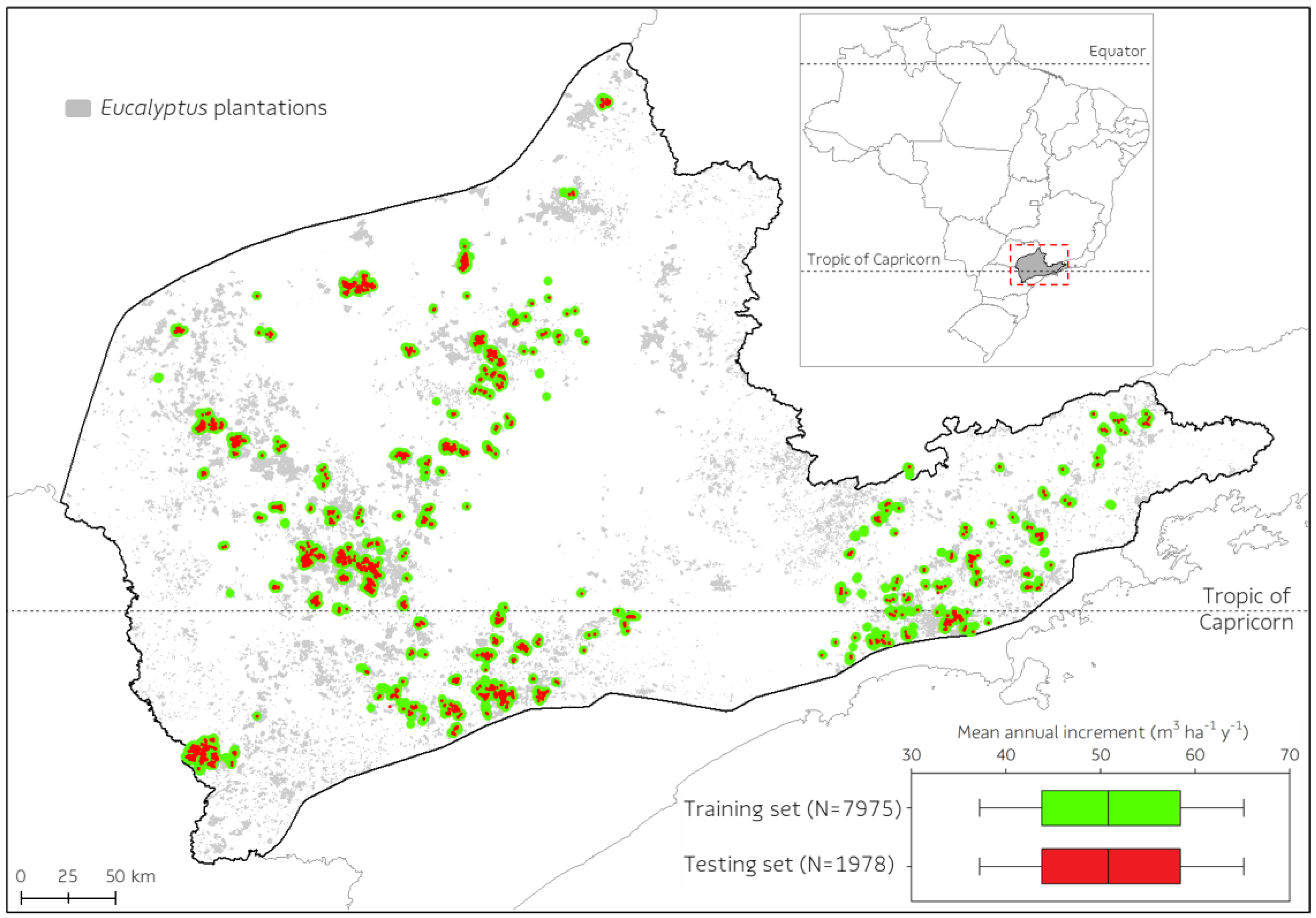
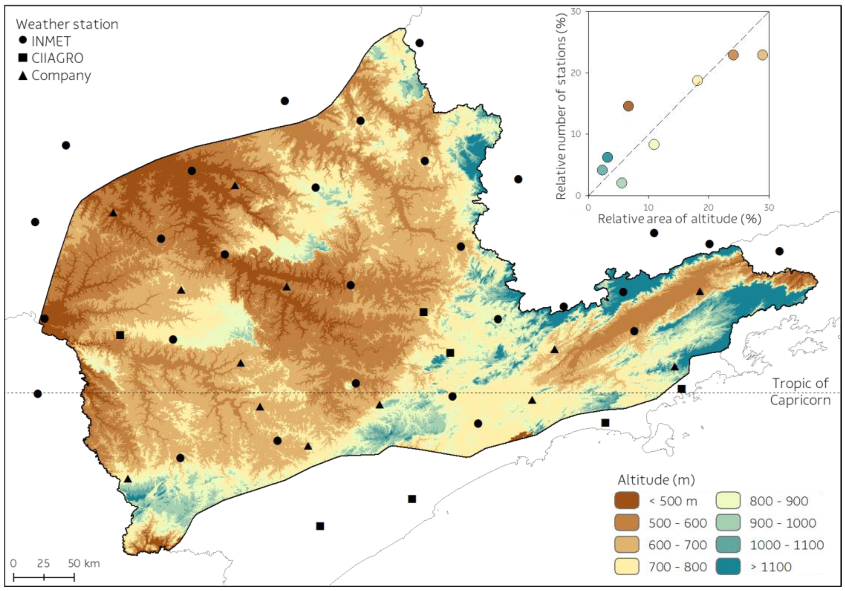
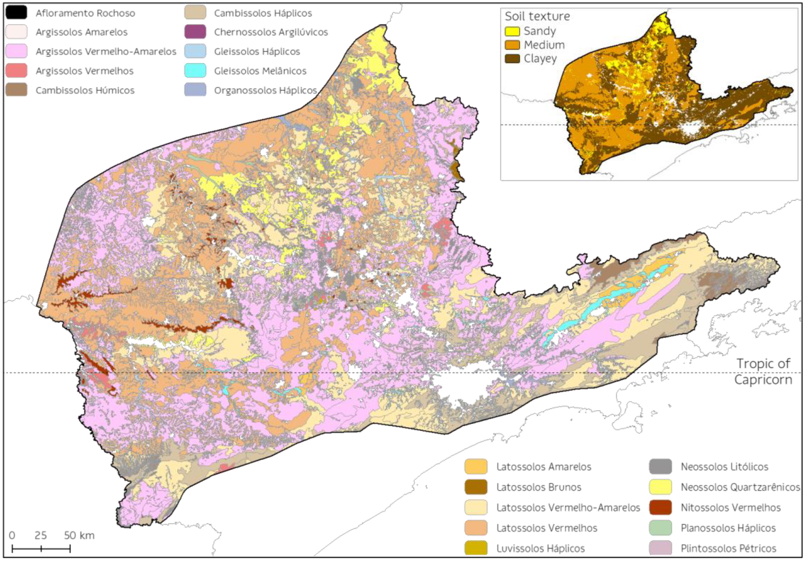
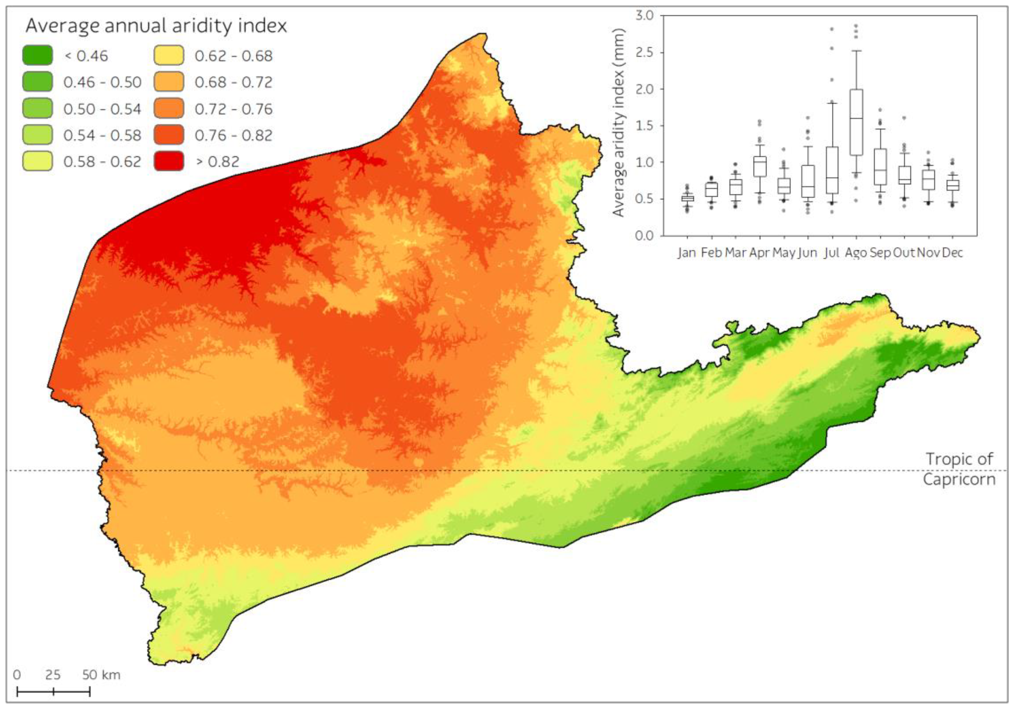
2.1. Study Area

The study area consists of approximately 11.4 million hectares located in Southeastern Brazil, covering nearly 46% of the State of São Paulo (Figure 1). According to the Spatial Database of Planted Trees [30], the State of São Paulo had in 2013/2014 approximately 823,619 hectares of Eucalyptus plantations belonging to companies in the pulp and paper, fiberboard, and wood panel industries, small growers, and participants in outgrower schemes and in state-owned forests. Of this total area, almost 95% of the Eucalyptus plantations (781,654 ha) were within the study area (Figure 1), i.e., the other 5% (41,965 ha) are well sparsely distributed in the 54% of the midwestern region of the state.
Covering different production environments and a large latitudinal gradient, the study area shows both tropical and subtropical features. Average annual temperature varies from 14 to 23 °C (on higher mountains, above 2000 m, average annual temperature can be as low as 14 °C), rainfall ranging 1200 to 2000 mm year−1, and the frost days hits are frequent in the southern part are main climatological traits of study area [31,32].
The study area has complex relief, with altitude ranging from 400 to 1500 m above mean sea level and a relevant geological diversity with parent sedimentary (sandstone, claystone, and siltstone), metamorphic (phyllites, shales, gneiss) and igneous (diabase and basalt) materials, resulting in large range of deep and shallow tropical soils distributed across the study area on erratic way on part regions [33,34,35].
Such geographic distribution of Eucalyptus plantations shows that the study area is one of the most traditional forest regions in the country with almost 100 years of experience in Eucalyptus silviculture [6,36] because it is one of the most favorable in world for silvicultural success due to its high suitability for dozens of Eucalyptus species [37].

2.2. Forest Datasets

Approximately 12,000 permanent forest inventory plots of commercial Eucalyptus plantations of the Suzano SA company (www.suzano.com.br/en, (accessed on 15 June 2023) at harvest time between 2013 and 2016 (with planting year between 2008 and 2011) were available for this study. Circular permanent inventory plots had an area of 400 m2 and were systematically distributed with a density of one plot per ten hectares. During field measurements, diameter at breast height (DBH, 1.3 m above the ground) of all trees, total height of the central ten trees, and the total height of the four largest trees in terms of DBH (defining dominant trees) were surveyed in the inventory plot. The mean height of these dominant trees defined the dominant height of the plot. Dominant height, basal area, and age on the inventory date were then used in local volume equations to estimate the total wood volume with bark for each plot. A total of 9953 forest inventory plots composed of 517,000 live trees (by a total of 528,000 trees) were selected for this study after tree data consistency, which included filtering them to have plots with (i) live trees between 800 and 1900 trees ha−1, (ii) age between 5.5 and 6.5 years (age class center of 6 years old) at harvest time, (iii) standard size plots, (iv) only first rotation forest (not coppice), (v) free pests and diseases plots, (vi) no record of plots faced strong weed competition and fire scars, and (vii) double checking its geographic location. Finally, a visual dispersion analysis of the permanent forest inventory plots database was required to ensure reliable analysis and modeling, with the final dataset clean-up dropping any strange relationship between basal area and total wood volume (Figure S1).
The forest inventory database was randomly divided into two datasets using a geographically weighted approach. The first, referred to as the training dataset, with 80% of all plots, was used in DT modeling exercise in order to build the productivity zones for planted Eucalyptus forests. Another group, called testing dataset, with 20% remaining plots (unseen data by the model), was used to perform the validation of the productivity zones output of the DT. The forest inventory dataset consisted of 70 pure or hybrid Eucalyptus clones of the species E. grandis, E. urophylla, E. smithii, and E. dunnii.

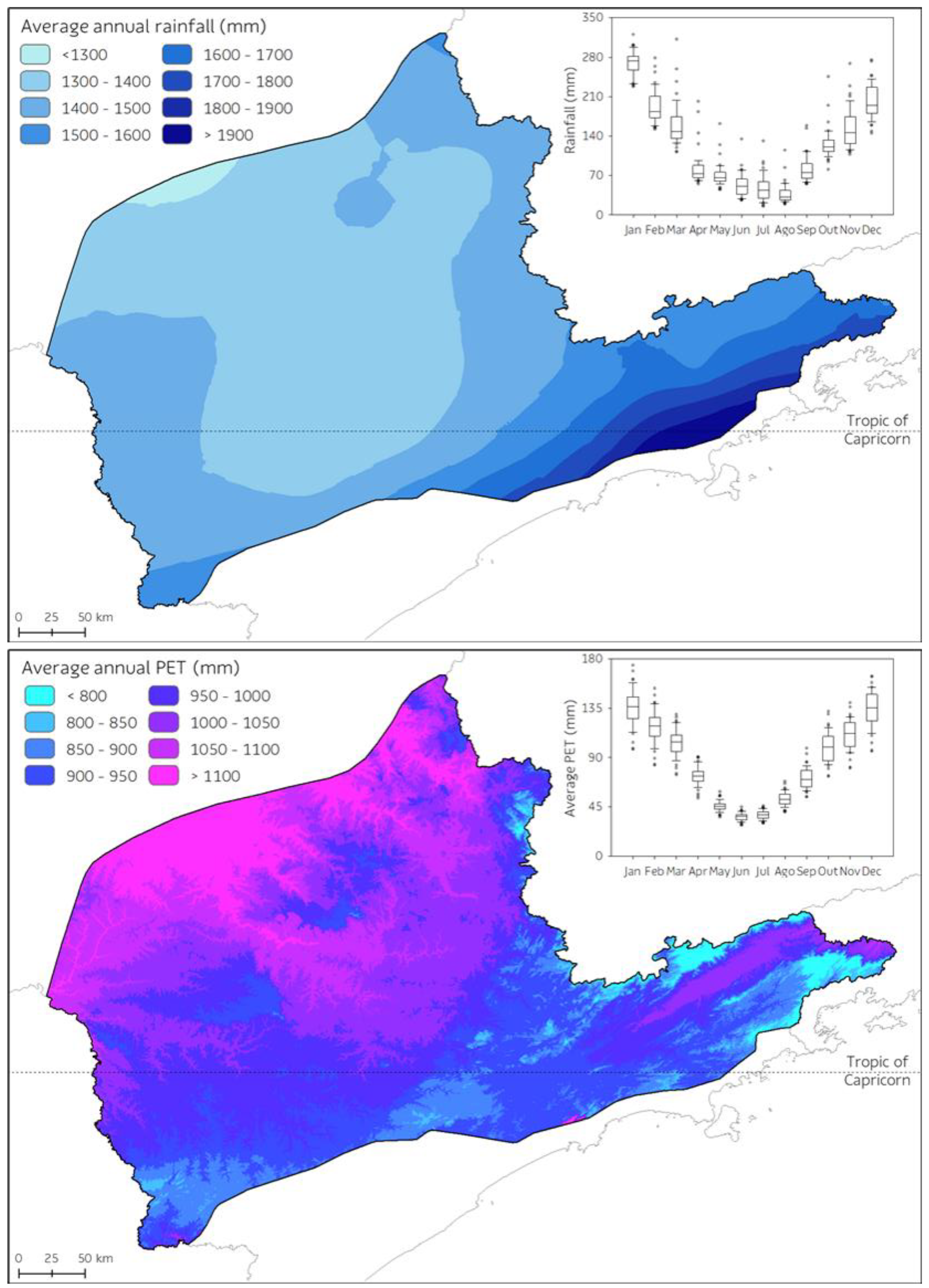
2.3. Environmental Datasets

For each forest inventory plot, information such as geographic location, altitude obtained in the field, average terrain slope, planting date, measurement date, genetic material, planting spacing, wood volume, rotation, soil order, and soil texture was provided.
Soil information of each plot is from company-owned detailed soil maps, surveyed at scale of 1:50,000 and elaborated by professional pedologists specialized in tropical soils. Those company soil maps cover only Eucalyptus stands. Well-developed and deep soils accounted for 57.3% of the plots, as the order Latossolos (L, Oxisols) with 43.1%, Argissolos (A, Ultisols) with 13.9%, and Nitossolos (T, Oxisols) with 0.4% remaining. On the other hand, less developed and/or shallow soils totaled for 42.5% of the plots, as Neossolos (N, Entisols) with 29.6%, and Cambissolos (C, Inceptisols) with 12.9% of them. Finally, 0.2% of the plots were classified as hydromorphic soil order Gleissolos (G, Entisols). Soil order names in Portuguese are according to the Brazilian Soil Classification System [38]. The symbol letter for soil order used on DT modeling and an approximate identification based on the USDA soil taxonomy are in parentheses [39].
Climatological data such as average annual temperature, average annual rainfall, average annual potential evapotranspiration, and aridity index were associated with each forest inventory plot. Meteorological data from a network of 48 automatic weather stations of the Brazilian National Institute of Meteorology (INMET, https://mapas.inmet.gov.br, (accessed on 15 May 2021)), Integrated Center of Agrometeorological Information of Campinas Institute of Agronomy (CIIAGRO/IAC, www.ciiagro.sp.gov.br/rede.html, (accessed on 15 May 2021)), and from the forest company, covering the entire study area, were used to develop the climatological database (Figure 2). We considered a climatic period of the last 26 years (1995 to 2020) to build maps of the monthly climatological normals for both air temperature and rainfall. The weather station datasets presented some data gaps in rainfall and air temperature records. Those missing data were filled with monthly gridded data published by Xavier et al. [40] at in spatial resolution of 0.25° and from NASA/POWER—NASA Langley Research Center POWER Project, which has recently been released at 0.5° × 0.5° grid cell [41].
Average annual rainfall dataset was analyzed according to geostatistical procedures proposed by Alvares et al. [31]. The omnidirectional experimental semivariogram for the annual rainfall data was prepared, whereas only 10 lag classes of equal intervals in a geometric field of 50% range dataset (latitude and longitude) was prepared. The experimental semivariogram was tested by adjusting them to the theoretical spherical, exponential, Gaussian, and linear models since they usually covered the general dispersion of environmental spatial events [42]. The best fit was based on the smallest reduced sum of squares and on the highest determination coefficient (R2). Using these structural parameters of the theoretical semivariogram extracted from experimental semivariogram, average annual rainfall map was composed with a geographic information system. A punctual ordinary kriging estimator was used for geostatistical interpolation. With these procedures, the annual rainfall map had a spatial resolution of 100 m.
The air temperature dataset was used to establish the relationship between the dependent (average air temperature) and independent (altitude, latitude, longitude, and their combinations) variables based on a general multivariate nonlinear regression model proposed by Alvares et al. [43] as follows (Equation (1)):
T i = a 0 + a 1 φ + a 2 λ + a 3 h + a 4 φ λ + a 5 φ h + a 6 λ h + a 7 φ 2 + a 8 λ 2 + a 9 h 2
where Ti is the average temperature, monthly (i = 1, 2, …, 12) or annual (i = 13); φ is latitude, in decimal degrees (negative in the southern hemisphere); λ is longitude, in decimal degrees (negative values for west of Greenwich meridian); h is altitude in meters; and a0 to a9 are the coefficients of the multivariate regression equation.
Using map algebra techniques [42,44], the results from the multivariate regression models for average monthly air temperature were converted into maps using the software ArcGIS [45], processing the independent variables as raster layer. The altitude layer, in meters, was obtained from the digital elevation model (DEM) provided by the Shuttle Radar Topography Mission (SRTM) [46] in its fourth version [47]. Subsequently, ArcGIS was used to build the DEM for stud area at 100 m resolution (Figure 2). Latitude and longitude layers were obtained in decimal degrees using the central coordinates of each pixel corresponding to the DEM. Using geoprocessing techniques [48,49,50], monthly air temperature models were programmed and run in ArcGIS.
After building the monthly temperature maps, we proceeded with the potential evapotranspiration calculations. Average annual potential evapotranspiration was estimated via the method of Thornthwaite [51]. Such method is very practical and easy to reproduce as it only requires the average monthly temperature observed as an input. The observed climatological normals are used to calculate Thornthwaite’s monthly and annual heat indices (Equations (3) and (4)). Latitude is used to calculate the photoperiod over the course of the year. Lastly, we must consider the number of days to adjust the potential evapotranspiration of each month (Equation (2)). After calculations, the monthly potential evapotranspiration maps were summed to obtain the annual potential evapotranspiration map.
PET i = 16 N 30 P 12 10 T i I a
I = i = 1 12 0.2 T i 2
a = 6.75 × 10 7 I 3 7.71 × 10 5 I 2 + 1.7912 × 10 2 I + 0.49239
where PETi is the estimated potential evapotranspiration of month i (mm); N is the number of days in month i; P is the average daily photoperiod of month i (hours); Ti is the average daily temperature of month i (°C); and a and I are the Thornthwaite’s heat indices, which depend on the average daily temperature of month i.
Based on annual potential evapotranspiration and annual rainfall maps, the aridity index was calculated (Equation (5)). Aridity index is an indicator for the degree of site dryness [52] and is used as the surrogate of water stress on Eucalyptus plantations [8,53]. After the spatializations of annual air temperature, annual rainfall, annual potential evapotranspiration, and aridity index, extractions of these data to populate the forest inventory plot datasets were performed.
Aridity   index = PET R
where PET is the estimated annual potential evapotranspiration (mm), and R is average annual rainfall (mm).

2.4. Decision-Tree Modeling

In order to guarantee the feasibility and reproducibility of the productivity zones for planted Eucalyptus forests by the foresters, small rural producers, forest beekeepers, participants interested in forest outgrower schemes, extension technicians, and researchers, a range of easily obtainable variables of climate, soil, and terrain were used to model and train the decision tree. One object of this study is to create a method that the end users can use in a straightforward way and apply the results of the productivity zoning model of planted Eucalyptus forests, thus maintaining the practicability of the system.
After the consistency and processing of tree growth and environmental data, each dataset was joined into a data frame composed of 9953 observations and 11 variables, which are as follows: forest inventory plot ID, latitude, longitude, training or testing dataset, genetic material, tree age, total wood volume with bark as the response variable; and the predictor variables as terrain altitude, soil order, soil texture, and average annual aridity index. However, some adaptations for DT algorithm were made as the smooth discretization of aridity index on the 0.015 scale and of ground altitude on the 20 m scale in order to have adequate aesthetics in the DT and easy interpretation of the thresholds of these predictive variables.
Based on the objectives of this study, the rpart package (Recursive Partitioning and Regression Trees [54]) and its routines for R software [55] were used to predict the productivity zones for planted Eucalyptus forests. The rpart’s main outcome is a recursive partitioning model displayed as a decision tree.
Before making our DT grow, we prepared a tuning using rpart hyperparameters that control aspects of the model fit. Basically, there are hyperparameters that control the growth and pruning of the DT as well as its complexity. Minbucket parameter is the minimum number of observations in any leaf (terminal) node. Minsplit parameter is the minimum number of observations that must exist in a node for a split to be attempted. Cost-complexity factor (cp parameter) is the metric that stops splits that are not deemed important enough to tree grow up and explain data.
A broad multi-tuning of the DT hyperparameters was planned. We wrote functions to control the hyperparameters during tuning approach that ranged as follows: minbucket parameter from 79 to 1000, by 100; minsplit parameter from 158 to 1000, by 100; and cp parameter tested the complexity measures of 0.01, 0.001, 0.0005, 0.0001, and 0.00001. Once DT modeling requires caution in terms of growth, pruning and trim, and tree complexity, we wrote functions to display the accuracy of each one DT outputted using the multi-tuning approach. The same function set also produced a visualization of ranging upper hyperparameters of decision-tree tuning process, supporting the better-chosen DT setup. Before departure of hyperparameter tuning modeling, we already assume a premise that minbucket parameters start at 79, i.e., the number of observations in the leaf node must be at least 1% of training dataset, ensuring an acceptable minimum forest and environmental representations of the data entries. Hence, we can notice minsplit parameter was set to start with 158 observations.
Once the DT model was defined and its best-fitting hyperparameters were set up, the next step was to assess the performance of the model making predictions of independent data (the 20% unseen data). For that, the testing set was used to validate the classification and regression model via the following relative errors indices: mean absolute error (MAE), root mean squared error (RMSE), and mean absolute percentage error (MAPE), respectively, as shown in Equations (6)–(8). The performance of the DT model was also tested using the Performance index “Pi” (Alvares et al. 2013b [43]), which is the product of the coefficient of correlation “r” (Equation (9)), which defines models’ precision, and the refined agreement index “dr” (Equation (10)) [56], which defines the models’ accuracy. The criteria for interpreting “Pi” (Equation (11)) include the following: Pi ≥ 0.75 as optimum performance; 0.6 ≤ Pi < 0.75 as very good performance; 0.45 ≤ Pi < 0.6 as good performance; 0.3 ≤ Pi < 0.45 as tolerable performance; 0.15 ≤ Pi < 0.3 as poor performance; 0 ≤ Pi < 0.15 as bad performance; Pi < 0 as very bad performance [43].
MAE = 1 N y i x i
RMSE = 1 N y i x i 2
MAPE = 100 N y i x i y i
r = x i x ¯ y i y ¯ x i x ¯ 2 y i y ¯ 2
dr = 1 y i x i c   y i y ¯ ,   when   y i x i   c   y i y ¯ c   y i y ¯ y i x i 1 ,   when   y i x i > c   y i y ¯
P i = r   ×   dr
where xi is the i-th observed value, yi is the i-th predicted value, N is the number of samples considered, x ¯ is mean of all observed values, y ¯ is mean of all predicted values, r is the Pearson’s correlation coefficient, dr is refined agreement index, c is 2, and P i is performance index.
Finally, after obtaining the final DT model, we wrote R functions that extracted the environmental predictor variable rules for each leaf node (Eucalyptus productivity zones) and put them in organized and straightforward way in an interpretive and illustrated table to be used by the end users.

2.5. Eucalyptus Forest Productivity Zoning

In this section, we deal with the geographic visualization of the DT outputs. Each DT leaf node was interpreted as a productivity zone for planted Eucalyptus forests, i.e., a production region’s average of Eucalyptus plantations productivity, observed at training dataset, is explained via the same environmental predictor variables and its thresholds.
We already reported the spatialized environmental predictor variables such as altitude and aridity index used to populate the training and testing datasets as independent data, as obtained in Section 2.3. Finally, the semi-detailed soil map of the State of São Paulo published by Rossi [57] was used to complete the required environmental information to apply the Eucalyptus forest productivity zoning outputted via DT. In total, this soil map has 247 soil mapping units, and it presented 20 soil classes (order and suborder) in the study area according to Figure 3. In order to use the soil map on DT modeling, each soil order found at Rossi [57] in study area, as already described in Section 2.3 for the soil information of the forest inventory plots, was coded as follows: A represents Argissolos; L represents Latossolos; N represents Neossolos; C represents Cambissolos; T represents Nitossolos; G represents Gleissolos; M represents Chernossolos. Likewise, the subsurface horizon soil texture identified by Rossi [57] received the code “a” for clayey texture (clay content > 35%), “m” for medium texture (15% < clay content < 35%), and “r” for sandy texture (15% < clay content). Soil order and soil texture vector maps were converted to raster in the spatial resolution of 100 m. Lastly, a prediction was made by transforming and spatializing each leaf node on productivity zones Eucalyptus for the whole study area based on DT rules and the predictor environmental variables.

3. Results and Discussion

3.1. Climate Modeling

The average annual rainfall dataset from 48 weather stations was analyzed according to the concepts of the regionalized variables theory [58]. Among the theoretical models tested, the spherical model best described the annual rainfall experimental semivariogram (nugget effect = 13,600; partial sill = 102,980; and range of spatial dependence = 7.3 degrees). The estimated residues were low and had a high coefficient of determination (R2 = 0.97). The average annual rainfall of the study area (Figure 4) has spatial variability similar to the current and official climatological normal map presented by Diniz et al. [59]. Average annual rainfall ranged from 1250 to 2050 mm, very similar to what was found in other studies [31,59].
All monthly and annual average air temperature multivariate regression models were significant (p < 0.001), and the independent variables obtained showed a significance of 5% (Table S1). Different from other studies [43,60], the combined predictor variables that used the square of altitude (h2) were significant at 5%, thus contributing to predicting the average air temperatures, both in monthly and annual time scales (Figure S2).
The average annual PET range (540–1220 mm) in the study area (Figure 4) was quite similar to that presented by Dias et al. [61]. Thereby, the ratio between annual PET and annual rainfall was applied to obtain the annual aridity index (Figure 5). The higher index identifies more arid environments. The average annual aridity index map showed the uplands and mountain regions, with altitudes above 900 m, mainly on the Serra do Mar range and the Mantiqueira region, where atmospheric water demands are very low, with an aridity index of less than 0.5. These upland regions have a water surplus of approximately 50% of the amount of annual rainfall, indicating high suitability for Eucalyptus growth [37]. Conversely, the aridity index exceeded 0.76 in most areas in the central–west region of the study area, denoting water stress throughout the year. Paraiba Valley (southeast of the study area) also has a high aridity index which certainly penalizes Eucalyptus productivity, as evidenced by many recent studies [5,8,14,62]. Our aridity index map ranges likewise to the one presented by Hubbard et al. [53]. These authors showed at tropical environments, the Eucalyptus trees grow according to soil water availability and that both high- and low-productivity Eucalyptus clones investigated transpired on average 60, 46, and 34% annual precipitation on dry (annual aridity index of 2.2), mesic (1.0), and wet (0.6) sites, respectively.

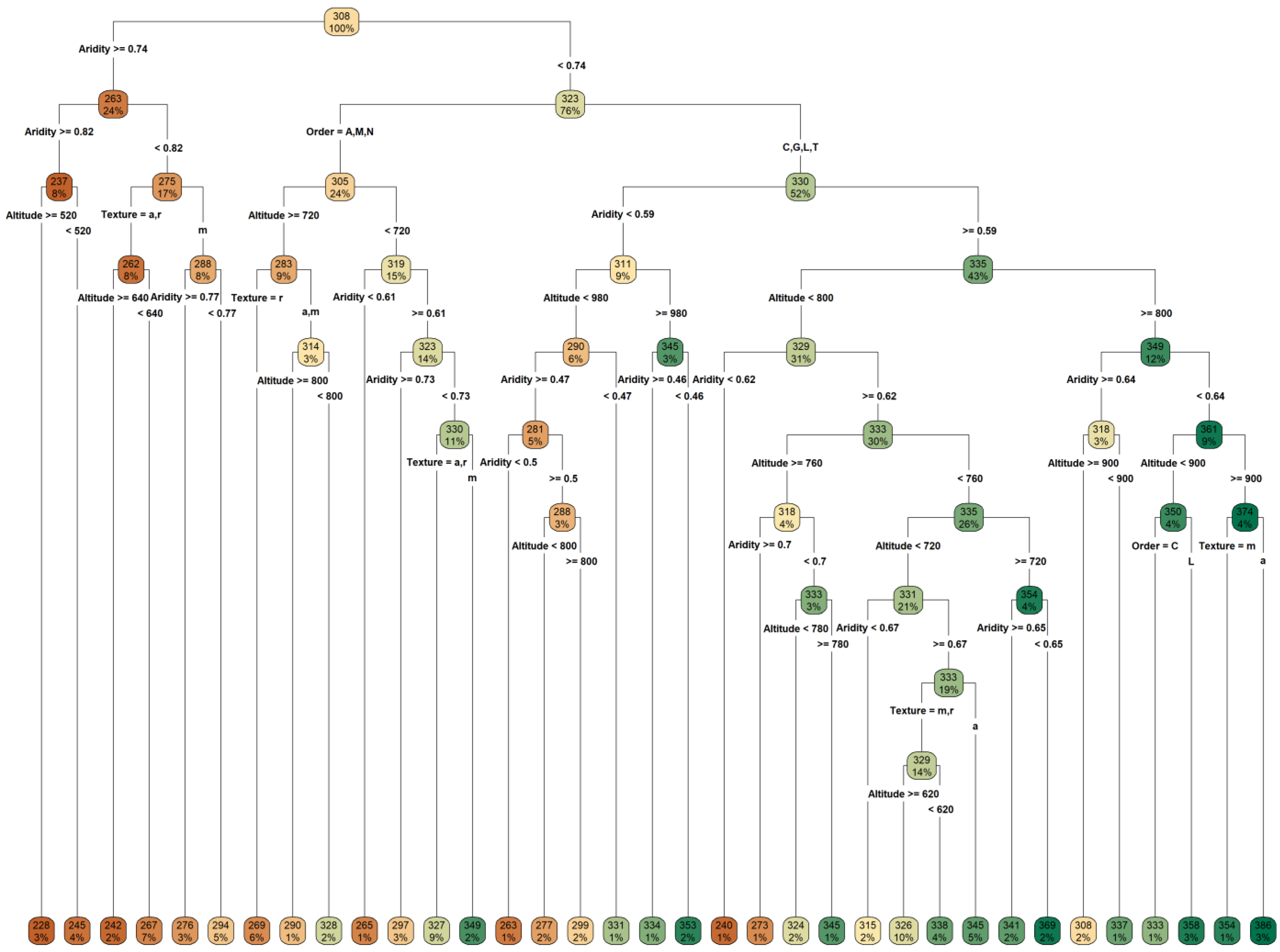
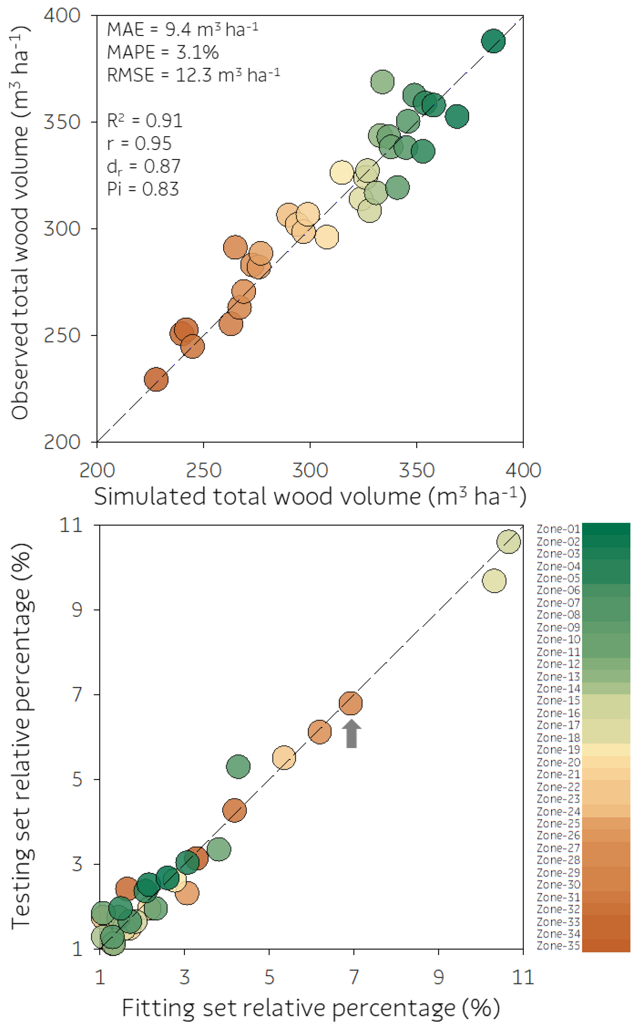
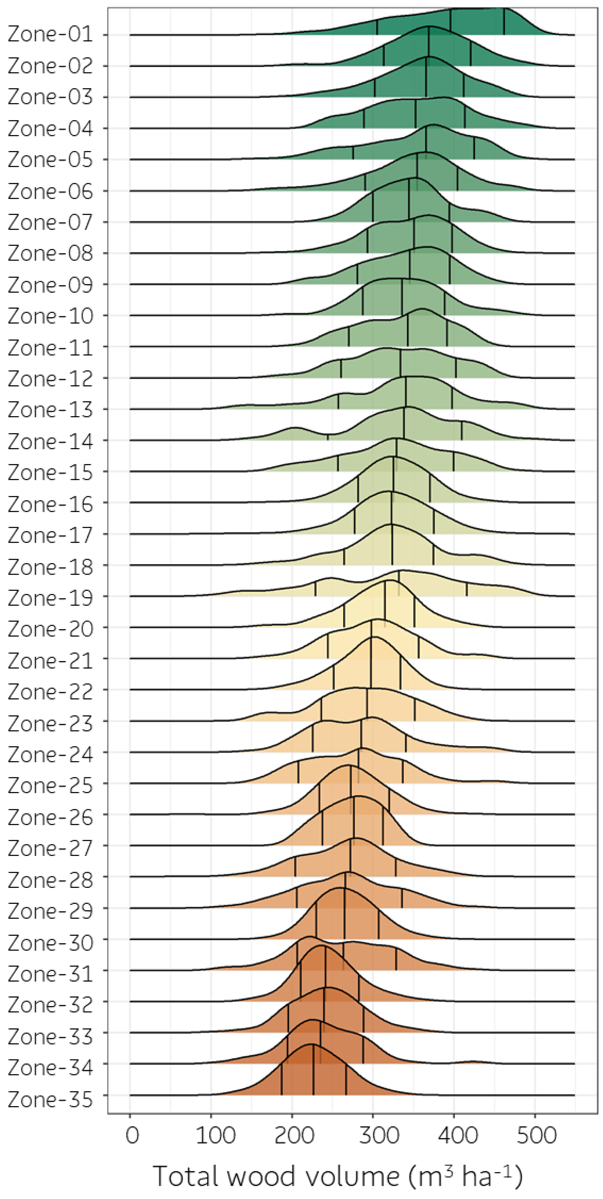
3.2. Decision-Tree Modeling

The hyperparameter tuning approach yielded 450 DT models, with RMSE ranging from 60.1 m3 ha−1 for the worst model to 53.3 m3 ha−1 for the best model. A scatter plot with all tuning modeling outputs allowed us to visualize a global exponential decay pattern between RMSE and the number of leaf nodes in each DT model, showing also that increasing the number of leaf nodes linearly reduces the RMSE for each one of the five cost-complexity factors applied (Figure S3). While Figure S3 provided an overview of tuning modeling, Figure S4 gave a zoom-in visualization of how all RMSE and the number of leaf nodes outputs are distributed between minsplit and minbucket hyperparameters for the cost-complexity factor = 0.0005. Among selecting the best DT by math tools like the minimum curve radius method, there is an important trade off with the empirical foresters’ knowledge. Therefore, the best and final DT was chosen based on those accuracy plot panels of the machine-learning algorithm modeling and on the practicality of the results and tools that were objectives of this study. Consequently, as expected and described previously, our premise considered that all leaf nodes must have at least 1% of the training dataset revealed via combining empirical and computational approaches because the better DT setup selected has the following hyperparameters: minbucket = 79, minsplit = 158, and cp = 0.0005, leaf node = 35, and RMSE = 53.5 m3 ha−1 (Figures S3 and S4). Rossit et al. [63] carried out a big data study on forestry harvest productivity and also determined that the smallest leaf node must contain at least 1% of the dataset on DT modeling since obtaining decision rules for sets representing less than 1% is meaningless for the problem addressed. The DT selected in our study has only half of the leaf nodes of the better statistical model, but an RMSE quite similar was only 0.39% lower, guaranteeing the intelligibility and simplicity of the final machine-learning algorithm while avoiding jeopardizing both feasibility and reproducibility of the forest productivity zones so desired for the final users. Although the hyperparameter tuning process is a recognized procedure and fundamental step in machine-learning modeling, van Klompenburg et al. [22] performed a broad systematic literature review on crop yield prediction using machine learning, evidencing that only in one study had authors used hyperparameter tuning for sugarcane yield predictions.
Based on the hyperparameter setup of the selected DT, the recursive partitioning model delivered the Eucalyptus forest zone productivity classification displayed as an elegant decision-tree scheme (Figure 6). The rpart algorithm produced a DT with a maximum of nine branch levels until leaf (terminal) nodes were identified at the bottom of the tree. The rpart algorithm departed from the root node with 100% of the data (7975 observations from the training dataset) and with an average Eucalyptus total wood volume of 308 m3 ha−1. The first splitting criterion was “Is the aridity index equal to or greater than 0.74?”; when the stated condition is true, we must move to the left branch. The left node with a higher aridity index (≥0.74) represents 24% of the observations, averaging 263 m3 ha−1, while the right node with a lower aridity index accounts for 76% of the remnants of data, averaging 323 m3 ha−1 (Figure 6). After this brief explanation, even readers with little experience in machine learning can read the DT following the Boolean choice questions until reaching the leaf node. As noted previously, the aridity index had significant importance for the recursive partitioning of our tree growth data. Soil water availability is quite well recognized for controlling the Eucalyptus wood productivity in tropical and subtropical conditions sites worldwide [64,65,66]. Soil order arose on the second splitting criterion of tree slicing the wettest zones on the following two subsets: the less productive zones with soil orders A, M, or N; the more productive zones with soil orders C, G, L, or T. Although the interpretation of the relevance of the order of soil in the DT is not so evident, we note that deeper soils are much more important for the survival and productivity of Eucalyptus in regions with higher water deficit, as demonstrated by Pinheiro et al. [67] and Silva et al. [68] on similar soils in the study area. Altitude strata were present on most of the leaf nodes, positively correlating with wood productivity. The highest zones are generally cold, which, in turn, has a lower PET rate resulting in a milder aridity index. Lastly, the soil texture was less relevant but significant to split early nodes of the drier zones and for end branches of the wetter and productive zones (Figure 6). Quite generally, sandy soils were related to low productive zones, while medium texture and clayey soils have linked to more productive zones. Many researchers found a noteworthy relationship between Eucalyptus productivity and several attributes of soil, mainly clay content, which was directly related to the amount of soil’s plant-available water content, and these findings are well documented in Gonçalves et al. [6].
The validation of the DT model showed that our algorithm had an optimum performance (Pi = 0.83) in predicting the existing testing dataset throughout the study area (top plot of Figure 7). Moreover, statistical goodness-of-fit validation tests revealed a high coefficient of determination (R2 = 0.91), an RMSE of 12.3 m3 ha−1, and an MAPE of only 3.1%. The validation procedure comprised making a comparison between the average Eucalyptus total wood volume of each leaf node against the Eucalyptus total wood volume predicted via the regression algorithm of the unseen data. It is necessary to highlight that the validation was performed between total wood volume averages, which basically represent a 50% probability of reaching this percentile for both DT regression and predicted results. Therefore, our initial concern for performing an adequate data division between training and testing datasets was important before starting the machine-learning modeling but, above all, having defined a minimum threshold of observations in each leaf node, pruning the tree growth’s every decision where a node had up to 1% of the training dataset, thus ensuring an appropriate total wood volume distribution for any climate, soil, and altitude conditions detected in the study area. Eucalyptus productivity zoning studies have shown that validation is a major part of modeling credibility, whether it is an empirical or a process-based model, from extremely localized applications, as presented by Almeida et al. [69]; at the regional level by Lemos et al. [70] and Attia et al. [71]; and at continental level, as shown by Caldeira et al. [72] and Elli et al. [73]. Although these studies performed a simple validation of their methods, none of them presented uncertainties in the estimates. Furthermore, even in applications validated under very localized or very experimental conditions, care must be taken with overfitting problems and site-specificity and genetic-specificity biases when planning any extrapolation [74,75,76].
Figure 7. Validation of decision-tree model via comparison of the simulated average Eucalyptus total wood volume at 6 years old of each leaf node against testing dataset independent data (top plot). See Section 2.4 for statistical analysis application. Each leaf node had equivalent data proportion between training and testing datasets, showing random division was complete (bottom plot). For example, for the leaf node 267 (Zone 29), 6.9% of the training set is 549 forest inventory plots, and 6.8% of the testing set is 132 forest inventory plots (see the gray arrow on the bottom plot). The accumulated percentages add up to 100% for both training and testing datasets.
Forests 14 01334 g007

3.3. Innovations in Decision-Tree Use

Our study also allows for exploring the production capabilities of each productivity zone once the data and approaches support these breakthrough deliveries. By retro-applying the DT rules to the training data and classifying it at each productivity zone, we were able to prospect the distribution and productivity probabilities in each of them. The observed productivities of each zone were adjusted to the normal distribution and the percentiles 15th, 50th, and 85th were identified in the sophisticated ridgeline plot (Figure 8). We noted that the productivity outcomes from the DT identifying the leaf node is an average value generated via the recursive partitioning and regression trees method and, therefore, slightly differs from the median values (50th percentile) found for each productivity zone in Table 1. While Zone 01 has 85% (15th percentile) and 15% (85th percentile) probabilities of productivity exceeding 308 and 462 m3 ha−1, respectively, for Zone 35, the expected productivities in these same probability levels are 187 and 268 m3 ha−1 (Figure 8 and Table 1). Such results and their presentation format represent a powerful tool that empowers readers to know the true productivity levels of the forest zone of interest, largely reducing uncertainty and leaning on ground-true forest data in decision making.
Figure 8. Distribution of Eucalyptus total wood volume at 6 years old from the training dataset for each leaf node (Eucalyptus forest zone). Bars within density plots identify the percentiles 15th, 50th, and 85th. The color ramp corresponds with the previous figures, but the ridgeline plot’s aesthetic required an opacity of 0.8. The percentiles values for each Eucalyptus forest zone are in Table 1.
Forests 14 01334 g008
There are many other important and never-before-answered questions in the literature that we can still respond to using the productivity distributions in Figure 8. For example, a stakeholder prospecting for lands to lease a growing eucalypt forest with a baseline production planned to reach 300 m3 ha−1 in 6 years (50 m3 ha−1 y−1) has the following question: What is the probability that the threshold will be reached at each zone? The answers with the probabilities are outlined in Figure 9, and this is one of the significant leap forwards provided by our study. Zones 01, 02, 03, and 04 have more than an 80% probability of productivity reaching the threshold of 300 m3 ha−1, while for Zones 32, 33, 34, and 35, the probability dropped to less than 15% (Figure 9). These distinguished data visualizations are a major contribution to both forest science and the sector when providing unedited insights and consistent results and reducing the uncertainty of Eucalyptus productivity in the study area. Once most scientists use many tools in creating ideas and communicating new insights to peers and the public, the communication tools are fundamental and strategic because, without clear, understandable communication, brilliant insights remain weak and ineffective [77].
Figure 9. Probability (%) of total wood volume to reach 300 m3 ha−1 at 6 years old for each forest zone. The probabilities were determined based on distribution of Eucalyptus total wood volume from the training dataset for each leaf node (Figure 8).
Forests 14 01334 g009
Table 1. Environmental rule interpretation and reading of the predictor variables forming each leaf node (Eucalyptus forest zone) outcome using the decision-tree model. Leaf nodes were ranked in decreasing order (from highest to lowest productivity), named Zone 01 to 35. The score percentiles 15th, 50th, and 85th are also provided for each leaf node as a proxy for Eucalyptus production probabilities of each forest zone.
Forest ZoneLeaf Node (m3 ha−1) Aridity (PET/R) Altitude (m) Soil Order Soil Texture15th (m3 ha−1)50th (m3 ha−1)85th (m3 ha−1)
Zone 01386whenis0.59to0.64and>= 900andisC, G, L, or Tandisa308395462
Zone 02369whenis0.62to0.65andis720to760andisC, G, L, or T 307368419
Zone 03358whenis0.59to0.64andis800to900andisL 300364412
Zone 04354whenis0.59to0.64and>= 900andisC, G, L, or Tandism291351418
Zone 05353when<0.46 and>= 980andisC, G, L, or T 275362420
Zone 06349whenis0.61to0.73and<720 andisA, M, or Nandism292354410
Zone 07346whenis0.62to0.70andis780to800andisC, G, L, or T 302344397
Zone 08345whenis0.67to0.74and<720 andisC, G, L, or Tandisa290348397
Zone 09341whenis0.65to0.74andis720to760andisC, G, L, or T 272342396
Zone 10338whenis0.67to0.74and<620 andisC, G, L, or Tandism or r288338389
Zone 11337whenis0.64to0.74andis800to900andisC, G, L, or T 270346393
Zone 12334whenis0.46to0.59and>= 980andisC, G, L, or T 261349405
Zone 13333whenis0.59to0.64andis800to900andisC 266335402
Zone 14331when<0.47 and<980 andisC, G, L, or T 256336403
Zone 15328when<0.74 andis720to800andisA, M, or Nandisa or m246324404
Zone 16327whenis0.61to0.73and<720 andisA, M, or Nandisa or r277324377
Zone 17326whenis0.67to0.74andis620to720andisC, G, L, or Tandism or r281324370
Zone 18324whenis0.62to0.70andis760to780andisC, G, L, or T 264322373
Zone 19315whenis0.62to0.67and<720 andisC, G, L, or T 229332420
Zone 20308whenis0.64to0.74and>= 900andisC, G, L, or T 260308351
Zone 21299whenis0.50to0.59andis800to980andisC, G, L, or T 245298359
Zone 22297whenis0.73to0.74and<720 andisA, M, or N 227285341
Zone 23294whenis0.74to0.77 andism254298336
Zone 24290when<0.74 and>= 800andisA, M, or Nandisa or m235295358
Zone 25277whenis0.50to0.59and<800 andisC, G, L, or T 215286340
Zone 26276whenis0.77to0.82 andism232274321
Zone 27273whenis0.70to0.74andis760to800andisC, G, L, or T 238277312
Zone 28269when<0.74 and>= 720andisA, M, or Nandisr204272326
Zone 29267whenis0.74to0.82and<640 andisa or r230264307
Zone 30265when<0.61 and<720 andisA, M, or N 206275334
Zone 31263whenis0.47to0.50and<980 andisC, G, L, or T 200264326
Zone 32245when>= 0.82and<520 210241284
Zone 33242whenis0.74to0.82and>= 640 andisa or r199244288
Zone 34240whenis0.59to0.62and<800 andisC, G, L, or T 194238289
Zone 35228when>= 0.82and>= 520 187226268
Although the DT design is of low complexity for reading, a user-friendly table was prepared to classify any location within the study area in each 1 of the 35 productivity zones based on required environment variables and rules defined via the machine-learning algorithm (Table 1). As described above, the total wood volume indicated in the leaf node is an average value outcome from the DT regression, close to 50% probability (50th percentile or median). Thus, it should not assume that the production of a forest zone will be the value read in the DT. The interpretation must always observe the probability of the estimates. Then, we will introduce how to read the DT and interpret the results. Suppose a reader is interested in inferring the productivity levels at location 22.7168 South latitude and 47.6113 West longitude (within Agricultural College Luiz de Queiroz—ESALQ’s facilities). Previously, the reader should have a minimum knowledge of the area of interest but enough to have, on hand, the aridity index, altitude, soil order, and soil texture of the zone to interpret Table 1. The location of interest has an aridity index of 0.75, and this PET/R ratio meets the requirements of Zones 23, 29, and 33. Considering only this input, the reader already has important information, including which the area of interest would, at most, be in position 23 of the productivity zones ranking and that the expected average production is between 242 and 294 m3 ha−1 at 6 years of age. However, the reader knows that the average altitude of the interest location is 590 m, and this rule eliminates Zone 33. For the remaining two zones, and especially in this case, only the soil texture is necessary. However, it was informed that it is a medium texture Latossolo (Oxisol), thus completing the DT interpretation and converging to Zone 23. For Zone 23, the reader will find an average production of 294 m3 ha−1 and 254 m3 ha−1, 298 m3 ha−1, and 336 m3 ha−1 for the percentiles 15th (85% probability of reaching production), 50th (50% probability), and 85th (15% probability), respectively (Table 1), and also 44.5% probability of production reaching 300 m3 ha−1 (Figure 9). We noted that, so far, these approaches are very innovative, incorporating data science and machine learning, dosed with a degree of forester empiricism, and delivering tools with probabilistic results to improve the Eucalyptus productivity zoning.

3.4. Decision-Tree Spatialization

The outputs from the DT were spatialized for the study area providing a reliable cartographic visualization of probability levels of the truly Eucalyptus productivity for a huge region of forest-based industries in Brazil (Figure 10). The ten most productive zones are summarized at 2,380,000 ha and are located in the wetter and higher altitude landscapes of the study area, such as a few mountain ranges in both the northern and southern coastal region and most widely represented in the southwest region of the study area. The ten lowest productivity zones totaled 4,289,007 ha and are mostly spread in the center and northern regions of the study area, where the aridity index is higher due to the combination of the lower rain amount and the higher annual temperature. Low productivity zones are well characterized in the west of the study area, mainly in the Cerrado biome, which also is observed crossing the Paraiba Valley region (Figure 10). Based on more realistic productivity numbers, we hope that our results can foster and improve fair business between the parties, providing knowledge to small rural producers, forest beekeepers, and participants interested in forest outgrower schemes. On the other hand, our study provided deeper analysis and reproducible tools for extension technicians, forestry consultants, crop and forestry companies’ engineers, and researchers to manage their forest assets in a sustainable way.
Figure 10. Decision-tree outputs spatialized for the study area. To learn how environmental variables were used on this map, see Table 1, which shows a straightforward form of how interpretation of decision tree must be performed. Leaf nodes were ranked in decreasing order (from highest to lowest productivity), named Zone 01 to 35, and their values represent the average Eucalyptus total wood volume (m3 ha−1) at 6 years old. The horizontal bar chart shows the area (km2) of each Eucalyptus forest zone spatialized in study area. Blank polygons refer to urban areas, rivers, and dams.
Forests 14 01334 g010

3.5. Yield Gap Approach

A reliable estimate of the Eucalyptus wood stock in most of the State of São Paulo was another significant leap forward supported by the approaches presented. We assume that all current 781,654 ha of Eucalyptus plantations (Figure 1) within the study area were 6 years old. The trade secret here was applying the DT for every hectare to predict by classifying it as each one of the productivity zones. We estimated the Eucalyptus wood stock in the study region was approximately 2.44 × 10⁸ m3 for a 50% probability, i.e., considering the median productivity of each zone. Based on the 15th percentiles, there was an 85% probability that the wood stock was greater than 1.99 × 10⁸ m3. Considering the 85th percentile threshold as a proxy for attainable Eucalyptus productivity at each zone, we calculated that current Eucalyptus plantations across the study area would have a potential wood stock at this productivity level by amounting to 2.86 × 10⁸ m3. Other studies have already quantified the Eucalyptus yield gap in Brazil, such as Elli et al. ([11]), but were based on an ecophysiological yield gap perspective, lacking a probabilistic and realistic view of higher productivity levels. The difference between the attainable and average productivities of wood stocks of current Eucalyptus plantations can be considered the yield gap, as that huge amount seems like 4.2 × 10⁷ m3. The sum of each zone’s yield gap ratios by its attainable productivity (85th percentile) is a few more than 113,000 ha or 15% of the current forest base. This is the amount of avoided area expansion in the current Eucalyptus forest base in the study area to accumulate the same wood stock in case the productivity of the zones was raised to the attainable level in each zone. The yield gaps were quantified for each zone, but the results of each one were not shown here. Obviously, there is a great interest in knowing and exploring opportunities for genetics and management to increase productivity in each region of the State of São Paulo. This is a topic that will continue to be addressed in the future in other studies dedicated to these purposes.
Finally, the developed tools and fully applicable results are extremely dependent on large environmental and tree growth databases. It is important to address the potential constraints of our study by other researchers and end users. Thus, it is clear that data-science insights and machine-learning predictions depend on well-collected data, sampling methodological reliability, and databases in reliable quantity and quality. Limitations can arise due to insufficient data, imbalanced data, noise in the data, or a lack of representativeness in certain subgroups. For example, if we use another climatic period, we will have a result of productivity zones different from the one presented here. ML algorithms can reflect and amplify biases present in the training data. For example, in this study, we used representative field data from high-tech forestry; thus, we have high levels of productivity that could not be achieved using forest outgrower schemes or small rural tree growers. The ML models may struggle to generalize new data that falls outside the scope of the training data. Therefore, it should be mentioned that the tools presented here should not be applied outside the study area. Above all, these integrated approaches will mainly require forest professionals with the skills to put it all together and produce insights, applied and reproducible tools, and conclusive results supporting the sustainability of the forestry business in an increasingly rapidly changing world.

Supplementary Materials

The following supporting information can be downloaded at: https://www.mdpi.com/article/10.3390/f14071334/s1, Figure S1: Relationship between basal area and total wood volume (class center of 6 years old) for the 9953 forest inventory plots of Eucalyptus plantations used in this study; Table S1: Coefficients of the monthly and annual air temperatures models and statistical indices. Missing values of coefficients were not significant at 5%.; Figure S2: Average monthly temperature (°C) obtained by multivariate nonlinear regression model based on a network of 48 meteorological stations distributed in the study area. These air temperature maps were used to calculate the monthly potential evapotranspiration by the method of Thornthwaite [51]; Figure S3: Relationship between RMSE (root mean squared error) and leaf (terminal) nodes for the 450 decision-tree models obtained by tuning hyperparameters such as minsplit, minbucket, and cost-complexity factor (cp). Circle size represents the five-cp factor (rpart) used in the tuning modeling. Color ramp denotes the number of leaf nodes found in the complete (minsplit × minbucket × cp) model tuning. Decision-tree setup selected has the following hyperparameters: minbucket = 79, minsplit = 158, cp = 0.0005, leaf node = 35, and RMSE = 53.5 m3 ha−1 (see the gray arrow on the plot indicating the rpart hyperparameters setup selected); Figure S4: RMSE (root mean squared error) visualization of the decision-tree modeling by tuning hyperparameters such as minsplit and minbucket, and for the complexity parameter = 0.0005. Color ramp denotes the number of leaf nodes found in the model tuning. The rpart setup selected for the Eucalyptus forest zones productivity zoning has minbucket = 79, minsplit = 158, cp = 0.0005, resulting in 35 leaf nodes, and RMSE of 53.5 m3 ha−1 (see the gray arrow on the plot indicating the rpart hyperparameters setup selected).

Author Contributions

C.A.A.: Conceptualization, Methodology, Validation, Formal Analysis, Investigation, and Writing—original draft. Í.R.C.: Conceptualization, Methodology, Validation, Formal Analysis, Investigation, and Writing—original draft. H.F.S.: Validation and Writing—review and editing. R.G.M.: Conceptualization, Methodology, Validation, and Writing—review and editing. All authors have read and agreed to the published version of the manuscript.

Funding

This research received no external funding.

Data Availability Statement

Not applicable.

Acknowledgments

The authors would like to thank Suzano SA Company for providing the tree growth and environmental datasets. We would like to thank Aguinaldo José Souza, Renan Tarenta Meirelles Brasil, Luis Carlos Cabral, and Jose Luiz Stape from Suzano for their support with the insights and orientations for the development of this study. We also thank Kevin B. Hall for carefully reviewing the English of this manuscript.

Conflicts of Interest

The authors declare no conflict of interest.

References

  1. Tian, X.; Engel, B.A.; Qian, H.; Hua, E.; Sun, S.; Wang, Y. Will reaching the maximum achievable yield potential meet future global food demand? J. Clean. Prod. 2021, 294, 126285. [Google Scholar] [CrossRef]
  2. Ray, D.K.; West, P.C.; Clark, M.; Gerber, J.S.; Prishchepov, A.V.; Chatterjee, S. Climate change has likely already affected global food production. PLoS ONE 2019, 14, e0217148. [Google Scholar] [CrossRef] [PubMed]
  3. Verkerk, P.J.; Hassegawa, M.; Van Brusselen, J.; Cramm, M.; Chen, X.; Imparato Maximo, Y.; Koç, M.; Lovrić, M.; Tekle Tegegne, Y. The Role of Forest Products in the Global Bioeconomy—Enabling Substitution by Wood-Based Products and Contributing to the Sustainable Development Goals; FAO on Behalf of the Advisory Committee on Sustainable Forestbased Industries (ACSFI): Rome, Italy, 2021. [Google Scholar] [CrossRef]
  4. Binkley, D.; Campoe, O.C.; Alvares, C.A.; Carneiro, R.L.; Stape, J.L. Variation in whole-rotation yield among Eucalyptus genotypes in response to water and heat stresses: The TECHS project. For. Ecol. Manag. 2020, 462, 117953. [Google Scholar] [CrossRef]
  5. Binkley, D.; Campoe, O.C.; Alvares, C.; Carneiro, R.L.; Cegatta, R.L.; Stape, J.L. The interactions of climate, spacing and genetics on clonal Eucalyptus plantations across Brazil and Uruguay. For. Ecol. Manag. 2017, 405, 271–283. [Google Scholar] [CrossRef] [Green Version]
  6. Gonçalves, J.L.M.; Alvares, C.A.; Higa, A.R.; Silva, L.D.; Alfenas, A.C.; Stahl, J.; Ferraz, S.F.B.; Lima, W.P.; Brancalion, P.H.S.; Hubner, A.; et al. Integrating genetic and silvicultural strategies to minimize abiotic and biotic constraints in Brazilian eucalypt plantations. For. Ecol. Manag. 2013, 301, 6–27. [Google Scholar] [CrossRef]
  7. Alvares, C.A.; Sentelhas, P.C.; Chou, S.C. Future Climate Projections in South America and Their Influence on Forest Plantations, 1st ed.; IPEF—Instituto de Pesquisas e Estudos Florestais: Piracicaba, Brazil, 2021; 96p. [Google Scholar]
  8. Gonçalves, J.L.; Alvares, A.C.; Rocha, J.H.; Brandani, C.B.; Hakamada, R. Eucalypt plantation management in regions with water stress. South. For. J. For. Sci. 2017, 79, 169–183. [Google Scholar] [CrossRef]
  9. da Cunha, T.Q.G.; Santos, A.C.; Novaes, E.; Hansted, A.L.S.; Yamaji, F.M.; Sette Júnior, C.R. Eucalyptus expansion in Brazil: Energy yield in new forest frontiers. Biomass-Bioenergy 2020, 144, 105900. [Google Scholar] [CrossRef]
  10. Tupinambá-Simões, F.; Bravo, F.; Guerra-Hernández, J.; Pascual, A. Assessment of drought effects on survival and growth dynamics in eucalypt commercial forestry using remote sensing photogrammetry. A showcase in Mato Grosso, Brazil. For. Ecol. Manag. 2022, 505, 119930. [Google Scholar] [CrossRef]
  11. Elli, E.F.; Sentelhas, P.C.; de Freitas, C.H.; Carneiro, R.L.; Alvares, C.A. Assessing the growth gaps of Eucalyptus plantations in Brazil–Magnitudes, causes and possible mitigation strategies. For. Ecol. Manag. 2019, 451, 117464. [Google Scholar] [CrossRef]
  12. Gava, J.L.; Gonçalves, J.L.M. Soil attributes and wood quality for pulp production in plantations of Eucalyptus grandis clone. Sci. Agricola 2008, 65, 306–313. [Google Scholar] [CrossRef] [Green Version]
  13. Elli, E.F.; Sentelhas, P.C.; de Freitas, C.H.; Carneiro, R.L.; Alvares, C.A. Intercomparison of structural features and performance of Eucalyptus simulation models and their ensemble for yield estimations. For. Ecol. Manag. 2019, 450, 117493. [Google Scholar] [CrossRef]
  14. Scolforo, H.F.; McTague, J.P.; Burkhart, H.; Roise, J.; Alvares, C.A.; Stape, J.L. Site index estimation for clonal eucalypt plantations in Brazil: A modeling approach refined by environmental variables. For. Ecol. Manag. 2020, 466, 118079. [Google Scholar] [CrossRef]
  15. Reddy, G.P.O.; Kumar, N. Data Science—Algorithms and Applications in Earth Observation. In Data Science in Agriculture and Natural Resource Management. Studies in Big Data; Reddy, G.P.O., Raval, M.S., Adinarayana, J., Chaudhary, S., Eds.; Springer: Singapore, 2022; Volume 96. [Google Scholar] [CrossRef]
  16. Divakaran, S. Data Science: Principles and Concepts in Modeling Decision Trees. In Data Science in Agriculture and Natural Resource Management. Studies in Big Data; Reddy, G.P.O., Raval, M.S., Adinarayana, J., Chaudhary, S., Eds.; Springer: Singapore, 2022; Volume 96. [Google Scholar] [CrossRef]
  17. Barbosa, L.O.; Costa, E.A.; Schons, C.T.; Finger, C.A.G.; Liesenberg, V.; Bispo, P.D.C. Individual Tree Basal Area Increment Models for Brazilian Pine (Araucaria angustifolia) Using Artificial Neural Networks. Forests 2022, 13, 1108. [Google Scholar] [CrossRef]
  18. Shi, M.; Xu, J.; Liu, S.; Xu, Z. Productivity-Based Land Suitability and Management Sensitivity Analysis: The Eucalyptus E. urophylla × E. grandis Case. Forests 2022, 13, 340. [Google Scholar] [CrossRef]
  19. Sotomayor, L.N.; Cracknell, M.J.; Musk, R. Supervised machine learning for predicting and interpreting dynamic drivers of plantation forest productivity in northern Tasmania, Australia. Comput. Electron. Agric. 2023, 209, 107804. [Google Scholar] [CrossRef]
  20. Elavarasan, D.; Vincent, D.R.; Sharma, V.; Zomaya, A.Y.; Srinivasan, K. Forecasting yield by integrating agrarian factors and machine learning models: A survey. Comput. Electron. Agric. 2018, 155, 257–282. [Google Scholar] [CrossRef]
  21. Pant, J.; Pant, R.; Singh, M.K.; Singh, D.P.; Pant, H. Analysis of agricultural crop yield prediction using statistical techniques of machine learning. Mater. Today Proc. 2021, 46, 10922–10926. [Google Scholar] [CrossRef]
  22. van Klompenburg, T.; Kassahun, A.; Catal, C. Crop yield prediction using machine learning: A systematic literature review. Comput. Electron. Agric. 2020, 177, 105709. [Google Scholar] [CrossRef]
  23. Ghaffarian, S.; van der Voort, M.; Valente, J.; Tekinerdogan, B.; de Mey, Y. Machine learning-based farm risk management: A systematic mapping review. Comput. Electron. Agric. 2022, 192, 106631. [Google Scholar] [CrossRef]
  24. de Almeida, G.M.; Pereira, G.T.; Bahia, A.S.R.D.S.; Fernandes, K.; Júnior, J.M. Machine learning in the prediction of sugarcane production environments. Comput. Electron. Agric. 2021, 190, 106452. [Google Scholar] [CrossRef]
  25. Dos Reis, A.A.; Franklin, S.E.; de Mello, J.M.; Junior, F.W.A. Volume estimation in a Eucalyptus plantation using multi-source remote sensing and digital terrain data: A case study in Minas Gerais State, Brazil. Int. J. Remote Sens. 2019, 40, 2683–2702. [Google Scholar] [CrossRef]
  26. de Freitas, E.C.S.; de Paiva, H.N.; Neves, J.C.L.; Marcatti, G.E.; Leite, H.G. Modeling of eucalyptus productivity with artificial neural networks. Ind. Crops Prod. 2020, 146, 112149. [Google Scholar] [CrossRef]
  27. Miranda, E.N.; Barbosa, B.H.G.; Silva, S.H.G.; Monti, C.A.U.; Tng, D.Y.P.; Gomide, L.R. Variable selection for estimating individual tree height using genetic algorithm and random forest. For. Ecol. Manag. 2022, 504, 119828. [Google Scholar] [CrossRef]
  28. Silva, J.P.M.; da Silva, M.L.M.; de Mendonça, A.R.; da Silva, G.F.; de Barros Junior, A.A.; da Silva, E.F.; Aguiar, M.O.; Santos, J.S.; Rodrigues, N.M.M. Prognosis of forest production using machine learning techniques. Inf. Process. Agric. 2021, 10, 71–84. [Google Scholar]
  29. Santos, J.S.; de Mendonça, A.R.; Gonçalves, F.G.; da Silva, G.F.; de Almeida, A.Q.; Carvalho, S.d.P.C.E.; Silva, J.P.M.; Carvalho, R.C.; da Silva, E.F.; Aguiar, M.O. Predicting eucalyptus plantation growth and yield using Landsat imagery in Minas Gerais, Brazil. Ecol. Inform. 2023, 75, 102120. [Google Scholar] [CrossRef]
  30. Harris, N.; Goldman, E.D.; Gibbes, S. Spatial Database of Planted Trees (SDPT VERSION 1.0); WRI: Washington, DC, USA, 2019. [Google Scholar]
  31. Alvares, C.A.; Stape, J.L.; Sentelhas, P.C.; Gonçalves, J.L.M.; Sparovek, G. Köppen’s climate classification map for Brazil. Meteorol. Z. 2013, 22, 711–728. [Google Scholar] [CrossRef]
  32. Alvares, C.A.; Sentelhas, P.C.; Stape, J.L. Modeling monthly meteorological and agronomic frost days, based on minimum air temperature, in Center-Southern Brazil. Theor. Appl. Clim. 2018, 134, 177–191. [Google Scholar] [CrossRef]
  33. Radambrasil, P. Levantamento de Recursos Naturais; Ministério das Minas e Energia, Departamento Nacional da Produção Mineral, Projeto Radambrasil: Brasília, Brazil, 1973.
  34. IPT—Instituto de Pesquisas Tecnológicas. Mapa Geológico do Estado de São Paulo, 1:500,000, Nota Explicativa; IPT: São Paulo, Brazil, 1981; 126p. [Google Scholar]
  35. Perrota, M.M.; Salvador, E.D.; Lopes, R.C.; D’Agostinho, L.Z.; Peruffo, N.; Gomes, S.D.; Sachs, L.L.B.; Meira, V.T.; Garcia, M.G.M.; Lacerda Filho, J.V. Mapa Geológico do Estado de São Paulo, Escala 1:750,000; Programa Geologia do Brasil—PGB, CPRM: São Paulo, Brazil, 2005.
  36. Alvares, C.A. Mapeamento e Modelagem Edafoclimática da Produtividade de Plantações de Eucalyptus no Sul do Estado de São Paulo. Ph.D. Thesis, University of São Paulo, Piracicaba, Brazil, 2011. Available online: www.teses.usp.br/teses/disponiveis/11/11150/tde-23052011-161837/en.php (accessed on 5 January 2021).
  37. Flores, T.B.; Alvares, C.A.; Souza, V.C.; Stape, J.L. Eucalyptus in Brazil: Climatic Zoning and Identification Guide; IPEF: Piracicaba, Brazil, 2018.
  38. EMBRAPA. Sistema Brasileiro de Classificação de Solos, 3rd ed.; Embrapa Produção de Informação: Brasília, Brazil; Embrapa Solos: Rio de Janeiro, Brazil, 2015; 353p. [Google Scholar]
  39. Soil Survey Staff. Illustrated Guide to Soil Taxonomy; U.S. Department of Agriculture, Natural Resources Conservation Service, National Soil Survey Center: Lincoln, NE, USA, 2015.
  40. Xavier, A.C.; King, C.W.; Scanlon, B.R. Daily gridded meteorological variables in Brazil (1980–2013). Int. J. Clim. 2016, 36, 2644–2659. [Google Scholar] [CrossRef] [Green Version]
  41. Stackhouse, P.W.; Zhang, T.; Westber, D.; Barnett, A.J.; Bristow, T.; Macpherson, B.; Hoell, J.M.; Hamilton, B.A. POWER Release 8.0.1 (with GIS Applications) Methodology (Data Parameters, Sources, Validation); Technical Report; NASA Langley Research Center: Hampton, VA, USA, 2018.
  42. Burrough, P.A.; McDonnell, R.A. Principles of Geographical Information Systems; Oxford University Press: New York, NY, USA, 1998. [Google Scholar]
  43. Alvares, C.A.; Stape, J.L.; Sentelhas, P.C.; Gonçalves, J.L.M. Modeling monthly mean air temperature for Brazil. Theor. Appl. Climatol. 2013, 113, 407–427. [Google Scholar] [CrossRef]
  44. Tomlin, C.D. Geographic Information Systems and Cartographic Modelling; Prentice Hall: Englewood Cliffs, NJ, USA, 1990. [Google Scholar]
  45. ArcGIS 10; ESRI—Environmental Systems Research Institute, Inc.: Redlands, CA, USA, 2010; Available online: https://www.arcgis.com/index.html (accessed on 20 January 2021).
  46. Farr, T.G.; Kobrick, M. Shuttle Radar Topography Mission produces a wealth of data. Am. Geophys. Union Eos 2000, 81, 583–585. [Google Scholar] [CrossRef]
  47. Jarvis, A.; Reuter, H.I.; Nelson, A.; Guevara, E. Hole-Filled SRTM for the Globe Version 4. Available from the CGIAR-CSI SRTM 90m Database. 2008. Available online: http://srtm.csi.cgiar.org (accessed on 20 January 2021).
  48. Theobald, D.M. GIS Concepts and ArcGIS Methods, 3rd ed.; Conservation Planning Technologies: Fort Collins, CO, USA, 2007. [Google Scholar]
  49. Ormsby, T.; Napoleon, E.; Burke, R.; Groessl, C.; Bowden, L. Getting to know ArcGIS Desktop: Updated for ArcGIS 10, 2nd ed.; ESRI Press: Redlands, Australia, 2010. [Google Scholar]
  50. Allen, D.W. Getting to Know ArcGIS ModelBuilder; ESRI Press: Redlands, Australia, 2011. [Google Scholar]
  51. Thornthwaite, C.W. An Approach toward a Rational Classification of Climate. Geogr. Rev. 1948, 38, 55–94. [Google Scholar] [CrossRef]
  52. Zhou, G.; Wei, X.; Chen, X.; Zhou, P.; Liu, X.; Xiao, Y.; Sun, G.; Scott, D.F.; Zhou, S.; Han, L.; et al. Global pattern for the effect of climate and land cover on water yield. Nat. Commun. 2015, 6, 5918. [Google Scholar] [CrossRef] [PubMed] [Green Version]
  53. Hubbard, R.M.; Carneiro, R.L.; Campoe, O.; Alvares, C.A.; Figura, M.A.; Moreira, G.G. Contrasting water use of two Eucalyptus clones across a precipitation and temperature gradient in Brazil. For. Ecol. Manag. 2020, 475, 118407. [Google Scholar] [CrossRef]
  54. Therneau, T.; Atkinson, B.; Ripley, B. Rpart: Recursive Partitioning and Regression Trees. R Package Version 4.1-10. 2015. Available online: https://cran.r-project.org/web/packages/rpart/index.html (accessed on 1 February 2020).
  55. R Core Team. R: A Language and Environment for Statistical Computing; R Project: Vienna, Austria, 2017; Available online: https://www.r-project.org/ (accessed on 20 January 2021).
  56. Willmott, C.J.; Robeson, S.M.; Matsuura, K. A refined index of model performance. Int. J. Climatol. 2012, 32, 2088–2094. [Google Scholar] [CrossRef]
  57. Rossi, M. Mapa Pedológico do Estado de São Paulo: Revisado e Ampliado; Instituto Florestal: São Paulo, Brazil, 2017; Volume 1, p. 118. [Google Scholar]
  58. Matheron, G. The Theory of Regionalized Variables and Its Applications; Ecole de Mines: Fontainbleau, France, 1971; 211p. [Google Scholar]
  59. Diniz, F.D.A.; Ramos, A.M.; Rebello, E.R.G. Normais Climatológicas do Brasil 1981–2010. Pesqui. Agropecuária Bras. 2018, 53, 131–143. [Google Scholar] [CrossRef]
  60. Ranhao, S.; Baiping, Z.; Jing, T. A Multivariate Regression Model for Predicting Precipitation in the Daqing Mountains. Mt. Res. Dev. 2008, 28, 318–325. [Google Scholar] [CrossRef] [Green Version]
  61. Dias, S.H.B.; Filgueiras, R.; Filho, E.I.F.; Arcanjo, G.S.; da Silva, G.H.; Mantovani, E.C.; da Cunha, F.F. Reference evapotranspiration of Brazil modeled with machine learning techniques and remote sensing. PLoS ONE 2021, 16, e0245834. [Google Scholar] [CrossRef]
  62. Ryan, M.G.; Stape, J.L.; Binkley, D.; Alvares, C.A. Cross-site patterns in the response of Eucalyptus plantations to irrigation, climate and intra-annual weather variation. For. Ecol. Manag. 2020, 475, 118444. [Google Scholar] [CrossRef]
  63. Rossit, D.A.; Olivera, A.; Céspedes, V.V.; Broz, D. A Big Data approach to forestry harvesting productivity. Comput. Electron. Agric. 2019, 161, 29–52. [Google Scholar] [CrossRef]
  64. Campoe, O.C.; Munhoz, J.S.; Alvares, C.A.; Carneiro, R.L.; de Mattos, E.M.; Ferez, A.P.C.; Stape, J.L. Meteorological seasonality affecting individual tree growth in forest plantations in Brazil. For. Ecol. Manag. 2016, 380, 149–160. [Google Scholar] [CrossRef]
  65. Scolforo, H.F.; McTague, J.P.; Burkhart, H.; Roise, J.; Alvares, C.A.; Stape, J.L. Modeling whole-stand survival in clonal eucalypt stands in Brazil as a function of water availability. For. Ecol. Manag. 2019, 432, 1002–1012. [Google Scholar] [CrossRef]
  66. Elli, E.F.; Huth, N.; Sentelhas, P.C.; Carneiro, R.L.; Alvares, C.A. Ability of the APSIM Next Generation Eucalyptus model to simulate complex traits across contrasting environments. Ecol. Model. 2020, 419, 108959. [Google Scholar] [CrossRef]
  67. Pinheiro, R.C.; Bouillet, J.-P.; Bordron, B.; Aló, L.L.; Costa, V.E.; Alvares, C.A.; Meersche, K.V.D.; Stape, J.L.; Guerrini, I.A.; Laclau, J.-P. Distance from the trunk and depth of uptake of labelled nitrate for dominant and suppressed trees in Brazilian Eucalyptus plantations: Consequences for fertilization practices. For. Ecol. Manag. 2019, 447, 95–104. [Google Scholar] [CrossRef]
  68. Silva, V.E.; Nogueira, T.A.R.; Abreu-Junior, C.H.; He, Z.; Buzetti, S.; Laclau, J.-P.; Filho, M.C.M.T.; Grilli, E.; Murgia, I.; Capra, G.F. Influences of edaphoclimatic conditions on deep rooting and soil water availability in Brazilian Eucalyptus plantations. For. Ecol. Manag. 2020, 455, 117673. [Google Scholar] [CrossRef]
  69. Almeida, A.C.; Landsberg, J.J.; Sands, P.J. Parameterisation of 3-PG model for fast-growing Eucalyptus grandis plantations. For. Ecol. Manag. 2004, 193, 179–195. [Google Scholar] [CrossRef]
  70. Lemos, C.C.Z.; Hakamada, R.E.; Carrero, O.; Alvares, C.A.; Stape, J.L. Estimation, zoning and sensitive analyses of forest productivity of Eucalyptus in northeast São Paulo using the 3-PG model. Sci. For. 2018, 119, 459–471. [Google Scholar]
  71. Attia, A.; Nouvellon, Y.; Cuadra, S.; Cabral, O.; Laclau, J.-P.; Guillemot, J.; Campoe, O.; Stape, J.-L.; Galdos, M.; Lamparelli, R.; et al. Modelling carbon and water balance of Eucalyptus plantations at regional scale: Effect of climate, soil and genotypes. For. Ecol. Manag. 2019, 449, 117460. [Google Scholar] [CrossRef]
  72. Caldeira, D.R.M.; Alvares, C.A.; Campoe, O.C.; Hakamada, R.E.; Guerrini, I.A.; Cegatta, R.; Stape, J.L. Multisite evaluation of the 3-PG model for the highest phenotypic plasticity Eucalyptus clone in Brazil. For. Ecol. Manag. 2020, 462, 117989. [Google Scholar] [CrossRef]
  73. Elli, E.F.; Sentelhas, P.C.; Huth, N.; Carneiro, R.L.; Alvares, C.A. Gauging the effects of climate variability on Eucalyptus plantations productivity across Brazil: A process-based modelling approach. Ecol. Indic. 2020, 114, 106325. [Google Scholar] [CrossRef]
  74. Marcatti, G.E.; Resende, R.T.; Resende, M.D.V.; Ribeiro, C.A.A.; dos Santos, A.R.; da Cruz, J.P.; Leite, H.G. GIS-based approach applied to optimizing recommendations of Eucalyptus genotypes. For. Ecol. Manag. 2017, 392, 144–153. [Google Scholar] [CrossRef]
  75. Scolforo, H.F.; McTague, J.P.; Burkhart, H.; Roise, J.; McCarter, J.; Alvares, C.A.; Stape, J.L. Stand-level growth and yield model system for clonal eucalypt plantations in Brazil that accounts for water availability. For. Ecol. Manag. 2019, 448, 22–33. [Google Scholar] [CrossRef]
  76. Smethurst, P.J.; Valadares, R.V.; Huth, N.I.; Almeida, A.C.; Elli, E.F.; Neves, J.C. Generalized model for plantation production of Eucalyptus grandis and hybrids for genotype-site-management applications. For. Ecol. Manag. 2020, 469, 118164. [Google Scholar] [CrossRef]
  77. Binkley, D. Editorial: Four tips for communicating clearly with readers: Designs, interpretations, and statistics. Trees For. People 2020, 2, 100010. [Google Scholar] [CrossRef]
Figure 1. Distribution of Eucalyptus plantations (light gray), modified from the Spatial Database of Planted Trees [30] and Suzano’s network with 9953 (7975 for training set and 1978 for testing set) Eucalyptus permanent forest inventory plots used for the decision-tree modeling. Training and test datasets are very similar in terms of distribution, median, and quartiles of wood productivity.
Forests 14 01334 g001
Figure 2. Digital elevation model (meters above mean sea level) composed of SRTM tiles, and the network of weather stations used in this study provided by INMET (Brazilian National Institute of Meteorology), CIIAGRO (Integrated Center of Agrometeorological Information of Campinas Institute of Agronomy), and from the forest company. The upper small plot shows the distribution of weather stations in the study area according to their altitude strata.
Forests 14 01334 g002
Figure 3. Semi-detailed soil map surveyed at scale of 1:100,000 in the study area (modified of the soil map of the State of São Paulo, published by Rossi [57]). Soil names (order and suborder) in Portuguese are according to the Brazilian Soil Classification System (Embrapa, 2015 [38]). The symbol letter for soil order used on DT modeling, the area in hectares of each soil class, and an approximate identification for soil order based on the USDA soil taxonomy are between parentheses [39]. Afloramento Rochoso (not used, 612 ha, Rocky outcrop), Argissolos Amarelos (A, 3487 ha, Ultisols), Argissolos Vermelho-Amarelos (A, 3,668,139 ha, Ultisols), Argissolos Vermelhos (A, 103,510 ha, Ultisols), Cambissolos Húmicos (C, 134,286 ha, Inceptisols), Cambissolos Háplicos (C, 829,359 ha, Inceptisols), Chernossolos Argilúvicos (M, 1879 ha, Molisols), Gleissolos Háplicos (G, 154,848 ha, Entisols), Gleissolos Melânicos (G, 108,222 ha, Entisols), Latossolos Amarelos (L, 89,140 ha, Oxisols), Latossolos Brunos (L, 15,143 ha, Oxisols), Latossolos Vermelho-Amarelos (L, 1,968,217 ha, Oxisols), Latossolos Vermelhos (L, 2,676,635 ha, Oxisols), Luvissolos Háplicos (not used, 4891 ha, Alfisols), Neossolos Litólicos (N, 296,019 ha, Udorthent), Neossolos Quartzarênicos (N, 409,052 ha, Psamment), Nitossolos Vermelhos (T, 153,608 ha, Oxisols), Organossolos Háplicos (not used, 55,361 ha, Histosols), Planossolos Háplicos (not used, 23,094 ha, Oxisols), and Plintossolos Pétricos (not used, 18 ha, Oxisols). The upper small map shows the soil texture interpretation of each soil class (also modified of the soil map of the State of São Paulo, published by Rossi [57]). Blank polygons refer to urban areas, rivers, and dams. Afloramento Rochoso, Organossolos Háplicos, Planossolos Háplicos, Luvissolos Háplicos, and Plintossolos Pétricos were not used in the DT spatialization.
Forests 14 01334 g003
Figure 4. Average annual rainfall (mm) obtained via kriging interpolation and based on a network of 48 meteorological stations distributed on the study area (top map), and the average annual potential evapotranspiration (mm) obtained using Thornthwaite’s model [51] (bottom plot). The boxplots show the distribution of observed monthly rainfall on the weather stations used in this study and calculated monthly potential evapotranspiration.
Forests 14 01334 g004
Figure 5. Average annual aridity index obtained is ratio of annual potential evapotranspiration and annual rainfall and is spatially calculated by both respective maps. The higher the index, the more arid the environment. The boxplot shows the distribution of calculated monthly aridity index, which is the ratio of annual potential evapotranspiration and annual rainfall observed on the weather stations used in this study.
Forests 14 01334 g005
Figure 6. Recursive partitioning model is displayed as a decision tree showing the classification for Eucalyptus forest zone productivity. Node color ramp corresponds with those displayed also in Figure 7, Figure 8, Figure 9 and Figure 10 and Table 1. The integer and percentages values inside nodes represent, respectively, the average total wood volume at 6 years old and proportion of observations from the root node (training dataset) in each internal or leaf (terminal) node. Texts outside nodes are predictor variables used in the decision-tree modeling and classification of Eucalyptus forest zone productivity. Aridity = discretized aridity index on the 0.015 scale; Order = qualitative polytomous variable denoting the soil order, see Section 2.5 to learn symbols used in this study and representing the Brazilian Soil Classification System; Texture = qualitative polytomous variable denoting the soil texture, see Section 2.5 to learn symbols used in this study and covering the soil texture interpretation of Brazilian Soil Classification System; Altitude = elevation above mean sea level discretized on the 10 m scale.
Forests 14 01334 g006
Disclaimer/Publisher’s Note: The statements, opinions and data contained in all publications are solely those of the individual author(s) and contributor(s) and not of MDPI and/or the editor(s). MDPI and/or the editor(s) disclaim responsibility for any injury to people or property resulting from any ideas, methods, instructions or products referred to in the content.

