Article

The Role of Vegetation on Urban Atmosphere of Three European Cities. Part 2: Evaluation of Vegetation Impact on Air Pollutant Concentrations and Depositions

by
Mihaela Mircea
1,*,
Rafael Borge
2,
Sandro Finardi
3,
Gino Briganti
1,
Felicita Russo
1,
David de la Paz
2,
Massimo D’Isidoro
1,
Giuseppe Cremona
1,
Maria Gabriella Villani
1,
Andrea Cappelletti
1,
Mario Adani
1,
Ilaria D’Elia
1,
Antonio Piersanti
1,
Beatrice Sorrentino
1,
Ettore Petralia
1,
Juan Manuel de Andrés
2,
Adolfo Narros
2,
Camillo Silibello
3,
Nicola Pepe
3,
Rossella Prandi
4 and
Giuseppe Carlino
4
add Show full author list remove Hide full author list
1
Laboratory of Atmospheric Pollution, Italian National Agency for New Technologies, Energy and Sustainable Economic Development—ENEA, 40129 Bologna, Italy
2
Department of Chemical and Environmental Engineering, ETSII—Universidad Politécnica de Madrid (UPM), 28040 Madrid, Spain
3
ARIANET Srl, 20128 Milan, Italy
4
SIMULARIA Srl, Via Sant’Antonio da Padova 12, 10121 Turin, Italy
*
Author to whom correspondence should be addressed.
Forests 2023, 14(6), 1255; https://doi.org/10.3390/f14061255
Submission received: 15 May 2023 / Revised: 8 June 2023 / Accepted: 12 June 2023 / Published: 16 June 2023
(This article belongs to the Section Urban Forestry)

Abstract

:
This is the first study that quantifies explicitly the impact of present vegetation on concentrations and depositions, considering simultaneously its effects on meteorology, biogenic emissions, dispersion, and dry deposition in three European cities: Bologna, Milan, and Madrid. The behaviour of three pollutants (O3, NO2, and PM10) was investigated considering two different scenarios, with the actual vegetation (VEG) and without it (NOVEG) for two months, representative of summer and winter seasons: July and January. The evaluation is based on simulations performed with two state-of-the-art atmospheric modelling systems (AMS) that use similar but not identical descriptions of physical and chemical atmospheric processes: AMS-MINNI for the two Italian cities and WRF-CMAQ for the Spanish city. The choice of using two AMS and applying one of them in two cities has been made to ensure the robustness of the results needed for their further generalization. The analysis of the spatial distribution of the vegetation effects on air concentrations and depositions shows that they are highly variable from one grid cell to another in the city area, with positive/negative effects or high/low effects in adjacent cells being observed for the three pollutants investigated in all cities. According to the pollutant, on a monthly basis, the highest differences in concentrations (VEG-NOVEG) produced by vegetation were estimated in July for O3 (−7.40 μg/m3 in Madrid and +2.67 μg/m3 in Milan) and NO2 (−3.01 μg/m3 in Milan and +7.17 μg/m3 in Madrid) and in January for PM10 (−3.14 μg/m3 in Milan +2.01 μg/m3 in Madrid). Thus, in some parts of the cities, the presence of vegetation had produced an increase in pollutant concentrations despite its efficient removal action that ranges from ca. 17% for O3 in Bologna (January) to ca. 77% for NO2 in Madrid (July).

1. Introduction

Air pollution is the largest threat to human health in Europe (https://www.eea.europa.eu/publications/air-quality-in-europe-2022/health-impacts-of-air-pollution, accessed on 11 June 2023) and worldwide (https://www.who.int/news-room/fact-sheets/detail/ambient-(outdoor)-air-quality-and-health, accessed on 11 June 2023). In Europe, according to the last report on air quality released by the European Environment Agency (EEA)(https://www.eea.europa.eu/publications/air-quality-in-europe-2022, accessed on 11 June 2023), air pollution is particularly high in urban areas where 75% of the population lived in 2021. By 2050, the United Nations Organization expects a population increase in cities of up to 68% globally and up to 74% in Europe [1]. Therefore, cities are searching for nature-based interventions using vegetation as a solution for reducing pollution levels.
Vegetation, particularly trees, has two important effects on air quality:
  • Direct effects:
    (a)
    Removal of particulate matter (impaction) and gaseous pollution (ad/absorption) through the leaves;
    (b)
    Emission of volatile organic compounds (VOCs), called biogenic (BVOCs), that plants use for their communication and interaction with the surrounding environment [2]. BVOCs emitted by plants consist of isoprene, mono and sesquiterpenes, alcohols (mainly methanol), and other volatile oxygenated compounds (mainly acetaldehyde and acetone). BVOCs emissions depend on the intensity of the photosynthetically active radiation (PAR), the component of sunlight ranging from 400 to 700 nm, and leaf temperature;
  • Indirect effects:
    (a)
    Modification of wind speed and turbulence, and consequently, the atmospheric dispersion conditions;
    (b)
    Modification of temperature (shadow, albedo) and humidity (evapotranspiration, de-sealing soil) that influence chemical reaction rates and formation of particulate matter.
The ultraviolet (UV) irradiation of VOC-NOx mixtures in the air determines complex gas-phase reactions leading to the so-called photochemical air pollution characterized by the formation of ozone (O3), oxidants (mainly radicals), and precursors of secondary inorganic (SIA) and organic aerosols (SOA), an important part of particulate matter. So, when considering the effects of vegetation on air quality, both its capability to remove airborne pollutants and its role in atmospheric chemistry processes must be considered.
So far, the vegetation effects on air quality have been estimated using, e.g., ground-based measurements and data from satellites and drones. In some cases, single tree models or empirical parametrizations [3] were used. The major drawback of these approaches is that the removal process is applied to a measured air concentration which already includes the effect of this process, and the estimations can be accurately made only at sites where measurements are available. Other studies [4,5] evaluate the ecosystems/vegetation services in removing air pollutants based on modelled concentrations of pollutants that cover more extended areas but have already considered the removal processes. All these approaches based on measured or modelled concentrations are “static”, without considering the “dynamic” impact of vegetation presence through processes such as transport, dispersion, chemical, and physical production/destruction, on atmospheric pollutant concentrations and double count the removal processes since they estimate the pollutant deposition using air concentrations that have already undergone deposition processes.
Another drawback of single tree models and empirical parametrizations is that, in spite of having many details on plant structure and physiology and, sometimes, very high spatial resolution data on vegetation ecosystems, they are not able to provide a realistic quantification of ecosystems’ impact on air quality since they do not take into account all atmospheric processes, emissions, and meteorological conditions as an atmospheric modelling system (AMS) that includes a meteorological model and a chemical transport model (CTM). AMS is currently the only reliable technique able to provide a consistent picture of all the relevant atmospheric processes involved over different spatial and temporal scales. Other types of models, such as the computational fluid dynamic (CFD), Lagrangian, and Gaussian models [6], may be used to investigate pollution levels and distribution over small urban areas but only for primary pollutants. They are computationally expensive and do not include the gas phase reactions and formation of secondary aerosol that are fundamental for the fate of ozone (O3) and particulate matter with a diameter of 10 µm or less (PM10) in the atmosphere. New generation large eddy simulation (LES) can be used to analyse the impact of vegetation on air quality at a local scale, taking into account both detailed vegetation features and atmospheric phenomena [7]. Those models can implement atmospheric chemistry [8] and describe complex urban morphology and vegetation details [9,10]. Nevertheless, the large computational power required limits their application to short-time episodes and small portions of a town.
CTMs can quantify in detail how urban vegetation/ecosystems modify the airborne concentration of ozone (O3), nitrogen dioxide (NO2), and PM10 by considering biogenic volatile organic compounds (BVOCs) emissions and their interactions with anthropogenic emissions from local and distant sources, by taking into account removal processes (deposition, chemical transformation) and by considering the vegetation-induced changes on meteorological variables such as air temperature (urban heating and cooling patterns). O3, NO2, and PM10 are interdependent through nonlinear chemical and physical atmospheric processes and controlled by the same anthropogenic and biogenic emissions; therefore, they have to be concomitantly addressed. Moreover, for assessing city planning strategies, these processes determining air concentrations need to be described at a spatial scale, including the whole city.
This study investigates in a comprehensive way the simultaneous effects of vegetation on meteorology and air quality in three cities, Bologna, Milan, and Madrid, located in two countries, Italy and Spain, using two AMS that are described in detail in Section 2. It also includes, for the first time, a detailed description of urban vegetation at a single tree level (Section 2) using urban tree inventories provided by municipalities and of urban morphology [11]. The robustness of the results is ensured by the application of two state-of-the-art air quality modelling systems: AMS-MINNI [12,13,14,15] for Bologna and Milan and WRF-CMAQ [16,17,18] for Madrid. The two AMS were extensively applied in air quality studies from continental to national and regional scales in Italy and Spain. Here, both modelling systems were used to reproduce on an hourly basis the meteorological and chemical state of the urban atmosphere with a high spatial resolution (1 km2) using BVOC emissions produced with the same plant-specific emission factors included in the PSEM model [19]. Such realistic approach was developed and applied for the first time in the framework of the European Life project VEG-GAP (https://www.lifeveggap.eu/, accessed on 15 May 2023). The urban meteorological conditions’ changes due to vegetation are extensively discussed in the companion article [11]. Here, their effects on air concentrations and dry depositions of O3, NO2, and PM10 are shown (Section 3). These pollutants are investigated since their concentrations in European cities are still high even though limits were set by the Air Quality Directive (Directive 2008/50/EC, https://eur-lex.europa.eu/legal-content/en/ALL/?uri=CELEX:32008L0050, accessed on 11 June 2023). Therefore, it is necessary to understand and quantify the role of vegetation in cleaning the urban air.

2. Methodology

The role of vegetation on air quality in the cities’ areas is evaluated by comparing two simulations for the year 2015 carried out with AMS with identical setup (input data and model configuration) except the vegetation cover description: one includes the actual vegetation reproducing the current state of the atmosphere (VEG), while the other shows how urban atmosphere would be without vegetation within the urban area (NOVEG). The simulations were carried out over domains covering the city area and large enough to minimise the impact of boundary conditions (BCs) that feed CTMs on the urban atmosphere. The choice was based on an analysis of chemical output from several simulations with domains of different sizes for both winter and summer conditions.
BCs for urban domains, as well as initial conditions (ICs), were provided from AMS simulations over larger domains, and more details on simulations setup are given in Section 2.2. Following the one-atmosphere approach, for each country, the simulations were performed with the same AMS over domains that span from continental to city scales, ensuring thus consistent treatment of physical and chemical processes over the scales. Moreover, both Italian and Spanish AMS used the BVOC emission model PSEM [19] to reproduce with the same level of detail and the same parametrizations the effects of vegetation emissions on urban atmospheric chemistry. The configuration of the two AMS is described in detail in Section 2.1.
For each city, the AMS used the same hourly gridded anthropogenic emissions as input for the VEG and NOVEG simulations, while the meteorological fields were different according to the presence or absence of vegetation [11]. Thus, all processes simulated by CTMs, such as transport and diffusion, gas-phase chemistry, aerosol chemistry and dynamics, and wet and dry deposition, are altered due to changed meteorological conditions, and some of them, such as gas-phase and aerosol chemistry, are also modified by BVOC emissions, that change because of vegetation and meteorology differences, as explained in the following Section 3.1. In the CTMs’ NOVEG simulations, the forested areas located south of Bologna (hills’ area—Colli Bolognesi), north of Madrid (Cuenca Alta del Manzanares Regional Park), as well as the agricultural area located south and west of Milan (Parco agricolo sud), were included in the NOVEG simulations since they were not considered part of the so-called “urban vegetation”.
The vegetation function in determining spatial and temporal variability of the three pollutants (O3, PM10, and NO2) in the atmosphere (concentrations) and at ground (dry depositions) was ascertained for two months, January and July 2015, to include minimum and maximum vegetation impact given the seasonal vegetation dynamics.

2.1. Models’ Configuration

The main components of the two AMS used to simulate air quality over Bologna and Milan (AMS-MINNI) and Madrid (WRF-CMAQ) are shown in Table 1. The details regarding the configuration of the meteorological model WRF can be found in D’Isidoro and Mircea et al. (2023) [11], while here, the emphasis is on CTMs components responsible for gas-phase chemistry and aerosol processes.

2.2. Simulations Setup

FARM simulations were carried out over three nested domains (Europe, Northern Italy, Bologna, and Milan cities), while CMAQ simulations were performed over four nested domains (Europe, Iberian Peninsula, central Spain, and Greater Madrid area). All these domains described in Table S1 were located inside the domains used by the WRF model to reconstruct the meteorological conditions shown in Figure S1 and Table S1 in D’Isidoro and Mircea et al. (2023) [11].
All the air quality simulations over city domains were (off-line) one-way nested in the bigger domains such as north of Italy (D2 in Table S1) in the case of Bologna and Milan, and Spain's central area (D3 in Table S1) in the case of Madrid.
At the European scale, both simulations with FARM and CMAQ were carried out with the same anthropogenic emissions CAMS-REGAP_v2.2.1 provided by TNO but with different meteorological fields: from IFS, provided by the European Centre for Medium-Range Weather Forecasts (ECMWF) data service (https://jira.ecmwf.int/, accessed on 11 June 2023), and from WRF, configured as shown in D’Isidoro and Mircea et al. (2023) [11], respectively. Boundary and initial chemical conditions were recovered from C-IFS global model [44] from the CAMS Copernicus platform in both simulations.
The simulations over the other domains were performed with AMSs configured as described in Table 1 and anthropogenic emission inventories mentioned in Table S1.
Since CTMs use different approaches for describing gas-phase and aerosol processes (Table 1), the use of the same gridded hourly emissions as input for chemical species/compounds may introduce huge artefacts; some chemical species may not be considered, while others may be aggregated in an inappropriate way for a given parameterization. Therefore, to avoid that, for each city, each AMS used its own anthropogenic emissions processor over the scales.
The BVOC emissions for all simulations were computed with PSEM [19]. Most vegetation emission models used in air quality studies [45] consider broad vegetation classes that do not account for the fact that various tree species are characterized by quite different emission factors for isoprene, monoterpenes, and other BVOCs, ranging from neglectable to significant values, with relevant potential impact on ozone and aerosol formation. Here, the urban areas were “filled” with the existing vegetation using tree data inventories provided by Bologna, Milan, and Madrid municipalities. To cover the whole cities’ domains, these data, detailed at the single tree level, were further integrated with other data available from regional forest inventories and CORINE land cover (as explained in Guidelines_on_mapping_vegetation_characteristics_in_urban_areas.pdf https://www.lifeveggap.eu/filesharer/documents/VEG-GAP%20Guides, accessed on 11 June 2023) in a coherent and consistent manner to describe with the maximum possible detail the urban vegetation and properly evaluate its simultaneous effects on local meteorology and air quality. More details on the approach followed by WRF to overcome limitations representing the vegetation in the meteorological model are described and discussed in D’Isidoro and Mircea et al., (2023) [11]. In addition to plant species inventory, PSEM requires the definition of Basal Emission Factors (BEFs), that express the capacity of plants to emit isoprenoids under so called “basal conditions” (air temperature of 30 °C and PPFD of 1000 µmol m−2 s−1), and biomass densities, representing the foliar density per unit ground area occupied by the considered species. Those plant-specific features are tabulated on the basis of the existing scientific literature [19] (supplementary material and references therein). BVOC emission rates per unit surface area are then modulated as a function of the actual temperature and solar radiation conditions that occurred during a specific hour, day, and year. Plant-specific seasonality factors are defined based on locally available data allowing to define a plant phenology factor, while the impact of climatic conditions that occurred during the target time period on the actual leaf development is modelled using monthly mean leaf area index (LAI) estimated from satellite observations (https://land.copernicus.eu/global/products/lai, accessed on 11 June 2023). Further correction factors are applied, accounting for the different light and temperature levels experienced by leaves or needles emitting inside a canopy, due to the shading effect and the contribution from dead biomass accumulated on the soil (litter). More details about the PSEM model and its support datasets are provided by [19].

2.3. Evaluation Approach

The quality of the VEG simulations with respect to air concentrations was evaluated using measurements from air quality networks provided by the European Environmental Agency (EEA) (https://www.eea.europa.eu/data-and-maps/data/aqereporting-9, accessed on 11 June 2023) for the European domain and other Italian and Spanish domains provided by database BRACE (http://www.brace.sinanet.apat.it/web/struttura.html) and Madrid Comunidad website https://datos.comunidad.madrid/catalogos, accessed on 11 June 2023 (https://datos.madrid.es/portal/site/egob, accessed on 11 June 2023). The results are shown in Table S2 for three statistical scores largely used for validating the CTMs’ applications: bias, correlation coefficient (corr), and root mean square error (rmse). The evaluation was carried out on an hourly basis for the whole year, but here only the results for two months, January and July, are presented in detail. It can be observed for all three pollutants, O3, NO2, and PM10, that the scores over different domains for different seasons are quite similar, showing good performances as usually obtained when the appropriate application of CTMs is performed.
Based on these results, the VEG simulations over the domains, including the cities’ area, were considered successful in the reproduction of urban air pollution levels, including a realistic description of urban vegetation. Therefore, for each city, the whole VEG CTM setup was used as a base for the NOVEG simulation, with the urban vegetation replaced by bare soil within the administrative boundaries of the city. This was possible due to the one-way nesting approach used for simulating the urban atmosphere over the city domain that allowed maintenance of the same initial and boundary conditions used for VEG simulation, both for meteorological and chemical models. Thus, the differences in the simulations over the cities are only due to changes in vegetation maps and associated properties such as surface roughness, energy balance, deposition velocities, etc., within the city area.
Following this approach, the differences between the simulations VEG and NOVEG show the effects of vegetation on air concentration and dry deposition. The results shown here refer to the grid cells inside the administrative boundaries of the cities, and the maps are focused on the city areas, not on the whole simulated domain.
The vegetation effects on concentrations and depositions were also analysed by land-use classes, considering, in particular, the urban classes high residential (HR), low residential (LR), and commercial and industrial (CI), and as a function of fractional vegetation cover.

3. Results and Discussions

This section first shows the BVOC emissions for chemical species directly emitted by vegetation, such as terpenes and isoprene (Section 3.1), and then, their effects combined with those mediated by meteorology changes due to vegetation [11] on the air concentrations and dry depositions of pollutants O3, PM10, and NO2 (Section 3.2).

3.1. BVOC Emissions

Figure 1a,b show the amount of terpenes and isoprene emitted by urban vegetation in Bologna, Milan, and Madrid during January and July, respectively. As expected, due to the vegetation phenology included in the model, the BVOC emissions have a strong seasonal variation enhanced by their dependence on temperature and solar radiation. The PSEM emission model distinguishes between “T+L” (depending on both temperature and light) and “T” emissions (depending only on temperature). Isoprene emissions are treated as “T+L”, whereas terpenes comprise both “T+L” and “T” emissions. Thus, the emissions of BVOC species are higher during the vegetation seasons, from spring to autumn, with maximum values occurring during summer. For terpenes and isoprene, there is more than a fifty-time increase in emissions in July with respect to January, but this increase is not homogeneous over the city’s area. The prevalence of deciduous broadleaf species in the three cities (Table S3) reduces nearly to zero the emissions during winter months (Figure 1a), when deciduous species have no leaves. During July, the areas with emissions higher than 50 kg/km2 are more extended in Bologna and Madrid than Milan for both biogenic species. The grid cells with higher terpenes emissions with respect to isoprene, observed in Bologna and Madrid but not in Milan, are the consequence of the presence of evergreen needle leaf species (Figure S1a–c), mainly Pinus pinea in Bologna and Madrid, and Pinus halepensis in Madrid (Table S3), that are terpenes emitters and whose emissions maintain a minimum level during wintertime as illustrated in Figure 1a. Terpenes and isoprene emissions show no difference in Milan during wintertime because there is no significant presence of evergreen needle leaf species in this town (Figure S1c). For Bologna and Milan, a relatively higher terpenes emission can be observed (Figure 1a,b) in areas with grass (Figure S1a,c). This is the consequence of the higher terpenes’ emission factor of grass with respect to prevailing deciduous broadleaf species (Table S3). The spatial distribution of BVOC emissions and the vegetation classes in Madrid (Figure 1b and Figure S1b) looks distinct, with a relative intensification of terpenes and isoprene emissions over the northern part of the urbanised area due to the superposed contribution of evergreen needle leaf species, grass, and deciduous broadleaves species characterised by significant terpenes emissions as Ulmus Pumila or Sophora Japonica (Table S3).
The small negative variations of BVOC emissions and fluctuations outside of the municipal perimeters (Figure 1a,b) correspond to areas where the vegetation was not modified in CTM simulations and are determined by the differences induced by vegetation on meteorological variables (in particular wind speed, temperature, and latent and sensible heat fluxes changes [11].

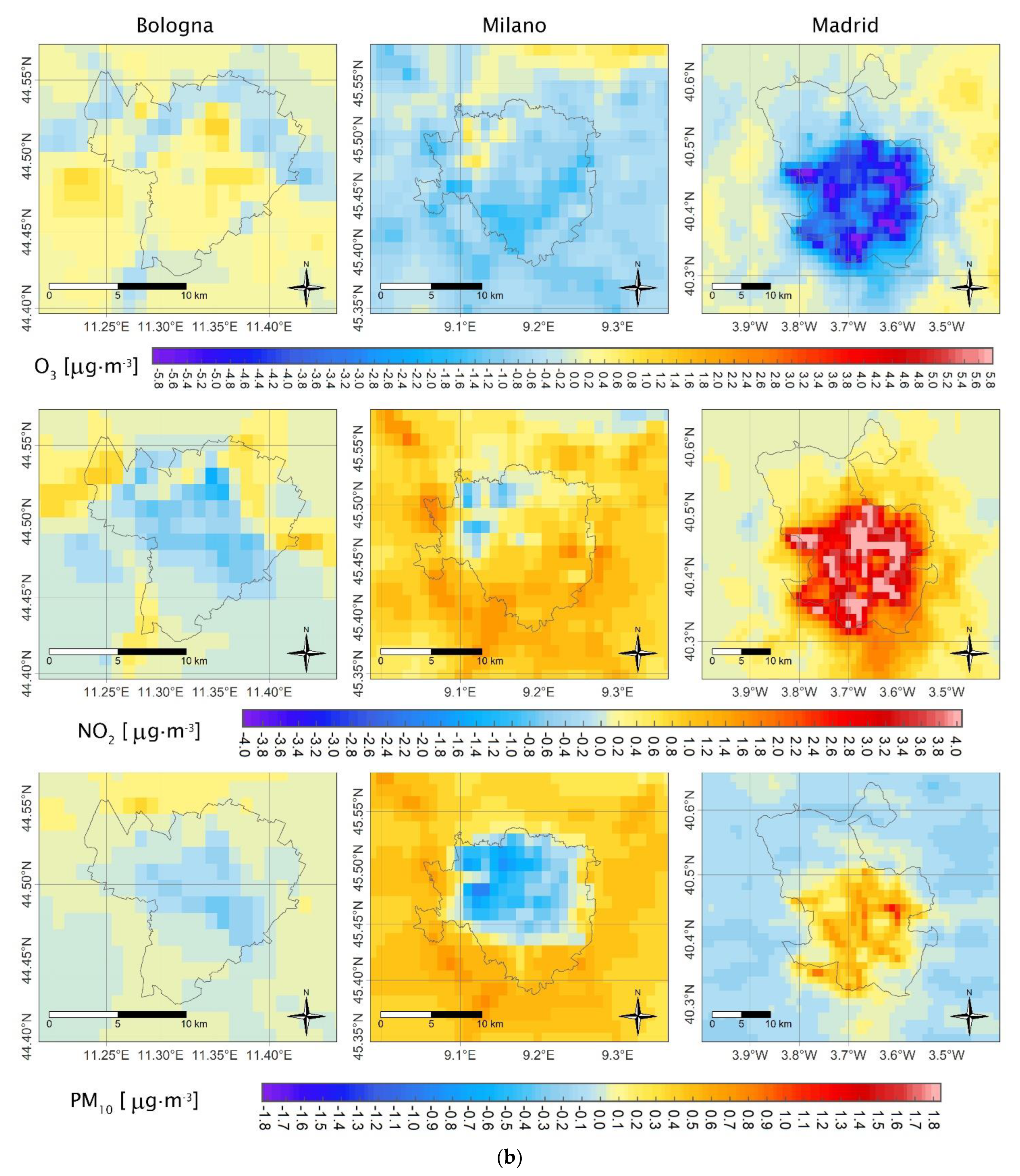
3.2. Spatial and Temporal Variability of Air Concentrations and Depositions

Figure 2a,b and Figure 3a,b show the differences between VEG and NOVEG simulations as a monthly average for air concentrations and as cumulated dry depositions, respectively. Thus, for the three pollutants investigated, the amount of pollutants removed by vegetation through the dry deposition process is directly comparable with estimates made with other simplified approaches (e.g., based on the potential absorption of each tree as an ITree model—https://www.itreetools.org/tools/i-tree-eco, accessed on 11 June 2023). Figure 2 and Figure 3 use reverse colour scales: blue to red for concentrations’ differences and red to blue for depositions’ differences. Therefore, the decrease in air concentration and the increase of dry deposition caused by vegetation is shown in blue tones (beneficial effects), and the opposite behaviour is shown using colours from yellow to red.

3.2.1. Ozone (O3)

The spatial distributions of O3 concentrations’ differences (Figure 2a,b, upper panels) reveal that the urban vegetation effects on ozone are always beneficial in Madrid; the ozone concentrations are lower for VEG than for NOVEG simulation, with the higher decrease of ozone concentrations taking place in July. In Milan, they are beneficial only in July but to a much lower extent than in Madrid and not over the whole city, while there is a slight increase of ozone concentrations (up to 0.7 mg/m3 Table 2a) in January. In Bologna, the vegetation decreases the ozone concentrations only in some grid cells, mainly located in the north of the city, in July. The ozone behaviour in Bologna is comparable to Milan in January.
The formation of ozone in the atmosphere is strongly influenced by temperature and isoprene emissions [46]. Generally, the ozone concentrations increase with the increase of temperature as it enhances the chemical kinetic rates and modifies the mechanism pathways involved in O3 formation. In the absence of the isoprene emissions’ changes, the simultaneous decrease of ozone concentrations (Figure 2a,b) and temperature (Figures 3 and 4 in D’Isidoro and Mircea et al., 2023 [11]) induced by vegetation as observed in Madrid and during summer in Milan could be expected. On the other hand, the presence of isoprene emissions in the cities may contribute to further ozone formation counteracting, thus the decrease induced by temperature. Therefore, the observed features of ozone concentrations variability in the three cities cannot be simply explained by the decrease in temperature (Figures 3 and 4 in D’Isidoro and Mircea et al., 2023 [11]) and/or by the increase in isoprene emissions (Figure 1a,b) caused by vegetation. For example, in Madrid, the highest values of ozone concentrations’ difference are not co-located in correspondence to the highest temperature differences or the highest isoprene emissions in any season.
The slight increase in ozone concentrations observed in Bologna and Milan (Figure 2a) during January may be partly explained by the persistent stagnant atmospheric conditions that usually characterise Po Valley [47] and favour the accumulation of pollutants and formation of secondary compounds such as ozone. The significant decrease in wind speed (Figures 3 and 4 in D’Isidoro and Mircea et al., 2023 [11]) due to the presence of vegetation promotes more ozone formation since the precursors are horizontally more stationary and the convection is absent. Additionally, the decrease of NO2 concentrations due to vegetation (Figure 1a) slows down the NO titration of ozone favouring the increase of O3 concentrations. Titration change seems dominant in areas where a large variation of NO2 concentration is observed. This is particularly evident in Madrid [18].
In addition to the factors discussed above, the impact of vegetation on ozone concentrations estimated here is controlled by the chemical reactions included in SAPRC99 (FARM) and CB6 (CMAQ) gas-phase mechanisms and by the chemical cocktail of anthropogenic emissions. The role of the latter can be seen in Figure S2a,b (upper panels) for all three cities: the ozone concentrations are lower in the urban areas and, particularly during summer, in correspondence of the highways, large streets with heavy traffic, etc., due to NO2 titration. Recently, new evidence proved that isoprene may also play an important role in urban areas. Zhang et al. (2021) [48] showed that removing the isoprene in a suburban area causes a decrease in ozone concentrations by slowing down reactions that involve the hydroperoxy radical (HO2), organic peroxy radical (RO2), and nitrogen oxide (NO). These radicals are also included in the two gas-phase mechanisms used here; therefore, a similar behaviour may be expected and will be investigated in detail in further studies.
The dry deposition of ozone (Figure 3a,b) interplays with all the above factors in controlling the air concentration. Therefore, an increase in dry depositions’ differences does not necessarily correspond to a decrease in air concentrations’ differences, as can be seen for January in Bologna and Milan, Figure 3a vs. Figure 2a.
The dependence of dry deposition processes on concentration itself, meteorological conditions, and land use/surface characteristics is not linear; therefore, their changes may increase or decrease the deposition resulting in positive or negative values for the differences between the two simulations. The negative values of dry deposition differences observed in the cities’ areas are caused by higher pollutant concentrations in NOVEG simulations and/or meteorological conditions more favourable for deposition; it does not mean that vegetation ceased its removal action in that grid cell.
According to Figure 3a,b, during January, in Madrid vegetation is more efficient in removing ozone than in Milan and Bologna, while the opposite behaviour is observed for July. This may be due to the presence of vegetation that remains active in winter, such as evergreen trees in Madrid (Figure S1b).
In all three urban areas, the highest monthly average vegetation contribution to O3 concentrations happens in July and ranges from −1.36 to 1.45 mg/m3 in Bologna, from −2.45 to 2.67 mg/m3 in Milan, and from −7.40 to 0.11 mg/m3 in Madrid (Table 2a). These values are more than an order of magnitude lower than the contribution of vegetation calculated on an hourly basis that may vary from −55.13 to 84.25 mg/m3 in Bologna, −61.58 to 55.26 mg/m3 in Milan, and −97.92 to 70.74 mg/m3 Madrid. The alternation of negative (beneficial effects for human health) and positive (adverse effects for human health) hourly concentrations’ differences result in lower daily, monthly, and yearly averages hiding the potential contribution of vegetation on O3 concentrations affecting human health.
Independently of averaging time, Table 2a and Figure 2a,b and Figure 3a,b show that vegetation contribution to ozone in urban areas varies significantly from one grid cell to another. The comparison of O3 concentrations and depositions’ differences (upper panels in Figure 2a,b and Figure 3a,b) with the spatial distribution of vegetation fraction and urban classes (Figure 2 in D’Isidoro and Mircea et al., 2023 [11]) shows little or no correspondence between the highest negative values of O3 concentrations’ differences and/or highest positive O3 depositions’ differences in correspondence of grid cells with the highest fraction of vegetation cover for all three cities. This behaviour confirms the non-local impact of the vegetation-induced changes on atmospheric circulation and related ozone formation processes, having a time scale of the order of hours.
As Table 2a shows for concentrations and Table 3a shows for depositions, three statistical indicators (minimum, maximum, and mean) are estimated for all grid cells within the administrative boundaries of the cities considering the monthly and yearly sums. By looking at maximum deposition on a monthly basis, it can be observed that the effect of vegetation on deposition is much higher in Bologna and Milan than in Madrid during July, and the opposite is true during January. In July, the maximum vegetation removal effect on ozone in Italian cities was five times higher than in Madrid in some cells (524.27 and 561.35 kg/m2 with respect to 112.03 kg/m2). On a yearly basis, the difference in vegetation effects between the cities decreases by a factor of two.
Comparing the mean and maximum amount of ozone removed by vegetation (VEG-NOVEG) with those removed by all surfaces (VEG), total dry deposition (Table 3a), it can be observed that the maximum effect of vegetation removal is comparable with the minimum of total dry deposition. Additionally, the ozone removed by vegetation (max VEG-NOVEG) with respect to total ozone removed (max VEG) varies from 17% to 40%, with the lowest values in January in Bologna and the highest in July in Milan.

3.2.2. Nitrogen Dioxide (NO2)

Figure 2a,b (middle panels) show the spatial distributions of NO2 concentrations’ differences attributable to urban vegetation. As expected from the formulation of gas-phase chemical mechanisms, their patterns are complementary to those of O3 concentrations’ differences (Figure 2a,b upper panels); positive O3 values correspond to negative NO2 values and vice versa. In Madrid, the presence of vegetation leads to an increase of NO2 concentrations over most of the urban area, more extended and intense during July, in some grid cells for more than 4 mg/m3 (maximum value 7.17 mg/m3 Table 2b). In Bologna and Milan, the NO2 concentrations exhibit also decreases over a more extended area in Bologna than in Milan in winter. This feature is maintained during summer in Bologna, while in Milan, NO2 shows increasing values over a large part of the municipality. It is worth noticing that the sign of concentration changes and the spatial distribution of values is quite coherent for NO2 and PM10 in all cities during winter when BVOC emissions are reduced to very low values, chemistry has a minor impact, and concentrations are high. This general coherence is lost during summer, with differences in the studied cities. Similar patterns are maintained in the central part of Madrid, while a change of sign can be observed in the peripheral areas; Milan shows a reduction of PM10 and an increase of NO2 over a large part of the city (Figure 2b,c). This behaviour suggests a prevailing impact of the combination of an increase in deposition and decrease of wind speed caused by vegetation during winter, with a similar impact on NO2 and primary PM, while the complex combination of the atmospheric circulation change, deposition, and atmospheric chemistry causes different results in the different cities. The higher effect of vegetation on NO2 concentrations in Madrid with respect to Bologna and Milan can be due to the fact that the highest NO2 concentrations (VEG) are mainly in the city area, as shown in Figure S2a,b. On the other hand, especially during January, Bologna and Milan show high NO2 concentrations (VEG) over the whole domain, not only over the city area, thus limiting the removal power of urban vegetation. As for ozone, the sign and pattern of these differences show no similarity with the spatial distribution of vegetation fraction or/and urban classes (Figure 2 in D’Isidoro and Mircea et al., 2023 [11]). While Figure S2a,b clearly shows high NO2 concentrations in correspondence with traffic emissions in all three cities (VEG simulations), no such pattern is evident in the monthly averaged differences VEG-NOVEG (Figure 2a,b middle panels). However, on a daily basis, for a summer day (13 July) in the middle of a period of high-pressure conditions, Mircea et al. (2022) [49] showed that the differences in O3 and NO2 concentrations and depositions due to vegetation are higher along A1 and A14 highways (NW-SE and south directions) than in other areas of Bologna. This is clear evidence of high vegetation impact in areas with high concentrations. On a monthly basis, this relationship “disappears” since the concentrations vary not only due to traffic emissions, the major source on a sunny stable day, but also due to transport and dispersion, formation, and destruction process, etc., from other emission sources, including vegetation, and processes controlled by meteorological changes. In the case of the other two cities, the NO2 differences in concentration do not show a relationship with traffic emissions, probably due to the cities’ morphology.
During July, Table 2b shows that the beneficial vegetation effect (VEG-NOVEG) on NO2 concentrations is significant on an hourly basis being, in most cases, comparable with maximum NO2 concentrations given by VEG simulation. As for O3, the differences in NO2 concentrations are highest on an hourly basis (tens of mg/m3 with maximum reduction in July in the Bologna area: −87.34 mg/m3). It is interesting to note that during July, when the vegetation is most active, due to the decrease in wind speed [11] and PBL (Figure S3), vegetation also leads to an increase in concentrations, with the maximum increase observed in Madrid, 126.98 mg/m3 on an hourly basis. On a monthly basis, it is important to note the non-homogeneous effect of vegetation on NO2 concentrations spanning several mg/m3, even in adjacent grid cells, sometimes alternating positive and negative effects (Figure 2a,b middle panels). The overall monthly mean impact remains beneficial in Bologna, while a prevailing increase of concentrations is obtained for Milan and Madrid (Figure 2b and Table 2b).
The differences in the dry deposition of NO2 (Figure 3a,b, middle panel) are comparable to those observed for ozone (upper panel) in January but lower in July. In Bologna and Milan, the maximum amount of NO2 removed represents ca. 25 and 14 %, respectively, of the maximum amount of O3 removed (Table 3a,b). This is partly explained by the pollutant availability in the air: the concentrations of O3 are much higher than the concentrations of NO2 (Figure S2a,b). The NO2 is emitted by anthropogenic sources, mainly by traffic; therefore, the amount released in the atmosphere is almost the same, independent of season, leading to similar concentrations, while O3 is formed in the atmosphere on sunny hot days, increasing substantially during summer. Additionally, the surface resistances of O3 are computed in a different way from NO2 by AMS-MINNI, considering the effect of dew and rain on leaves as suggested by [38]. For each city, for a given month, the patterns of differences in NO2 and O3 are alike but not clearly attributable to the presence of vegetation. Only in Madrid is it easy to note an area with high deposition in the southeast of the city in correspondence of HR urban class (Figure 2 in D’Isidoro and Mircea et al., 2023 [11]) in all seasons (Figure 3a,b, upper and middle panels).
As for O3, it can be noticed for all three cities that the vegetation effects on NO2 depositions are higher in summer than winter (Table 3a), the highest variability within the city’s area being observed in Bologna: from −3.21 to 132.63 kg/km2 (VEG-NOVEG). Among the three cities investigated, the NO2 removed by vegetation (max VEG-NOVEG) with respect to total NO2 removed (max VEG) has the highest value in Madrid, ca. 77% in July, followed by Milan, ca. 53%, and Bologna, 38%. Despite this high removal vegetation efficiency in Madrid, Figure 2 and Table 2 show an increase in NO2 concentrations in both months. This may be explained by the observed decrease of O3 concentrations (Figure 2) because of isoprene emissions’ increase in VEG simulation and even by the decrease of wind speed reducing dispersion of local emissions [11]. The negative sensitivity of O3 to isoprene emissions when using the CB6 gas mechanism in CMAQ was shown in [50].

3.2.3. Particulate Matter (PM10)

Over extended areas, the differences in PM10 concentrations due to vegetation (Figure 2a,b, lower panels) have negative values in Bologna and Milan and positive values in Madrid during both winter and summer. In the Italian cities, the reduction of the concentrations expressed as monthly mean (Table 2c) is up to −3.14 mg/m3 in Milan, while in Madrid, an increase up to 1.32 mg/m3 is observed. In Bologna and Madrid, almost everywhere, for both months, it is interesting to note the similarity of vegetation effects on PM10 and NO2 concentrations: they simultaneously decrease in Bologna and increase in Madrid. This may be since part of PM10 is directly emitted into the atmosphere as primary particles by the same sources as NO2, traffic, and domestic heating, while another part, such as ammonium nitrate (NH4NO3), is formed in the atmosphere through reactions involving NO2 availability. In Madrid, in January, we also observed a decrease in concentrations (negative values) for both pollutants in the southeast area of the city in correspondence with high residential (HR) urban classes (Figure 2 in [11]). In this area, we observed an increase of planetary boundary layer (PBL) height in VEG simulation (positive values in Figure S3, upper panel, left map) that may lead locally to a decrease of concentration through dilution. The relationship between PBL height-concentration is not always dominant. For the same decrease of PBL height, in Milan, in July, the vegetation has opposite effects on the two pollutants, causing an increase of NO2, as expected, but a decrease of PM10 concentrations. This may be explained by a more efficient PM10 removal, more effective dispersion/transport outside the city area, and/or less efficient formation of secondary aerosol particles. Otherwise, the PM10 concentration should increase at least for the two following reasons: (i) the concentrations of PM10, in particular, the primary part of PM10 mainly released by traffic, should increase when PBL height decreases, similarly with NO2, and (ii) the concentration of secondary organic aerosol comprised in PM10 should increase due to the increase of its precursors BVOC emissions (Figure 1a,b).
The variability of vegetation effects on PM10 concentrations from one grid cell to another within the city area is significant, as shown in Figure 2a,b for all three cities, and it is much higher on an hourly basis: in Milan, it leads to a decrease up to −95.79 μg/m3 and to an increase up to 112.45 mg/m3, in January.
As for O3 and NO2, the monthly sum of differences (VEG-NOVEG) of PM10 dry depositions (Figure 3a,b, bottom panel) due to vegetation are higher in July than in January, and the highest values are observed in Milan, up to a maximum of 256.62 kg/km2 on a monthly basis representing ca. 29% of maximum deposition 889.16 kg/km2 (Table 3c). For the same month, July, in Bologna and Madrid, the statistics relative to the effects of vegetation on PM10 deposition are more similar, the maximum depositions’ differences being 88.48 and 87.05 kg/km2, respectively, and representing ca. 37% and 45%, respectively, of maximum depositions of 239.96 kg/km2 and 192.66 kg/km2 (Table 3c).

3.3. Pollutants’ Concentrations and Depositions in Relation to Land-Use Classes and Vegetation Fraction

Figure 4 shows some statistics of the hourly variation of concentrations (rows 1, 3, and 5) and depositions’ (rows 2, 4, and 6) differences due to vegetation for urban (HR, HL, and CI) and vegetation classes in Bologna (columns 1–2), Milan (columns 3–4), and Madrid (columns 5–6), respectively.
Overall, several common features are observed in the hourly variations of vegetation effects: (i) for all three pollutants investigated and for all three cities, the shaded area covering the interval 10th to 90th percentiles is much larger during July than during January, despite pollutants concentrations being significatively higher during winter, confirming the important role of vegetation on atmosphere during the warm season (red areas with respect to the blue ones), except PM10 concentrations differences in Bologna and Milan where the opposite is true (column 5, rows 1–2) and where winter concentration of PM10 is much higher than in Madrid (Figure S2a); (ii) the differences have higher values in urban cells than in vegetation cells in all graphs, for all pollutants in all three cities (this may be partly due to the way the numerical experiment was designed, in particular the meteorological simulation that did not consider the vegetation only in urbanised cells in NOVEG simulation); (iii) the depositions are higher during the day (6–21 h) for all pollutants in all three cities, with two peaks for NO2 in all three cities and for PM10 in Madrid. The absence of the two peaks for PM10 in Bologna and Milan indicates a lower relative weight of traffic emissions for this pollutant.
It should also be noted that the magnitude of the daily cycles of 10th and 90th percentiles differences vary with pollutants (O3, NO2, and PM10) and cities both for concentrations and depositions. For O3 hourly concentrations’ differences, Madrid exhibits the highest variability (Table 2a), followed by Milan and Bologna, which are comparable and similar in shape. However, their shapes and magnitude show no resemblance with the bell shapes aspect of isoprene and BVOC emissions (Figure S5). In the case of deposition, Madrid shows lower variability than the other two cities: 0.3 and 0.9 kg/km2, respectively. In Madrid, it is also interesting to note a fast and well-defined decline of O3 concentrations around 18:00 hrs (up to −40 mg/m3), probably due to NO titration in correspondence with NO2 concentration increase (up to 40 mg/m3). This suggests that the O3 decrease is mainly driven by gas chemical reactions, also because the removal due to vegetation is less efficient than in the other two cities where such a substantial decrease is not observed.
In July, in particular, in both Italian and Spanish cities, a similar shape for the daily cycle of deposition differences is observed for NO2, with two maxima in the morning and afternoon in correspondence with the maximum of traffic emissions, respectively. There is no such evident behaviour in the daily cycles of concentrations’ differences for this pollutant.
However, it can be noted that Bologna and Milan have similar daily variations (shaded areas) in shape but are different from Madrid for all pollutants. The first reason for that could be the use of different photochemistry (SAPRC99 vs. CB6), followed by the different chemical regimes due to emissions and by the peculiarities in cities’ morphology. These may also explain the differences observed between PM10 daily cycles of concentration in Madrid vs. Italian cities: only the former has well-defined peaks in correspondence with the morning and afternoon maximum traffic emissions in both months. However, despite all the differences between the applications of the two AMS, it is interesting to note a decrease of PM10 between 9 and 12 h in urban cells in all three cities.
For all land use classes, for Bologna, the daily cycles of concentrations and depositions’ differences are shown in Figure S4ac1 for O3, S4ac2 for NO2, S4ac3 for PM10, and Figure S4ad1 for O3, S4ad2 for NO2, S4ad3 for PM10, respectively. Similarly, for Milan in Figure S4bc1, bc2, bc3 and Figure S4bd1, bd2, bd3, and for Madrid in Figure S4cc1, cc2, cc3 and Figure S4cd1, cd2, cd3. As for the urban classes, the shapes of the daily cycles of differences induced by vegetation do not show a striking dependence on land use classes, but there are some differences in the magnitude. It is interesting to note that the highest effects of vegetation on both concentrations and depositions’ differences in daily cycles exist in urban classes in all three cities for all three pollutants. Those corresponding to other land use classes are lower or similar but not higher.
For each urban class, the hourly variability of concentrations and depositions’ differences of the three pollutants investigated in relation to vegetation fraction is shown in Figure S6 respectively. At a glance view of Figure S6, it can be noticed that no relationships exist between the concentrations’ differences and vegetation fraction: the boxplots have similar sizes for a given pollutant in a given city. The dependence on the urban class is also inexistent. Again, for O3 and NO2 in all three cities, we confirmed the higher variability in July than in January (cyan boxes higher than the red ones). For PM10, Madrid shows comparable variability of concentrations’ differences for both months, while Bologna and Milan have higher variability in January than in July (opposite behaviour with respect to O3 and NO2).
The depositions’ differences of the three pollutants investigated in relation to vegetation fraction (Figure S6) show for all urban classes and for all three cities higher variability in July than in January. In some cases, they also show an increase of depositions’ differences with the increase of vegetation fraction but not always. In Madrid, in particular, for all three pollutants, in most cases, the boxplots size is almost the same for all vegetation fractions. In Bologna and Milan, we often observed a decrease in boxplot size at high vegetation fractions. This is the result of removal characteristics of vegetation, of meteorological and chemical changes of atmospheric conditions due to vegetation, and dry deposition approaches used in the two AMS. It is worth recalling that the VEG and NOVEG simulations produced two independent atmospheres characterised by two different meteorological conditions and two different distributions of air concentrations and depositions due to the presence and absence of vegetation, respectively. Therefore, in a grid cell, the VEG concentration may be lower than the NOVEG concentration, and, consequently, the VEG deposition is lower than the NOVEG deposition because the dry deposition process is directly dependent on concentration. This explains the negative values of depositions’ differences. The cleaning effect of vegetation exists, but due to its proportionality to the air concentration, it does not produce a higher deposition in the VEG simulation than in the NOVEG simulation.
For all cities and pollutants, we observed a large variability of the whiskers spanning the interval 10th to 90th percentile of depositions’ differences, evidencing that vegetation effects are highly variable in time and space in agreement with the high spatial variability shown in Figure 3a,b. The same observation is valid for Figure 2a,b and Figure S6a showing concentrations’ differences.

3.4. Overall Discussion of Results

The comparison of the spatial distribution of air concentrations differences in the three cities (Figure 2a,b) shows that the averaged vegetation effects are highly variable from one grid cell to another in the city area, with positive and negative effects or high/low effects in adjacent cells being observed for all three polluted investigated. The vegetation effects’ patterns and their magnitude vary from city to city for all pollutants investigated. According to pollutants, on a monthly basis, extreme differences exist in July for O3 (−7.40 mg/m3 in Madrid and +2.67 mg/m3 in Milan) and NO2 (−3.01 mg/m3 in Milan and +7.17 mg/m3 in Madrid) and in January for PM10 (−3.14 mg/m3 in Milan and +2.01 mg/m3 in Madrid) (monthly minimum and maximum in Table 2a–c). These values and the graphs clearly visualize the opposite behaviour of vegetation effects on O3 and NO2 as expected from the formulation of photochemical gas-phase mechanisms: an increase of O3 corresponds to a decrease of NO2 and vice versa. The magnitude of the concentrations’ differences is partly due to the photochemical mechanism of each CTM of AMS (higher values in Madrid with respect to Italian cities for O3Figure 2a,b) and partly due to specific meteorological and chemical conditions of the city (different O3 values in Milan vs. Bologna in July—Figure 2b). PM10 concentrations’ differences in January seem relatively similar to NO2 patterns, even if they include the effects of different formulations of aerosol dynamics and chemistry in the two CTMs of AMS, in addition to different gas-phase mechanisms. This suggests a small impact of BVOC precursors emissions on the PM10 through SOA formation.
However, the magnitude of the concentrations’ differences is primarily dependent on averaging periods, and longer periods produce lower values, as shown in Table 2, since positive and negative values are summed. Thus, the highest effect of vegetation on concentrations is obtained on an hourly basis and amounts to tens of mg/m3 for all three pollutants in both months, being higher during July than January, as expected due to intense vegetation activity.
The pattern of depositions’ differences (Figure 3a,b) shows almost everywhere and is always an important removal effect of vegetation (positive values). The existence of negative values was explained in Section 3.3. For a given city and a given month, the vegetation effect on depositions of O3 and NO2 is similar as a pattern but not as a magnitude and is different from those of PM10. These differences may be due to different parametrizations of dry deposition of gases and aerosols in the two CTMs of AMS. According to pollutants, on a monthly basis, the highest depositions’ differences exist in July for O3 and PM10, being 561.35 kg/km2 and 256.62 kg/km2 in Milan, and for NO2, 132.63 kg/km2 in Bologna (Table 3a–c).
Overall, for both months, the vegetation effects on concentrations of these three interdependent pollutants can be summarized as being mostly beneficial for O3 in Madrid and for PM10 in Bologna and Milan (negative values in Figure 2a,b).
The increase of planetary boundary layer (PBL) height in VEG simulation (positive values in Figure S3, upper panel, left map) may lead locally to a decrease of concentration through dilution. The growth of PBL is due to increased mechanical or thermodynamic turbulence: turbulence improves the efficiency of dry deposition removal but also increases dilution. The differences in concentrations depend mostly on the relative strength of the two effects. However, this relation between the effect of vegetation on PBL height and pollutant concentrations is not verified in the case of ozone in Madrid, where the ozone concentrations decrease even when the PBL height decreases both in January and July. Additionally, in Bologna and Milan, PBL heights always undergo substantial decreases, but those correspond to both decreases and increases in pollutants’ concentrations. The interplay between meteorological and chemical conditions changes to transport, formation and destruction, and removal processes. Therefore, there is no simple way to relate the vegetation impact of meteorological parameters (also those shown in Figures 3 and 4 of D’Isidoro and Mircea, 2023, [11]) on concentrations or on depositions.

4. Conclusions

This study shows that the vegetation impact on air concentrations of O3, NO2, and PM10 is highly variable within the city’s area and is not always beneficial, leading to an increase in concentrations (noteworthy is the increase of NO2 and PM10 in Madrid). The comparison between the spatial distribution of concentrations and dry depositions does not show a decrease of concentrations in correspondence with a large amount of pollutant deposited. As for the differences in concentrations, the differences in dry depositions show large variability across the city’s area but without a clear dependence on vegetation fraction. As expected, the magnitude of vegetation effects on both concentrations and depositions depends on the season being higher during July when vegetation is more active than in January.
The intercomparison of differences in air concentrations and deposition in the three cities (Bologna, Milan, and Madrid) shows in an unequivocal way that the response of air quality parameters to the presence of vegetation is city-dependent and cannot be predicted without AMS simulations. While the impact of vegetation on temperature is almost always the same, a cooling effect on air quality is more complex since, in addition to meteorology, it is strongly dependent on the anthropogenic emissions cocktail. Thus, the impact of BVOC emission, in particular of isoprene on ozone concentrations, depends on the anthropogenic VOC/NOx ratio. Moreover, the decrease in temperature and the increase in isoprene are two counteracting factors in O3 formation that explain the positive and negative sensitivity of O3 with BVOC emissions. The daily cycles of the differences in air concentrations and deposition in the three cities vary with pollutants (O3, NO2, and PM10) and city and have higher values in the cells dominated by urban fraction than those dominated by vegetation. Another common feature of the three cities is that the depositions are higher during daytime (6–21 h) for all pollutants.
Due to the alternate positive and negative values for differences in air concentrations of pollutants, the magnitude of vegetation impact evaluated as the average of concentrations’ differences is diminished when considering longer periods and months, as shown here. Thus, the effect of vegetation on concentrations varies from decimals to tens of mg/m3 when evaluated on a monthly and hourly basis, respectively, for all three pollutants, being higher during July than January, as expected due to intense vegetation activity.
Ongoing work is in progress to separately quantify the impact of meteorology and BVOC emissions on air quality in Bologna and Milan cities.
The present methodological approach focuses only on the effect of urban vegetation assessed in the most realistic possible way as a base for further experimental and theoretical investigations by the atmospheric scientific community. It also provides more detailed and reliable information to assess the human health impacts of vegetation on the urban population.
The vegetation impact on air quality in the urban atmosphere is highly variable in time and space and reflects the combined effect of the vegetation itself, urban morphology, and meteorology in addition to anthropogenic emissions. Future applications of the VEG-GAP approach in other cities will allow us to better understand how combined urban vegetation morphology affects the atmosphere. This is important since they are key elements of architectural projects and act together as an atmospheric forcer. Therefore, urban planning and air quality plans may use this approach for designing no-regret strategies for the further development of cities.

Supplementary Materials

The following supporting information can be downloaded at: https://www.mdpi.com/article/10.3390/f14061255/s1, Table S1: FARM and CMAQ CTMs domains used for simulations from continental to urban scale; Table S2: FARM and CMAQ validation of VEG simulations from continental to urban scale; Table S3: Ranking of the 20 most relevant species in terms of percent of the total area covered by trees. Colours identify the same species in different cities; Figure S1. Fractional land cover maps of deciduous broadleaf species (left), evergreen needleleaf evergreen species (centre) and grass (right panel) over Bologna urban area (black contour). Maps are obtained as difference of vegetation cover characterising VEG and NOVEG scenarios. Pixel dimension is 1 km2. Colour scales are different to make the maps of different vegetation classes. visible.(a) Bologna, (b) Milano, (c) Madrid; Figure S2. Monthly averages of air concentrations (g/m3) (VEG) for O3 (upper panel), NO2 (middle panel) and PM10 (bottom panel) in Bologna (left column), Milan (central column) and Madrid (right column) (a) January 2015, (b) July; Figure S3: Monthly averages of differences (VEG-NOVEG) of planetary boundary layer (PBL) height (m) for January (upper panel) and July (bottom panel) in Bologna (left column), Milan (central column), and Madrid (right column); Figure S4: Description of multiple graphs with the daily cycle of O3, NO2, and PM10 concentration differences (VEG-NOVEG) (μg/m3) and deposition differences (VEG-NOVEG) (kg/km2) as a function of land use, considering only grid points inside the municipalities; Figure S5: Daily cycle of BVOC emissions differences (VEG-NOVEG) (kg/km2) as a function of land-use, considering only grid points inside the municipality for Bologna, Milan and Madrid from left to right. Medians are shown as lines and shaded area covers the interval 10th to 90th percentiles. Cyan and red colours refer to July and January, respectively; Figure S6: Boxplots of concentration (g/m3) and deposition (kg/km2) differences (VEG-NOVEG) for O3 (upper panels), NO2 (middle panel) and PM10 (bottom panels) as a function of vegetation fraction for different land-use classes, considering only grid points inside the Bologna (left column), Milan (middle column) and Madrid (left column) municipalities. Whiskers span the interval 10th to 90th percentile. Red (blue) colour refers to July (January).

Author Contributions

Conceptualization: M.M.; methodology: M.M., S.F. and R.B.; software: M.M., M.D., C.S., G.B., F.R., D.d.l.P., M.G.V., A.C., M.A., B.S., N.P., R.P. and G.C. (Giuseppe Carlino); validation: G.B., D.d.l.P., M.G.V., A.C., M.A., R.P. and G.C. (Giuseppe Carlino); formal analysis M.M.; investigation: M.M., S.F., R.P. and G.B.; resources: M.M., R.B., S.F., D.d.l.P., M.D., I.D., A.P., E.P. and R.P.; data curation: M.M., G.B., G.C. (Giuseppe Cremona), A.C., M.A., E.P., J.M.d.A., A.N., N.P. and R.P.; data acquisition: M.M., S.F., M.D., R.B., D.d.l.P. and G.C. (Giuseppe Cremona); writing—original draft preparation: M.M.; writing—review and editing: M.M., M.D., S.F., C.S., R.B., G.B., F.R., D.d.l.P., I.D., E.P., R.P. and G.C. (Giuseppe Carlino); visualization: M.M., M.D., F.R., G.B., M.G.V., M.A. and G.C (Giuseppe Carlino); supervision: M.M., R.B. and S.F.; project administration: M.M.; funding acquisition: M.M. All authors have read and agreed to the published version of the manuscript.

Funding

This study was developed under the project Life VEG-GAP (https://www.lifeveggap.eu/ Accessed 15 May 2023) and funded by the European Union Life Program in 2018, Grant Number LIFE18 PRE IT 003.

Data Availability Statement

The datasets generated during and/or analysis during the current study are not publicly available due to the high volume of data but are available from the corresponding author upon reasonable request. Data analysis products are available on the information platform: https://veggaplatform.enea.it (accessed on 15 May 2023).

Acknowledgments

We acknowledge the support of Madrid and Milan Municipalities and the Metropolitan City of Bologna in the acquisition of tree inventories in the framework of the Life VEG-GAP project (www.lifeveggap.eu, accessed on 11 June 2023). The computing resources and the related technical support used for this work have been provided by CRESCO/ENEAGRID High-Performance Computing infrastructure and its staff . CRESCO/ENEAGRID High-Performance Computing infrastructure is funded by ENEA, the Italian National Agency for New Technologies, Energy and Sustainable Economic Development, and by Italian and European research programmes; see http://www.cresco.enea.it/english (accessed on 14 May 2023) for information. We also acknowledge Madrid’s Air Quality Service for providing a meteorological dataset from the City Hall meteorological network, Regional Agency for Prevention, Environment and Energy of Emilia-Romagna, and of Lombardy for providing the anthropogenic emission inventory for Bologna and Milan, TNO (Nederlandse Organisatie voor Toegepast Natuurwetenschappelijk Onderzoek) for providing the European anthropogenic emissions CAMS-REG-AP_v2.2.1 and ECMWF (European Centre for Medium-Range Weather Forecasts) for providing European meteorological data (DSC-9674 Permission to use IFS data).

Conflicts of Interest

The authors declare no conflict of interest. The funders had no role in the design of the study; in the collection, analyses, or interpretation of data; in the writing of the manuscript; or in the decision to publish the results.

References

  1. United Nations, Department of Economic and Social Affairs, Population Division. World Urbanization Prospects: The 2018 Revision (ST/ESA/SER.A/420); United Nations: New York, NY, USA, 2019. [Google Scholar]
  2. Dudareva, N.; Negre, F.; Nagegowda, D.A.; Orlova, I. Plant Volatiles: Recent Advances and Future Perspectives. Crit. Rev. Plant Sci. 2006, 25, 417–440. [Google Scholar] [CrossRef]
  3. Bodnaruk, E.W.; Kroll, C.N.; Yang, Y.; Hirabayashi, S.; Nowak, D.J.; Endreny, T.A. Where to Plant Urban Trees? A Spatially Explicit Methodology to Explore Ecosystem Service Tradeoffs. Landsc. Urban Plan. 2017, 157, 457–467. [Google Scholar] [CrossRef] [Green Version]
  4. Oxley, T.; Dore, A.J.; ApSimon, H.; Hall, J.; Kryza, M. Modelling Future Impacts of Air Pollution Using the Multi-Scale UK Integrated Assessment Model (UKIAM). Environ. Int. 2013, 61, 17–35. [Google Scholar] [CrossRef] [PubMed] [Green Version]
  5. Manes, F.; Marando, F.; Capotorti, G.; Blasi, C.; Salvatori, E.; Fusaro, L.; Ciancarella, L.; Mircea, M.; Marchetti, M.; Chirici, G.; et al. Regulating Ecosystem Services of Forests in Ten Italian Metropolitan Cities: Air Quality Improvement by PM10 and O3 Removal. Ecol. Indic. 2016, 67, 425–440. [Google Scholar] [CrossRef]
  6. Abhijith, K.V.; Kumar, P.; Gallagher, J.; McNabola, A.; Baldauf, R.; Pilla, F.; Broderick, B.; Sabatino, S.D.; Pulvirenti, B. Air Pollution Abatement Performances of Green Infrastructure in Open Road and Built-up Street Canyon Environments—A Review. Atmos. Environ. 2017, 162, 71–86. [Google Scholar] [CrossRef]
  7. Karttunen, S.; Kurppa, M.; Auvinen, M.; Hellsten, A.; Järvi, L. Large-Eddy Simulation of the Optimal Street-Tree Layout for Pedestrian-Level Aerosol Particle Concentrations—A Case Study from a City-Boulevard. Atmos. Environ. X 2020, 6, 100073. [Google Scholar] [CrossRef]
  8. Khan, B.; Banzhaf, S.; Chan, E.C.; Forkel, R.; Kanani-Sühring, F.; Ketelsen, K.; Kurppa, M.; Maronga, B.; Mauder, M.; Raasch, S.; et al. Development of an Atmospheric Chemistry Model Coupled to the PALM Model System 6.0: Implementation and First Applications. Geosci. Model Dev. 2021, 14, 1171–1193. [Google Scholar] [CrossRef]
  9. Geletič, J.; Lehnert, M.; Resler, J.; Krč, P.; Middel, A.; Krayenhoff, E.S.; Krüger, E. High-Fidelity Simulation of the Effects of Street Trees, Green Roofs and Green Walls on the Distribution of Thermal Exposure in Prague-Dejvice. Build. Environ. 2022, 223, 109484. [Google Scholar] [CrossRef]
  10. San Jose, R.; Perez-Camanyo, J.L. High-Resolution Impacts of Green Areas on Air Quality in Madrid. Air Qual. Atmos. Health 2023, 16, 37–48. [Google Scholar] [CrossRef]
  11. D’Isidoro, M.; Mircea, M.; Borge, R.; Finardi, S.; de la Paz, D.; Briganti, G.; Russo, F.; Cremona, G.; Villani, M.G.; Adani, M.; et al. The Role of Vegetation on Urban Atmosphere of Three European Cities. Part 1: Evaluation of Vegetation Impact on Meteorological Conditions. Forests 2023, 14, 1235. [Google Scholar] [CrossRef]
  12. Mircea, M.; Ciancarella, L.; Briganti, G.; Calori, G.; Cappelletti, A.; Cionni, I.; Costa, M.; Cremona, G.; D’Isidoro, M.; Finardi, S.; et al. Assessment of the AMS-MINNI System Capabilities to Simulate Air Quality over Italy for the Calendar Year 2005. Atmos. Environ. 2014, 84, 178–188. [Google Scholar] [CrossRef]
  13. Mircea, M.; Grigoras, G.; D’Isidoro, M.; Righini, G.; Adani, M.; Briganti, G.; Ciancarella, L.; Cappelletti, A.; Calori, G.; Cionni, I.; et al. Impact of Grid Resolution on Aerosol Predictions: A Case Study over Italy. Aerosol Air Qual. Res. 2016, 16, 1253–1267. [Google Scholar] [CrossRef] [Green Version]
  14. Adani, M.; Piersanti, A.; Ciancarella, L.; D’Isidoro, M.; Villani, M.G.; Vitali, L. Preliminary Tests on the Sensitivity of the FORAIR_IT Air Quality Forecasting System to Different Meteorological Drivers. Atmosphere 2020, 11, 574. [Google Scholar] [CrossRef]
  15. D’Elia, I.; Briganti, G.; Vitali, L.; Piersanti, A.; Righini, G.; D’Isidoro, M.; Cappelletti, A.; Mircea, M.; Adani, M.; Zanini, G.; et al. Measured and Modelled Air Quality Trends in Italy over the Period 2003–2010. Atmos. Chem. Phys. 2021, 21, 10825–10849. [Google Scholar] [CrossRef]
  16. Saiz-Lopez, A.; Borge, R.; Notario, A.; Adame, J.A.; de la Paz, D.; Querol, X.; Artíñano, B.; Gómez-Moreno, F.J.; Cuevas, C.A. Unexpected Increase in the Oxidation Capacity of the Urban Atmosphere of Madrid, Spain. Sci. Rep. 2017, 7, 45956. [Google Scholar] [CrossRef] [Green Version]
  17. Borge, R.; Santiago, J.L.; de la Paz, D.; Martín, F.; Domingo, J.; Valdés, C.; Sánchez, B.; Rivas, E.; Rozas, M.T.; Lázaro, S.; et al. Application of a Short Term Air Quality Action Plan in Madrid (Spain) under a High-Pollution Episode—Part II: Assessment from Multi-Scale Modelling. Sci. Total Environ. 2018, 635, 1574–1584. [Google Scholar] [CrossRef]
  18. de la Paz, D.; de Andrés, J.M.; Narros, A.; Silibello, C.; Finardi, S.; Fares, S.; Tejero, L.; Borge, R.; Mircea, M. Assessment of Air Quality and Meteorological Changes Induced by Future Vegetation in Madrid. Forests 2022, 13, 690. [Google Scholar] [CrossRef]
  19. Ciccioli, P.; Silibello, C.; Finardi, S.; Pepe, N.; Ciccioli, P.; Rapparini, F.; Neri, L.; Fares, S.; Brilli, F.; Mircea, M.; et al. The Potential Impact of Biogenic Volatile Organic Compounds (BVOCs) from Terrestrial Vegetation on a Mediterranean Area Using Two Different Emission Models. Agric. For. Meteorol. 2023, 328, 109255. [Google Scholar] [CrossRef]
  20. Skamarock, W.C.; Klemp, J.B.; Dudhia, J.; Gill, D.O.; Barker, D.; Duda, M.G.; Huang, X.-Y.; Wang, W.; Powers, J.J. A Description of the Advanced Research Wrf Version 3; UCAR: Boulder, CO, USA, 2008. [Google Scholar]
  21. Skamarock, W.C.; Klemp, J.B.; Dudhia, J.; Gill, D.O.; Liu, Z.; Berner, J.; Wang, W.; Powers, J.J.; Duda, M.G.; Barker, D.; et al. A Description of the Advanced Research Wrf Model Version 4.1; UCAR: Boulder, CO, USA, 2019. [Google Scholar]
  22. ARIA/ARIANET. Emission Manager-Processing System for Model-Ready Emission Input-User’s Guide. R2013.19; ARIA/ARIANET: Milan, Italy, 2013; Available online: https://www.afs.enea.it/forecast/R2013.19-EmissionManager_manual.eng.pdf (accessed on 15 May 2023).
  23. Baek, B.H.; Seppanen, C. Sparse Matrix Operator Kernel Emissions (SMOKE) Modeling System (Version SMOKE User’s Documentation); 2018. Available online: https://www.cmascenter.org/smoke/ (accessed on 15 May 2023).
  24. Silibello, C.; Calori, G.; Brusasca, G.; Giudici, A.; Angelino, E.; Fossati, G.; Peroni, E.; Buganza, E. Modelling of PM10 Concentrations over Milano Urban Area Using Two Aerosol Modules. Environ. Model. Softw. 2008, 23, 333–343. [Google Scholar] [CrossRef]
  25. Byun, D.; Schere, K.L. Review of the Governing Equations, Computational Algorithms, and Other Components of the Models-3 Community Multiscale Air Quality (CMAQ) Modeling System. Appl. Mech. Rev. 2006, 59, 51–77. [Google Scholar] [CrossRef]
  26. Carter, W.P.L. Documentation of the SAPRC-99 Chemical Mechanism for VOC Reactivity Assessment. Final Report to California Air Resources Board. In Final Report to California Air Resources Board. 2000. Available online: https://intra.engr.ucr.edu/~carter/pubs/s99doc.pdf (accessed on 15 May 2023).
  27. Emery, C.; Jung, J.; Koo, B.; Yarwood, G. Improvements to CAMx Snow Cover Treatments and Carbon Bond Chemical Mechanism for Winter Ozone; 2015. Available online: https://www.camx.com/files/udaq_snowchem_final_6aug15.pdf (accessed on 15 May 2023).
  28. Binkowski, F.S.; Roselle, S.J. Models-3 Community Multiscale Air Quality (CMAQ) Model Aerosol Component 1. Model Description. J. Geophys. Res. 2003, 108, 2001JD001409. [Google Scholar] [CrossRef]
  29. Appel, K.W.; Pouliot, G.A.; Simon, H.; Sarwar, G.; Pye, H.O.T.; Napelenok, S.L.; Akhtar, F.; Roselle, S.J. Evaluation of Dust and Trace Metal Estimates from the Community Multiscale Air Quality (CMAQ) Model Version 5.0. Geosci. Model Dev. 2013, 6, 883–899. [Google Scholar] [CrossRef] [Green Version]
  30. Nenes, A.; Pandis, S.N.; Pilinis, C. ISORROPIA: A New Thermodynamic Equilibrium Model for Multiphase Multicomponent Inorganic Aerosols. Aquat. Geochem. 1998, 4, 123–152. [Google Scholar] [CrossRef]
  31. Fountoukis, C.; Nenes, A. ISORROPIA II: A Computationally Efficient Aerosol Thermodynamic Equilibrium Model for K+, Ca2+, Mg2+, NH4+, Na+, SO42−, NO3−, Cl, H2O Aerosols. Atmos. Chem. Phys. 2007, 7, 4639–4659. [Google Scholar] [CrossRef] [Green Version]
  32. Schell, B.; Ackermann, I.J.; Hass, H.; Binkowski, F.S.; Ebel, A. Modeling the Formation of Secondary Organic Aerosol within a Comprehensive Air Quality Model System. J. Geophys. Res. Atmos. 2001, 106, 28275–28293. [Google Scholar] [CrossRef]
  33. Pye, H.O.T.; Murphy, B.N.; Xu, L.; Ng, N.L.; Carlton, A.G.; Guo, H.; Weber, R.; Vasilakos, P.; Appel, K.W.; Budisulistiorini, S.H.; et al. On the Implications of Aerosol Liquid Water and Phase\hack\newline Separation for Organic Aerosol Mass. Atmos. Chem. Phys. 2017, 17, 343–369. [Google Scholar] [CrossRef] [Green Version]
  34. Murphy, B.N.; Woody, M.C.; Jimenez, J.L.; Carlton, A.M.G.; Hayes, P.L.; Liu, S.; Ng, N.L.; Russell, L.M.; Setyan, A.; Xu, L.; et al. Semivolatile POA and Parameterized Total Combustion SOA in CMAQv5.2: Impacts on Source Strength and Partitioning. Atmos. Chem. Phys. 2017, 17, 11107–11133. [Google Scholar] [CrossRef] [Green Version]
  35. Zhang, K.M.; Knipping, E.M.; Wexler, A.S.; Bhave, P.V.; Tonnesen, G.S. Size Distribution of Sea-Salt Emissions as a Function of Relative Humidity. Atmos. Environ. 2005, 39, 3373–3379. [Google Scholar] [CrossRef]
  36. Gantt, B.; Kelly, J.T.; Bash, J.O. Updating Sea Spray Aerosol Emissions in the Community Multiscale Air Quality (CMAQ) Model Version 5.0.2. Geosci. Model Dev. 2015, 8, 3733–3746. [Google Scholar] [CrossRef] [Green Version]
  37. Vautard, R.; Bessagnet, B.; Chin, M.; Menut, L. On the Contribution of Natural Aeolian Sources to Particulate Matter Concentrations in Europe: Testing Hypotheses with a Modelling Approach. Atmos. Environ. 2005, 39, 3291–3303. [Google Scholar] [CrossRef]
  38. Wesely, M.L. Parameterization of Surface Resistances to Gaseous Dry Deposition in Regional-Scale Numerical Models. Atmos. Environ. 1989, 23, 1293–1304. [Google Scholar] [CrossRef]
  39. Pleim, J.; Ran, L. Surface Flux Modeling for Air Quality Applications. Atmosphere 2011, 2, 271–302. [Google Scholar] [CrossRef] [Green Version]
  40. Simpson, D.; Fagerli, H.; Jonson, J.E.; Tsyro, S.; Wind, P.; Tuovinen, J.P.; Transboundary Acidification, Eutrophication and Ground Level Ozone in Europe. PART I. Unified EMEP Model Description. In EMEP Report 1/2003; 2003. Available online: https://www.emep.int/publ/reports/2003/emep_report_1_part1_2003.pdf (accessed on 15 May 2023).
  41. Sarwar, G.; Gantt, B.; Schwede, D.; Foley, K.; Mathur, R.; Saiz-Lopez, A. Impact of Enhanced Ozone Deposition and Halogen Chemistry on Tropospheric Ozone over the Northern Hemisphere. Environ. Sci. Technol. 2015, 49, 9203–9211. [Google Scholar] [CrossRef] [PubMed] [Green Version]
  42. Seinfeld, J.H.; Pandis, S.N. Atmospheric Chemistry and Physics from Air Pollution to Climate Change; Wiley-Interscience-John Wiley & Sons: New York, NY, USA, 1998; ISBN 978-0-471-17816-3. [Google Scholar]
  43. Fahey, K.M.; Carlton, A.G.; Pye, H.O.T.; Baek, J.; Hutzell, W.T.; Stanier, C.O.; Baker, K.R.; Appel, K.W.; Jaoui, M.; Offenberg, J.H. A Framework for Expanding Aqueous Chemistry in the Community Multiscale Air Quality (CMAQ) Model Version 5.1. Geosci. Model Dev. 2017, 10, 1587–1605. [Google Scholar] [CrossRef] [Green Version]
  44. Flemming, J.; Huijnen, V.; Arteta, J.; Bechtold, P.; Beljaars, A.; Blechschmidt, A.-M.; Diamantakis, M.; Engelen, R.J.; Gaudel, A.; Inness, A.; et al. Tropospheric Chemistry in the Integrated Forecasting System of ECMWF. Geosci. Model Dev. 2015, 8, 975–1003. [Google Scholar] [CrossRef] [Green Version]
  45. Mircea, M.; Bessagnet, B.; D’Isidoro, M.; Pirovano, G.; Aksoyoglu, S.; Ciarelli, G.; Tsyro, S.; Manders, A.; Bieser, J.; Stern, R.; et al. EURODELTA III Exercise: An Evaluation of Air Quality Models’ Capacity to Reproduce the Carbonaceous Aerosol. Atmos. Environ. X 2019, 2, 100018. [Google Scholar] [CrossRef]
  46. Steiner, A.L.; Davis, A.J.; Sillman, S.; Owen, R.C.; Michalak, A.M.; Fiore, A.M. Observed Suppression of Ozone Formation at Extremely High Temperatures Due to Chemical and Biophysical Feedbacks. Proc. Natl. Acad. Sci. USA 2010, 107, 19685–19690. [Google Scholar] [CrossRef] [Green Version]
  47. Raffaelli, K.; Deserti, M.; Stortini, M.; Amorati, R.; Vasconi, M.; Giovannini, G. Improving Air Quality in the Po Valley, Italy: Some Results by the LIFE-IP-PREPAIR Project. Atmosphere 2020, 11, 429. [Google Scholar] [CrossRef] [Green Version]
  48. Zhang, K.; Huang, L.; Li, Q.; Huo, J.; Duan, Y.; Wang, Y.; Yaluk, E.; Wang, Y.; Fu, Q.; Li, L. Explicit Modeling of Isoprene Chemical Processing in Polluted Air Masses in Suburban Areas of the Yangtze River Delta Region: Radical Cycling and Formation of Ozone and Formaldehyde. Atmos. Chem. Phys. 2021, 21, 5905–5917. [Google Scholar] [CrossRef]
  49. Mircea, M.; Borge, R.; Finardi, S.; Fares, S.; Briganti, G.; D’Isidoro, M.; Cremona, G.; Russo, F.; Cappelletti, A.; D’Elia, I.; et al. Urban Vegetation Effects on Meteorology and Air Quality: A Comparison of Three European Cities. In Air Pollution Modeling and its Application XXVIII; Mensink, C., Jorba, O., Eds.; Springer International Publishing: Cham, Switzerland, 2022; pp. 13–19. [Google Scholar]
  50. Dunker, A.M.; Koo, B.; Yarwood, G. Ozone Sensitivity to Isoprene Chemistry and Emissions and Anthropogenic Emissions in Central California. Atmos. Environ. 2016, 145, 326–337. [Google Scholar] [CrossRef]
Figure 1. (a). Monthly sum of emission differences (VEG-NOVEG) for BVOC (upper panel), isoprene (middle panel), and terpenes (bottom panel) (kg/km2) from urban vegetation: Bologna (left column), Milano (central column), and Madrid (right column)—January 2015. (b). As (a) for July.
Forests 14 01255 g001aForests 14 01255 g001b
Figure 2. (a). Monthly averages of differences (VEG-NOVEG) of air concentrations (μg/m3) for O3 (upper panel), NO2 (middle panel), and PM10 (bottom panel) in Bologna (left column), Milano (central column), and Madrid (right column)—January 2015. (b). As (a) for July.
Forests 14 01255 g002aForests 14 01255 g002b
Figure 3. (a). Monthly sum of differences (VEG-NOVEG) of dry depositions (kg/km2) for O3 (upper panel), NO2 (middle panel), and PM10 (bottom panel) in Bologna (left column), Milan (central column), and Madrid (right column)—January 2015. (b). As (a) for July.
Forests 14 01255 g003aForests 14 01255 g003b
Figure 4. Daily cycle of concentrations (mg/m3) (upper panels) and depositions (kg/km2) (lower panels) differences (VEG-NOVEG) evaluated over urban and vegetation grid cells, considering only grid points inside the municipalities. Rows: O3, NO2, and PM10 concentrations and depositions. Columns: Bologna, Milan, and Madrid from left to right. Medians are shown as lines, and the shaded area covers the interval 10th to 90th percentiles. Red and blue colours refer to July and January, respectively.
Forests 14 01255 g004aForests 14 01255 g004b
Table 1. Description of models’ setup over Italy (Milan and Bologna) and Spain (Madrid).
ModelItaly (Milan, Bologna) Spain (Madrid)
Meteorological modelWRF v3.9.1.1 [20]WRFv4.1.2 [21]
Anthropogenic emission processorEMission Manager (EMMAv6.0) [22]Sparse Matrix Operator Kernel Emissions (SMOKEv3.6.5) [23]
BVOC emission modelPSEM [19]PSEM [19]
CTMFARMv4.14 [24]CMAQv5.3.2 [25]
Gas-phase mechanismSAPRC99 [26]CB6 [27]
Aerosol dynamicsAERO3 [28]AERO6 (3 modes) [29]
Inorganic aerosol chemistry (SIA)ISORROPIA v1.7 [30] ISORROPIA II [31]
Organic aerosol formation (SOA)SORGAM module [32][33,34]
Sea Salt production[35][36]
Windblown dust[37] Vautard et al. (2005)No
Dry deposition gasResistance model based on [38]
Dry deposition aerosolResistance model based on [38]Model based on [39]
Wet depositionIn-cloud and below-cloud scavenging coefficients [40][41]
Cloud chemistrySimplified S(IV) to S(VI) formation [42]acm_ae6 [43]
Table 2. (a) Variability of O3 concentrations’ differences (VEG-NOVEG) (mg/m3) due to vegetation and of O3 concentrations (VEG) (mg/m3) over the city area. Monthly and yearly values show only the spatial variability. Hourly and daily values show both the spatial variability through minimum, mean, and maximum, and temporal variability of each of them through min and max values. The bold values show the hourly extremes within the city area: min of spatial minimum values (744 records—one for each hour) and max of spatial maximum values (31 records—one for each day). Blue indicates beneficial effects (lower concentrations in the presence of vegetation), and red the opposite. (b) As (a) for NO2 concentrations’ differences (VEG-NOVEG) (mg/m3) and of NO2 concentrations (VEG) (mg/m3). (c) As (a) for PM10 concentrations’ differences (VEG-NOVEG) (mg/m3) and PM10 concentrations (VEG) (mg/m3).
a
O3VEG-NOVEGVEG
CityAverageMonthMinimumMeanMaximumMean
minmaxminmaxminmaxminmax
BolognahourlyJan−40.130.00−2.946.780.0045.270.0058.62
Jul−55.81−0.90−9.358.390.3184.2512.80143.02
dailyJan−4.34−0.07−0.191.400.356.453.7937.34
Jul−7.03−1.19−0.930.681.136.3945.5684.60
monthlyJan−0.230.200.6313.45
Jul−1.360.001.4573.88
yearly −0.630.091.2044.13
MilanhourlyJan−28.520.19−2.704.580.0022.280.0056.17
Jul−61.580.22−12.1014.04−0.6155.2617.92144.90
dailyJan−3.160.00−0.201.320.103.931.4622.01
Jul−7.24−2.12−3.110.460.996.5352.0994.53
monthlyJan−0.130.170.707.12
Jul−2.45−0.862.6773.21
yearly −1.06−0.322.2337.54
MadridhourlyJan−55.64−0.19−10.262.11−0.0018.650.1996.79
Jul−97.929.16−42.8627.67−2.5870.7410.69153.74
dailyJan−16.22−1.58−3.61−0.38−0.112.6412.1983.04
Jul−13.22−5.49−5.49−1.11−1.007.4259.6988.37
monthlyJan−4.82−1.490.0836.71
Jul−7.40−2.670.1173.23
yearly −6.54−2.61−0.2357.31
b
NO2VEG-NOVEGVEG
CityAverageMonthMinimumMeanMaximumMean
minmaxminmaxminmaxminmax
BolognahourlyJan−47.94−0.37−5.432.31−0.0139.824.7276.11
Jul−87.34−0.21−7.838.900.2863.952.4562.10
dailyJan−6.42−0.50−1.190.280.373.6916.2451.96
Jul−5.52−1.42−0.670.390.755.679.9231.02
monthlyJan−1.32−0.250.6038.93
Jul−1.82−0.191.1221.50
yearly −1.37−0.210.9130.16
MilanhourlyJan−39.020.83−9.603.680.0135.208.9087.18
Jul−67.97−0.13−14.8111.66−0.0665.805.3183.57
dailyJan−4.73−0.64−1.530.670.494.0533.0261.72
Jul−6.84−0.68−0.502.821.907.2320.0836.34
monthlyJan−1.33−0.070.6052.05
Jul−3.010.632.2628.58
yearly −2.750.351.3142.18
MadridhourlyJan−27.28−0.01−5.379.13−0.1947.630.9688.91
Jul−74.700.66−10.5047.660.51126.981.7482.18
dailyJan−9.71−0.05−2.542.26−0.0410.876.9257.00
Jul−6.941.600.649.954.5220.2111.1525.26
monthlyJan−1.4170.0762.5735.72
Jul−0.0672.047.1718.85
yearly 0.051.334.8225.49
c
PM10VEG-NOVEGVEG
CityAverageMonthMinimumMeanMaximumMean
minmaxminmaxminmaxminMax
BolognahourlyJan−29.92−0.14−5.363.10−0.1423.376.1561.58
Jul−12.440.01−0.980.890.0210.422.3530.64
dailyJan−3.18−0.63−0.860.320.141.7813.0543.60
Jul−0.97−0.23−0.320.050.040.805.1217.60
monthlyJan−0.86−0.300.2327.64
Jul−0.39−0.070.139.79
yearly −0.69−0.180.0418.68
MilanhourlyJan−95.79−0.15−25.656.35−0.92112.454.55135.77
Jul−24.270.90−6.734.46−0.1325.273.7341.11
dailyJan−10.56−2.11−1.840.470.447.7624.7778.58
Jul−3.07−0.62−0.720.660.412.087.9124.77
monthlyJan−3.14−0.430.6156.42
Jul−1.59−0.090.7216.53
yearly −2.270.020.8936.17
MadridhourlyJan−12.92−0.00−2.442.01−0.0521.440.1054.47
Jul−54.430.44−17.518.02−13.9944.781.4529.08
dailyJan−2.580.00−0.420.630.393.841.4143.02
Jul−5.970.00−4.170.85−1.464.186.4918.64
monthlyJan−0.470.202.0118.69
Jul−0.260.171.3213.12
yearly −0.040.281.5314.37
Table 3. (a) Variability of O3 depositions’ differences (VEG-NOVEG) (kg/km2) due to vegetation and of O3 depositions (VEG) (kg/km2) over the city area. Monthly and yearly values show only the spatial variability. Hourly and daily values show both the spatial variability through minimum, mean, and maximum, and temporal variability of each of them through min and max values. The bold values show the maximum within the city area (on a monthly basis: maximum of 744 records—one for each hour, and of 31 records—one for each day). The sign of differences is explained in Section 3. (b) As (a) for NO2 depositions’ differences (VEG-NOVEG) (kg/km2) and of NO2 depositions (VEG) (kg/m2). (c) As (a) for PM10 depositions’ differences (VEG-NOVEG) (kg/km2) and of PM10 depositions (VEG) (kg/m2).
a
O3VEG-NOVEGVEG
CityAverageMonthMinMeanMaxMinMeanMax
BolognamonthlyJan−4.136.6440.4852.89104.53234.43
Jul−23.0085.64524.27443.64885.441400.60
yearly −149.52478.452988.402884.405456.308784.00
MilanmonthlyJan−2.136.5129.7034.5456.36114.36
Jul−38.61134.46561.35421.20735.751407.60
yearly −163.88638.542820.102454.004034.707651.20
MadridmonthlyJan−9.6312.4371.19100.49147.71250.99
Jul−23.8622.83112.03264.17362.42510.09
yearly −196.25306.271509.202476.103409.205193.00
b
NO2VEG-NOVEGVEG
CityAverageMonthMinMeanMaxMinMeanMax
BolognamonthlyJan−1.563.5618.0828.1843.4868.04
Jul−3.2118.08132.6320.1198.47353.20
yearly −24.57104.10740.06318.59729.222118.10
MilanmonthlyJan−1.107.1121.7642.8151.4660.20
Jul−0.5125.1782.0825.5969.18155.43
yearly −10.73174.44552.18403.83693.021186.10
MadridmonthlyJan−5.129.2453.5510.5338.9896.09
Jul−0.2912.2683.572.7225.21107.84
yearly −33.43159.26776.4176.90409.121053.20
c
PM10VEG-NOVEGVEG
CityAverageMonthMinMeanMaxMinMeanMax
BolognamonthlyJan−5.908.7457.0131.5073.27142.54
Jul−15.9117.6788.4833.33119.86239.96
yearly −119.60123.49681.58336.16985.222036.90
MilanmonthlyJan−29.1741.10153.9966.67351.35782.95
Jul−65.4498.63256.6276.61393.38889.16
yearly −482.05739.892002.20974.414182.009440.50
MadridmonthlyJan−6.075.1554.5443.2073.53160.45
Jul−14.479.6587.0570.31101.02192.66
yearly −142.2191.33709.66680.23973.261911.20
Disclaimer/Publisher’s Note: The statements, opinions and data contained in all publications are solely those of the individual author(s) and contributor(s) and not of MDPI and/or the editor(s). MDPI and/or the editor(s) disclaim responsibility for any injury to people or property resulting from any ideas, methods, instructions or products referred to in the content.

