Article

Spatial Effects Analysis on Individual-Tree Aboveground Biomass in a Tropical Pinus kesiya var. langbianensis Natural Forest in Yunnan, Southwestern China

1
College of Forestry, Southwest Forestry University, Kunming 650224, China
2
Key Laboratory of State Forestry Administration on Biodiversity Conservation in Southwest China, Southwest Forestry University, Kunming 650224, China
*
Author to whom correspondence should be addressed.
Forests 2023, 14(6), 1177; https://doi.org/10.3390/f14061177
Submission received: 3 May 2023 / Revised: 1 June 2023 / Accepted: 2 June 2023 / Published: 7 June 2023
(This article belongs to the Special Issue Forestry Remote Sensing: Biomass, Changes and Ecology)

Abstract

:
It is essential to analyze the spatial autocorrelation and heterogeneity of aboveground biomass (AGB). But it is difficult to accurately describe due to the lack of data in clear-cutting plots. Thus, measuring the AGB directly in a clear-cutting plot can provide a reference for accurately describing the spatial variation. Therefore, a 0.3-hectare clear-cutting sample plot of Pinus kesiya var. langbianensis natural forest was selected, and the AGB was calculated by each component. The intra-group variance was quantitatively described in terms of spatial heterogeneity, and the spatial autocorrelation was explored by global and local Moran’s I. The results indicated that (1) there was different spatial heterogeneity for the different trees and organs. The intra-group variance tended to be stable after 20 m for P. kesiya var. langbianensis (PK) and other upper trees (UPs) and after 10 m for the other lower trees (LTs). (2) The spatial autocorrelation of AGB and wood biomass was similar, while the bark biomass and foliage biomass were consistent. PK and other UPs also exhibited strong spatial autocorrelation, with maximum Moran’s I values of 0.1537 and 0.1644, respectively. (3) There was spatial heterogeneity in the different components except for the bark of PK. The lowest spatial heterogeneity was found for LT.

1. Introduction

Many factors affect forest growth, such as competition with other trees, tree distribution, forest disturbance, etc. [1,2,3]. The interaction among these trees produces spatial effects. Forestry data generally have spatial effects, making them relevant and independent. Without considering spatial effects, it may lead to deviations or errors in the analysis of biomass change rules and estimation [4,5,6]. Generally, the spatial effects are usually described in terms of spatial autocorrelation and spatial heterogeneity [7,8].
Spatial autocorrelation analysis is one of the most commonly used methods for spatial analysis, such as spatial structure, clustering test analysis, recognition of spatial distribution characteristics, and selection of appropriate spatial scales [9]. Generally, it can be divided into global and local spatial autocorrelation [10]. Global spatial autocorrelation mainly describes the average level of spatial objects over the whole research area. Moran index [11], Geary’s C index [12], or Getis’G statistics [13] are commonly used to detect global spatial autocorrelation [8,14,15]. Local spatial autocorrelation can test whether there is similar or different observation aggregation in the local area, then determine the specific location of the hot spot, cold point, and outlier. The local indicators of spatial association (LISA), Getis’G statistics, and Moran scatter plots are the main indices for local spatial autocorrelation analysis [16,17]. These have been widely applied to improve the understanding of forest distribution and estimate the accuracy of forest information in forestry [18,19,20,21,22,23,24].
Spatial heterogeneity refers to the presence of structural instability characterized by systematic variations in model parameters or different response functions within a spatial dataset [4,7]. Neglecting spatial heterogeneity can result in erroneous significance tests and suboptimal predictions [16]. The importance of spatial heterogeneity lies in its provision of crucial information and insights in various fields, such as ecology, resource management, disaster risk assessment, and urban planning. It aids in better understanding and addressing spatial changes and patterns. For instance, effective forest resource management requires considering the spatial heterogeneity of biomass and growth rates to develop appropriate forestry management plans [25]. For forestry data, it represents spatial complexity, variation of ecosystem characteristics, and spatial non-homogeneity or the differences caused by the non-random distribution of forest vegetation [26,27,28,29,30,31,32,33]. Fully understanding and utilizing spatial heterogeneity will help us better understand the forest vegetation growth process and even the forest ecosystem’s evolution [34,35,36,37]. For different spatial data, the methods to evaluate and measure spatial heterogeneity include a random index, aggregated index, the nearest distance, trend surface, spectrum analysis, variation function, fractal component, analysis of variance ratio, correlation analysis, etc. [38,39,40,41,42,43,44]. Moreover, spatial autocorrelation and spatial regression models could also be used to analyze spatial heterogeneity [11,12,13,16]. Furthermore, spatial regressions, particularly the geographically weighted regression model (GWR) model, are still the most common method to reflect spatial heterogeneity [7,45,46,47,48].
Biomass is an essential attribute of forests, and there are some studies on spatial effects analysis and the spatial regression model construction of forest biomass at different scales. The application of remote sensing, geographic information systems, and global position system technologies make the spatial location information of data relatively easy to obtain and the spatial effect analysis at the regional level [49]. At the stand scale, spatial regression models, considering spatial effects, can also play a role in fitting related variables at the stand scale [50]. Due to the spatial effects of forest data, forests are influenced by their interactions with the surrounding environment during their growth process. Therefore, it is assumed that spatial regression models can meet the requirements of data independence [51]. The AGB of a forest was estimated using an ordinary least squares model (OLS), spatial lag model (SLM), spatial error model (SEM), and GWR model, and the GWR model has good performance and can solve the problems of high underestimation and low overestimation to some extent [52,53]. At the individual tree scale, Ou et al. [54] constructed the individual tree biomass estimation model of Pinus kesiya var. langbianensis by geographic weighting regression, and the fitting accuracy was significantly higher than that of the ordinary regression model. Some researchers also constructed the mixed-effect model of individual tree biomass with higher fitting and prediction accuracy by using the mixed-effect model technology. These mixed-effect models do not consider the location information of their data but mostly use some functions to represent spatial autocorrelation in the selection of variance and covariance matrix within the group [5,55]. It can be found that spatial effects are common in forest biomass data. Considering the spatial effects of individual tree biomass, it can more accurately describe the change law of biomass. Additionally, it can improve the accuracy of forest biomass estimation to a certain extent.
Regarding the spatial effect analysis of the growth of individual trees, most studies focus on the spatial effect analysis of individual tree diameters and the relationship between the diameter and tree height. For example, Zhang et al. [5] analyzed the multivariate relationship of spatial heterogeneity between tree growth and diameter; Lu and Zhang [56,57,58] used a spatial regression model to fit tree height and diameter growth under the influence of spatial effect. Gu and Zhao [59] established a GWR model for forest growth and achieved high fitting accuracy. It can be seen that the individual tree diameter at breast height (DBH) and tree height (H) has been confirmed to have spatial effects, and most of these studies focus on the changes in diameter and tree height related to volume [60,61,62]. Moreover, the forest structural heterogeneity and spatial patterns of trees associated with age structure have been reported previously [63,64], but spatial effects on individual tree biomass have rarely been reported.
It can be seen that the spatial effects of biomass and carbon storage at a regional scale and the spatial effects of DBH and the volume of trees at the individual or stand levels have been analyzed. Previous studies have focused on the change in diameter and height related to volume, which can reflect the corresponding wood or wood biomass to a certain extent. However, a tree comprises wood, bark, branches, foliage, roots, and other components. Pearce et al. [65] used a linear mixed-effect model and site as a random effect to estimate the biomass of a New Zealand shrubbery firewood forest. Chai [66] proposed a biomass ratio to describe the spatial structure of typical secondary forests in the mid-mountain zone of the Qinling Mountains based on the relationship between adjacent trees. However, the biomass data used in the quantitative evaluation were not measured but calculated using the allometric growth equation of biomass of predecessors. Unfortunately, it is difficult to obtain accurate measurement data for forest biomass, and most of the biomass data investigated in the past do not record spatial information. Therefore, the variation in spatial effects of each component regarding individual tree biomass within a stand and the differences in spatial effects of individual tree biomass among different stand types has rarely been reported. Therefore, the differences in the spatial effects among the components need to be further studied.
Then, the spatial heterogeneity and autocorrelation were analyzed at an individual tree scale. The significant contributions of this work are:
(1) To describe the spatial heterogeneity and autocorrelation of AGB at an individual tree scale using a clear-cutting plot;
(2) To explain the differences in spatial effects among the different components of the AGB;
(3) To explain the differences in spatial effects among the different tree species in a tropical natural forest.

2. Materials and Methods

2.1. Study Site

The study area is located in the town of Yutang in Mojiang County, which belongs to Pu’er City, Yunnan Province, in southwest China (Figure 1). Pinus kesiya var. langbianensis forest is one of the area’s main forest types [67]. Mojiang County is located between 101°08′–102°04′ E and 22°51′–23°59′ N. The lowest altitude is 440 meters, and the highest altitude is 2278 meters. It has a typical subtropical monsoon climate, and the seasons here are not so obvious, but there is a distinct rainy and dry season. In addition, there was abundant rainfall, with an average annual rainfall of 1338.0 mm. The rainy season happens from May to October. According to the meteorological data (1980–2010) of Mojiang station, the mean annual temperature was about 17.8 °C. The coldest month was January, with an average temperature of 11.7 °C, and the hottest month was June, with an average temperature of 21.9 °C. Soil type is mainly red soil or lateritic red soil [68].
Pinus kesiya var. langbianensis is a tree species of the Pinus genus belonging to the Pinaceae family, and it is a geographic variation of Pinus kesiya [68,69]. The Pinus kesiya var. langbianensis forests, one of the specific types in Yunnan Province, were mainly distributed in the southern subtropical zone of the west Ailao mountains in Yunnan Province. Its stand volume accounted for about 11% of the forest land of Yunnan Province. Moreover, it is also distributed in central and northern Vietnam and Laos, etc. [70]. Rapid growth is a critical feature because its trunk and annual branches grow two or more rounds per year compared to other coniferous species. Therefore, it has been an important afforestation species in Yunnan [67].

2.2. Data Investigation

A typical sample plot of 0.3 hm2 (30 m × 100 m) was investigated in April and May 2015. Co-ordinate information on the location, elevation, slope degree, and slope aspect of the sample plot was recorded, and the center co-ordinates are 23°09′58.2″ N, 101°29′14.4″ E (Table 1). In the plot, the Pinus kesiya var. langbianensis natural forest is a natural mature mixed forest. The upper layer is dominated by Pinus kesiya var. langbianensis and some hard broadleaf species, such as Castanopsis hystrix, C. indica, and Cyclobalanopsis spp., and other soft broadleaf species, such as Schima wallichii and Alnus nepalensis. The lower layer consists of Wendlandia sp., Phyllanthus emblica, Anneslea fragrans, etc. The forest floor was mostly covered with fallen foliage and branches.

2.3. Biomass Measure and Calculate

We numbered each tree starting from the southwest corner of the sample plot and recorded the position of all trees; then, all trees were felled. Then, the DBH of trees was measured using a diameter tape measure. Meanwhile, we also measured the height of the fallen sample trees. The location, height, and DBH of each tree were recorded for all live trees with DBH > 3 cm and height ≥ 2 m (Figure 2). All trees could be divided into three groups, Pinus kesiya var. langbianensis (PK), other trees at the upper layer (UP), and the trees at the lower layer (LT). There were 132 PK, 119 UP, and 261 LT. UP includes 17 Castanopsis hystrix, 17 C. indica, 16 Cyclobalanopsis spp., 54 Schima wallichii, 12 Alnus nepalensis, and three other trees. In the LT, there are 93 Wendlandia sp., 128 Phyllanthus emblica, 32 Anneslea fragrans, and eight others species.
Biomass data for tree components were obtained using the weighing method and the bulk density method, including wood, bark, branches, foliage. For wood and bark, the discs of individual trees with different heights and bark thicknesses were intercepted and weighed for fresh weight to obtain moisture content and wood density. For foliage and branches, the branches and foliage were weighed in the field and in the sample to assess dry weight [67]. All samples were dried in the laboratory at 105 °C to a fixed mass. The density of the disc and the corresponding volume of each stem segment were used to calculate the dry weight of the wood and bark using the proportion of the total fresh mass and the moisture content of the sample to determine the dry weight of the branches and foliage [71,72]. The information is listed in Table 2.

2.4. Spatial Effects Analysis

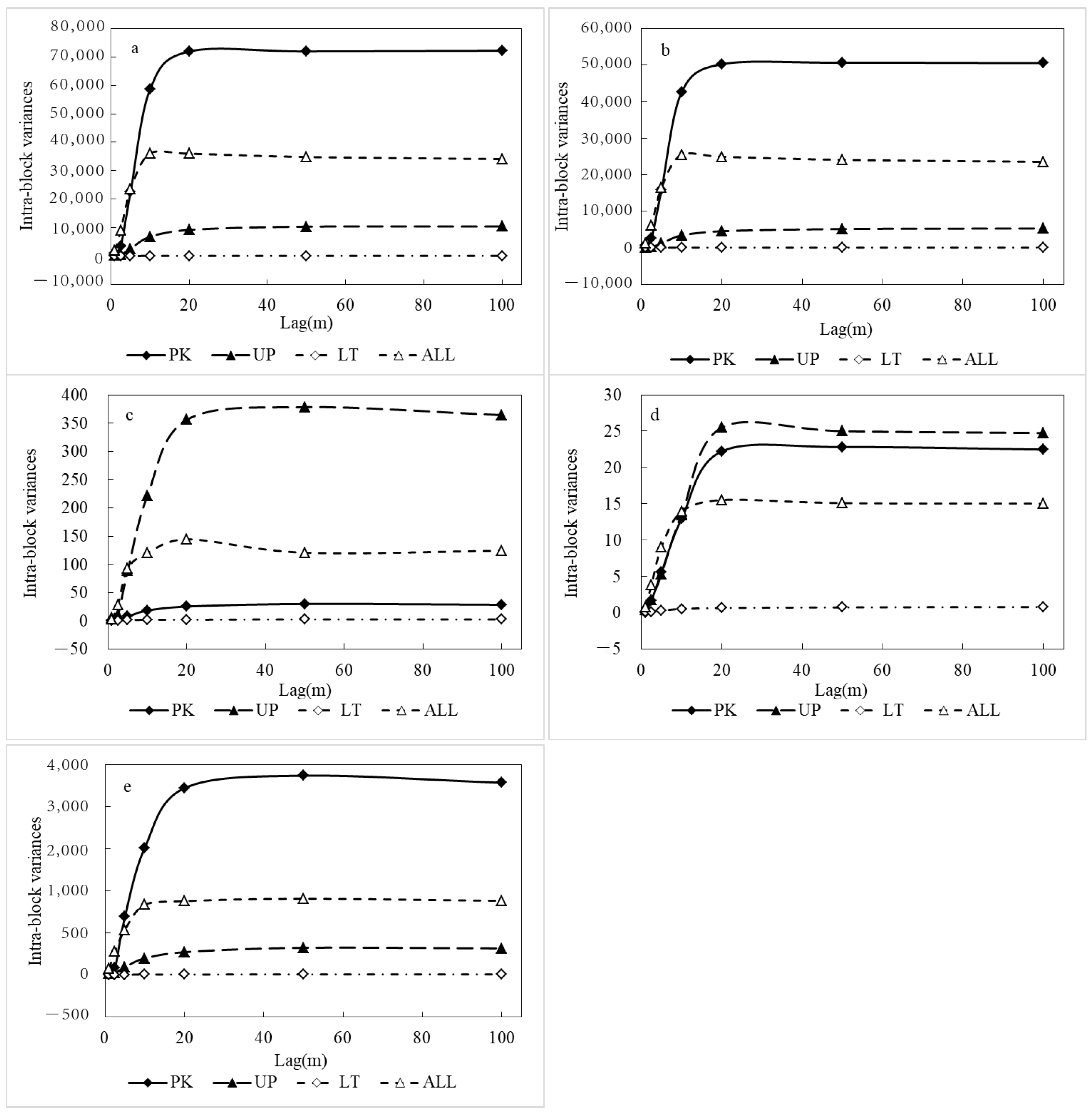
2.4.1. Spatial Heterogeneity of the Aboveground Biomass

The intra-group variance can be used to describe the spatial heterogeneity of study subjects quantitatively. This is a function of block size and usually increases as the size of the blocks increases [73], and it can be calculated by Equation (1).
S intra = 1 B g = 1 B 1 n g h = 1 n g ( X g h X ¯ g ) 2
where B is the number of groups at a particular grouping distance; Xgh is the h-th observation biomass value in the g-th block; X g is the mean of observation value in the g-th block.

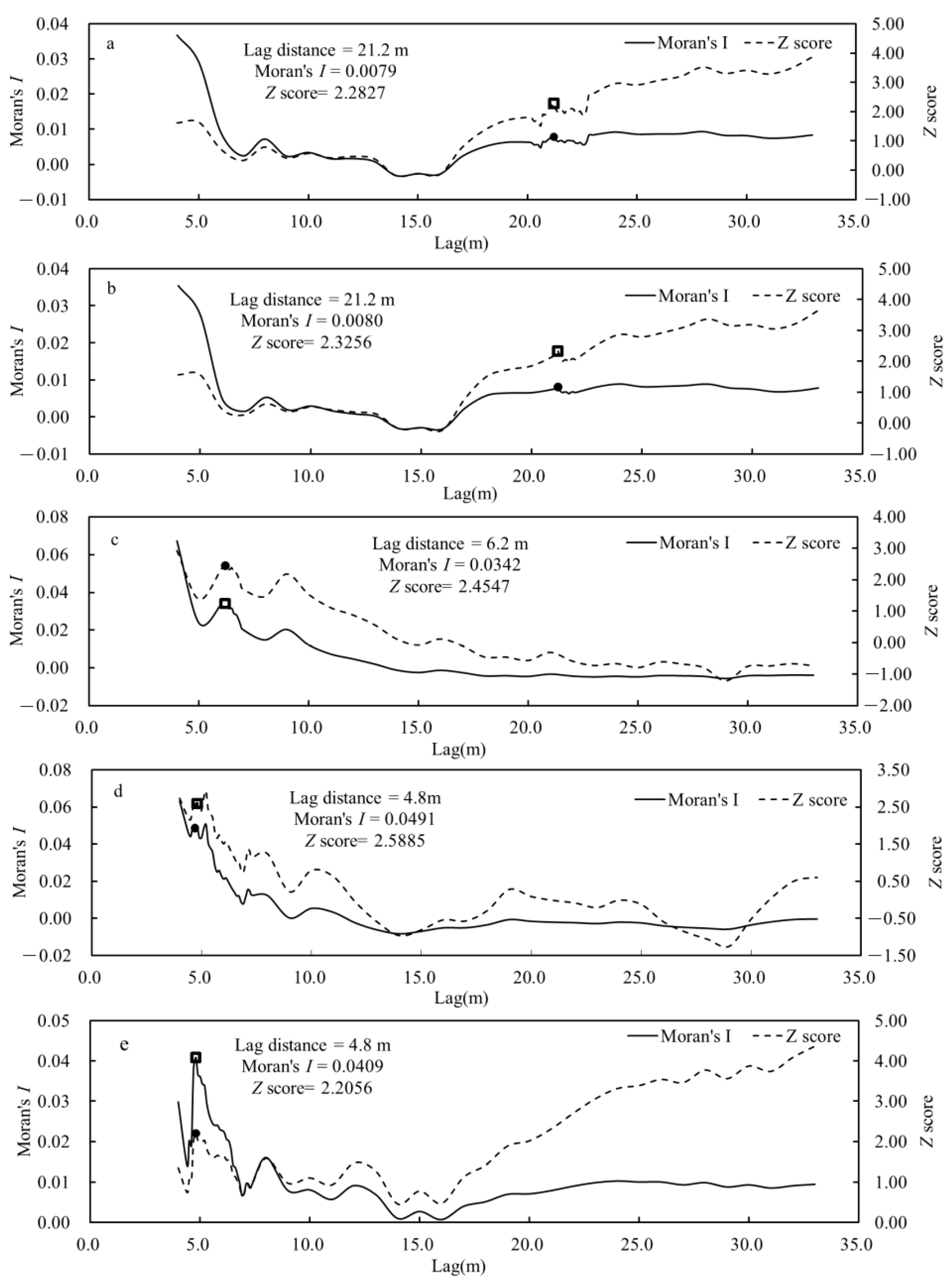
2.4.2. Spatial Autocorrelation of the Aboveground Biomass

Moran’s I effectively reflect the differences and correlations in the spatial distribution of observations. It can also reflect the overall spatial clustering pattern of objects in the study area [11]. The value range of Moran’s I is between (−1, 1). The closer the absolute value of the index value is to 1, the greater the degree of aggregation. When Moran’s I is positive, the observations within the distance (h) tend to be similar.
On the contrary, they tend to be dissimilar when the coefficient is negative. If Moran’s I index is close to or equal to 0, the observations are spatially random and independent. So, Moran’s I was chosen to describe the spatial autocorrelation for each component biomass (Equation (2)).
I = ( n i = 1 n j = 1 n w i j ( d ) ) i = 1 n j = 1 n w i j ( d ) ( x i x ¯ ) ( x j x ¯ ) i = 1 n ( x i x ¯ ) 2
where n is the number of plots; xi and xj are the observation value at plot i and plot j, x ¯ is the average of all attribute values; w i j ( d ) is the spatial weight matrix value that represents the relationship between plot i and plot j of the spatial object.
After the Moran index value is calculated, the significance of the index is tested by a Z-score. The higher (or lower) the Z-score, the higher the degree of clustering. A positive Z-score indicates a cluster of high values, and a negative Z-score indicates clusters of low values. If the Z-score is close to zero, no significant clustering exists within this area, and the Z-score was calculated by Equation (3).
Z ( I ) = I E ( I ) V a r ( I ) , E ( I ) = 1 n 1
where Z(I) is an index to measure the strength of spatial clustering patterns; E(I) and Var(I) are the expected value and variance of the index value I, respectively;
Moreover, local spatial autocorrelation can be used to describe the degree of spatial correlation between a research object and its adjacent units. In this study, the distance corresponding to the first peak after each component’s spatial clustering pattern for biomass reached significance was used as the bandwidth, and ArcGIS was used to calculate local Moran’s Ii. Furthermore, the local Moran’s Ii was calculated by Equation (4):
I i = n 2 i n j n w i j ( x i x ¯ ) j n w i j ( x j x ¯ ) i n ( x i x ¯ ) 2
where n is the number of plots; xi and xj are the observation value at plot i and plot j, x is the average of all attribute values; w i j ( d ) is the spatial weight matrix value. Different from the global Moran’s I, the value range of the local Moran’s Ii is not limited to (−1, 1); if the Ii value is positive, it shows that the location of the plot is a positive correlation and reflects the aggregation of similar values. But the Ii is negative, and it shows that the location of the plot is a negative correlation and reflects the aggregation of different values.
The global Moran’s I and Z (I) values were calculated using the incremental spatial autocorrelation tool in ArcGIS. The most significant distance of the spatial clustering pattern obtained from the incremental spatial autocorrelation analysis was used as the scale parameter for local spatial autocorrelation analysis. On this basis, using ArcGIS clustering and outlier analysis tools, the spatial weight matrix was constructed in the form of fixed distance bandwidth, and the local Moran’s Ii was calculated to quantitatively describe the spatial correlation between local, regional observations.

3. Results

3.1. Spatial Heterogeneity of the Aboveground Biomass

The spatial heterogeneity variation in biomass of each component showed the same trend in the range of 0–100 m (Figure 3). Aboveground, wood, branches, bark, and foliage were the order of the intra-group variance values for the different components. Although the value changed with the different organs, the spatial variation gradually increased with increasing distance; after reaching a certain distance, the variation tended to be stable. The variance values tended to be stable after 20 m for both PK and UP. In comparison, the variation of LT and all tree species tended to be stable after 10 m. Furthermore, the spatial variance values of PK were significantly larger than the other tree types for the AGB, wood, and branches. The spatial variance values of UP were the largest for both bark and foliage, and all the biomass components of the LT showed the smallest spatial variance values.

3.2. Spatial Autocorrelation of the Aboveground Biomass

3.2.1. Global Moran’s I

The global Moran’s I of each component biomass at the different lag distances were calculated, and the Moran’s I correlogram and Z-score values of the biomass with lag distances are shown, respectively. For all trees (Figure 4), the distances at the first peak (DFP) with a significant Z-score larger than 1.96 were 21.2 m for the AGB and wood biomass. The distance value was 6.2 m, and the biomass for both the foliage and branch was 4.8 m. Moreover, at the corresponding lag distance, the spatial autocorrelation was significant because the Z-scores were larger than 1.96. Meanwhile, the Moran’s I values of AGB and wood were lower than 0.01, and the values of foliage, bark, and branches were larger than 0.034.
For the different tree types, the PK had a similar change law for all trees; the DFP was 12.4 m for both AGB and wood biomass, 10.0 m for bark biomass, and 7.4 m for both foliage and branches. Furthermore, the Moran’s I was larger than 0.13 for foliage and branches; the values for the AGB, wood, and bark were 0.0687, 0.0609, and 0.0389, respectively (Figure 5). For the UP, the spatial autocorrelation of both foliage and branches was not significant because the Z score was not significant along with the lag distance, and the absolute Z scores were not larger than 1.96. Meanwhile, the DFP of AGB, wood, and bark were 6.6 m, 6.6 m, and 9.0 m, respectively. The corresponding Moran’s I values were 0.1277, 0.1372, and 0.1644 (Figure 6). Moreover, for LT, the branch biomass had no significant spatial autocorrelation, and the Moran’s I of both AGB and wood were 0.0520 and 0.0617 at a DFP of 6.4 m. The bark biomass had the largest DFP at 17.5 m, and the Moran’s I was 0.0233. Meanwhile, the foliage biomass had the lowest DFP at 6.0 m, and the Moran’s I was 0.0771 (Figure 7).
Moreover, we can find that the AGB and wood biomass had the same DFP for each tree type for all trees. Additionally, they had the highest DFP for all trees and PK but the lowest UP, and most of the foliage biomass had a lower DFP, with the largest Moran’s I for each tree type and all trees. Furthermore, a large portion of the PK and UP had the highest Moran’s I when compared to that of LT.

3.2.2. Local Moran’s Ii

The counting statistics of spatial autocorrelation were made and listed in Table 3. The PK had a lower percentage of the point with no significant spatial autocorrelation (NS) when compared with UP and LT. Especially for the LT, the percentage of the NS point was greater than 98%, and all points were the NS for the wood biomass and AGB. But for the PK, the percentage with NS for the wood biomass and AGB were the lowest, and the percentage was 77.27% and 78.03%, respectively. Moreover, for the point with significant spatial autocorrelation, there was no similar aggregation point for low-low clustering (LL) for all trees; there were similar aggregation points for high-high clustering (HH), and a dissimilarity aggregation point for high-low outliers (HLs) were not found in the LT. The point with significant spatial autocorrelation in the plot was primarily LH outliers and HH clustering, and wood and AGB showed similar local spatial autocorrelation. HH points were mainly found in the wood, foliage, and AGB of PK, and bark biomass of UP. Meanwhile, HL points were mainly found in the wood and AGB of PK. For the dissimilarity aggregation points with a low-high outlier (LH), the percentage was lower; all UP was not found at the point with LH, and only 1 point for branches biomass for PK was found for LH.
Moreover, the spatial autocorrelation for each biomass component of the different tree or tree groups was shown in the local Moran’s Ii scatters. For the PK, the biomass of AGB, wood, and branches mainly showed significant HH clustering on the right side of the plot, while the spatial clustering pattern of biomass in the middle and left sides showed HL outliers. In addition, the biomass of bark and foliage mainly showed HH clustering within the plots. The biomass of some components was also accompanied by the LH outlier (Figure 8). For the UP, AGB and wood biomass showed HH clustering on the right side of the plot and NS on the left side. Similarly, foliage biomass also showed HH clustering on the right side of the plot, but an HL outlier was also present on the right and left sides. In contrast, bark biomass showed mainly HH clustering in the plot; HL outliers were found on the right center and near the left edge of the plot (Figure 9). But for the LT, the components mainly showed no significant aggregation (NS) and sporadic LH outliers in the plot (Figure 10).
Furthermore, for different tree species and components, we calculated the local Moran’s Ii of each tree using all trees. The statistics are listed in Table 4. According to the local autocorrelation analysis of biomass in different tree species and different components, it can be seen that, for the mean local autocorrelation value of wood biomass, the autocorrelation coefficient of PK showed a negative value, and the value (−0.45) was smaller than other trees (upper trees, lower trees, and total), with a negative autocorrelation. The minimum value (−10.32) and maximum value (8.43) were consistent with the total, and the minimum value was smaller than the other upper and lower trees, while the maximum value was larger than them. However, the standard error (0.23) was the largest among all tree species. For the local autocorrelation analysis of bark biomass, it can be seen that all tree species showed a positive correlation, and the highest mean correlation value (0.82) was found in other upper trees, and the highest value (20.07) was the same as that of the total. For the mean autocorrelation of foliage and branches biomass, except for the negative correlation of other upper trees, all showed a positive correlation, and the correlation of PK was the strongest; for foliage (0.39) and branches (0.17), the maximum value was the same as the total: foliage (12.73) and branches (14.35) and was higher than the other upper and lower trees. The mean, maximum, and minimum values of the local autocorrelation coefficients of AGB exhibited the same trend as wood biomass.

4. Discussion

4.1. Spatial Heterogeneity and Autocorrelation in the Tropical Natural Forest

The forest community has high spatial heterogeneity [74]. Under heterogeneous conditions, community differentiation led to self-thinning, weakened inter-specific competition, and enhanced individual stress resistance, which was beneficial for the stability of various groups in the community and the overall development of the community. In this study, in the range of 0–100 m, the change in spatial heterogeneity tended to be stable after a distance of 20 m. The spatial distribution of wood, bark, branches, foliage, and AGB in the natural forests of Pinus kesiya var. langbianensiss was not random but was positively correlated and showed some spatial aggregation. The semi-variance model structure could indicate the spatial heterogeneity of AGB [75]. As the distance increases, the correlation between the spatial variables and their surrounding values decreases [62], and this pattern was similar to the biomass in the broadleaved forests [76].
Moreover, the high biomass values were mainly concentrated on the right side of the sample plot, and the low values were mainly concentrated on the left and middle of the sample plot. The spatial clustering characteristics objectively existed in all biomass components [77]. Local spatial correlations were more robust for aboveground, wood, and bark biomass and mostly showed high-high aggregation and high-low outliers, with the lowest correlations for branch biomass. In addition, the findings indicated that the local spatial autocorrelation of the biomass components of lower tree species was more significant compared to that of other tree species. It could cause spatial patches within the stand by the specific dynamic processes that vary by spatial correlations among the tree species and local disturbances [64] and lead to spatial heterogeneity in the stand structure as well as within and among the tree species [78,79]. Therefore, it may be responsible for the spatial effects on individual tree biomass. Based on this, it can guide the study of the spatial structure, spatial heterogeneity, spatial autocorrelation, and biomass of Pinus kesiya var. langbianensiss natural forest in large regions. Rödig et al. [80] demonstrated how this linkage allowed for quantifying the spatial variation in forest structure caused by tree-level to regional-scale disturbances. In addition, the study of heterogeneity can also combine with remote sensing methods. Han et al. [81] estimated and explored the aboveground carbon storage (AGC) of bamboo forests by using Landsat images and five dates measured in the field. The results showed that the AGC of the moso bamboo increased gradually in the five periods, and its spatial heterogeneity had moderate autocorrelation.
The results of this study show that the AGB and the biomass of each component have spatial heterogeneity and spatial autocorrelation, which can be estimated by considering spatial regression models, such as GWR, in future studies. The GWR model has performed well in estimating biomass in many studies [51,52,53,61]. However, when estimating biomass or other tree characteristics, the applicability of the model needs to be fully considered before it can be calculated. The use of the SEM model enables a direct explanation of spatial autocorrelation. Meanwhile, the incorporation of spatial dependencies and variability in the modeling process through LMM (linear mixed model) and GWR techniques allows for improved data fitting and a more precise prediction of response variables [61].

4.2. Spatial Effect of the Different Components

The following results were obtained from the study of spatial heterogeneity regarding the biomass of different components. The components, which were ranked in terms of intra-group variance values, were aboveground, wood, branches, bark, and foliage, respectively. There was an allometric relationship for plant growth, and the plants preferentially allocated biomass to organ harvesting according to the biomass allocation theory [82]. Moreover, biomass allocation may vary with stand age, species competition, etc. [83], and therefore affect the spatial effect in the different components of biomass. Competition may have an especially meaningful impact on the biomass allocation of trees. Plant competition and herbivory interactions were crucial for reducing plant production performance and changing biomass allocation patterns [84]. The biomass allocation would prefer tree crowns with little light and tree roots with limited nutrients or water [82]. Under different light environments, there was no difference in the biomass allocation of stems and roots and leaf mass per area between invasive and native species [85]. In this study, the AGB had a much more significant spatial variation in the whole stand. This was consistent with the results of Du et al. [75] research on spatial heterogeneity and the carbon contribution of AGB of moso bamboo in Anji County, Zhejiang Province; in addition, their research also indicated that spatial autocorrelation had a determinative influence on the spatial heterogeneity and spatial distribution pattern of moso bamboo’s AGC. Therefore, the study of biomass cannot ignore the impact of spatial heterogeneity and spatial autocorrelation.
In addition, it is important to carry out a spatial autocorrelation analysis of the biomass of each component. In this study, global and local spatial autocorrelation analyses were carried out for the different components of different tree species so that the spatial autocorrelation between trees in the whole stand could be more easily seen. The global spatial autocorrelation trends for each component of Pinus kesiya var. langbianensis were consistent with those of all trees in the sample plot, while the trends for other upper trees and other lower trees differed from those of all trees in the sample plot. Zhou et al. [83] conducted biomass modeling of the moso bamboo foliage as a way to accurately estimate the dynamics of foliage biomass, thus contributing to the development of accurate simulations. The spatial autocorrelation was used by Wu et al. [86] to conduct a spatio-temporal analysis of forest stock in Sichuan Province, and a mapping exercise was conducted for global spatial autocorrelation and local spatial autocorrelation.
The local spatial autocorrelation of biomass is also essential, as the distribution of habitat factors, such as light, water, and soil, are heterogeneous in natural environments [87]. Stand volume and biomass are closely related, as habitat variation can lead to the territorial and specific structural characteristics of forest volume [88]. The local spatial autocorrelation analysis revealed distinct patterns of aggregation in the sample plots for the different components studied. Specifically, the HH, HL, and LH aggregations exhibited varying location and aggregation patterns. Stand volume was a stochastic function that related to random variables and location [86]; therefore, forest biomass estimation needs to take full account of the spatial location and distribution of trees. Spatial autocorrelation to interpret and aid model outputs can identify areas that are systematically sensitive to specific model inputs and can also guide the collection of additional data to refine model predictions [89].

4.3. Spatial Effect of the Different Tree Species

The spatial variance values of PK were significantly larger than the other tree types for the aboveground, wood, and branches biomass. The spatial variance values of UP were the largest for both bark and foliage, and the biomass components of the LT showed the smallest spatial variance values. Then, significant or highly significant spatial autocorrelations were found for the biomass of all the components except for the branches of LT and the foliage and branches for UP. The results showed that there was similar aggregation (high-high clustering or low-low clustering) or dissimilarity aggregation (high-low outlier or low-high outlier) regarding biomass in the natural stand of Pinus kesiya var. langbianensis but the correlation was not strong. Therefore, the spatial autocorrelation variation patterns of AGB and wood biomass were similar, and the patterns of foliage and branches biomass were comparatively similar (Figure 4, Figure 5, Figure 6 and Figure 7).
The species characteristics and specific dynamic process make the biomass allocation among the tree species different [64]; this then leads to the forest structure and spatial heterogeneity of different components and various tree species [78,79], which may be the reasons that affect the spatial effect of individual tree biomass. In this study, the stand was dominated by the masculine species of Pinus kesiya var. Langbianensis. Pinus kesiya var. Langbianensis is a typical fast-growing heliophilous species; the spatial autocorrelation of Pinus kesiya var. langbianensis natural forest was dominated by positive spatial autocorrelation for each component’s biomass, and there was significant positive spatial autocorrelation. Therefore, the spatial correlation was more prominent in Pinus kesiya var. langbianensis in terms of different tree species.
Moreover, the local spatial autocorrelation of each biomass component for the lower tree species was stronger than that of other tree species. The foliage biomass of the lower trees and all trees, the bark biomass of other upper trees, and the branches biomass of Pinus kesiya var. langbianensis were strongly correlated. However, it was also found that the biomass of some components had insignificant spatial autocorrelation, such as the foliage biomass of the upper tree species and the foliage biomass of the lower tree species. Subsequently, competition may be one of the main reasons.
The competition strongly affected tree productivity and reproductive capacity [84,85]. Light is one of the most critical factors controlling tree survival and growth, and the canopy formed by the upper layer of trees can limit the use of light resources by the species in the lower layer [90]. When compared to the dominant and upper-layer species, the lower-layer species had the most negligible spatial variation in the biomass of each component. The upper tree species allocated more of the obtained resources to the physiological activities of the foliage [47,61], coupled with the photosynthetic capacity of the bark being more sensitive to temperature [91]. The foliage and bark in the upper tree species got more light compared to the other types, and competition was more pronounced.

4.4. The Limits of the Study

The clear-cutting sample plot of Pinus kesiya var. langbianensis natural forest is 0.3 hectares; this study carried out spatial effect analysis on the data by calculating the variance of each component biomass and Moran’s index. It concluded that there was spatial heterogeneity in the biomass of an individual tree within a certain distance. This study explored spatial autocorrelation and spatial heterogeneity among individual trees. The study site is located in the main distribution area of Pinus kesiya var. langbianensis in Yunnan Province, namely the semi-humid areas of the northern tropical and southern subtropical regions of Yunnan Province. The stand structure is basically the same, with relatively small differences in site conditions and stand age [72]. Therefore, the sample plots were representative of the specific characteristics of the region. However, the number of sample plots could be increased in the next study; thus, spatial autocorrelation and spatial heterogeneity at the stand scale could be more easily investigated. Du et al. [75] investigated 55 sample plots with a sample size of 30 m × 30 m to study the spatial heterogeneity and spatial patterns of the above-ground biomass of moso bamboo. Meanwhile, the differences in physiological, biochemical characteristics, and stand structure between heliophilous species and shade-tolerant trees and the spatial effects of forest biomass dominated by other shade-tolerant species must be further studied.
Moreover, little research about the quantitative analysis of the spatial effects of individual tree AGB at a plot scale has been conducted because the measurement of biomass data is destructive and labor-intensive [80]. In this study, we discussed the reasons for the spatial effect of the natural forest of Pinus kesiya var. langbianensis. Moreover, only one sample plot was harvested using a clear-cutting plot; to some extent, it also reflects the organ and inter-specific differences of AGB at an individual tree scale for the Pinus kesiya var. langbianensis forest. However, there is a lack of validation or evidence from the relevant research. Therefore, in future research, the techniques employed in this study can be extended to investigate the spatial effects of biomass across a larger number of sample plots and more forest types to further confirm the spatial effect of the tree biomass in a forest at an individual tree scale. Additionally, the utilization of spatial regression models can be explored as a means to explore the spatial effect analysis for biomass.

5. Conclusions

In this study, all trees in a plot with 0.3 hectares (30 m × 100 m) for Pinus kesiya var. langbianensis natural forest were entirely cut down in Mojiang County, Yunnan Province, southwestern China. Then, the AGB of each tree was measured according to different organs, such as wood, bark, foliage, and branches. The intra-group variance was applied to describe the spatial heterogeneity of biomass in each component, and the global and local Moran indices were used to analyze the spatial autocorrelation for the three types of tree species, such as Pinus kesiya var. langbianensis (PK), the other upper trees (UPs), and the other lower trees (LTs). Therefore, these are the following conclusions.
(1) There was spatial heterogeneity for the biomass of each component in the P. kesiya var. langbianensis natural forest. The spatial heterogeneity of each biomass component showed an increase with distance and stabilization at distances of about 20 m for the UP and PK, but for the LT, the distance values were 10 m.
(2) The spatial autocorrelation differences among the organs were obvious, and some components showed a similar change trend. The spatial autocorrelation trend of AGB and wood biomass were similar, while bark biomass and foliage biomass had a similar spatial variation trend.
(3) The spatial effect was various for the different trees or tree groups. The weakest spatial heterogeneity was found in LT, while PK showed strong spatial heterogeneity in all components except bark biomass. PK and UP also showed significant spatial autocorrelation, with a global Moran’s I of 0.0389–0.1537 and 0.1277–0.1644, respectively.

Author Contributions

X.Z. and G.C. participated in the collection of field data, conducted data analysis, and wrote the draft of the paper; C.L., Q.F., W.L. and Y.W. participated in the collection of field data and data analysis; H.X. helped with data analysis and writing of the paper. G.O. supervised and coordinated the research project, designed the experiment, and revised the paper. All authors have read and agreed to the published version of the manuscript.

Funding

The study was financially supported by the National Natural Science Foundation of China (grant numbers 31560209 and 31760206), and the Ten-Thousand Talents Program of Yunnan Province, China (YNWR-QNBJ-2018-184).

Institutional Review Board Statement

Not applicable.

Informed Consent Statement

Not applicable.

Data Availability Statement

Not applicable.

Acknowledgments

The authors would like to thank the faculty and students at the College of Forestry, Southwest Forestry University (SWFU), China.

Conflicts of Interest

The authors declare that they have no competing financial interest or personal relationships that could have appeared to influence the work reported in this paper.

References

  1. Pretzsch, H. Trees grow modulated by the ecological memory of their past growth. Consequences for monitoring, modelling, and silvicultural treatment. For. Ecol. Manag. 2021, 487, 118982. [Google Scholar] [CrossRef]
  2. Bhandari, S.K.; Veneklaas, E.J.; McCaw, L.; Mazanec, R.; Whitford, K.; Renton, M. Individual tree growth in jarrah (Eucalyptus marginata) forest is explained by size and distance of neighbouring trees in thinned and non-thinned plots. For. Ecol. Manag. 2021, 494, 119364. [Google Scholar] [CrossRef]
  3. Aussenac, R.; Bergeron, Y.; Gravel, D.; Drobyshev, I. Interactions among trees: A key element in the stabilising effect of species diversity on forest growth. Funct. Ecol. 2019, 33, 360–367. [Google Scholar] [CrossRef]
  4. Anselin, L.; Griffith, D.A. Do spatial effecfs really matter in regression analysis? Pap. Reg. Sci. 1988, 65, 11–34. [Google Scholar] [CrossRef]
  5. Zhang, L.; Shi, H. Local modeling of tree growth by geographically weighted regression. For. Sci. 2004, 50, 225–244. [Google Scholar]
  6. Stojanova, D.; Ceci, M.; Appice, A.; Malerba, D.; Džeroski, S. Dealing with spatial autocorrelation when learning predictive clustering trees. Ecol. Inform. 2013, 13, 22–39. [Google Scholar] [CrossRef] [Green Version]
  7. Anselin, L. Lagrange multiplier test diagnostics for spatial dependence and spatial heterogeneity. Geogr. Anal. 1988, 20, 1–17. [Google Scholar] [CrossRef]
  8. Chen, Y. New approaches for calculating Moran’s index of spatial autocorrelation. PLoS ONE 2013, 8, e68336. [Google Scholar] [CrossRef] [Green Version]
  9. Legendre, P. Spatial autocorrelation: Trouble or new paradigm? Ecology 1993, 74, 1659–1673. [Google Scholar] [CrossRef]
  10. Kashlak, A.B.; Yuan, W. Computation-free nonparametric testing for local spatial association with application to the US and Canadian electorate. Spat. Stat. 2022, 48, 100617. [Google Scholar] [CrossRef]
  11. Moran, P.A. Notes on continuous stochastic phenomena. Biometrika 1950, 37, 17–23. [Google Scholar] [CrossRef] [PubMed]
  12. Geary, R.C. The contiguity ratio and statistical mapping. Inc. Stat. 1954, 5, 115–146. [Google Scholar] [CrossRef]
  13. Getis, A.; Ord, J.K. The analysis of spatial association by use of distance statistics. Geogr. Anal. 1992, 24, 189–206. [Google Scholar] [CrossRef]
  14. Darand, M.; Dostkamyan, M.; Rehmani, M. Spatial autocorrelation analysis of extreme precipitation in Iran. Russ. Meteorol. Hydrol. 2017, 42, 415–424. [Google Scholar] [CrossRef]
  15. Sari, F.; Frananda, H.; Fransiska, S. Identification of Spatial Autocorrelation in the Poverty Level in West Pasaman Regency with Moran Index. J. Phys. Conf. Ser. 2020, 1554, 012052. [Google Scholar] [CrossRef]
  16. Anselin, L. Local indicators of spatial association—LISA. Geogr. Anal. 1995, 27, 93–115. [Google Scholar] [CrossRef]
  17. Dalposso, G.H.; Uribe-Opazo, M.A.; Mercante, E.; Lamparelli, R.A. Spatial autocorrelation of NDVI and GVI indices derived from Landsat/TM images for soybean crops in the western of the state of Paraná in 2004/2005 crop season. Eng. Agrícola 2013, 33, 525–537. [Google Scholar] [CrossRef] [Green Version]
  18. Shi, H.; Zhang, L. Local analysis of tree competition and growth. Forest Sci. 2003, 49, 938–955. [Google Scholar]
  19. Chas-AMil, M.L.; PresTeMon, J.P.; MccleAn, C.J.; TouzA, J. Human-ignited wildfire patterns and responses to policy shifts. Appl. Geogr. 2015, 56, 164–176. [Google Scholar] [CrossRef]
  20. Anselin, L.; Kelejian, H.H. Testing for spatial error autocorrelation in the presence of endogenous regressors. Int. Reg. Sci. Rev. 1997, 20, 153–182. [Google Scholar] [CrossRef] [Green Version]
  21. Yin, C.; Yuan, M.; Lu, Y.; Huang, Y.; Liu, Y. Effects of urban form on the urban heat island effect based on spatial regression model. Sci. Total Environ. 2018, 634, 696–704. [Google Scholar] [CrossRef] [PubMed]
  22. Liu, Z.; Jiang, F.; Zhu, Y.; Li, F.; Jin, G. Spatial heterogeneity of leaf area index in a temperate old-growth forest: Spatial autocorrelation dominates over biotic and abiotic factors. Sci. Total Environ. 2018, 634, 287–295. [Google Scholar] [CrossRef] [PubMed]
  23. Junttila, V.; Laine, M. Bayesian Principal Component Regression model with spatial effects for forest inventory under small field sample size. arXiv 2016, arXiv:1605.07439. [Google Scholar] [CrossRef]
  24. Ferré, C.; Castrignanò, A.; Comolli, R. Comparison between spatial and non-spatial regression models for investigating tree–soil relationships in a polycyclic tree plantation of Northern Italy and implications for management. Agrofor. Syst. 2019, 93, 2181–2196. [Google Scholar] [CrossRef]
  25. Klooster, D.J. Toward adaptive community forest management: Integrating local forest knowledge with scientific forestry. Econ. Geogr. 2002, 78, 43–70. [Google Scholar] [CrossRef]
  26. Pickett, S.T.; Cadenasso, M.L. Landscape ecology: Spatial heterogeneity in ecological systems. Science 1995, 269, 331–334. [Google Scholar] [CrossRef]
  27. Carey, A. Biocomplexity and restoration of biodiversity in temperate coniferous forest: Inducing spatial heterogeneity with variable-density thinning. Forestry 2003, 76, 127–136. [Google Scholar] [CrossRef] [Green Version]
  28. Assal, T.J.; Anderson, P.J.; Sibold, J. Spatial and temporal trends of drought effects in a heterogeneous semi-arid forest ecosystem. For. Ecol. Manag. 2016, 365, 137–151. [Google Scholar] [CrossRef] [Green Version]
  29. Beckage, B.; Clark, J.S. Seedling survival and growth of three forest tree species: The role of spatial heterogeneity. Ecology 2003, 84, 1849–1861. [Google Scholar] [CrossRef]
  30. Ngao, J.; Epron, D.; Delpierre, N.; Bréda, N.; Granier, A.; Longdoz, B. Spatial variability of soil CO2 efflux linked to soil parameters and ecosystem characteristics in a temperate beech forest. Agric. For. Meteorol. 2012, 154, 136–146. [Google Scholar] [CrossRef]
  31. Ward, J.S.; Parker, G.R.; Ferrandino, F.J. Long-term spatial dynamics in an old-growth deciduous forest. For. Ecol. Manag. 1996, 83, 189–202. [Google Scholar] [CrossRef]
  32. Brazhnik, K.; Shugart, H. Model sensitivity to spatial resolution and explicit light representation for simulation of boreal forests in complex terrain. Ecol. Model. 2017, 352, 90–107. [Google Scholar] [CrossRef]
  33. Gundale, M.J.; Metlen, K.L.; Fiedler, C.E.; DeLuca, T.H. Nitrogen spatial heterogeneity influences diversity following restoration in a ponderosa pine forest, Montana. Ecol. Appl. 2006, 16, 479–489. [Google Scholar] [CrossRef] [PubMed] [Green Version]
  34. Gossner, M.M.; Getzin, S.; Lange, M.; Pašalić, E.; Türke, M.; Wiegand, K.; Weisser, W.W. The importance of heterogeneity revisited from a multiscale and multitaxa approach. Biol. Conserv. 2013, 166, 212–220. [Google Scholar] [CrossRef]
  35. Hewitt, J.E.; Thrush, S.F.; Dayton, P.K.; Bonsdorff, E. The effect of spatial and temporal heterogeneity on the design and analysis of empirical studies of scale-dependent systems. Am. Nat. 2007, 169, 398–408. [Google Scholar] [CrossRef]
  36. Detto, M.; Asner, G.P.; Muller-Landau, H.C.; Sonnentag, O. Spatial variability in tropical forest leaf area density from multireturn lidar and modeling. J. Geophys. Res. Biogeosci. 2015, 120, 294–309. [Google Scholar] [CrossRef]
  37. Getzin, S.; Fischer, R.; Knapp, N.; Huth, A. Using airborne LiDAR to assess spatial heterogeneity in forest structure on Mount Kilimanjaro. Landsc. Ecol. 2017, 32, 1881–1894. [Google Scholar] [CrossRef]
  38. Clark, P.J.; Evans, F.C. Distance to nearest neighbor as a measure of spatial relationships in populations. Ecology 1954, 35, 445–453. [Google Scholar] [CrossRef]
  39. Madden, L.; Hughes, G.; Ellis, M. Spatial heterogeneity of the incidence of grape downy mildew. Phytopathology 1995, 85, 269–275. [Google Scholar] [CrossRef]
  40. Perry, G.L.; Miller, B.P.; Enright, N.J. A comparison of methods for the statistical analysis of spatial point patterns in plant ecology. Plant Ecol. 2006, 187, 59–82. [Google Scholar] [CrossRef]
  41. Fotheringham, A.S. Trends in quantitative methods I: Stressing the local. Prog. Hum. Geogr. 1997, 21, 88–96. [Google Scholar] [CrossRef]
  42. Fotheringham, A.S. “The problem of spatial autocorrelation” and local spatial statistics. Geogr. Anal. 2009, 41, 398–403. [Google Scholar] [CrossRef]
  43. Yang, X.; Han, Y. Spatial heterogeneity of soil nitrogen in six natural secondary forests in mountainous region of northern China. Sci. Soil Water Conserv. 2010, 8, 95–102. [Google Scholar]
  44. Lamsal, S.; Rizzo, D.; Meentemeyer, R. Spatial variation and prediction of forest biomass in a heterogeneous landscape. J. For. Res. 2012, 23, 13–22. [Google Scholar] [CrossRef]
  45. Fotheringham, A.S.; Charlton, M.E.; Brunsdon, C. Geographically weighted regression: A natural evolution of the expansion method for spatial data analysis. Environ. Plan. A 1998, 30, 1905–1927. [Google Scholar] [CrossRef]
  46. Wang, Q.; Ni, J.; Tenhunen, J. Application of a geographically-weighted regression analysis to estimate net primary production of Chinese forest ecosystems. Glob. Ecol. Biogeogr. 2005, 14, 379–393. [Google Scholar] [CrossRef]
  47. Zhang, J.; Cheng, G.; Yu, F.; Kräuchi, N.; Li, M.-H. Interspecific variations in responses of Festuca rubra and Trifolium pratense to a severe clipping under environmental changes. Biologia 2009, 64, 292–298. [Google Scholar] [CrossRef]
  48. Nazeer, M.; Bilal, M. Evaluation of ordinary least square (OLS) and geographically weighted regression (GWR) for water quality monitoring: A case study for the estimation of salinity. J. Ocean. Univ. China 2018, 17, 305–310. [Google Scholar] [CrossRef]
  49. Pradhan, B.; Youssef, A.M. Manifestation of remote sensing data and GIS on landslide hazard analysis using spatial-based statistical models. Arab. J. Geosci. 2010, 3, 319–326. [Google Scholar] [CrossRef]
  50. Dale, M.R.; Fortin, M.-J. Spatial Analysis: A Guide for Ecologists; Cambridge University Press: Cambridge, UK, 2014. [Google Scholar]
  51. Zhang, B.; Ou, G.; Sun, X.; Xu, T.; Xu, H. Application of Spatial Effect and Regression Model on Forestry Research. J. Southwest For. Univ. 2016, 36, 144–152. [Google Scholar]
  52. Liu, C. Spatial Distribution of Forest Carbon Storage in Heilongjiang Province; Northeast Forestry University: Harbin, China, 2014. [Google Scholar]
  53. Zhou, L.; Ou, G.; Wang, J.; Xu, H. Light Saturation Point Determination and Biomass Remote Sensing Estimation of Pinus kesiya var. langbianensis Forest Based on Spatial Regression Models. Sci. Silvae Sin. 2020, 56, 38–47. [Google Scholar]
  54. Ou, G.L.; Wang, J.F.; Xiao, Y.F.; Xu, H. Modeling Individual Biomass of Pinus kesiya var.langbianensis Natural Forests by Geographically Weighted Regression. For. Res. 2014, 27, 213–218. [Google Scholar] [CrossRef]
  55. Ou, G.; Wang, J.; Xu, H.; Chen, K.; Zheng, H.; Zhang, B.; Sun, X.; Xu, T.; Xiao, Y. Incorporating topographic factors in nonlinear mixed-effects models for aboveground biomass of natural Simao pine in Yunnan, China. J. For. Res. 2016, 27, 119–131. [Google Scholar] [CrossRef]
  56. Lu, J.; Zhang, L. Evaluation of parameter estimation methods for fitting spatial regression models. For. Sci. 2010, 56, 505–514. [Google Scholar]
  57. Lu, J.; Zhang, L. Modeling and prediction of tree height–diameter relationships using spatial autoregressive models. For. Sci. 2011, 57, 252–264. [Google Scholar] [CrossRef]
  58. Lu, J.; Zhang, L. Geographically local linear mixed models for tree height-diameter relationship. For. Sci. 2012, 58, 75–84. [Google Scholar] [CrossRef]
  59. Gu, F.; Zhao, Q. Geographically weighted regression model for expressing tree growth relationships. J. Northeast For. Univ. 2012, 40, 129–140. [Google Scholar]
  60. Zhang, L.; Gove, J.H.; Heath, L.S. Spatial residual analysis of six modeling techniques. Ecol. Model. 2005, 186, 154–177. [Google Scholar] [CrossRef]
  61. Zhang, L.; Ma, Z.; Guo, L. An evaluation of spatial autocorrelation and heterogeneity in the residuals of six regression models. For. Sci. 2009, 55, 533–548. [Google Scholar]
  62. Meng, Q.; Cieszewski, C.J.; Strub, M.R.; Borders, B.E. Spatial regression modeling of tree height–diameter relationships. Can. J. For. Res. 2009, 39, 2283–2293. [Google Scholar] [CrossRef]
  63. Soto, D.P.; Salas, C.; Donoso, P.J.; Uteau, D. Structural and spatial heterogeneity of a mixed Nothofagus donibeyi-dominate forest stand after a partial disturbance. Rev. Chil. Hist. Nat. 2010, 83, 335–347. [Google Scholar]
  64. Rozas, V. Structural heterogeneity and tree spatial patterns in an old-growth deciduous lowland forest in Cantabria, northern Spain. Plant Ecol. 2006, 185, 57–72. [Google Scholar] [CrossRef]
  65. Pearce, H.; Anderson, W.; Fogarty, L.; Todoroki, C.; Anderson, S. Linear mixed-effects models for estimating biomass and fuel loads in shrublands. Can. J. For. Res. 2010, 40, 2015–2026. [Google Scholar] [CrossRef]
  66. Chai, Z. Quantitative Evaluation and R Programming of Forest Spatial Structure Based on the Relationship of Neighborhood Trees: A Case Study of Typical Secondary Forest in the Mid-Altitude Zone of the Qinling Mountains; Northwest A&F University: Yangling, China, 2016. [Google Scholar]
  67. Nong, M.; Leng, Y.; Xu, H.; Li, C.; Ou, G. Incorporating competition factors in a mixed-effect model with random effects of site quality for individual tree above-ground biomass growth of Pinus kesiya var. langbianensis. N. Z. J. For. Sci. 2019, 49. [Google Scholar] [CrossRef] [Green Version]
  68. Chen, Q.; Zheng, Z.; Feng, Z.; Ma, Y.; Sha, L.; Xu, H.; Nong, P.; Li, Z. Biomass and carbon storage of Pinus kesiya var. langbianensis in Puer, Yunnan. J. Yunnan Univ.-Nat. Sci. Ed. 2014, 36, 439–445. [Google Scholar]
  69. Fan, Y.; Zhang, S.; Lan, Z.; Lan, Q. Possible causes for the differentiation of Pinus yunnanensis and P. Kesiya var. Langbianensis in Yunnan, China: Evidence from seed germination. For. Ecol. Manag. 2021, 494, 119321. [Google Scholar]
  70. Flora of China Editorial Committee. Flora of China. 2018. Available online: http://www.efloras.org/flora_page.asp (accessed on 30 August 2018).
  71. Chen, G.; Zhang, X.; Liu, C.; Liu, C.; Xu, H.; Ou, G. Error Analysis on the Five Stand Biomass Growth Estimation Methods for a Sub-Alpine Natural Pine Forest in Yunnan, Southwestern China. Forests 2022, 13, 1637. [Google Scholar] [CrossRef]
  72. Nong, M. Comparative Analysis on the Spatial Effects of Individualtree Biomass in Typical Subtropical Forests; Southwest Forestry University: Kunming, China, 2020. [Google Scholar]
  73. Lieshout, M.v. AJ-function for marked point patterns. Ann. Inst. Stat. Math. 2006, 58, 235–259. [Google Scholar] [CrossRef]
  74. Turner, M.G.; Donato, D.C.; Romme, W.H. Consequences of spatial heterogeneity for ecosystem services in changing forest landscapes: Priorities for future research. Landsc. Ecol. 2013, 28, 1081–1097. [Google Scholar] [CrossRef]
  75. Du, H.; Zhou, G.; Fan, W.; Ge, H.; Xu, X.; Shi, Y.; Fan, W. Spatial heterogeneity and carbon contribution of aboveground biomass of moso bamboo by using geostatistical theory. Plant Ecol. 2010, 207, 131–139. [Google Scholar] [CrossRef]
  76. Wang, W.; Dong, X.; Dong, X.; Lv, D.; Su, T.; Zheng, A. Study on spatial autocorrelation of forest biomass. For. Eng. 2018, 34, 35–39. [Google Scholar]
  77. Liu, K.; Jiang, S.; Zhu, W. Estimation of carbon sequestration value and analysis of space effect of forests in Guangdong Province. Chin. J. Agric. Resour. Reg. Plan. 2015, 36, 120. [Google Scholar]
  78. Frelich, L.E.; Calcote, R.R.; Davis, M.B.; Pastor, J. Patch formation and maintenance in an old-growth hemlock-hardwood forest. Ecology 1993, 74, 513–527. [Google Scholar] [CrossRef]
  79. Park, A.; Kneeshaw, D.; Bergeron, Y.; Leduc, A. Spatial relationships and tree species associations across a 236-year boreal mixedwood chronosequence. Can. J. For. Res. 2005, 35, 750–761. [Google Scholar] [CrossRef] [Green Version]
  80. Rödig, E.; Cuntz, M.; Heinke, J.; Rammig, A.; Huth, A. Spatial heterogeneity of biomass and forest structure of the Amazon rain forest: Linking remote sensing, forest modelling and field inventory. Glob. Ecol. Biogeogr. 2017, 26, 1292–1302. [Google Scholar] [CrossRef]
  81. Han, N.; Du, H.; Zhou, G.; Xu, X.; Cui, R.; Gu, C. Spatiotemporal heterogeneity of Moso bamboo aboveground carbon storage with Landsat Thematic Mapper images: A case study from Anji County, China. Int. J. Remote Sens. 2013, 34, 4917–4932. [Google Scholar] [CrossRef]
  82. Xu, Q.; Li, B.; McRoberts, R.E.; Li, Z.; Hou, Z. Harnessing data assimilation and spatial autocorrelation for forest inventory. Remote Sens. Environ. 2023, 288, 113488. [Google Scholar] [CrossRef]
  83. Zhou, Z.; Tang, Y.; Xu, H.; Wang, J.; Hu, L.; Xu, X. Dynamic changes in leaf biomass and the modeling of individual Moso Bamboo (Phyllostachys edulis (Carrière) J. Houz) under intensive management. Forests 2022, 13, 693. [Google Scholar] [CrossRef]
  84. Nötzold, R.; Blossey, B.; Newton, E. The influence of below ground herbivory and plant competition on growth and biomass allocation of purple loosestrife. Oecologia 1997, 113, 82–93. [Google Scholar] [CrossRef]
  85. Pattison, R.; Goldstein, G.; Ares, A. Growth, biomass allocation and photosynthesis of invasive and native Hawaiian rainforest species. Oecologia 1998, 117, 449–459. [Google Scholar] [CrossRef]
  86. Wu, H.; Xu, H.; Tian, X.; Zhang, W.; Lu, C. Multistage Sampling and Optimization for Forest Volume Inventory Based on Spatial Autocorrelation Analysis. Forests 2023, 14, 250. [Google Scholar] [CrossRef]
  87. Wang, J.; Haining, R.; Cao, Z. Sample surveying to estimate the mean of a heterogeneous surface: Reducing the error variance through zoning. Int. J. Geogr. Inf. Sci. 2010, 24, 523–543. [Google Scholar] [CrossRef]
  88. Holmberg, H.; Lundevaller, E.H. A test for robust detection of residual spatial autocorrelation with application to mortality rates in Sweden. Spat. Stat. 2015, 14, 365–381. [Google Scholar] [CrossRef]
  89. Wulder, M.A.; White, J.C.; Coops, N.C.; Nelson, T.; Boots, B. Using local spatial autocorrelation to compare outputs from a forest growth model. Ecol. Model. 2007, 209, 264–276. [Google Scholar] [CrossRef]
  90. Bebre, I.; Annighöfer, P.; Ammer, C.; Seidel, D. Growth, morphology, and biomass allocation of recently planted seedlings of seven European tree species along a light gradient. iFor.-Biogeosci. For. 2020, 13, 261–269. [Google Scholar] [CrossRef]
  91. Ren, J.; Wang, H.; Wang, W.; Qu, D.; Wang, Q.; Zhong, Z. Responses of photosynthesis, chlorophyll fluorescence of poplar leaf and bark chlorenchyma to elevated temperature. Bull. Bot. Res. 2014, 34, 758–764. [Google Scholar]
Figure 1. Location of the clear-cutting plot. (a,b) shows the location of the plot in Mujiang county for Pu’er City, Yunnan Province, and (c) is a satellite image of the study site (Red frame); (d) shows the numbering of trees in the sample plot before logging, and (eg) the trees that were logged.
Forests 14 01177 g001
Figure 2. Location of the trees in the clear-cutting plot. PK is Pinus kesiya var. langbianensis, UP is the other trees at the upper layer, and LT is the other trees at the lower layer. The circle diameter is proportional to the tree DBH.
Forests 14 01177 g002
Figure 3. The intra-group variance of the different biomass components for different tree groups. (a): aboveground biomass, (b): wood biomass, (c): bark biomass, (d): foliage biomass, (e): branches biomass. PK is Pinus kesiya var. langbianensis, UP is the other trees at the upper layer, and LT is the other trees at the lower layer.
Forests 14 01177 g003
Figure 4. Moran’s I correlogram and Z-score values for the biomass of the different components for all trees. (a): aboveground biomass, (b): wood biomass, (c): bark biomass, (d): foliage biomass, and (e): branches biomass. The dots and rectangles represent the points of Moran’s I and Z-score at the first peak (DFP) with a significant Z-score, and the values were shown in the figure, respectively.
Forests 14 01177 g004
Figure 5. Moran’s I correlogram and Z-score values for the biomass of the different components for Pinus kesiya var. langbianensis. (a): aboveground biomass, (b): wood biomass, (c): bark biomass, (d): foliage biomass, and (e): branches biomass. The dots and rectangles represent the points of Moran’s I and Z-score at the first peak (DFP) with a significant Z-score, and the values were shown in the figure, respectively.
Forests 14 01177 g005
Figure 6. Moran’s I correlogram and Z-score values for the biomass of the different components of other upper trees. (a): aboveground biomass, (b): wood biomass, (c): bark biomass, (d): foliage biomass, and (e): branches biomass. The dots and rectangles represent the points of Moran’s I and Z-score at the first peak (DFP) with a significant Z-score, and the values were shown in the figure, respectively.
Forests 14 01177 g006
Figure 7. Moran’s I correlogram and Z-score values for the biomass of the different components of other lower trees. (a): aboveground biomass, (b): wood biomass, (c): bark biomass, (d): foliage biomass, and (e): branches biomass. The dots and rectangles represent the points of Moran’s I and Z-score at the first peak (DFP) with a significant Z-score, and the values were shown in the figure, respectively.
Forests 14 01177 g007
Figure 8. Spatial distribution of local Moran’s Ii for Pinus kesiya var. langbianensis (a) for aboveground biomass, (b) for wood biomass, (c) for bark biomass, (d) for foliage biomass, and (e) for branches biomass. NS is the point of no significant spatial autocorrelation, HH is the similar aggregation point with high-high clustering, HL is the dissimilarity aggregation point with a high-low outlier, and LH is the dissimilarity aggregation point with a low-high outlier.
Forests 14 01177 g008
Figure 9. Spatial distribution of local Moran’s Ii for other upper trees (a) for aboveground biomass, (b) wood biomass, (c) bark biomass, (d) foliage biomass, and (e) for branches biomass. NS is the point of no significant spatial autocorrelation, HH is the similar aggregation point with a high-high clustering, and HL is the dissimilarity aggregation point with a high-low outlier.
Forests 14 01177 g009
Figure 10. Spatial distribution of local Moran’s Ii for lower trees. The capital letters of the figure codes represent the different components (a) for aboveground biomass, (b) wood biomass, (c) bark biomass, (d) foliage biomass, and for (e) branches biomass. NS is the point of no significant spatial autocorrelation, and LH is the dissimilarity aggregation point with a low-high outlier.
Forests 14 01177 g010
Table 1. The basic characteristics of the clear-cutting plot.
LocationLatitudeLongitudeAltitude (m)Slope
Degree (°)
Aspect of Slope (°)
Yutang23°9′58.2″ N101°29′14.4″ E153022298
Table 2. The basic information of the sampling trees in the clear-cutting plot.
Trees or Trees GroupAge (Years)Height (m)DBH (cm)Biomass (kg)
WoodBarkBranchesFoliageAboveground
Pinus kesiya var. langbianensis (n = 132)Mean3717.0524.26236.446.7837.244.45284.91
Std. Err.104.589.93224.735.3347.834.74268.62
Min.166.807.003.290.140.510.064.07
Max.6625.6045.101075.7934.49307.2323.391180.42
Other upper trees (n = 119)Mean259.9714.7655.2415.1613.623.4587.47
Std. Err.104.217.7672.6119.0917.784.97102.08
Min.53.303.400.820.290.070.021.74
Max.4821.5036.00368.4988.85103.1731.70482.72
Other lower trees (n = 261)Mean166.366.735.971.321.770.549.60
Std. Err.51.662.626.811.552.740.8911.09
Min.52.204.000.830.070.030.001.22
Max.3512.0021.0044.2010.5721.047.6771.80
Total (n = 512)Mean249.9513.1276.845.9513.672.2298.68
Std. Err.125.539.81153.3111.1429.713.88184.67
Min.52.203.400.820.070.030.001.22
Max.6625.6045.101075.7988.85307.2331.701180.42
Table 3. Spatial distribution by Z-score using all trees. PK is Pinus kesiya var. langbianensis, UP is the other trees at the upper layer, and LT represents the other trees at the lower layer. NS is the point with no significant spatial autocorrelation, HH is the similar aggregation point with high-high clustering, LL is the similar aggregation point with low-low clustering, HL is the dissimilarity aggregation point with a high-low outlier, and LH is the dissimilarity aggregation point with a low-high outlier. N is the number of degrees of distribution for each component, and P is the proportion of distribution of each component.
Tree TypesComponentsNSHHHLLHLL
NP (%)NP (%)NP (%)NP (%)NP (%)
PKWood10277.27118.331914.3900.0000.00
Bark12896.9743.0300.0000.0000.00
Branches11889.3986.0653.7910.7600.00
Foliage11687.881511.3610.7600.0000.00
Aboveground10378.03129.091712.8800.0000.00
UPWood11798.3221.6800.0000.0000.00
Bark9983.191512.6154.2000.0000.00
Branches119100.0000.0000.0000.0000.00
Foliage11596.6410.8432.5200.0000.00
Aboveground11798.3221.6800.0000.0000.00
LTWood261100.0000.0000.0000.0000.00
Bark25898.8500.0000.0031.1500.00
Branches25999.2300.0000.0020.7700.00
Foliage26099.6200.0000.0010.3800.00
Aboveground261100.0000.0000.0000.0000.00
ALLWood48093.75132.54193.7100.0000.00
Bark48594.73193.7150.9830.5900.00
Branches49696.8881.5650.9830.5900.00
Foliage49195.90163.1340.7810.2000.00
Aboveground48193.95142.73173.3200.0000.00
Table 4. Local Moran’s Ii for the biomass of the different components.
Tree SpeciesIndicesWoodBarkFoliageBranchesAboveground
Pinus kesiya
var.
langbianensis
Mean−0.450.100.390.17−0.42
Std. Err.0.230.070.200.210.23
Skewness0.012.522.873.25−0.03
Kurtosis2.7213.5911.8315.042.18
Min.−10.32−2.06−3.87−4.58−9.67
Max.8.434.9412.7314.358.12
Other upper treesMean0.150.82−0.07−0.040.07
Std. Err.0.090.310.110.060.10
Skewness1.783.810.16−2.420.50
Kurtosis12.7217.689.8710.134.56
Min.−3.02−3.71−6.06−3.76−3.06
Max.6.4920.076.141.265.40
Other lower treesMean0.260.080.090.110.28
Std. Err.0.050.050.050.040.05
Skewness−0.72−2.05−2.59−4.19−0.86
Kurtosis0.187.4611.1228.110.79
Min.−2.60−4.64−4.23−5.00−3.24
Max.1.531.251.441.001.70
TotalMean0.050.260.130.090.05
Std. Err.0.070.080.060.060.07
Skewness−0.566.643.154.67−0.63
Kurtosis9.7664.7226.5646.347.90
Min.−10.32−4.64−6.06−5.00−9.67
Max.8.4320.0712.7314.358.12
Disclaimer/Publisher’s Note: The statements, opinions and data contained in all publications are solely those of the individual author(s) and contributor(s) and not of MDPI and/or the editor(s). MDPI and/or the editor(s) disclaim responsibility for any injury to people or property resulting from any ideas, methods, instructions or products referred to in the content.

