
Forest Land Expectation Value or Maximum Sustained Yield? Resolving A Long-Standing Paradox
National Council for Air and Stream Improvement, Inc., 1258 Windemere Ave, Naperville, IL 60564, USA
Forests 2023, 14(5), 1052; https://doi.org/10.3390/f14051052
Submission received: 16 February 2023
/
Revised: 13 May 2023
/
Accepted: 15 May 2023
/
Published: 19 May 2023
(This article belongs to the Section Forest Economics, Policy, and Social Science)
Abstract
:The Faustmann formula, equivalent to the land expectation value (LEV), yields the present value, starting with bare land, of an infinite series of future timber rotations for a stand. If this formula is used to find the rotation age that maximizes the present value, a lower annual harvest will result when compared to a maximum sustained yield (MSY) regime for an ownership with many stands. However, the LEV is strongly preferred by economists. This is the LEV vs. rents paradox. Herein, this paper demonstrates that an infinite series of annual harvests for an ownership under an even flow regime, discounted to the present using any interest rate, will provide the same optimal rotation age as the time of the peak MAI for a single stand, though with different estimates for the profitability, depending on the interest rate. Thus, rotations producing the MSY and the maximum financial return are identical when analyzed at the ownership scale but are not the same when based on the analysis at the stand scale using the Faustmann formula (LEV). This is the solution to the paradox. The formulas for internal rate of return (IRR) and the land valuation for transaction purposes are also presented.
1. Introduction
The peak mean annual increment (MAI), or maximum sustained yield (MSY), is a common target for determining the rotation age in planted, commercial forests [1,2]. An alternative determination of the rotation age, and therefore the harvest level, is the discounted revenue (present value, PV) for a stand starting with bare ground. For an infinite series of rotations for a single stand, the Faustmann formula (equivalent to the land expectation value, LEV) is recommended [3]. These two approaches yield very different timber rotation ages and harvest volumes. The recent literature characterizes the conflicting views as a rents or steady income (maximum sustained yield, MSY) framework vs. maximizing financial value [4,5,6]. The conflict can also be characterized between the ownership level and stand level analyses [7]. Many economic analyses evaluate management based on a single stand (e.g., [4,8,9]) without comparing the results from a rents approach. In fact, the LEV has been claimed to apply to a regulated forest for determining the rotation age (e.g., [4,5,10,11]). Note that these authors assert that it is not just a matter of preference but is a proven best solution. Helmedag [2] noted that the LEV is the dominant framework in the forest economics community. On the other hand, he also showed that landowners often use the MSY to determine the rotation age. Conversations by the author with staff at multiple US forest product companies revealed that both approaches are used by different companies. How could such disagreement continue for so long? The paradox of these two approaches is that both approaches claim to be objectively correct and optimal yet produce very different rotation ages and property-level harvest volumes. The LEV approach is clearly optimal for a single stand in a bare ground state, yet, when applied to an ownership of many stands, it produces a lower income per year [2,12,13]. In brief, the rotation resulting from considering bare land as the starting condition forces an uneconomic acceleration of the time of the harvest to minimize the depreciation of the income (or cost of borrowed funds). A rents framework does not present this problem.
Here, this paper presents a formulation for the present value (PV) for a regulated forest to help resolve this contradiction. Additionally, a distinction is made between business capital (the land base) and income, with the derivation of the IRR and land value metrics. The analysis is based on an analytic stand growth model for simplicity and clarity of exposition as well as modeled and empirical growth and yield data from intensively managed loblolly (Pinus taeda) pine stands in Georgia, North Carolina and Virginia.
1.1. Stand Growth
A popular growth model is the Weibull function [3], shown in Equation (1).
where a defines the asymptote for a defined area, b and c are the shape parameters and t is the number of years (Figure 1). This formula models the biomass (or other metrics such as roundwood) in kg/ha vs. time. The total wood mass could represent whole-tree chipping and the total stem mass could correspond to the harvest of multiple wood products. The Weibull function has certain advantages for fitting data compared to other monotonic growth functions, such as the Gompertz or logistic functions. The MAI value (Figure 1b) at t is simply f from Equation (1) divided by t. A simple numerical search of the MAI values provides the age T of the peak MAI, which is the optimal rotation for the MSY. Several factors can modify the conclusion that the peak MAI is optimal. If older trees become progressively more valuable due to, for example, more knot-free wood for high quality lumber or veneer, then the optimal rotation age will increase. Conversely, if older stands tend to have a deteriorating quality (e.g., heart rot, staining, mortality), then the time of the optimal harvest is more immediate. These factors can be accommodated by including an age-dependent wood price, as shown in the empirical examples below, or by discounting the yield for damage risk.
1.2. The Faustmann Model
A classic approach for determining the optimal rotation is to treat a stand as an investment. In this case, a discount rate in a present value (PV) calculation of a future harvest for a single ha at time T can be applied.
where r is the interest rate, c is the planting cost per ha (assumed to occur during a harvest after the initial period), is the yield per ha at the rotation age and v is the value per unit of wood sold (v = 1 means only the wood volume is considered). Typically, r is defined as the minimum interest rate a landowner will accept or a goal rate. It can also be viewed as the cost of money encumbered in the land investment. More properly, an infinite series of harvests of rotation length T using the Faustmann formula can be evaluated to find the LEV on a single ha basis.
The initial planting is not discounted, and subsequent replanting is considered to take place at each harvest. This is also called the bare land value. The rotation length T that maximizes the LEV is then identified by solving this equation numerically for different T values. Intermediate treatments (e.g., fertilization, pre-commercial thinning) and harvests (e.g., commercial thinning, selection cuts) can be incorporated into this framework.
The Faustmann formula for the LEV can yield biologically implausible results. The rotation age based on Equation (3) is generally younger than the age of the peak MAI [12], notwithstanding the special case developed by Binkley [8]. As shown in Figure 2a, the maximum LEV is obtained at younger ages as the discount rate increases. Compared to a maximum MAI age of 89, a discount rate of even 8% provides a rotation age of approx. 20 years for this yield function. This rotation age gives a harvest only 10% of the peak MAI harvest at the stand scale or 62.5% of the ownership scale annual harvest under an even flow regime. The shorter rotation also increases the annual planting costs by 4.45 times due to more frequent harvests. The graph in Figure 2a shows that the rotation age approaches the age of the maximum MAI (89y) as the discount rate nears zero. However, the LEV at a zero discount rate is undefined in Equation (3). That is, the PV for a single rotation (2) with r = 0 yields a rotation age equivalent to the age of the maximum MAI (the forest rent rotation). However, the LEV in Equation (3) at r = 0 is an infinite sum since future harvests are not discounted, and it cannot be used to find the rotation age. For larger discount rates, the LEV decreases to very low levels since the age of the harvest is so low that the yields from (1) are trivial. These problems mean that this approach needs further analysis, despite its elegance. The rents framework can be suggested as an alternative.
1.3. Forest Rents
The alternative approach to the LEV is a rents formulation. The rotation age is based on the age of the peak MAI. An even flow regime implies a fully regulated forest (equal area in each age class), but this restriction is relaxed below. This is a MSY forest. Using the age of the maximum stand MAI, the forest-level annual harvest volume (H) for a regulated forest of homogeneous species and productivity is shown in Equation 4a.
and the income (I) is:
where fp is the wood volume per ha at the age of the peak MAI, A is the area of the entire ownership (ha), T is the rotation age (yr), v is the value per unit volume harvested (stumpage) and ć is the annual cost per ha (property tax, road maintenance, etc.). The middle term reflects the annual replanting cost (area A/T replanted/yr). Note that the planting costs c in a given year are not from the same stands as those harvested in that year. Instead, they are from all the stands harvested the previous year. Note that some forest types, such as many broadleaf species, can be regenerated naturally with no replanting cost. This also has implications for any assumption that planting costs accumulate interest charges until the harvest, with this being a driver for earlier harvests. The peak MAI provides the stand rotation age T that corresponds to the MSY for a forest [3,12]. This can be determined by a numerical search using Equation (4b) for different T values, allowing T to also affect the yield. For a forest with multiple species and productivity, this analysis can be conducted for each category (e.g., pine, hardwood, low vs. high site index). The MSY results in the maximization of the annual cash flow for a landowner with many stands. In a rent framework, the costs are treated as repeated annual expenses across the ownership or a class of land (such as all the parcels that will be thinned or fertilized). The planting costs are for all the stands replanted in a given year, not just a focal stand, as presented in the Faustmann formula, as well as the property tax of the ownership, road maintenance costs, etc. The other periodic costs, such as fertilization, can be added to Equation (4b). That is, the expenses are not capitalized. An infinite series of annual costs and income with and without a particular treatment can be compared to evaluate whether that treatment should be conducted.
The analogy with a classic rent situation is clear. For an owner of a commercial building that is to be rented, a quantity of invested money (the building) yields the annual income (rents). Annual or periodic repairs or maintenance are required, along with annual property tax. The owner must determine whether this cash flow provides an adequate return on investment. Using the income I from Equation (4b), the quantity I/B, where B is the basis (the value of all the tied-up capital) provides the interest rate yielded by the investment, which is equivalent to the imputed interest or IRR. It is also equivalent to the effective interest rate from an infinite term (non-depleting) annuity. Suppose this value is 5%. If the property owner can achieve >5% from other uses of their money, then this is not a good investment. In the same way, a commercial forest landowner invests capital and obtains an annual income from the ownership. A major difference is that buildings will eventually deteriorate and need replacement, whereas forest land does not. Note that for calculating the income-imputed interest or the return on investment, subtracting the interest on borrowed capital is double counting. Doing so would yield a net income figure rather than a rate of return to compare to the basis. Instead, the borrowed funds are part of the basis.
Some US institutional landowners use the peak MAI to determine the rotation length (S. Prisley, NCASI, pers. comm. July 2021). Hyytiäinen and Tahvonen [4] documented that forest rents were a common framework in Finland. On the other hand, it appears that interest rates do affect the rotation age for landowners growing long-lived, high value timber trees, such as Douglas firs (Pseudotsuga menziesii) or some hardwoods (E. Sucre, Weyerhaeuser Company, pers. comm. July 2022).
How do we value land that is a regulated forest in a rents context? Suppose that the ownership has A/T area available for harvest each year, where A is the area of the ownership divided into T units to implement an even flow, where T is the rotation age. The income each year is given by Equation (4b). If the discounted income for an infinite series of annual harvests is computed instead of periodic harvests, the PV is given by Equation (5).
This sum converges after a few hundred iterations. The exact formula is available for the sum shown in Equation (6).
Note that for continuous discounting in [6], instead of annual (discrete), Formula (6) is simply I/r. The discrete sum from Equation (6) is more in line with annual financial accounting and taxation. If we expand Equation (7) with Equation (4) for the optimal rotation age T, the following equation can be obtained.
which follows the definition of the value for a business. The Fisherian value of capital is defined as the discounted present value of the future income stream [15]. The rotation age in Equation (7) is not affected by discounting since the net annual income is the basis. The formula for the discounted value then provides the value per unit area for land, as shown in Equation (8).
If a new parcel is offered for sale at less than the ownership valuation, the following equation can be obtained.
where L is the land price per ha on offer and is the transaction cost per ha for buying the land,. The converse holds for selling land if an offer is made for more than the average valuation. This calculation replaces the use of the LEV to value land for buying and selling.
The rotation age T that maximizes the even flow PV (rents) for a forest is the same age that maximizes the MAI for a single stand. The optimal harvest age for an even flow is not affected by interest rates, as shown by Helmedag [2] who used a different formulation of the rents problem, though the expected income was affected. This is because the rotation age T in Equation (4) is not a function of r. Note that for the even flow calculations, Formula (4) is important for an annual harvest. For longer rotations, the land unit must be divided into smaller units to obtain an even flow (area/rotation length). For a 10,000 ha land area, a 20-year rotation will produce 500 ha harvested per year, but for a 40-year rotation, 250 ha will be harvested per year under an even flow. To determine the profitability, the income needs to be considered at the ownership scale not the stand scale.
In the spirit of Tait [13], how would one magically obtain a strictly Faustmann regulated forest? Suppose a company buys a bare land parcel and plants trees. It then repeats this every year up to the rotation age T calculated from their chosen interest rate and the Faustmann formula. No income is received until year T. This Faustmann optimal regulated forest does not correspond to any real world situation. Note that the LEV in this ideal Faustmann forest is not simply Equation (3) times the area because the value of all the stands but one are on the basis of later years. The LEV for the stand purchased in year two is based on year two. To get the value into the current year, we need to further discount the result, as shown in Equation (10):
where we consider each stand as a single ha and is the ownership mean LEV. For a regulated forest up to age 20, the mean value with a 7% discount rate is only 57% of the LEV for a stand considered in isolation.
In a rent framework, costs such as planting and income each year are annualized rather than capitalized. The maximum profitability is yielded with rotations based on the age of the peak MAI. The rotation ages derived from an LEV approach always yield lower harvest volumes and income at any interest rate. It is shown that the valuation of a property and the IRR can be derived for a landowner in this framework without using the LEV.
2. Discussion
In addition to the studies noted above that simply assumed that the LEV was the correct method for determining the value and rotation age, several authors claimed to have proven that Faustmann formulations are superior. Hyytiäinen and Tahvonen [4], for example, compared the Faustmann and rents formulations. They determined the rotation ages using a rents framework but then evaluated the PV using a Faustmann single stand approach, which assumed what they were trying to prove. Kuusela and Lintunen [5] performed a similar comparison based on buyers using a bare land LEV to evaluate and manage their purchase. Tahvonen and Viitala [6] used a “divisible capital” formulation (each stand had an independent capital base) which forced their analyses to occur at the stand scale using the Faustmann formula. Knoke et al. [11] also used a single stand basis. In distinct contrast, Helmedag [2,12], using valid methods (differing in several respects from this paper’s analysis) for the NPV for a normal (regulated) forest, showed that the optimal PV for a forest was the MSY approach. Chang et al. [10] claimed that the analysis of Helmedag [2] was incorrect. However, Helmedag [16] argued that Chang et al. [10] erred by including the value of standing timber in their discounting analysis. This paper agrees with Helmedag’s point. The total capital value of a firm comprises the money it borrowed or invested (or the stock valuation) to purchase all the land, buildings, equipment, etc. This capital value can be evaluated in a rents framework to obtain the IRR, as shown above. Including the timber value in the calculation is double counting since this is the value that will be realized when a stand is cut and is included in I. Tait (1987) also argued that an MSY framework was superior to an LEV, however the present analysis is more complete.
It is claimed that the MSY or rents framework assumptions are never perfectly met. In particular, it is argued that if a forest is not in a regulated (all ages) condition, the Faustmann stand-level approach is required. However, while a perfect distribution of land into T age classes (a perfectly regulated forest) may not exist, for large ownerships that are common in the United States, it is statistically unlikely that much deviation from a uniform age distribution would exist over an ownership of thousands of stands. As shown in Figure 3, as the number of randomly purchased stands increases, the distribution of age classes approaches a uniform distribution. This condition matches the purchase of land in various states of stand maturity across a region by a large landowner. It is also the case that rotation age defined by the age of the maximum MAI was still optimal for properties that were not fully regulated. In Figure 4, a property with an equal area in the age classes 1–100 was defined, except that no stands existed between ages 40–59. The yield with the age is defined as shown in Figure 1. In each year, all the stands at or above the rotation age were harvested. This resulted in a large proportion of stands being harvested in year one and repeatedly over time, and a big gap when the missing age classes were encountered (Figure 4a). However, for a range of rotations, the optimal annual average harvest (even though irregular in time) was at the age of the max MAI (Figure 4b). Furthermore, for manufacturing facilities (e.g., pulp mills) that also own land, as was common in the US before recent land divestitures, or for landowners with long-term wood supply contracts, a roughly even flow harvest is a basic requirement rather than an arbitrary constraint. Large swings in income from non-even-flow harvesting, as shown in Figure 4a, would concern stockholders and would be untenable for a manufacturing facility. Consider an enterprise with a 10-year gap with no timber harvest. The stock price for such a company would decline precipitously. The alternative would be to sell timber at suboptimal ages to stay in business. The landowner would, thus, have a strong incentive to convert to a regulated (normal) forest structure as soon as possible.
The assumption that wood prices are constant does not need to be met. A constant harvest rate will smooth out short-term price fluctuations. Larger fluctuations due to economic conditions will lead to the buying and selling of less wood at certain times and more at others, as has occurred. However, as shown above, the MSY rotation is still optimal. Thus, the claims that the assumptions of a rents approach cannot be met are overly restrictive.
A complication arises when the growth and yield data for southern pine are considered. An analysis based on the total stumpage value from Yin [9] (Figure 5) showed that the per acre income was a nearly linear function of the age up to the age of 40. Note that this is for merchantable volumes whereas Figure 1 is for the total volume. In any case, Figure 1 is nearly linear in the central portion of the graph. This means that the MAI curve (Figure 6) turned down with the age but never had a maximum within the 40-year simulation, so the peak MAI could not be determined. The maximum MAI was not reached at typical harvest ages or even by age 40 in this case. Delaying the harvest to age 40 compared to age 25 would increase the MAI, and thus landowner annual income by approx. 13%. Delaying the harvest to age 40 compared to age 20 would increase landowner annual income by 34%. These effects were dominated by the transition of growing trees to the sawtimber size class after age 20. The planting trials in Virginia and North Carolina showed that, across the initial tree spacings, the harvestable volume curves with time were also roughly linear out to year 25 [14]. Again, to age 25 there was no peak in the MAI curve. The yield tables and planting trials for loblolly did not extend long enough to determine the optimal age for sawtimber. However, the wood in a stand may be at risk from fire, disease, insects and windthrow. This can be incorporated into a rents framework without switching to the Faustmann approach. For a growth model given by Equation (1), the actual harvest in year t after depreciating for a constant risk with age is shown by Equation (11).
where p is the risk probability coefficient (such as 0.01/yr). For a 1% annual risk, the actual likely harvest was reduced (Figure 5 red). This caused the MAI curve (Figure 6 red) to bend downward and peak at age 29 in the loblolly example, similar to the current practice. Note that the MAI curve was very flat in the region of the peak, providing flexibility to landowners for harvesting. This matched anecdotal accounts (pers. comm. with various US private company foresters) of the indifference to the exact harvest age near the optimal age for southern pine.
From the idealized and empirical examples presented in this paper, it is clear that MSY rotations yield higher annual ownership-level harvests than rotation ages based on the LEV at any interest rate. The conflict can be resolved by noting that there is a case that matches the LEV framework. When individuals plant trees on their land in anticipation of retirement income or value for heirs, they must wait decades before obtaining income from that land. In this case, the accumulated interest on the purchase, property tax, management costs and the time that must elapse makes an LEV calculation appropriate. From this, we would expect that harvesting decisions in such cases would be affected by personal discount rates, as found by Atmadja and Sills [17], though likely not according to a formal Faustmann analysis. In contrast, a forest management company is an ongoing operation with potential long-term wood supply contracts, mills and a long-term view of land tenure, often measured in decades. For mills that own land, as was historically common in the US, even flow (roughly) is a tight operational (not arbitrary) constraint since they need wood every year. For this case, a rents framework is more appropriate. Thus, the conflict between the two approaches results from using a one-size-fits-all framework.
Economists often assume that the LEV is the basis for management (e.g., [8,18,19,20,21]). Talbert and Marshall [22] noted a recent shift in the forest sector toward considering a maximization of the return on investment. In Figure 2, it was clear that rotations based on LEV yielded suboptimal harvest levels compared to harvests at the age of the peak MAI. This raises the question of why anyone would choose the LEV over a rents framework. It could result from advice from economists. The LEV may also be chosen when accounting rules and/or tax laws require that the capital basis, income and costs be treated as concrete assets for an entity (the stand) rather than annualizing expenses and income across the ownership. Such institutional aspects (including stock market responses and C-corporation vs. real estate investment trust (REIT) financial treatment) led to the divestment by manufacturing companies of much of the US forest land base after 2000, even though owning forest land has been shown to contribute to manufacturing company profitability [23]. In April 2018, the US Internal Revenue Service (IRS) published rules for accelerated depreciation and expensing under the Tax Cuts and Jobs Act. This change in the rules illustrates the arbitrary nature of expensing, and that it is governed by tax law, not necessity.
Multiple authors have argued that longer rotations are necessary to sequester more carbon (C) for climate change mitigation (e.g., [24,25,26]). It has been argued that managing forests for greater C storage (higher inventory levels) will negatively affect economic returns (e.g., [27]). The analyses presented here show that this is true (i.e., income is reduced) for rotations longer than the age of the maximum MAI. This means that landowners would need to be compensated for this loss. Carbon markets do provide incentive payments to landowners to extend rotations, but the present analysis suggests that these payments may be inadequate if based on Faustmann analyses. Ironically, for rotations determined using a Faustmann approach for any interest (discount) rate greater than zero, longer rotations could bring the forest closer to the sustained yield rotation age, thus increasing the harvest volumes and landowner income (see Figure 2). Since forests managed for the MSY produce the most harvested wood, longer rotations will result in less wood, and thus C, stored in products and landfills [28]. This aspect is rarely considered. The financial (Faustmann) rotation to the MSY rotation in terms of C storage can also be compared. Using the example above with an 8% interest rate, the mean standing wood C (from Figure 1) of a regulated MSY forest (89-year rotation) will be 12 times higher than the Faustmann (20-year rotation) case. Using MSY rotations in general leads to higher average C standing stocks in trees at the ownership scale than Faustmann financial rotations at any interest rate greater than zero.
Stands Are Not Concrete, Permanent Entities
There is further complication due to the nature of a “stand” of trees, the fundamental unit of analysis for the LEV or Faustmann calculations. A building has a discrete address and real boundaries. The costs and income for that building are naturally kept together. A stand of trees, however, is an arbitrary designation on a map. The expenses in the forest are not necessarily discrete to a particular stand. For example, road and culvert maintenance benefit multiple stands to varying degrees in any particular year. Spot treating insect attacks is not necessarily conducted only on a single stand. Salvage, fertilization, controlled burning, wildlife habitat enhancement and other activities will often take place across multiple stands and parts of stands. The activities that generate income from thinning, selection cutting and even harvesting are likewise not necessarily based on discrete stands. After some disturbance such as a fire or beetle kill, the stands may lose their identity and be replaced by new spatial units. Simply treating the entire managed forest (or those trees in a particular region or forest type) as the basic unit, as in a rents framework, removes the need to apportion costs and income to particular stands. This very fundamental problem is never mentioned by those supporting the LEV approache.
3. Conclusions
The harvest age based on the LEV for a stand as a decision variable provides suboptimal results in terms of the annual wood production and annual income compared to the MSY for an ownership (a rents framework). At the ownership scale, the annual income is maximized at the age that yields the maximum stand MAI. For southern pine pulpwood, this age is consistent with the harvests around age 20. For pine sawtimber, the age of the maximum yield is unclear, though even a small risk of damage or tree mortality can rationalize the harvest ages that match the practice. Corporate capital should be compared separately from the LEV using the imputed interest or IRR. An approach is offered for computing the land value for transactions that reflect a rents valuation rather than the LEV.
Funding
No external grants were used in this research.
Data Availability Statement
All data used are in tables in the cited papers.
Acknowledgments
The author wishes to thank Fritz Helmedag, Ilich Llama, Eric Sucre, and Darren Miller for their helpful input.
Conflicts of Interest
The author asserts no conflict of interest, financial or otherwise.
References
- Carey, D.M. Graphical derivation of rotation, cutting age and mean annual increment. For. Chron. 1960, 36, 296–298. [Google Scholar] [CrossRef]
- Helmedag, F. From 1849 back to 1788: Reconciling the Faustmann formula with the principle of maximum sustainable yield. Eur. J. For. Res. 2018, 137, 301–306. [Google Scholar] [CrossRef]
- Clutter, J.L.; Fortson, J.C.; Pienaar, L.V.; Brister, G.H.; Bailey, R.L. Timber Management: A Quantitative Approach; John Wiley & Sons: New York, NY, USA, 1983; 333p. [Google Scholar]
- Hyytiäinen, K.; Tahvonen, O. Maximum sustained yield, forest rent or Faustmann: Does it really matter? Scand. J. For. Res. 2003, 18, 457–469. [Google Scholar] [CrossRef]
- Kuusela, O.P.; Lintunen, J. Financial valuation and the optimal rotation of a fully regulated forest. Can. J. For. Res. 2019, 49, 819–825. [Google Scholar] [CrossRef]
- Tahvonen, O.; Vitala, E.J. Does Faustmann rotation apply to fully regulated forests? For. Sci. 2006, 52, 23–30. [Google Scholar]
- Parades, G.; Brodie, J.D. Land value and the linkage between stand and forest level analyses. Land Econ. 1989, 65, 158–166. [Google Scholar]
- Binkley, C.S. When is the optimal economic rotation longer than the rotation of maximum sustained yield? J. Environ. Econ. Manag. 1987, 14, 152–158. [Google Scholar] [CrossRef]
- Yin, R. An alternative approach to forest investment assessment. Can. J. For. Res. 1997, 27, 2072–2078. [Google Scholar] [CrossRef]
- Chang, S.J.Y.; Chen, Y.; Zhang, F. Debunking the forest rent model fallacy in a fully regulated forest. Eur. J. For. Res. 2020, 139, 145–150. [Google Scholar] [CrossRef]
- Knoke, T.; Paul, C.; Friedrich, S.; Borchert, H.; Härtl, F.; Chang, S.J. The optimal rotation for a fully regulated forest is the same as, or shorter than, the rotation for a single even-aged forest stand: Comments on Helmedag’s (2018) paper. Eur. J. For. Res. 2020, 139, 133–143. [Google Scholar] [CrossRef]
- Helmedag, F. The optimal rotation period for renewable resources: Theoretical evidence from the timber sector. In The Handbook of Commodity Investingation; Fabozzi, F.J., Füss, R., Kaiser, D.G., Eds.; Wiley: Hoboken, NJ, USA, 2008; pp. 145–168. [Google Scholar]
- Tait, D.E.N. The good fairy problem: One more look at the optimum rotation age for a forest stand. For. Chron. 1987, 63, 260–263. [Google Scholar] [CrossRef]
- Amateis, R.L.; Burkhart, H.E. Rotation-age results from a loblolly pine spacing trial. South. J. Appl. For. 2012, 36, 11–18. [Google Scholar] [CrossRef]
- Fisher, I. Economics as a science. Science 1906, 24, 257–261. [Google Scholar] [CrossRef] [PubMed]
- Helmedag, F. Again on the optimal rotation period of renewable resources: Wrong objections to a right objective. Eur. J. For. Res. 2020, 139, 151–154. [Google Scholar] [CrossRef]
- Atmadja, S.S.; Sills, E.O. Forest management and landowners’ discount rates in the southern United States. In Post-Faustmann Forest Resource Economics, Sustainability and Natural Resources; Kant, S., Ed.; Springer: Dordrecht, The Netherlands, 2013; pp. 91–123. [Google Scholar]
- Tiernan, D.; Nieuwenhuis, M. Financial optimization of forest-level harvest scheduling in Ireland—A case study. J. For. Econ. 2005, 11, 21–43. [Google Scholar]
- Diaz-Balteiro, L.; Bertomeu, M.; Bertomeu, M. Optimal harvest scheduling in Eucalyptus plantations: A case study in Galicia (Spain). For. Policy Econ. 2009, 11, 548–554. [Google Scholar] [CrossRef]
- Qin, H.; Dong, L.; Huang, Y. Evaluating the effects of carbon prices on trade-offs between carbon and timber management objectives in forest spatial harvest scheduling problems: A case study from northeast China. Forests 2017, 8, 43. [Google Scholar] [CrossRef]
- Petucco, C.; Andrés-Domenech, P. Land expectation value and optimal rotation age of maritime pine plantations under multiple risks. J. For. Econ. 2018, 30, 58–70. [Google Scholar] [CrossRef]
- Talbert, C.; Marshall, D. Plantation productivity in the Douglas-fir region under intensive silvicultural practices: Results from research and operations. J. For. 2005, 103, 65–70. [Google Scholar]
- Li, Y.; Zhang, D. Industrial timberland ownership and financial performance of US forest products companies. For. Sci. 2014, 60, 569–578. [Google Scholar] [CrossRef]
- Malmsheimer, R.W.; Heffernan, P.; Brink, S.; Crandall, D.; Deneke, F.; Galik, C.; Gee, E.; Helms, J.A.; McClure, N.; Mortimer, M.; et al. Forest management solutions for mitigating climate change in the United States. J. For. 2008, 106, 115–173. [Google Scholar]
- Helmisaari, H.-S.; Kaarakka, L.; Olsson, B.A. Increased utilization of different tree parts for energy purposes in the Nordic countries. Scand. J. For. Res. 2014, 29, 312–322. [Google Scholar] [CrossRef]
- Stokland, J.N. Volume increment and carbon dynamics in boreal forest when extending the rotation length towards biologically old stands. For. Ecol. Manag. 2021, 488, 119017. [Google Scholar] [CrossRef]
- Diaz, D.D.; Loreno, S.; Ettl, G.J.; Davies, B. Tradeoffs in timber, carbon, and cash flow under alternative management systems for Douglas-fir in the Pacific Northwest. Forests 2018, 9, 447. [Google Scholar] [CrossRef]
- Loehle, C. Carbon Sequestration due to Commercial Forestry: An Equilibrium Analysis. For. Prod. J. 2020, 70, 60–63. [Google Scholar] [CrossRef]
Figure 1.
(a) Example of a Weibull function where a = 439.63, b = 0.000224498 and c = 1.9091; used for MAI vs. PV calculations. (b) MAI curve. These scale to the annual ownership harvest by multiplying by A.
Figure 1.
(a) Example of a Weibull function where a = 439.63, b = 0.000224498 and c = 1.9091; used for MAI vs. PV calculations. (b) MAI curve. These scale to the annual ownership harvest by multiplying by A.


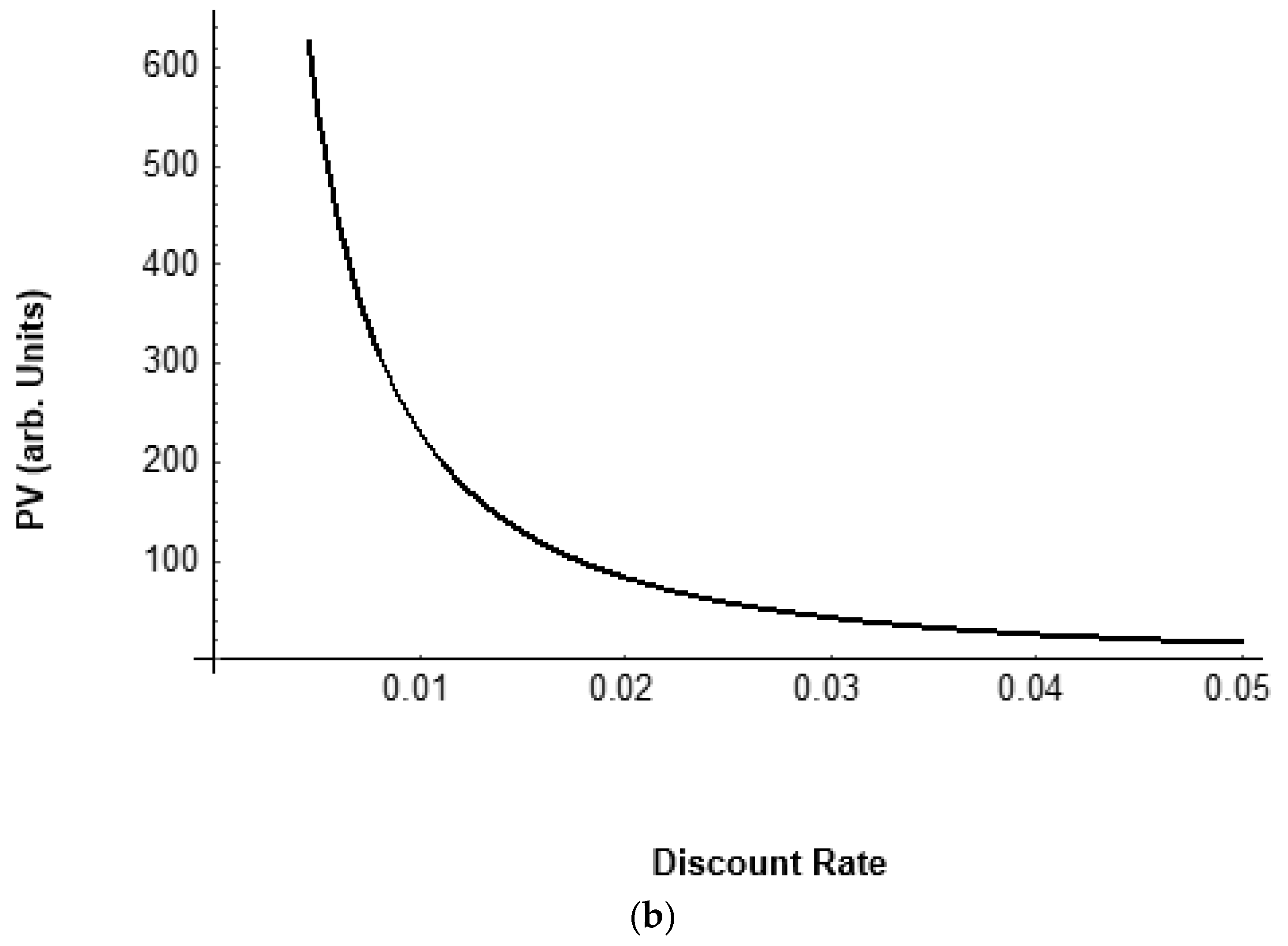
Figure 2.
(a) Harvest age based on the maximum PV for different discount rates using the Faustmann formula. At low discount rates, the rotation length approaches the age of the peak MAI (89 y in this case). (b) PV for various discount rates using the age of the max PV to determine the rotation length (stand scale). Calculations based on the Weibull function (Figure 1).


Figure 3.
Age distribution for ownerships of different sizes when stands are acquired by a landowner randomly over the ages of 1–40 years old (single realization of each case). Solid line = 100 stands. Dashed line = 1000 stands. Red line = 50,000 stands. The distribution converges to uniform with the number of stands, as expected.

Figure 4.
Harvest based on Figure 1 for a forest that is not regulated. The forest has an even age distribution between the ages of 1–100, but without stands between the ages of 40–59. The stands are harvested if they are at or above the rotation age. The initial harvest is large to capture all the stands above the rotation age. (a) Harvest each year for rotation age 89 showing very irregular harvests. (b) Average annual harvest for different rotation ages over a 20,000 yr simulation. The peak is at the age of the maximum MAI (age 89).


Figure 5.
Stumpage per ac for the combined pulpwood ($30/cord), chip-n-saw ($57/cord) and saw ($80/cord) in 1990 prices for loblolly in Georgia based on a growth model, site index 65 and planting density of 600 trees per acre from Yin (1997). For a risk of 1%, the yield curve bent downward (red).
Figure 5.
Stumpage per ac for the combined pulpwood ($30/cord), chip-n-saw ($57/cord) and saw ($80/cord) in 1990 prices for loblolly in Georgia based on a growth model, site index 65 and planting density of 600 trees per acre from Yin (1997). For a risk of 1%, the yield curve bent downward (red).

Figure 6.
MAI in dollars based on Figure 3. Since the income curve was virtually linear, the MAI curve had no peak. The penalty for a harvest at age 25 vs. age 40 was approx. 13%. For a 1% risk (red), the year of the peak MAI was age 29. Note that the curve was quite flat near the peak, meaning that a harvest flexibility existed.

Disclaimer/Publisher’s Note: The statements, opinions and data contained in all publications are solely those of the individual author(s) and contributor(s) and not of MDPI and/or the editor(s). MDPI and/or the editor(s) disclaim responsibility for any injury to people or property resulting from any ideas, methods, instructions or products referred to in the content. |
© 2023 by the author. Licensee MDPI, Basel, Switzerland. This article is an open access article distributed under the terms and conditions of the Creative Commons Attribution (CC BY) license (https://creativecommons.org/licenses/by/4.0/).
Share and Cite
MDPI and ACS Style
Loehle, C. Forest Land Expectation Value or Maximum Sustained Yield? Resolving A Long-Standing Paradox. Forests 2023, 14, 1052. https://doi.org/10.3390/f14051052
AMA Style
Loehle C. Forest Land Expectation Value or Maximum Sustained Yield? Resolving A Long-Standing Paradox. Forests. 2023; 14(5):1052. https://doi.org/10.3390/f14051052
Chicago/Turabian StyleLoehle, Craig. 2023. "Forest Land Expectation Value or Maximum Sustained Yield? Resolving A Long-Standing Paradox" Forests 14, no. 5: 1052. https://doi.org/10.3390/f14051052
Note that from the first issue of 2016, this journal uses article numbers instead of page numbers. See further details here.