Article

Assessment of Post-Fire Phenological Changes Using MODIS-Derived Vegetative Indices in the Semiarid Oak Forests

1
Department of Forest Science, Faculty of Agriculture, Ilam University, Ilam 516-69315, Iran
2
General Department of Natural Resources and Watershed Management of Ilam Province, Ilam 516-69315, Iran
3
Department of Plant, Food, and Environmental Sciences, Faculty of Agriculture, Dalhousie University, Truro, NS B2N 5E3, Canada
4
German Research Center for Artificial Intelligence, 26129 Oldenburg, Germany
5
John von Neumann Faculty of Informatics, Obuda University, 1034 Budapest, Hungary
*
Author to whom correspondence should be addressed.
Forests 2023, 14(3), 590; https://doi.org/10.3390/f14030590
Submission received: 11 January 2023 / Revised: 12 February 2023 / Accepted: 28 February 2023 / Published: 16 March 2023
(This article belongs to the Special Issue Soil and Plant Restoration after Wildfire)

Abstract

:
Wildfire has significant impact on plant phenology. The plants’ phenological variables, derived from time series satellite data, can be monitored and the changes in satellite imagery may be used to identify the beginning, peak, and end of the growing season. This study investigated the use of remote sensing data and land surface phenology (LSP) parameters to evaluate the impacts of fire. The LSP parameters included the start of growing season (SOS), the length of the growing season (LOS), the end of the growing season (EOS), maximum greenness of the season (Gmax), and minimum greenery in the season (Gmin) in the fire-impacted, semiarid oak forests of Iran. These LSP parameters were extracted from multitemporal normalized difference vegetation index (NDVI) and enhanced vegetation index (EVI2) data, acquired from MODIS sensor images in Zagros of the Ilam province in western Iran. By extracting LSP indices from the NDVI and EVI2 data, the indices were compared between burned forest areas, areas surrounding the burned forests, and unburned areas and for timesteps representing pre-fire, fire (i.e., year of fire), and post-fire (i.e., 2 years) conditions. It was found that for the burned area, there were significant differences in Gmax and the day that Gmax occurred. Furthermore, there was also a significant difference in Gmin between the pre- and post-fire conditions when NDVI was used and a significant difference between Gmax when EVI2 was used. The results also showed that in both time series there was a significant difference between the burned and control area in terms of Gmax. In general, the results showed that the fire had a negative effect on LSP, but in the two years after the fire, there were signs of forest restoration. This study provides necessary information to inform forest and resource conservation and restoration programs.

1. Introduction

Forest fires are one of the destructive factors and causes of forest degradation around the world [1,2,3]; hence, researchers and forest managers have identified the need to study the impacts of different fire intensities and histories in forested landscapes [4,5,6,7]. The forests of Zagros cover the northwestern to southeastern region of Iran and are considered as sub-Mediterranean forests. These forests provide a unique habitat for valuable species, such as the Persian oak (Quercus brantii L.), which is the dominant tree species, as well as habitats for other plant and animal species [8,9,10]. However, the increasing number of fires that were reported in the region over the past decade [11,12] have posed a serious threat to biodiversity and has changed the structure of these forests [13,14]. Although the ecological effects of fires on natural ecosystems have been widely studied, there is relatively little information about their impacts on the phenology of the ancient oak forests of western Iran. Plant phenology involves studying the lifecycle of plants (e.g., budbreak, leafing, flowering, fruiting, and leaf coloring), whereby the information about these lifecycle events and their timing provide useful indicators for monitoring climatic and environmental change [15,16] and understanding the relationships between seasonal changes and vegetative characteristics [17,18]. Furthermore, the phenological responses of plants to global climate change has been an increasingly important area of scientific research [19,20]. Although many ecologists have monitored and documented plant phenology in the field, scientific and technological advances have now made it possible to characterize plant phenology at wider spatial and temporal scales using cost-effective and time-efficient methods [21,22]. For example, advances in remote sensing have provided the necessary tools to study plant phenology—especially in environments with limited access, where direct measurements in the field are impractical [23,24]. Furthermore, multitemporal imagery, acquired by satellite sensors, provides the means to monitor vegetation dynamics throughout the ecosystem [25,26]. These advances have led to the emergence of a new scientific subdiscipline, land surface phenology (LSP) [27,28], which leverages a suite of vegetative indices to understand the seasonal patterns in plant phenophases. Over the past decades, LSP techniques have gained considerable attention due to their ability to analyze satellite-derived vegetative indices over time; provide information needed to determine the timing of vegetative growth [29]; and describe the interaction between vegetation and climate [30].
Phenological variables derived from time series satellite data can reflect changes in the start, end, or length of the vegetation growing season within a spatiotemporal context [31,32]. The timing and extent of the vegetation greenness provide insight into the vegetative response to changes in environment and management strategy [33]. Here, LSP techniques involve the calculation of vegetative indices, such as maximum seasonal greenness (Gmax) and minimum seasonal greenness (Gmin) to characterize vegetative growth processes [34]. It is also important to recognize that LSP-based indicators are strongly influenced by land disturbance, such as land degradation, land use change, and human activity [35,36]. In addition, another key factor that affects LSP includes wildfire, which can cause significant and sudden changes in forest composition and long-term forest dynamics [37,38]. Despite the usefulness and application of LSP techniques, their application has yet to be studied in the semi-arid forests of Iran.
Modern methods for monitoring fire behavior over wide large extents rely upon sensors mounted on terrestrial satellites. One of the remote sensing products commonly used to monitor fire activity is the MODIS sensor, which is a medium-resolution sensor that provides information at medium to high spatial resolutions for mapping and monitoring fire [39,40]. Among the many spectral indices that have been used, the most common include Normalized Difference Vegetation Index (NDVI) and Enhanced Vegetation Index (EVI2) [41,42]. Multiple studies have shown changes in LSP in various terrestrial ecosystems post-fire [32,37,43,44,45,46,47,48], wherein the changes are influenced by the severity and duration of the fire, as well as the type of vegetation in a region. Hence, by using remote sensing data, it is possible to apply LSP techniques to evaluate and understand the sensitivity of ecosystems to fire—especially given the increasing frequency of fires in recent decades and the current trend of climate change [49,50]. Given that the potential for fire is greater in arid and semi-arid regions, it is important to use post-fire monitoring tools to facilitate an understanding of the vegetation recovery process post-fire. This has led to the development of new approaches and technologies for extensive monitoring of these areas [51,52,53,54,55,56]. Due to the role of phenology in monitoring and predicting the timing of life cycle events of plants, phenology has gained particular importance in the current global change research. However, the use of phenological data in environmental protection and management is still poorly understood. Therefore, this study was conducted to investigate the phenological changes of the land surface after the fire using vegetation indices. The results can support the provision of protection and rehabilitation measures in fire-affected areas by increasing and improving the awareness of the existing conditions using remote sensing-based monitoring. Specifically, the objectives of this study were (1) to determine if fires cause delays in the phenological phases of the start of the growing season (SOS) and the end of growing season (EOS); (2) to evaluate the impact of fires on vegetative greenness in the semiarid ecosystems of Iran; and (3) to compare the suitability of NDVI and EVI2 in evaluating the impact of fires on LSP.

2. Materials and Methods
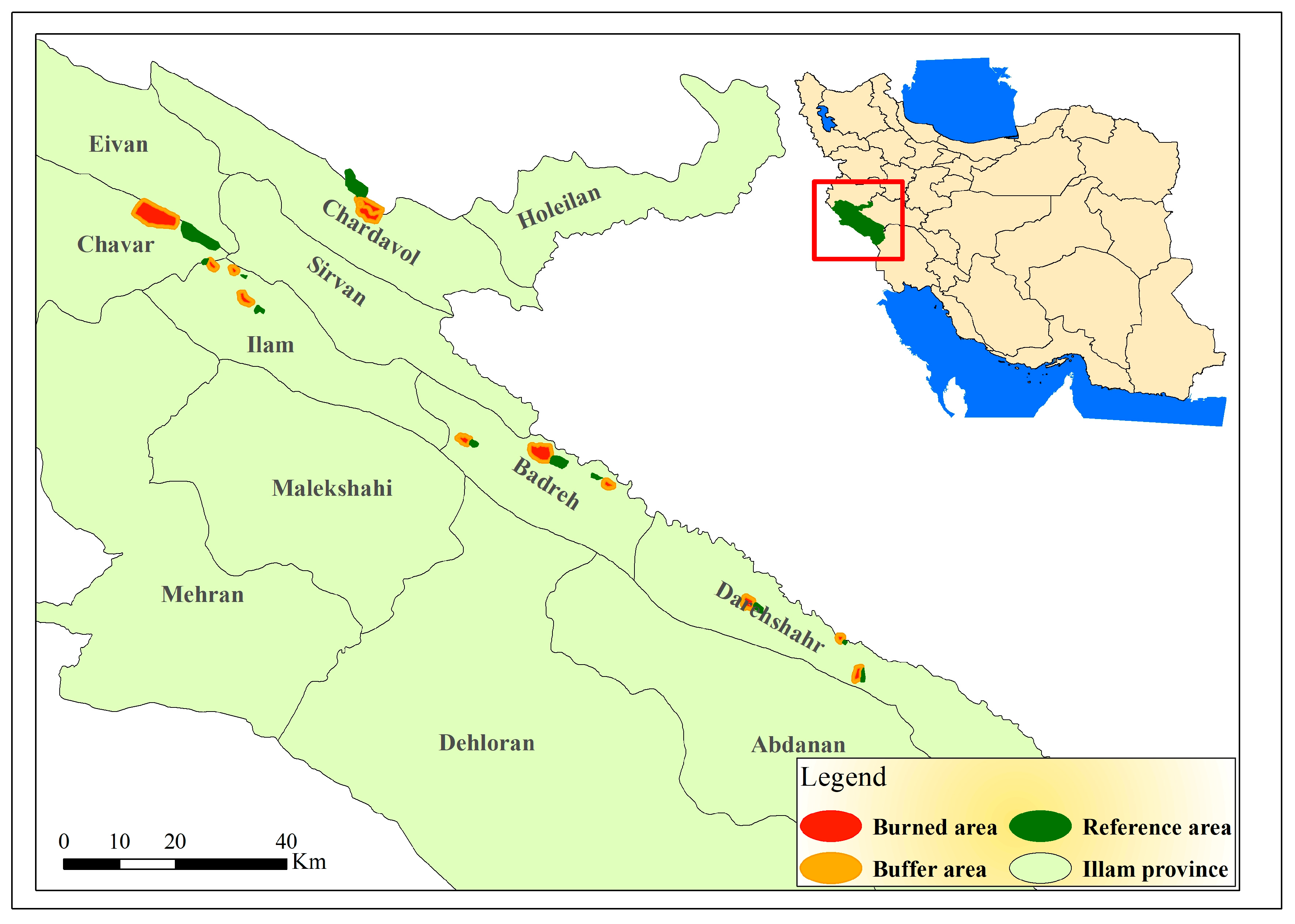
2.1. Study Area

This study was carried out in the natural landscapes of Ilam province in western Iran. As recorded by the Natural Resources Department of Ilam Province, this region has experienced fires between 2014 and 2020 (Figure 1). The study area is located 46°14′15″ E to 47°38′40″ E longitude and 33°49′33″ N to 32°58′12″ N latitude. Here, the elevation ranges from 472 to 1275 m above mean sea level. The climate is described as sub-Mediterranean and semi-arid temperate and has dry summers and mild-to-cold winters. Based on meteorological information, the average temperature varies from 16.9 °C in the north to 21.5 °C in the southwest and the average annual rainfall is 500.3 mm per year. The vegetation is dominated by Persian oak (Quercus brantii Lindl.) and various other subdominant wood species, such as Crataegus pontica C. Koch, Pistacia atlantica Desf., Acer monspessulanum L., and Daphne mucronata Royle. The forest undergrowth is comprised of various annual and perennial species. The combination of climatic conditions and vegetation puts this region at risk of fires each year.

2.2. Identification of Fire Impacted Areas

To investigate the impact of fires on land cover phenology, fires were first identified from natural habitats (e.g., forests and pastures). Here, 13 large fires that occurred in the province between 2014 and 2020, and with an area of >45 ha, were selected. Information on the fires was registered and mapped by the Department of Natural Resources of Ilam Province. To evaluate the effects of the fire on the boundaries of the burned areas, which were less impacted by fires, a buffered region of 500 m from these burned areas was investigated. This was used as the ‘buffer zone’ treatment for our comparisons with the fire-impacted treatment. Furthermore, reference areas (i.e., control) were established at >500 m from each burned area. The reference areas were selected with the purpose of controlling the impacts of changing environmental (e.g., vegetation and topography) and climatic conditions (Figure 1).

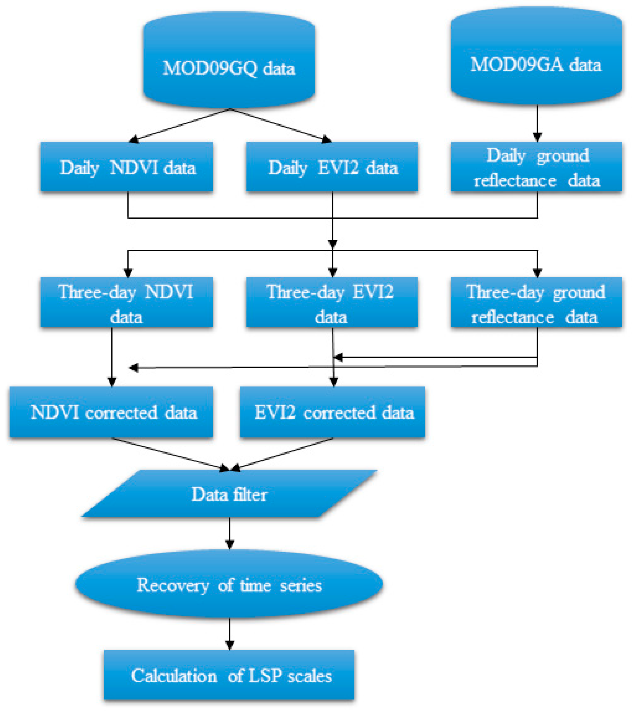
2.3. Acquisition of Remote Sensing Data

To analyze the effects of fire on forest phenology from 2014 to 2020, time-series MODIS imagery was acquired for the burned, buffered, and control areas and used to evaluate the daily ground cover. Here, the MOD09GA and MOD09GQ MODIS products were acquired. Both MODIS products have a daily temporal resolution; however, the MOD09GQ data were distributed at a 250 m spatial resolution while the MOD09GA data were at a 1 km spatial resolution. The MOD09GA data were resampled to a 250 m spatial resolution using a nearest-neighbor approach to ensure comparability with the MOD09GQ product. Both the MOD09GQ and MOD09GA data had two bands: Band 1 (red; 620–670 nm) and Band 2 (near infrared; 841–876 nm)—both of which were radiometrically and atmospherically corrected. Using these two bands, NDVI [57] and EVI2 [58] were calculated as follows:
NDVI = (NIR − Red)/(NIR + Red)
EVI2 = 2.5 × s (NIR − Red)/(NIR + 2.4Red + 1)
where NIR and Red represent the reflectance values for the near-infrared and red bands. The NDVI varies between −1 and +1, wherein large positive values indicate high vegetative greenness, while smaller positive values indicate lower vegetative green [59,60]. Values close to 0 often correspond to bare rock or earth, while negative values are usually caused by clouds, snow, ice, or water [61]. One limitation of NDVI is that different environmental processes may result in the same value; for example, if fire causes the transition of pastures to shrublands, the NDVI may remain constant because the amount of productive biomass remains constant [62,63]. To address the limitation of NDVI, EVI2 was also included in this study due to its improved sensitivity for areas with high biomass; furthermore, its decreased sensitivity to atmospheric influences and the background signal of the canopy improves its ability to support the monitoring of vegetation [64,65]. In many studies, NDVI and EVI2 have been useful for LSP characterization. Given the large number of images that were required to be processed, the daily temporal resolution was reduced to a 3-day resolution where the best imagery for every three days was retained. The data reduction process assumed that changes in forest surface phenology over the course of three days were negligible and would not affect the accuracy of LSP parameters [66]. As a result, the NDVI and EVI2 were calculated for 540 images acquired between February to October and from 2014 to 2020. To filter the data and reduce the noise in the calculation of phenological criteria, a Savitzky–Golay filter was applied. This filter was described by Jonsson and Eklundh [67].

2.4. Land Surface Phenology Parameters

The NDVI and EVI2 were used to calculate LSP indices, which corresponded to the start of the growing season (SOS), end of the growing season (EOS), length of the growing season (LOS), maximum greenness of the season (Gmax), and minimum greenness of the season (Gmin) during the time before a fire and two years post-fire for the burned, buffer, and control areas. As presented in Figure 2, adapted from [17], these LSP metrics were calculated based on the NDVI and EVI2 time series and based on the maximum or minimum change in the pixel magnitude curve [68].
To prepare a phenological map and investigate the LSP changes due to the fire while accounting for the effects of climatic and environmental factors, each LSP parameter was calculated for the before and after the fire periods using the following equations [34]:
LSP anomaly = LSP after fire in reference − LSP before fire in reference
LSP change = (LSP after fire − LSP before fire) − LSP anomaly
Here, the LSP anomaly shows the effect of climatic factors on LSP changes and the degree of LSP changes before and after the fire in the control area. Figure 3 shows the methodological framework of this study. Here, the daily data were first converted to three-day data to reduce the volume of data; the vegetation indices were produced; lastly, LSP indices, using the time series data and filter, were calculated.

2.5. Statistical Design

The temporal effects of the fire (i.e., before the fire, directly after the fire, and 2 years after the fire) on each of the LSP parameters were determined using individual one-way analysis of variance (ANOVA) for the burned, buffered, and control areas. A Duncan’s new multiple range test was carried out to provide statistical comparisons of the mean values of each LSP parameter between the treatments. Furthermore, an independent Student’s t-test was used to compare between NDVI and EVI2 values.

3. Results

After preparing the NDVI and EVI2 indices from the MODIS imagery, and extracting the phenological characteristics (i.e., Gmax, Gmin, SOS, EOS and LOS) using NDVI and EVI2, the values of each LSP parameter were compared between the pre-fire, directly after fire, and 2-years post fire timesteps and between the fire, buffered (i.e., region within a 500 m distance from the fire), and control regions (i.e., region beyond a 500 m distance from the fire).

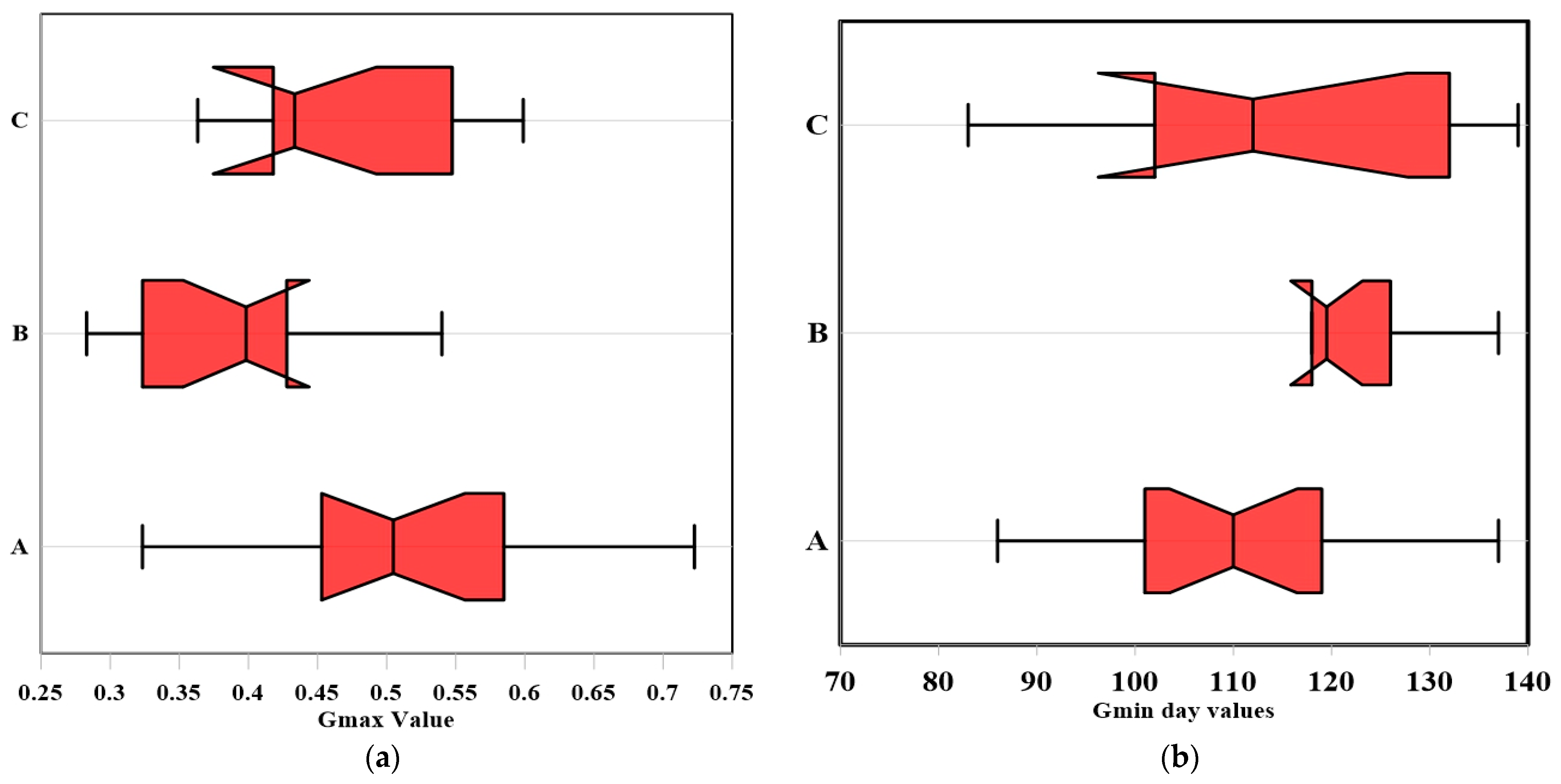
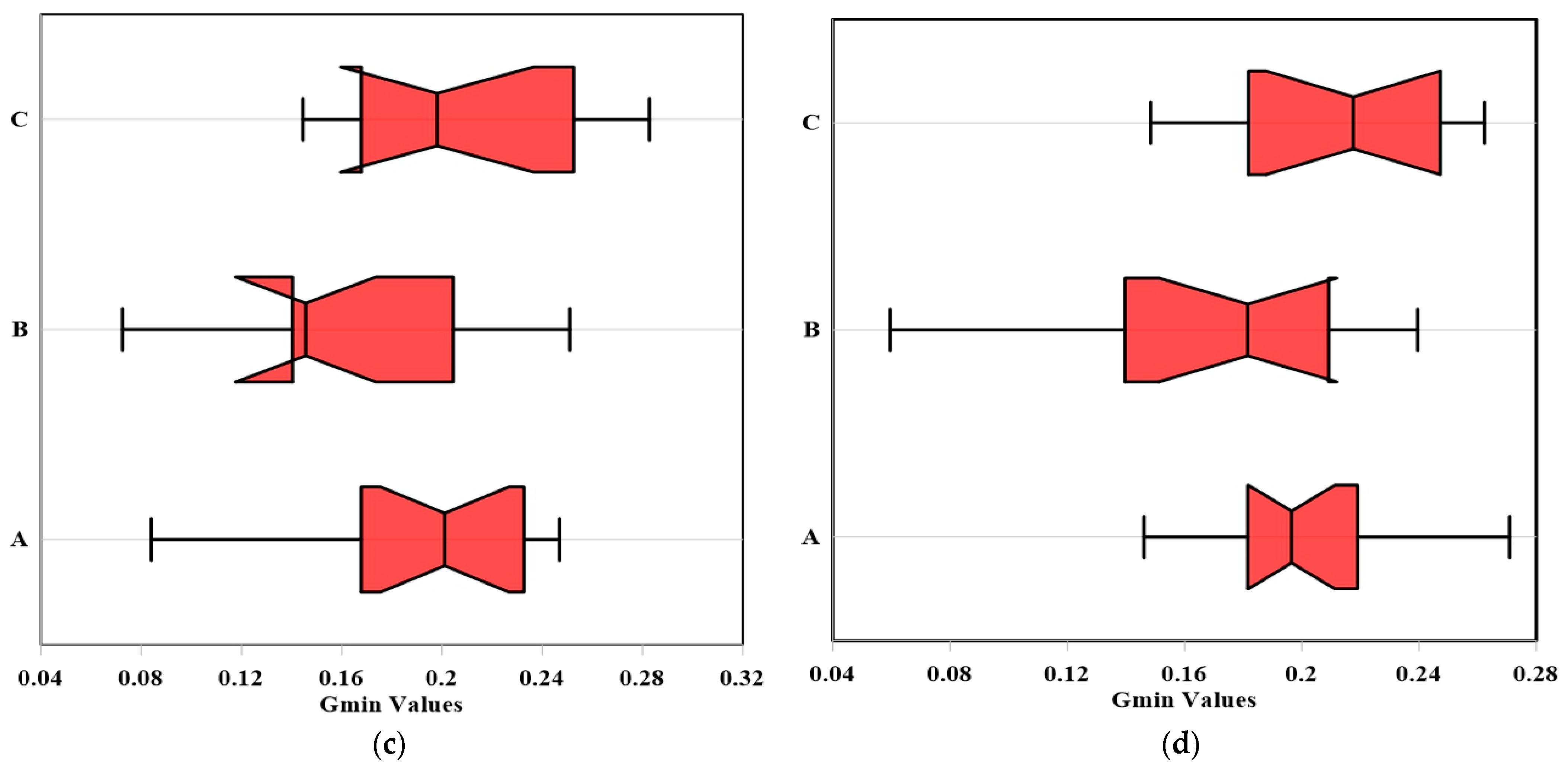
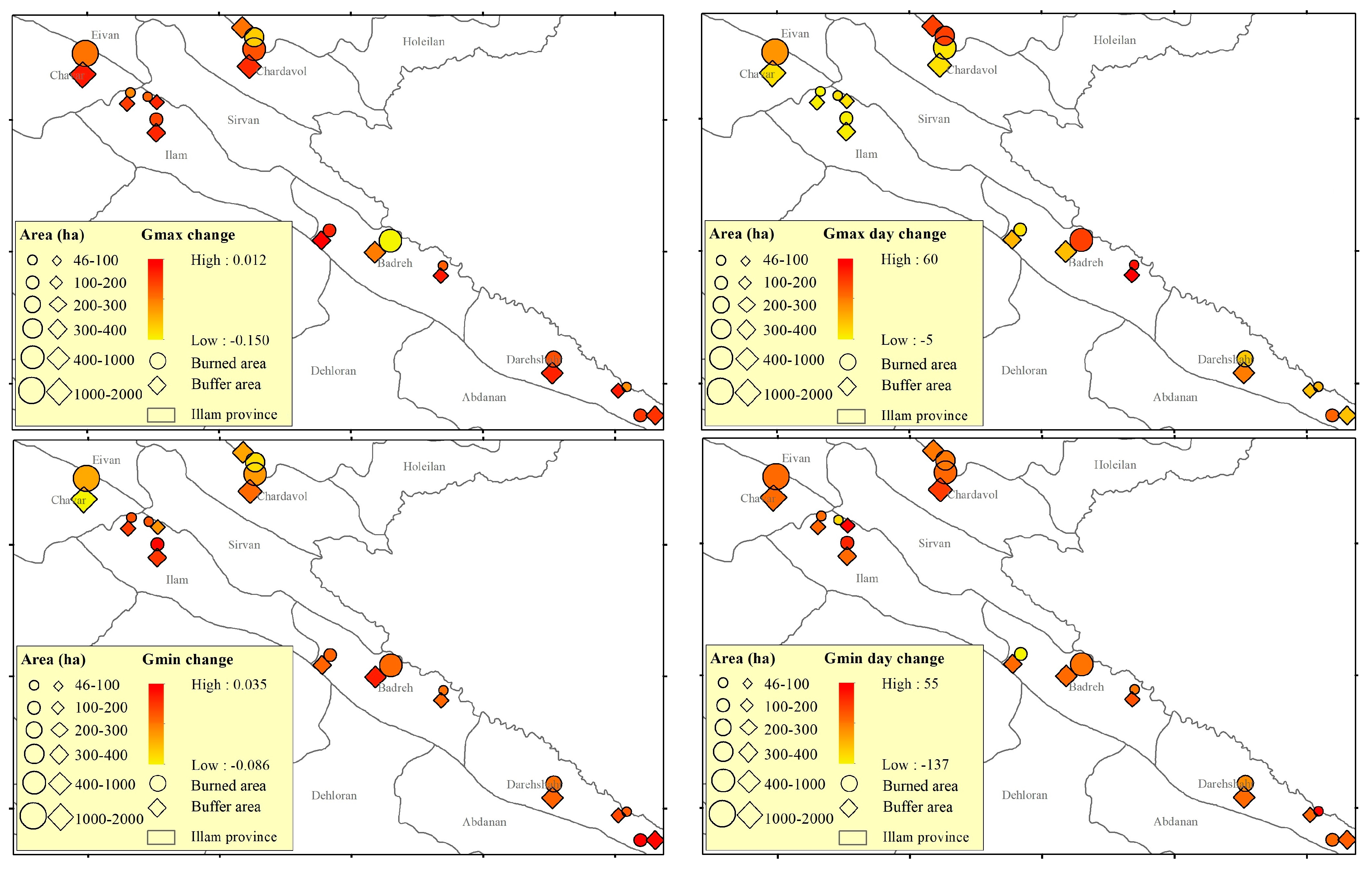
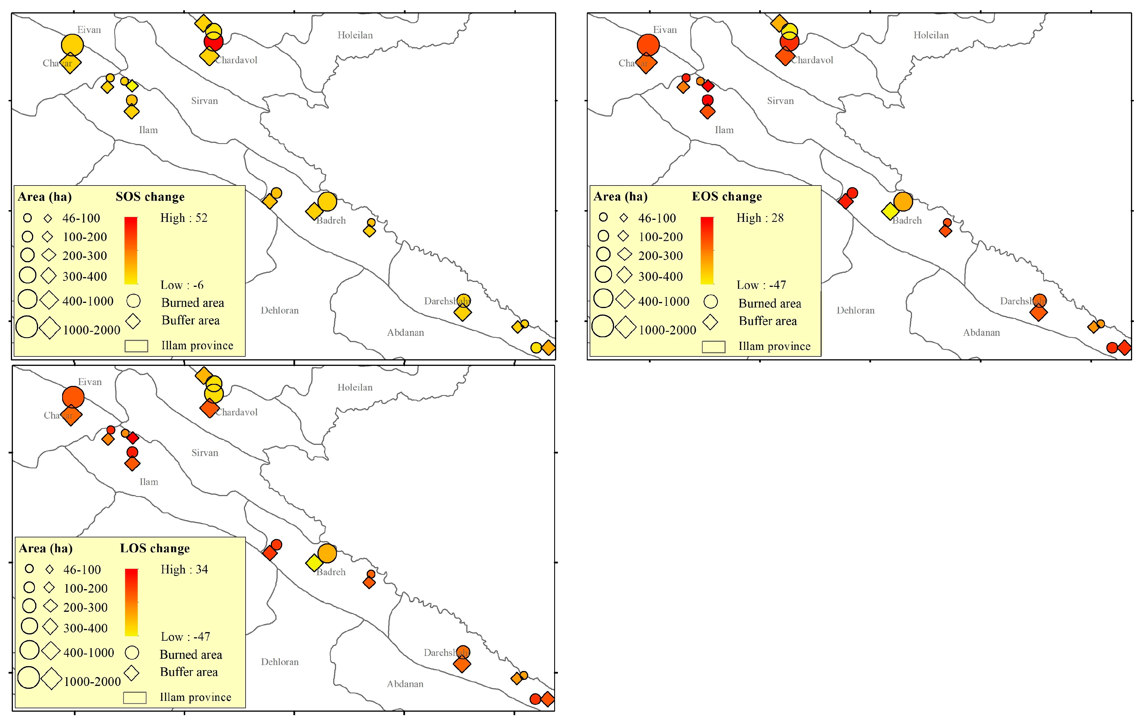
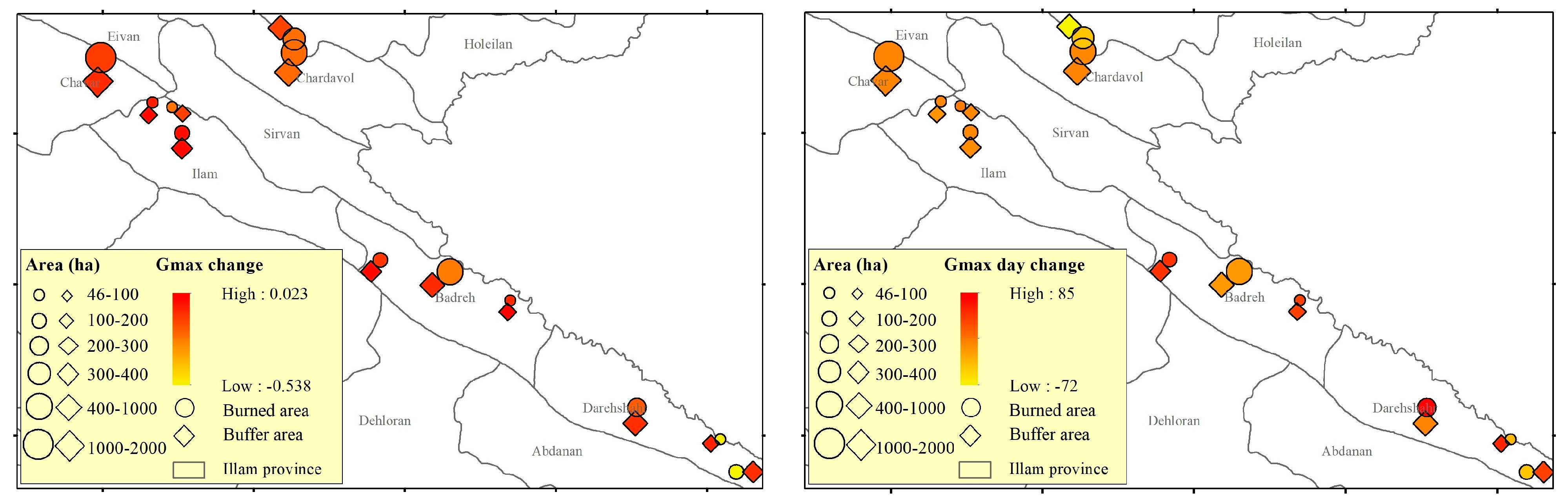
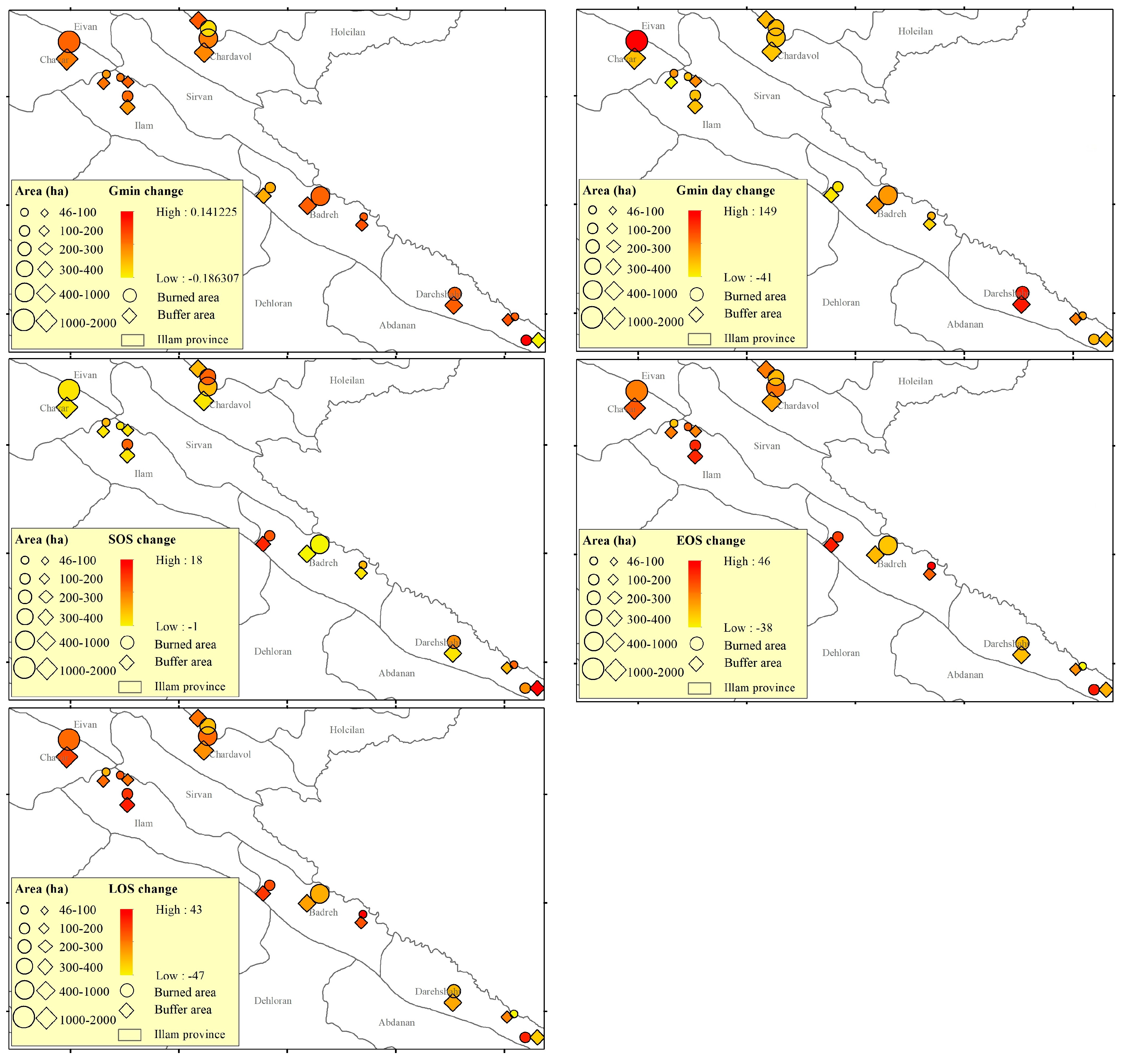
3.1. Impacts of Fire on Land Surface Phenology

3.1.1. Normalized Difference Vegetation Index (NDVI)

The results from the analysis of variance showed that in the burned area, there was a significant difference between, Gmax, the Gmax Day, and Gmin between the before and after fire periods. With respect to the other characteristics, such as the Gmin Day, SOS, EOS and LOS, there were no significant difference observed. There was a significant difference in terms of Gmax between the pre-fire period, immediate after the fire, and the two-year period after the fire. However, there was no significant difference with the pre-fire period, indicating that the forests were experiencing recovery from the fire. For Gmax Day and Gmin, there was a significant difference (p < 0.05) between the pre-fire and the second year after the fire. For the buffered zone, the results also showed that there was a significant difference before and after the fire for only Gmin; however, no significant differences were observed in relation to the other properties. There was also a significant difference between the time of the fire and two years after the fire (Table 1). For the control area, as expected, no significant difference was observed between before and after the fire.
Figure 4 and Figure 5 further illustrate the difference between the LSP criteria using NDVI for periods before and after the fire. Due to the fire, the Gmax for all burned areas and for >90% of buffered areas decreased; furthermore, the Gmin for >83% of the burned areas and >66% of fire buffered areas also decreased. Both Gmax and Gmin were reduced due to fire—in >83% of the burned and buffered areas, the fire delayed the occurrence of Gmax. In the case of Gmin day, the opposite was true, with 50% of Gmin burnt areas occurring on the day before the Gmin day and before the fire, which meant that the fires resulted in an earlier Gmin day. In most cases, the fire delayed the Gmin day.
The start of the growing season remained unchanged for 40% of the burned areas and delayed the onset of the growing season from 3 to 50 days for 45% of the burned areas but did not change the start of the growing season for 75% of the buffered areas. However, for 60% of the fires that occurred, the fire resulted in an earlier end to the growing season and thus reduced it as well. Overall, in burnt areas, the fires delayed the start of the growing season by 4.58 days and accelerated the end of the growing season by 0.6 days, resulting in a reduction of the growing season by an average of 2.5 days. In the buffered areas, the length of the growing season was reduced by 3 days because of fire.

3.1.2. Enhanced Vegetation Index (EVI2)

When using EVI2, only Gmax resulted in a significant difference when comparing between the pre-fire and year of the fire; however, after two years, the EVI2 returned to pre-fire levels. When compared with using NDVI for evaluating LSP changes, EVI2 was less sensitive (Table 2). Figure 6 shows the boxplots of Gmax for each time step. Based on the results, there was a significant difference between the year of the fire with the year before the fire and two years after the fire. Figure 7 also shows the map of changes in LSP characteristics due to fire. Similar to the NDVI results, the EVI2 metric produced Gmax values that were 93% lower and Gmin values that were 83% higher for the burned areas in comparison with the buffer areas. In reviewing the results using EVI2, it was found that at the beginning of the growing season in burned areas, >80% of burned areas were delayed by 3 to 10 days and had an average delay of 5 days. When compared with the end of the growing season, which had an average delay of 3 days, there was a reduction in the length of the growing season by about 2 days due to fire—similar to the findings when NDVI was used. The reduction of the growing season due to fire in buffer areas was approximately equal to a decrease of 0.1 days.

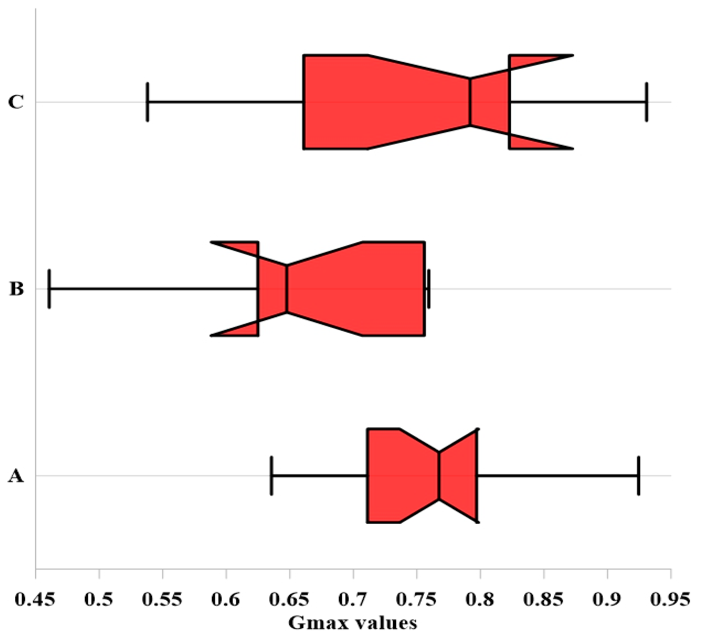
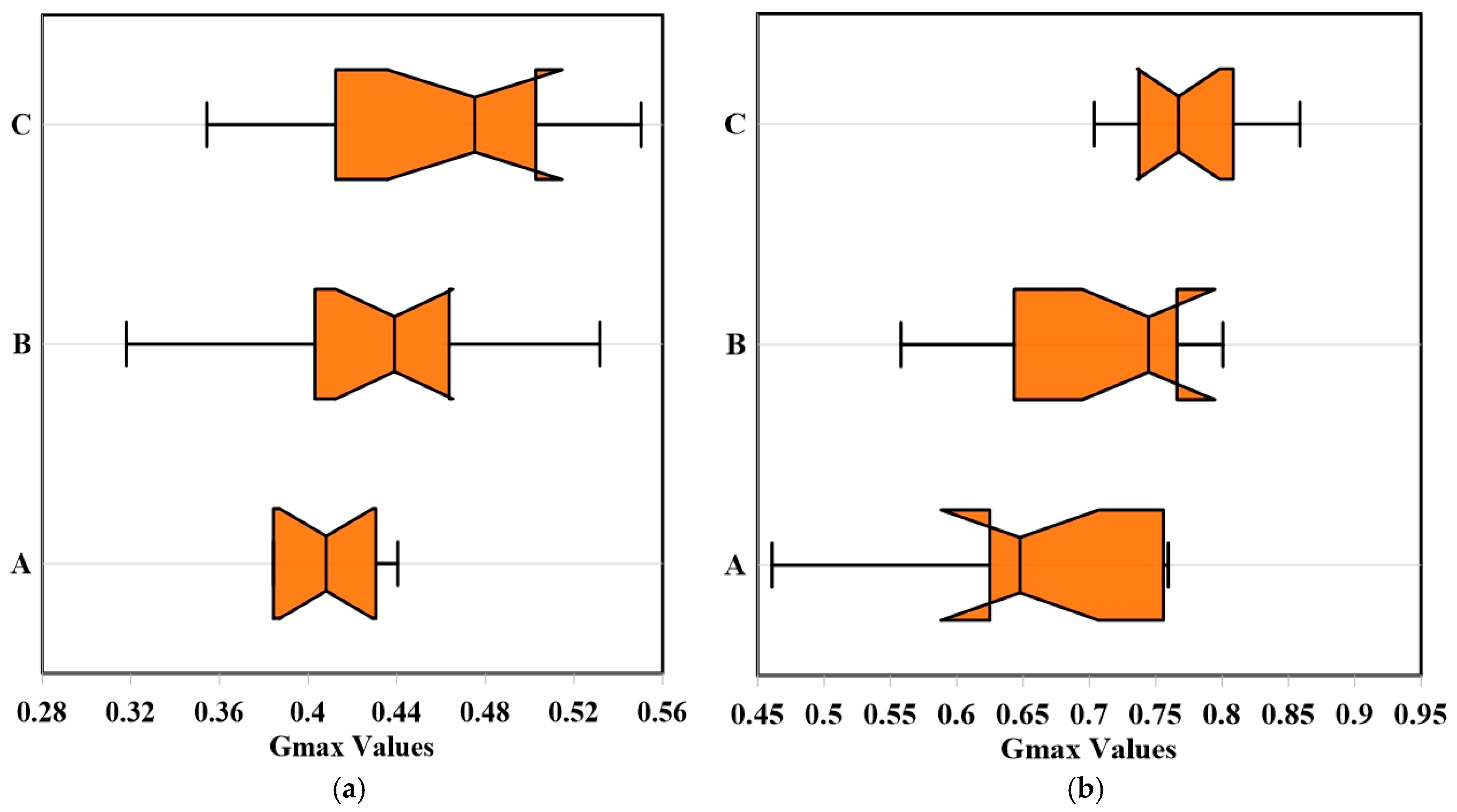
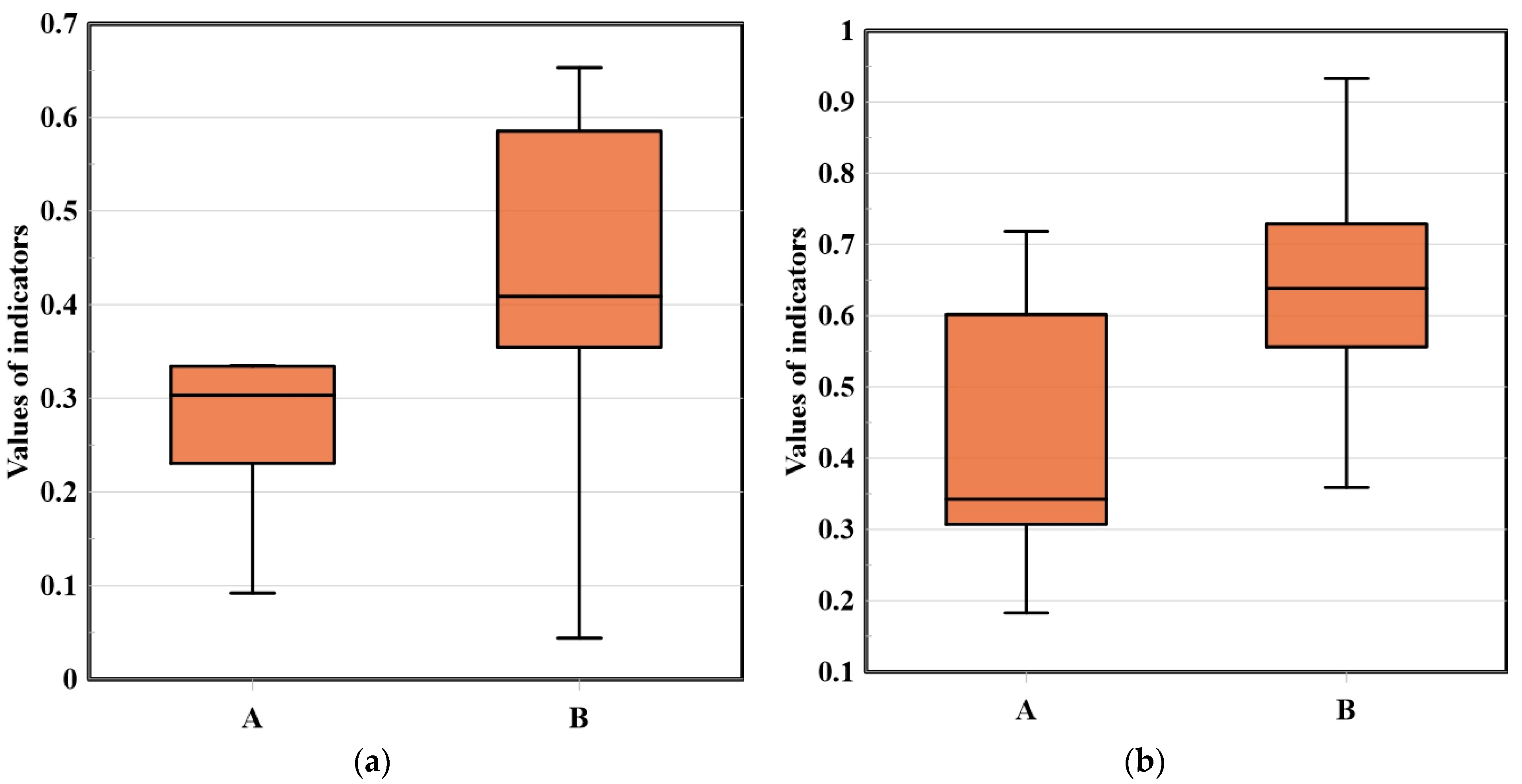
3.2. Comparison of Land Surface Phenology

The results of comparing LSP indices between the burned, buffered, and control areas after the fire showed that for both indices, despite the difference between the areas, only Gmax had significant differences. Based on the results, there was a significant difference between the burned and control areas based on NDVI and EVI2; however, there was no significant difference between the burned and buffer areas, as well as the buffer and control (Table 3). The Gmax boxplot between the burned, buffered, and control areas is also shown in Figure 8.

3.3. Comparison of NDVI and EVI2

This study showed the potential for differences in LSP when NDVI and EVI2 were compared using an independent t-test was used. The results showed that the only LSP indicator that consistently resulted in a significant difference between the year of fire and two years after the fire, for both NDVI and EVI2, was Gmax. Here, the Gmax values from the NDVI and EVI2 indices had p-values of 0.014 and 0.008, respectively. The boxplots of these two indices are shown in Figure 9, which show that the values obtained from the EVI2 were higher than those of the NDVI.

4. Discussion

4.1. Influence of Fires on NDVI and EVI2

The results showed significant differences in LSP parameters when calculated using NDVI and EVI2—especially with Gmax—for the pre- and post-fire conditions. The results also showed a higher sensitivity of NDVI for detecting the difference in LSP parameters in comparison with EVI2. Many studies have emphasized the usefulness of NDVI in comparison with other indices [69,70,71,72,73]; for example, Falahatkar et al. [74] found that the NDVI was more correlated with broadleaf species because they have wider leaves and the way their leaves grow causes greater reflection from the leaf surface. As a result, this may possibly explain the effectiveness of NDVI for determining LSP parameters—especially given the prevalence of broadleaf species throughout the study.

4.2. Influence of Fires on Vegetative Greenness

By comparing the greenness criteria between the pre- and post-fire conditions, it was observed that there was a significant difference between Gmax, Gmin, and Gmax (day) in the burned areas where Gmax and Gmin were reduced in the burned areas. To a lesser extent, a decrease was also observed in the buffer zone; however, the magnitude of the change was lower when compared with the burned areas. A delay in Gmax was seen in >83% of the burned areas and a delay in Gmax for 50% of the burned areas. As expected, the Gmin was higher in the early years; however, Gmax was the opposite, whereby two years post-fire, there were signs of vegetation restoration. Comparing the greenness between the areas, a significant decrease was observed between the burned and control areas, which was also expected due to the destructive behavior or the fire. Although studies, such as Zhang et al. [34], have also shown a decrease in greenness due to fires, few studies examined the impact of fires on phenology, as most studies were related to the temporal dynamics of plant growth (e.g., SOS, EOS, and LOS).
One potential factor for the reduced vegetative greenness could be due to the presence of therophyte and invasive species as they are able to establish their own structural system, multiply rapidly, and dominate the environment. However, these species have a limited lifespan and vegetative cover; therefore, the tree species are still able to regenerate the fire-impacted landscape and have the potential to regenerate the forest into a pre-fire state. Other studies have also reported the predominance of therophytes during fires [75,76]. It should also be noted that satellite imagery was used to classify land cover for the entirety of pixels; hence, if the imagery lacks a sufficiently fine spatial resolution, it would not be able to detect sub-pixel changes in vegetation—especially therophyte and invasive species in the burned areas, which often have low volumetric coverage, as well as high-pitched canopies. The lower-canopy is also less detectable by satellites, which may decrease the greenness [76].

4.3. Impact of Fire on Growth Time

The results showed a delay in SOS, which was followed by an earlier EOS, thus reducing the vegetation growing season. The results of our study showed immediate, negative effects on vegetative phenophases—although these effects were not significant. Although our findings were consistent with numerous other studies, e.g., [77,78,79,80,81,82,83,84,85], other studies found contradictory results, e.g., [86,87,88]. The reason for these differences may have been related to the dependence of the phenological cycle on environmental factors and stressors, such as drought, fire, soil erosion, and soil properties, as well as climatic and anthropogenic (e.g., land use and land cover change). Although the climatic impacts on phenological processes are undeniable, e.g., [89,90,91,92], in some cases, forest disturbances may override the climatic factors [76]—especially in forests. As a result, the impact of fire, in some cases, depends on the environmental conditions prior to the fire wherein more productive forests, prior to a fire, are likely to remain productive after a fire. However, this was not the case here as the forests had an initially thin cover. According to Staver et al. [93], in forests with a canopy cover of <40%, the fire may impact plant growth pathways where the heat from fire may disrupt reproductive structures and processes, such as flowering, germination, and fruiting [94]. Furthermore, the fires may damage roots and rhizomes needed for post-fire reproduction [95] or even destroy the seed bank of the species. Some fires also cause soil degradation via loss of soil nutrients, structure, and microorganisms [96,97,98].
Post-fire, some species are unable to adapt to the new environmental conditions and are eliminated [75]. Thus, only species that are resilient to fire remain, such as the oak species (a dominant species in the Mediterranean), which is effective in regeneration well after a fire. Barton and Poulos [99] reported that in Arizona, USA, pine forests that were impacted by fire were converted into forest stands that were dominated by oak and oak shrubs. This study demonstrated the regenerative capacity of the oak species. It should also be noted, however, that the methods used for this study did not allow for the identification of individual species and that the LSP parameters may also have been influenced by the presence of other woody or herbaceous plants. This study also showed that fires resulted in an overall acceleration of the EOS and where the change in EOS was greater than that of the changes in SOS. Fire may shorten the end of the growing season. This may be related to the change in diversity of plant species [34] and their distribution following the fire in different ecosystems, such as temperate deciduous forests [100] and broad-leaved mixed forests [101]. However, it is also important to recognize the uncertainties in estimating and evaluating EOS due to the complex interactions between climatic, environmental, and human factors compared with other phenophases [102]. It is possible that the earlier EOS could be attributed to the reduction of tree cover, which would lead to a decrease in canopy level and the delay in canopy development due to the fire. Furthermore, the aging of trees may also be affected; for example, Fuller et al. [103] found that areas with relatively low canopy closure aged earlier than for dense canopy forests; Miombo. Cho et al. [104] showed that phenological changes at the end of the growing season were usually determined by a fraction of tree cover in the South African savannah forests.
As the canopy coverage decreases, the soil temperature naturally increases and has a direct effect on soil temperature. In deciduous forests, the temperature may be negatively correlated with the history of EOS because temperature increases the root respiration by trees and without sufficient soil moisture, there is less water uptake, thereby causing an earlier EOS. Despite the importance of temperature as a control of EOS [105], it should be noted that the leaves of deciduous trees need a certain accumulated temperature for growth and the increase in pre-season temperature causes the leaves of the trees to reach the required accumulated temperature in a shorter time, resulting in earlier wilting dates EOS [105,106]. For this study area, which is mostly dominated by herbaceous and invasive plants because of fire, the warmer temperatures during the season accelerated the end of the growing season, which is consistent with Fu et al. [105]. Furthermore, the acceleration of EOS affected subsequent events [107] and hence, there was a negative relationship between SOS and EOS. It was also possible that, due to the fire, there was a corresponding decrease in soil moisture, which limited vegetation growth and suppressed ecosystem productivity [107].

5. Conclusions

This study examined how multitemporal remote sensing data could be used to evaluate the impact of fire on LSP in a semiarid forest ecosystem. Amongst the LSP parameters, the Gmax for both vegetation indices (NDVI and EVI2) was significantly different between the year of the fire and two years after the fire. It was also observed that the fire had a negative impact on SOS and EOS by delaying SOS and accelerating EOS; however, the impacts of the fire were more evident on the vegetative greenness. These results were expected given the semiarid conditions of the region. The results also showed that NDVI was more sensitive in detecting the differences in LSP in comparison with EVI2. Although the study highlighted the destructive impacts of fire, there were also signs of vegetation restoration two year after the fire. This may be related to the presence of oak as a dominant species, which has a high potential for resprouting. Although this may seem promising, the fires change the form of oak forests from a mature state to a coppice state; as a result, the techniques used in this study provide the means to guide monitoring of forest resources and inform management strategies that facilitate forest regeneration.

Author Contributions

Conceptualization, S.K., M.H., J.M., O.K., B.H. and A.M.; methodology, S.K., M.H., J.M., O.K., B.H. and A.M.; software, S.K., M.H., J.M., O.K., B.H. and A.M.; validation, J.M., O.K., B.H. and A.M.; formal analysis, S.K., M.H., J.M., O.K., B.H. and A.M.; investigation, S.K., M.H., J.M., O.K., B.H. and A.M.; resources, S.K., M.H., J.M., O.K., B.H. and A.M.; data curation, S.K. and M.H.; writing—original draft preparation, S.K., M.H., J.M., O.K., B.H. and A.M.; writing—review and editing, S.K., M.H., J.M., O.K., B.H. and A.M.; visualization, S.K., M.H. and J.M.; supervision, M.H., B.H. and A.M.; project administration, M.H. and A.M.; funding acquisition, S.K., M.H., J.M., O.K., B.H. and A.M.; All authors have read and agreed to the published version of the manuscript.

Funding

This research received no external funding.

Data Availability Statement

Data is available upon reasonable request for the academic purposes through the corresponding or last author.

Conflicts of Interest

The authors declare no conflict of interest.

References

  1. Meng, R.; Wu, J.; Zhao, F.; Cook, B.D.; Hanavan, R.P.; Serbin, S.P. Measuring short-term post-fire forest recovery across a burn severity gradient in a mixed pine-oak forest using multi-sensor remote sensing techniques. Remote Sens. Environ. 2018, 210, 282–296. [Google Scholar] [CrossRef]
  2. Ling, L.; Fu, Y.; Jeewani, P.H.; Tang, C.; Pan, S.; Reid, B.J.; Xu, J. Organic matter chemistry and bacterial community structure regulate decomposition processes in post-fire forest soils. Soil Biol. Biochem. 2021, 160, 108311. [Google Scholar] [CrossRef]
  3. Lucas-Borja, M.E.; Delgado-Baquerizo, M.; Muñoz-Rojas, M.; Plaza-Álvarez, P.A.; Gómez-Sanchez, M.E.; González-Romero, J.; de las Heras, J. Changes in ecosystem properties after post-fire management strategies in wildfire-affected Mediterranean forests. J. Appl. Ecol. 2021, 58, 836–846. [Google Scholar] [CrossRef]
  4. Marlon, J.R.; Bartlein, P.J.; Gavin, D.G.; Long, C.J.; Anderson, R.S.; Briles, C.E.; Brown, K.J.; Colombaroli, D.; Hallett, D.J.; Power, M.J.; et al. Long-term perspective on wildfires in the western USA. Proc. Natl. Acad. Sci. USA 2012, 109, E535–E543. [Google Scholar] [CrossRef] [Green Version]
  5. Pechony, O.; Shindell, D.T. Driving forces of global wildfires over the past millennium and the forthcoming century. Proc. Natl. Acad. Sci. USA 2010, 107, 19167–19170. [Google Scholar] [CrossRef] [Green Version]
  6. Heydari, M.; Moradizadeh, H.; Omidipour, R.; Mezbani, A.; Pothier, D. Spatio-temporal changes in the understory heterogeneity, diversity, and composition after fires of different severities in a semiarid oak (Quercus brantii Lindl.) forest. Land Degrad. Dev. 2020, 31, 1039–1049. [Google Scholar] [CrossRef]
  7. Rostami, A.; Shah-Hosseini, R.; Asgari, S.; Zarei, A.; Aghdami-Nia, M.; Homayouni, S. Active Fire Detection from Landsat-8 Imagery Using Deep Multiple Kernel Learning. Remote Sens. 2022, 14, 992. [Google Scholar] [CrossRef]
  8. Salehi, A.; Heydari, M.; Poorbabaei, H.; Rostami, T.; Begim Faghir, M.; Ostad Hashmei, R. Plant species in Oak (Quercus brantii Lindl.) understory and their relationship with physical and chemical properties of soil in different altitude classes in the Arghvan valley protected area, Iran. Casp. J. Environ. Sci. 2013, 11, 97–110. [Google Scholar]
  9. Kazemi, S.M.; Hosseinzadeh, M.S. High diversity and endemism of herpetofauna in the Zagros mountains. Ecopersia 2020, 8, 221–229. [Google Scholar]
  10. Hosseini, S.P.; Jafari, R.; Esfahani, M.T.; Senn, J.; Hemami, M.R.; Amiri, M. Investigating habitat degradation of Ursus arctos using species distribution modelling and remote sensing in Zagros Mountains of Iran. Arab. J. Geosci. 2021, 14, 2179. [Google Scholar] [CrossRef]
  11. Moradizadeh, H.; Heydari, M.; Omidipour, R.; Mezbani, A.; Prévosto, B. Ecological effects of fire severity and time since fire on the diversity partitioning, composition and niche apportionment models of post-fire understory vegetation in semi-arid oak forests of Western Iran. Ecol. Eng. 2020, 143, 105694. [Google Scholar] [CrossRef]
  12. Bashari, H.; Naghipour, A.A.; Khajeddin, S.J.; Sangoony, H.; Tahmasebi, P. Risk of fire occurrence in arid and semi-arid ecosystems of Iran: An investigation using Bayesian belief networks. Environ. Monit. Assess. 2016, 188, 531. [Google Scholar] [CrossRef]
  13. Pourreza, M.; Hosseini, S.M.; Sinegani, A.A.S.; Matinizadeh, M.; Dick, W.A. Soil microbial activity in response to fire severity in Zagros oak (Quercus brantii Lindl.) forests, Iran, after one year. Geoderma 2014, 213, 95–102. [Google Scholar] [CrossRef]
  14. Heydari, M.; Rostamy, A.; Najafi, F.; Dey, D.C. Effect of fire severity on physical and biochemical soil properties in Zagros oak (Quercus brantii Lindl.) forests in Iran. J. For. Res. 2017, 28, 95–104. [Google Scholar] [CrossRef]
  15. Uphus, L.; Lüpke, M.; Yuan, Y.; Benjamin, C.; Englmeier, J.; Fricke, U.; Menzel, A. Climate Effects on Vertical Forest Phenology of Fagus sylvatica L., Sensed by Sentinel-2, Time Lapse Camera, and Visual Ground Observations. Remote Sens. 2021, 13, 3982. [Google Scholar] [CrossRef]
  16. Gray, R.E.; Ewers, R.M. Monitoring forest phenology in a changing world. Forests 2021, 12, 297. [Google Scholar] [CrossRef]
  17. Melaas, E.K.; Sulla-Menashe, D.; Gray, J.M.; Black, T.A.; Morin, T.H.; Richardson, A.D.; Friedl, M.A. Multisite analysis of land surface phenology in North American temperate and boreal deciduous forests from Landsat. Remote Sens. Environ. 2016, 186, 452–464. [Google Scholar] [CrossRef]
  18. Richardson, A.D.; Keenan, T.F.; Migliavacca, M.; Ryu, Y.; Sonnentag, O.; Toomey, M. Climate change, phenology, and phenological control of vegetation feedbacks to the climate system. Agric. For. Meteorol. 2013, 169, 156–173. [Google Scholar] [CrossRef]
  19. Tong, X.; Tian, F.; Brandt, M.; Liu, Y.; Zhang, W.; Fensholt, R. Trends of land surface phenology derived from passive microwave and optical remote sensing systems and associated drivers across the dry tropics 1992–2012. Remote Sens. Environ. 2019, 232, 111307. [Google Scholar] [CrossRef]
  20. Dannenberg, M.P.; Song, C.; Hwang, T.; Wise, E.K. Empirical evidence of El Niño—Southern Oscillation influence on land surface phenology and productivity in the western United States. Remote Sens. Environ. 2015, 159, 167–180. [Google Scholar] [CrossRef]
  21. Li, X.; Du, H.; Zhou, G.; Mao, F.; Zhang, M.; Han, N.; Mei, T. Phenology estimation of subtropical bamboo forests based on assimilated MODIS LAI time series data. ISPRS J. Photogramm. Remote Sens. 2021, 173, 262–277. [Google Scholar] [CrossRef]
  22. Thapa, S.; Garcia Millan, V.E.; Eklundh, L. Assessing forest phenology: A multi-scale comparison of near-surface (UAV, spectral reflectance sensor, phenocam) and satellite (MODIS, sentinel-2) remote sensing. Remote Sens. 2021, 13, 1597. [Google Scholar] [CrossRef]
  23. Lentile, L.B.; Holden, Z.A.; Smith, A.M.; Falkowski, M.J.; Hudak, A.T.; Morgan, P.; Lewis, S.A.; Gessler, P.E.; Benson, N.C. Remote sensing techniques to assess active fire characteristics and post-fire effects. Int. J. Wildland Fire 2006, 15, 319–345. [Google Scholar] [CrossRef]
  24. Dai, J.; Roberts, D.A.; Stow, D.A.; An, L.; Hall, S.J.; Yabiku, S.T.; Kyriakidis, P.C. Mapping understory invasive plant species with field and remotely sensed data in Chitwan, Nepal. Remote Sens. Environ. 2020, 250, 112037. [Google Scholar] [CrossRef]
  25. Reed, B.C.; Schwartz, M.D.; Xiao, X. Remote Sensing Phenology. In Phenology of Ecosystem Processes; Noormets, A., Ed.; Springer: New York, NY, USA, 2009; pp. 231–246. [Google Scholar]
  26. White, A.S.; Cook, J.E.; Vose, J.M. Effects of fire and stand structure on grass phenology in a ponderosa pine forest. Am. Midl. Nat. 1991, 126, 269–278. [Google Scholar] [CrossRef]
  27. Hanes, J.M. Spring leaf phenology and the diurnal temperature range in a temperate maple forest. Int. J. Biometeorol. 2014, 58, 103–108. [Google Scholar] [CrossRef]
  28. Gao, X.; Gray, J.M.; Reich, B.J. Long-term, medium spatial resolution annual land surface phenology with a Bayesian hierarchical model. Remote Sens. Environ. 2021, 261, 112484. [Google Scholar] [CrossRef]
  29. Zhang, X. Land surface phenology: Climate data record and real-time monitoring. In Reference Modulein Earth Systems and Environmental Sciences Comprehensive Remote Sensing; Liang, S., Ed.; Elsevier: Oxford, UK, 2018; pp. 35–52. [Google Scholar]
  30. Pastor-Guzman, J.; Jadunandan, D.; Peter, M.A. Remote sensing of mangrove forest phenology and its environmental drivers. Remote Sens. Environ. 2018, 205, 71–84. [Google Scholar] [CrossRef] [Green Version]
  31. Reed, B.C.; Brown, J.F.; Vanderzee, D.; Loveland, T.R.; Merchant, J.W.; Ohlen, D.O. Measuring phenological variability from satellite imagery. J. Veg. Sci. 1994, 5, 703–714. [Google Scholar] [CrossRef]
  32. Caparros-Santiago, J.A.; Rodriguez-Galiano, V.; Dash, J. Land surface phenology as indicator of global terrestrial ecosystem dynamics: A systematic review. ISPRS J. Photogramm. Remote Sens. 2021, 171, 330–347. [Google Scholar] [CrossRef]
  33. Van Leeuwen, W.J.D.; Casady, G.M.; Neary, D.G.; Bautista, S.; Alloza, J.A.; Carmel, Y.; Wittenberg, L.; Malkins, D.; Orr, B.J. Monitoring post-wildfire vegetation response with remotely sensed time-series data in Spain, USA and Israel. Int. J. Wildl. Fire 2010, 19, 75–93. [Google Scholar] [CrossRef]
  34. Wang, J.; Zhang, X. Investigation of wildfire impacts on land surface phenology from MODIS time series in the western US forests. ISPRS J. Photogramm. Remote Sens. 2020, 159, 281–295. [Google Scholar] [CrossRef]
  35. Romo-Leon, J.R.; van Leeuwen, W.J.D.; Castellanos-Villegas, A. Landuseand environmental variability impacts on the phenology of arid agro-ecosystems. Environ. Manag. 2016, 57, 283–297. [Google Scholar] [CrossRef]
  36. Wu, S.; Wang, J.; Yan, Z.; Song, G.; Chen, Y.; Ma, Q.; Wu, J. Monitoring tree-crown scale autumn leaf phenology in a temperate forest with an integration of Planet Scope and drone remote sensing observations. ISPRS J. Photogramm. Remote Sens. 2021, 171, 36–48. [Google Scholar] [CrossRef]
  37. Wang, J.; Zhang, X.; Rodman, K. Land cover composition, climate, and topography drive land surface phenology in a recently burned landscape: An application of machine learning in phenological modeling. Agric. For. Meteorol. 2021, 304, 108432. [Google Scholar] [CrossRef]
  38. Hai, T.; Theruvil Sayed, B.; Majdi, A.; Zhou, J.; Sagban, R.; Band, S.S.; Mosavi, A. An integrated GIS-based multivariate adaptive regression splines-cat swarm optimization for improving the accuracy of wildfire susceptibility mapping. Geocarto Int. 2023, 2, 2167005. [Google Scholar] [CrossRef]
  39. Banti, M.A.; Kiachidis, K.; Gemitzi, A. Estimation of spatio-temporal vegetation trends in different land use environments across Greece. J. Land Use Sci. 2019, 14, 21–36. [Google Scholar] [CrossRef]
  40. Gemitzi, A.; Banti, M.A. Lakshmi, Vegetation greening trends in different land use types: Natural variability versus human-induced impacts in Greece. Environ. Earth Sci. 2019, 78, 172. [Google Scholar] [CrossRef]
  41. Chen, X.; Vogelmann, J.; Rollins, M.; Ohlen, D.; Key, C.; Yang, L.; Shi, H. Detecting postfire burn severity and vegetation recovery using multitemporal remote sensing spectral indices and field-collected composite burn index data in a ponderosa pine forest. Int. J. Remote Sens. 2011, 32, 7905–7927. [Google Scholar] [CrossRef]
  42. Veraverbeke, S.; Harris, S.; Hook, S. Evaluating spectral indices for burned area discrimination using MODIS/ASTER (MASTER) airborne simulator data. Remote Sens. Environ. 2011, 115, 2702–2709. [Google Scholar] [CrossRef]
  43. Sulla-Menashe, D.; Woodcock, C.E.; Friedl, M.A. Canadian boreal forest greening and browning trends: An analysis of biogeographic patterns and the relative roles of disturbance versus climate drivers. Environ. Res. Lett. 2018, 13, 014007. [Google Scholar] [CrossRef]
  44. Santana, N.C.; de Carvalho Júnior, O.A.; Gomes, R.A.T.; Guimarães, R.F. Effects of Long-Term Fire Exclusion in the Modis NDVI Time Series in the Águas Emendadas Ecological Station, Brazil. In Proceedings of the IGARSS 2019—2019 IEEE International Geoscience and Remote Sensing Symposium, Yokohama, Japan, 28 July–2 August 2019; pp. 1653–1656. [Google Scholar]
  45. Sankey, J.B.; Wallace, C.S.A.; Ravi, S. Phenology-based, remote sensing of post-burn disturbance windows in rangelands. Ecol. Indic. 2013, 30, 35–44. [Google Scholar] [CrossRef]
  46. Fernandez-Manso, A.; Quintano, C.; Roberts, D.A. Burn severity influence on post-fire vegetation cover resilience from landsat MESMA fraction images time series in mediterranean forest ecosystems. Remote Sens. Environ. 2016, 184, 112–123. [Google Scholar] [CrossRef]
  47. Storey, E.A.; Stow, D.A.; O’Leary, J.F. Assessing postfire recovery of chamise chaparral using multi-temporal spectral vegetation index trajectories derived from Landsat imagery. Remote Sens. Environ. 2016, 183, 53–64. [Google Scholar] [CrossRef] [Green Version]
  48. Di-Mauro, B.; Fava, F.; Busetto, L.; Crosta, G.F.; Colombo, R. Post-fire resilience in the Alpine region estimated from MODIS satellite multispectral data. Int. J. Appl. Earth Obs. Geoinf. 2014, 32, 163–172. [Google Scholar] [CrossRef]
  49. Easterling, W.; Apps, M. Assessing the consequences of climate change for food and forest resources: A view from the IPCC. Clim. Chang. 2005, 70, 165–189. [Google Scholar] [CrossRef]
  50. Emadi, M.; Taghizadeh-Mehrjardi, R.; Cherati, A.; Danesh, M.; Mosavi, A.; Scholten, T. Predicting and mapping of soil organic carbon using machine learning algorithms in Northern Iran. Remote Sens. 2020, 12, 2234. [Google Scholar] [CrossRef]
  51. Faroughi, M.; Karimimoshaver, M.; Aram, F.; Solgi, E.; Mosavi, A.; Nabipour, N.; Chau, K.W. Computational modeling of land surface temperature using remote sensing data to investigate the spatial arrangement of buildings and energy consumption relationship. Eng. Appl. Comput. Fluid Mech. 2020, 14, 254–270. [Google Scholar] [CrossRef] [Green Version]
  52. Diaz-Delgado, R.; Lloret, F.; Pons, X.; Terradas, J. Satellite Evidence of Decreasing Resilience in Mediterranean Plant Communities after Recurrent Wildfires. Ecology 1998, 83, 2293–2303. [Google Scholar] [CrossRef] [Green Version]
  53. Herrick, J.E.; Van Zee, J.W.; Havstad, K.M.; Burkett, L.M.; Whitford, W.G. Monitoring Manual for Grassland, Shrubland and Savanna Ecosystems, USDAARS, Jornada Experimental Range, Las Cruces, NM; University of Arizona Press: Tucson, AZ, USA, 2015. [Google Scholar]
  54. Kuemmerle, T.; Roder, A.; Hill, J. Separating grassland and shrub vegetation by multidate pixel-adaptive spectral mixture analysis. Int. J. Remote Sens. 2006, 27, 3251–3271. [Google Scholar] [CrossRef]
  55. Roder, A.; Hill, J.; Duguy, B.; Alloza, J.A.; Vallejo, R. Using long time series of Landsat data to monitor fire events and post-fire dynamics and identify driving factors. A case study in the Ayora region (eastern Spain). Remote Sens. Environ. 2008, 112, 259–273. [Google Scholar] [CrossRef]
  56. van Leeuwen, W.J.D. Monitoring the effects of forest restoration treatments on post-fire vegetation recovery with MODIS multitemporal data. Sensors 2008, 8, 2017–2042. [Google Scholar] [CrossRef] [PubMed] [Green Version]
  57. Rouse, J.W.; Haas, R.H.; Schell, J.A.; Deerin, D.W. Monitoring Vegetation Systems in the Great Plains with ERTS, 3rd ed.; N. SP-351, ERTS Symposium; NASA: Washtington, DC, USA, 1973; pp. 1309–1317. [Google Scholar]
  58. Huete, A.; Didan, K.; Miura, T.; Rodriguez, E.P.; Gao, X.; Ferreira, L.G. Overview of the radiometric and biophysical performance of the MODIS vegetation indices. Remote Sens. Environ. 2002, 83, 195–213. [Google Scholar] [CrossRef]
  59. Jiang, Z.; Huete, A.R.; Didan, K.; Miura, T. Development of a two-band enhanced vegetation index without a blue band. Remote Sens. Environ. 2008, 112, 3833–3845. [Google Scholar] [CrossRef]
  60. Rocha, A.V.; Shaver, G.R. Advantages of a two band EVI calculated from solar and photosynthetically active radiation fluxes. Agric. For. Meteorol. 2009, 149, 1560–1563. [Google Scholar] [CrossRef]
  61. Ferriter, M.M. Quantifying Post-Wildfire Vegetation Regrowth in California since Landsat 5. Remote Sens. Fire 2017. [Google Scholar]
  62. Meng, R.; Dennison, P.E.; D’Antonio, C.M.; Moritz, M.A. Remote Sensing Analysis of Vegetation Recovery following Short-Interval Fires in Southern California Shrublands. PLoS ONE 2014, 9, e110637. [Google Scholar] [CrossRef] [Green Version]
  63. Kozlowski, G.; Frey, D.; Fazan, L.; Egli, B.; Bétrisey, S.; Gratzfeld, J.; Pirintsos, S. The Tertiary relict tree Zelkova abelicea (Ulmaceae): Distribution, population structure and conservation status on Crete. Oryx 2014, 48, 80–87. [Google Scholar] [CrossRef] [Green Version]
  64. Huete, A.R.; Justice, C. MODIS Vegetation Index (MOD13) Algorithm Theoretical Basis Document; Version 3; NASA: Washtington, DC, USA, 1991. [Google Scholar]
  65. Taghizadeh-Mehrjardi, R.; Emadi, M.; Cherati, A.; Heung, B.; Mosavi, A.; Scholten, T. Bio-inspired hybridization of artificial neural networks: An application for mapping the spatial distribution of soil texture fractions. Remote Sens. 2021, 13, 1025. [Google Scholar] [CrossRef]
  66. Zhang, X.; Friedl, M.A.; Schaaf, C.B. Sensitivity of vegetation phenology detection to the temporal resolution of satellite data. Int. J. Remote Sens. 2009, 30, 2061–2074. [Google Scholar] [CrossRef]
  67. Jackson, T.J.; Chen, D.; Cosh, M.; Cosh, D.; Li, F.; Anderson, M.; Walthall, C.; Doriaswamy, P.; Hunt, E.R. Vegetation water content mapping using Landsat data derived normalized difference water index for corn and soybeans. Remote Sens. Environ. 2004, 92, 475–482. [Google Scholar] [CrossRef]
  68. Zhang, X. Reconstruction of a complete global time series of daily vegetation index trajectory from long-term AVHRR data. Remote Sens. Environ. 2015, 156, 457–472. [Google Scholar] [CrossRef]
  69. Roodsarabi, Z.; Sam-Khaniani, A.; Kiani, A. Investigation of post fire vegetation regrowth under different burn severities based on satellite observations. Int. J. Environ. Sci. Technol. 2023, 20, 321–340. [Google Scholar] [CrossRef]
  70. Zhao, H.; Li, Y.; Chen, X.; Wang, H.; Yao, N.; Liu, F. Monitoring monthly soil moisture conditions in China with temperature vegetation dryness indexes based on an enhanced vegetation index and normalized difference vegetation index. Theor. Appl. Clim. 2021, 143, 159–176. [Google Scholar] [CrossRef]
  71. Cheret, V.; Denux, J.P. Analysis of MODIS NDVI time series to calculate indicators of Mediterranean forest fire susceptibility. GISci. Remote Sens. 2011, 48, 171–194. [Google Scholar] [CrossRef]
  72. Sellers, P.J.; Berry, J.A.; Collatz, G.J.; Field, C.B.; Hall, F.G. Canopy reflectance, photosynthesis, and transpiration. III A reanalysis using improved leaf models and a new canopy integration scheme. Remote Sens. Environ. 1992, 42, 187–216. [Google Scholar] [CrossRef]
  73. Jönsson, P.; Eklundh, L. TIMESAT—A program for analyzing time-series of satellite sensor data. Comput. Geosci. 2004, 30, 833–845. [Google Scholar] [CrossRef] [Green Version]
  74. Falahat Kar, S.; Saberfar, R.; Kia, H. Analysis of changes in vegetation indices in Landsat satellite sensors (Case study: Observatories east of Golestan National Park and Qarkhod protected area). Nat. Ecosyst. Iran 1397, 9, 71–90. [Google Scholar]
  75. Karimi, S.; Pourbabaei, H.; Khodakarami, Y. Investigation of the effect of fire on the flora and biological form of plant species in Zagros forests, Kermanshah. J. For. Wood Prod. 2017, 70, 431–440. [Google Scholar]
  76. Wang, J.; Zhang, X. Impacts of wildfires on interannual trends in land surface phenology: An investigation of the Hayman Fire. Environ. Res. Lett. 2017, 12, 054008. [Google Scholar] [CrossRef] [Green Version]
  77. Fu, Y.H.; Piao, S.; Op de Beeck, M.; Cong, N.; Zhao, H.; Zhang, Y.; Menzel, A.; Janssens, I.A. Recent spring phenology shifts in western Central Europe based on multiscale observations. Glob. Ecol. Biogeogr. 2014, 23, 1255–1263. [Google Scholar] [CrossRef]
  78. Jeong, S.J.; Ho, C.H.; Gim, H.J.; Brown, M.E. Phenology shifts at start vs. end of growing season in temperate vegetation over the Northern Hemisphere for the period 1982–2008. Glob. Chang. Biol. 2011, 17, 2385–2399. [Google Scholar] [CrossRef]
  79. Mosavi, A.; Golshan, M.; Choubin, B.; Ziegler, A.D.; Sigaroodi, S.K.; Zhang, F.; Dineva, A.A. Fuzzy clustering and distributed model for streamflow estimation in ungauged watersheds. Sci. Rep. 2021, 11, 8243. [Google Scholar] [CrossRef]
  80. Silvério, D.V.; Pereira, O.R.; Mews, H.A.; Maracahipes-Santos, L.; Santos, J.O.D.; Lenza, E. Surface fire drives short-term changes in the vegetative phenology of woody species in a Brazilian savanna. Biota Neotrop. 2015, 15. [Google Scholar] [CrossRef] [Green Version]
  81. Misra, G.; Buras, A.; Heurich, M.; Asam, S.; Menzel, A. LiDAR derived topography and forest stand characteristics largely explain the spatial variability observed in MODIS land surface phenology. Remote Sens. Environ. 2018, 218, 231–244. [Google Scholar] [CrossRef]
  82. Hwang, T.; Song, C.; Vose, J.M.; Band, L.E. Topography-mediated controls on local vegetation phenology estimated from MODIS vegetation index. Landsc. Ecol. 2011, 26, 541–556. [Google Scholar] [CrossRef]
  83. Norman, S.; Hargrove, W.; Christie, W. Spring and Autumn phenological variability across environmental gradients of Great Smoky Mountains National Park, USA. Remote Sens. 2017, 9, 407. [Google Scholar] [CrossRef] [Green Version]
  84. Richardson, A.D.; Bailey, A.S.; Denny, E.G.; Martin, C.W.; O’Keefe, J. Phenology of a northern hardwood forest canopy. Glob. Chang. Biol. 2006, 12, 1174–1188. [Google Scholar] [CrossRef] [Green Version]
  85. Hufkens, K.; Friedl, M.A.; Keenan, T.F.; Sonnentag, O.; Bailey, A.; O’Keefe, J.; Richardson, A.D. Ecological impacts of a widespread frost event following early spring leaf-out. Glob. Chang. Biol. 2012, 18, 2365–2377. [Google Scholar] [CrossRef]
  86. Moreira, F.; Viedma, O.; Arianoutsou, M.; Curt, T.; Koutsias, N.; Rigolot, F.; Barbati, A.; Corona, P.; Vaz, P.; Xanthopoulos, G.; et al. Landscape-wildfire interactions in southern Europe: Implications for landscape management. J. Environ. Manag. 2011, 92, 2389–2402. [Google Scholar] [CrossRef] [Green Version]
  87. Mirhashemi, H.; Heydari, M.; Karami, O.; Ahmadi, K.; Mosavi, A. Modeling Climate Change Effects on the Distribution of Oak Forests with Machine Learning. Forests 2023, 14, 469. [Google Scholar] [CrossRef]
  88. Zhao, Y.; Lee, C.K.; Wang, Z.; Wang, J.; Gu, Y.; Xie, J.; Wu, J. Evaluating fine-scale phenology from PlanetScope satellites with ground observations across temperate forests in eastern North America. Remote Sens. Environ. 2022, 283, 113310. [Google Scholar] [CrossRef]
  89. de Beurs, K.M.; Henebry, G.M. Land surface phenology and temperature variation in the international geosphere-biosphere program high-latitude transects. Glob. Chang. Biol. 2005, 11, 779–790. [Google Scholar] [CrossRef]
  90. de Jong, R.; de Bruin, S.; de Wit, A.; Schaepman, M.E.; Dent, D.L. Analysis of monotonic greening and browning trends from global NDVI time-series. Remote Sens. Environ. 2011, 115, 692–702. [Google Scholar] [CrossRef] [Green Version]
  91. Shamshirband, S.; Esmaeilbeiki, F.; Zarehaghi, D.; Neyshabouri, M.; Samadianfard, S.; Ghorbani, M.A.; Chau, K.W. Comparative analysis of hybrid models of firefly optimization algorithm with support vector machines and multilayer perceptron for predicting soil temperature at different depths. Eng. Appl. Comput. Fluid Mech. 2020, 14, 939–953. [Google Scholar] [CrossRef]
  92. Zhang, X.; Tarpley, D.; Sullivan, J.T. Diverse responses of vegetation phenology to a warming climate. Geophys. Res. Lett. 2007, 34, L19405. [Google Scholar] [CrossRef]
  93. Staver, A.C.; Archibald, S.; Levin, S. Tree cover in sub-Saharan Africa: Rainfall and fire constrain forest and savanna as alternative states. Ecology 2011, 92, 1063–1072. [Google Scholar] [CrossRef] [PubMed]
  94. Dodonov, P.; Zanelli, C.B.; Silva-Matos, D.M. Effects of an accidental dry-season fire on the reproductive phenology of two Neotropical savanna shrubs. Braz. J. Biol. 2017, 78, 564–573. [Google Scholar] [CrossRef] [Green Version]
  95. Moreno, J.M.; Oechel, W.C. Fire intensity as a determinant factor of postfire plant recovery in southern California chaparral. In The Role of Fire in Mediterranean-Type Ecosystems; Moreno, J.M., Oechel, W.C., Eds.; Springer: New York, NY, USA, 1999; pp. 26–45. [Google Scholar]
  96. Neary, D.G.; Klopatek, C.C.; DeBano, L.F.; Ffolliott, P.F. Fire effects on belowground sustainability: A review and synthesis. For. Ecol. Manag. 1999, 122, 51–71. [Google Scholar] [CrossRef]
  97. DeBano, L.F.; Neary, D.G.; Ffolliott, P.F. Fire’s Effects on Ecosystems; Wiley: New York, NY, USA, 1991. [Google Scholar]
  98. Casady, G.M.; van Leeuwen, W.J.; Stuart, E.M. Evaluating post-wildfire vegetation regeneration as a response to multiple environmental determinants. Environ. Model. Assess. 2010, 15, 295–307. [Google Scholar] [CrossRef]
  99. Barton, A.M.; Poulos, H.M. Pine vs. oaks revisited: Conversion of Madrean pine-oak forest to oak shrubland after high-severity wildfire in the Sky Islands of Arizona. For. Ecol. Manag. 2018, 414, 28–40. [Google Scholar] [CrossRef]
  100. Hill, R.A.; Wilson, A.K.; George, M.; Hinsley, S.A. Mapping tree species in temperate deciduous woodland using time-series multi-spectral data. Appl. Veg. Sci. 2010, 13, 86–99. [Google Scholar] [CrossRef]
  101. Pasquarella, V.J.; Holden, C.E.; Woodcock, C.E. Improved mapping of forest type using spectral-temporal Landsat features. Remote Sens. Environ. 2018, 210, 193–207. [Google Scholar] [CrossRef]
  102. Janizadeh, S.; Pal, S.C.; Saha, A.; Chowdhuri, I.; Ahmadi, K.; Mirzaei, S.; Mosavi, A.H.; Tiefenbacher, J.P. Mapping the spatial and temporal variability of flood hazard affected by climate and land-use changes in the future. J. Environ. Manag. 2021, 298, 113551. [Google Scholar] [CrossRef]
  103. Fuller, D.O. Canopy phenology of some mopane and miombo woodlands in eastern Zambia. Glob. Ecol. Biogeogr. 1999, 8, 199–209. [Google Scholar] [CrossRef]
  104. Cho, M.A.; Ramoelo, A.; Dziba, L. Response of land surface phenology to variation in tree cover during green-up and senescence periods in the semi-arid savanna of Southern Africa. Remote Sens. 2017, 9, 689. [Google Scholar] [CrossRef] [Green Version]
  105. Fu, Y.; He, H.S.; Zhao, J.; Larsen, D.R.; Zhang, H.; Sunde, M.G.; Duan, S. Climate and spring phenology effects on autumn phenology in the Greater Khingan Mountains, Northeastern China. Remote Sens. 2018, 10, 449. [Google Scholar] [CrossRef] [Green Version]
  106. Yue, X.; Unger, N.; Keenan, T.F.; Zhang, X.; Vogel, C.S. Probing the past 30-year phenology trend of us deciduous forests. Biogeosciences 2015, 12, 6037–6080. [Google Scholar] [CrossRef] [Green Version]
  107. Lian, X.; Piao, S.; Li, L.Z.; Li, Y.; Huntingford, C.; Ciais, P.; McVicar, T.R. Summer soil drying exacerbated by earlier spring greening of northern vegetation. Sci. Adv. 2020, 6, eaax0255. [Google Scholar] [CrossRef] [Green Version]
Figure 1. Study area with locations of the burned, buffered, and control areas from 2014 to 2020.
Forests 14 00590 g001
Figure 2. Hypothetical land surface phenology characteristics with respect to NDVI or EVI2; day of year; minimum greenness (Gmin); maximum greenness (GMax); length of growing season (LOS); start of growing season (SOS); and end of growing season (EOS).
Forests 14 00590 g002
Figure 3. Methodological framework of the study showing data acquisition, processing, analysis, and the calculation of LSP parameters.
Forests 14 00590 g003
Figure 4. Boxplots of Gmax, Gmax day, and Gmin values in burned and buffer areas that had significant differences between before and after fire (p < 0.05): (a) Gmax in burned area; (b) Gmax day in the burned area; (c) Gmin in the burned area; and (d) Gmin in the buffer zone. Legend for treatments: (A) before the fire; (B) directly after the fire; (C) 2 years after the fire.
Forests 14 00590 g004aForests 14 00590 g004b
Figure 5. Changes in land surface phenology parameters before and after a fire using NDVI.
Forests 14 00590 g005aForests 14 00590 g005b
Figure 6. Boxplot of Gmax values with a significant difference between the before and after fire for the burned region (p < 0.05). Legend for treatments: (A) before the fire; (B) directly after the fire; (C) 2 years after the fire.
Forests 14 00590 g006
Figure 7. Changes in land surface phenology parameters before and after a fire using EVI2.
Forests 14 00590 g007aForests 14 00590 g007b
Figure 8. Boxplots comparing Gmax values in the year of fire, which had a significant difference between the burned, buffered, and control areas (p < 0.05) using (a) NDVI and (b) EVI2. Legend for treatments: (A) before the fire; (B) directly after the fire; (C) 2 years after the fire.
Forests 14 00590 g008
Figure 9. Boxplot of Gmax values for the (a) year of the fire and (b) two years after the fire, which had significant differences between NDVI (A) and EVI2 (B; p < 0.05).
Forests 14 00590 g009
Table 1. Results of ANOVA testing for temporal impacts of fire on LSP parameters using a Duncan test and comparison of NDVI values.
MeanYearsp ValueRegionLSP
0.474 (a)Before the fire0.025 *BurnedGmax
0.387 (b)After the fire
0.454 (a)2 years after the fire
105.3 (a)Before the fire0.048 *BurnedGmax_day
112.5 (ab)After the fire
119.9 (b)2 years after the fire
0.191 (ab)Before the fire0.049 *BurnedGmin
0.165 (b)After the fire
0.205 (a)2 years after the fire
192.22 (a)Before the fire0.971BurnedGmin_day
195.62 (a)After the fire
194.67 (a)2 years after the fire
56.30 (a)Before the fire0.152BurnedSOS
59.69 (a)After the fire
66.25 (a)2 years after the fire
154.43 (a)Before the fire0.977BurnedEOS
155.54 (a)After the fire
155.17 (a)2 years after the fire
98.13 (a)Before the fire0.347BurnedLOS
95.85 (a)After the fire
88.92 (a)2 years after the fire
0.197 (ab)Before the fire0.059 *BufferGmin
0.173 (a)After the fire
0.212 (b)2 years after the fire
0.46437 (a)Before the fire0.19BufferGmax
0.4183 (a)After the fire
0.4715 (a)2 years after the fire
106.26 (a)Before the fire0.133BufferGmax_day
1110.31 (a)After the fire
118.67 (a)2 years after the fire
106.26 (a)Before the fire0.199BufferGmin_day
110.31 (a)After the fire
118.67 (a)2 years after the fire
57.48 (a)Before the fire0.979BufferSOS
57.31 (a)After the fire
57.08 (a)2 years after the fire
155.57 (a)Before the fire0.838BufferEOS
152.54 (a)After the fire
153.50 (a)2 years after the fire
98.09 (a)Before the fire0.872BufferLOS
95.23 (a)After the fire
96.42 (a)2 years after the fire
* Indicates significant differences (* p < 0.05) between treatments (years since fire) in each of the burned and buffer areas. Values with different letters in each column have a significant difference at the 0.05 level.
Table 2. Results of ANOVA testing for temporal impacts of fire on LSP parameters using a Duncan test and comparison of EVI2 values.
MeanYearsp-ValueRegionLSP
0.758 (a)Before the fire0.025BurnedGmax
0.662 (b)After the fire
0.764 (a)2 years after the fire
Values with different letters in each column have a significant difference at the 0.05 level.
Table 3. Results of ANOVA testing between the burned, buffered, and control areas after fire using a Duncan test. Different letters show statistically significant differences between variables.
MeanRegionp ValueIndexLSP
0.391 (a)Burned0.049NDVIGmax
0.41 (ab)Buffer
0.447 (b)Control
0.656 (a)Burned0.048EVI2Gmax
0.682 (ab)Buffer
0.749 (b)Control
Disclaimer/Publisher’s Note: The statements, opinions and data contained in all publications are solely those of the individual author(s) and contributor(s) and not of MDPI and/or the editor(s). MDPI and/or the editor(s) disclaim responsibility for any injury to people or property resulting from any ideas, methods, instructions or products referred to in the content.

