Article

Regional Stem Volume Mapping: A Feasibility Assessment of Scaling Tree-Level Estimates

1
Ecology and Conservation Biology, Texas A&M University, College Station, TX 77843, USA
2
International Paper, Memphis, TN 38197, USA
*
Author to whom correspondence should be addressed.
Forests 2023, 14(3), 506; https://doi.org/10.3390/f14030506
Submission received: 12 December 2022 / Revised: 27 February 2023 / Accepted: 28 February 2023 / Published: 3 March 2023
(This article belongs to the Section Forest Inventory, Modeling and Remote Sensing)

Abstract

:
Spatially detailed monitoring of forest resources is important for sustainable management but limited by a lack of field measurements. The increasing availability of multisource datasets offers the potential to characterize forest attributes at finer resolutions with regional coverage. This study aimed to assess the potential of mapping stem volume at a 30 m scale in eastern Texas using multisource datasets: airborne lidar, Landsat and LANDFIRE (Landscape Fire and Resource Management Planning Tools Project) datasets. Gradient-boosted trees regression models relating total volume, estimated from airborne lidar measurements and allometric equations, and multitemporal Landsat and LANDFIRE predictors were developed and evaluated. The fitted models showed moderate to high correlation (R2 = 0.52–0.81) with reference stem volume estimates, with higher correlation in pine forests (R2 = 0.70–0.81) than mixed forests (R2 = 0.52–0.67). The models were also precise, with relative percent mean absolute errors (pMAE) of 13.8–21.2%. The estimated volumes also consistently agreed with volumes estimated in independent sites (R2 = 0.51, pMAE = 34.7%) and with US Forest Service Forest Inventory Analysis county-level volume estimates (R2 = 0.93, pBias = −10.3%, pMAE = 11.7%). This study shows the potential of developing regional stem volume products using airborne lidar and multisource datasets, supporting forest productivity and carbon modeling at spatially detailed scales.

1. Introduction

Spatially detailed monitoring of forest resources is critical for continued sustainable resource utilization and decision-making in natural resource management. However, such a level of monitoring is predicated on our ability to adequately quantify vital forest biophysical parameters such as canopy height, stem volume and aboveground biomass [1]. Stem volume is a key variable in forest management that supports the assessment of forest productivity, timber harvest planning and marketing decisions [2]. Forest stem volume also serves a critical role in carbon modeling due to its close relationship to forest aboveground biomass. Thus, improved assessment of the status and flux of forest stem volume has an added benefit of reducing forest carbon uncertainties, which account for a sizable portion in the global carbon budget [3,4]. Meeting this assessment need requires development of requisite spatially detailed data products that advance available stem volume information beyond national forest inventory sampling sites [1,5].
Forest stem volume modeling has received significant attention in research, with studies ranging from allometric model development [1,6,7] to the use of remotely sensed data such as airborne lidar and optical imagery [8,9,10]. Despite these advances, scaling stem volume estimates to large areas often presents challenges due to limited sampling of inventory plots, limited spatial coverage of available airborne lidar data or inadequacies in estimating requisite input parameters such as diameter at breast height from airborne lidar [11,12]. However, used together in a multisource framework, allometric models, airborne lidar and optical imagery can facilitate scaling of site-level stem volume estimates to large areas.
Scaling forest parameters estimates to large areas has relied on regression-based or spatial interpolation modeling approaches that link site-level reference estimates with spatially complete ancillary predictors such as multispectral images, digital elevation models, climatic datasets or prior estimates of the forest parameters [13,14]. Field measurements, airborne lidar data and allometric models are normally applied to obtain reference stem volume or biomass estimates through area-based (ABA) or individual tree detection (ITD) approaches [15]. ABA methods, which are the preferred approach in many national forest assessments [16], link field-based stand-level measurements with ancillary variables such as lidar-based metrics and optical imagery to model forest parameters over larger areas. ITD approaches rely on automated tree detection to supply required tree-level measurements for estimation of target parameters. Where field measurements are unavailable or outdated, ITD methods provide a viable option for modeling forest parameters by providing extensive tree-level estimates beyond inventory plots. Previous studies have shown that ITD approaches can provide reliable and, in some cases, better forest parameter estimates than ABA methods [17,18,19,20]. The challenge in applying ITD approaches, however, lies in inaccuracies in tree detection and segmentation and inadequacies in the direct measurement of required parameters such as DBH. Adequate tuning of tree detection parameters can overcome detection limitations to a substantial extent, while published DBH allometric models offer an indirect but viable way of overcoming challenges of direct deriving requisite input parameters such as diameter at breast height from airborne lidar data [21,22,23,24].
With past and current efforts on characterizing various aspects of terrestrial ecosystems for sustainable management at national scales, there is an increasing availability of prior estimates of forest parameters which offer opportunities for enhanced multisource analyses. In the US, ecosystem datasets characterizing vegetation, wildland fuel, fire regimes and ecological disturbance are available through the LANDFIRE (Landscape Fire and Resource Management Planning Tools Project) [25] and offer good prior information for such modeling. In regions outside the US, regional to global datasets characterizing vegetation cover [26], elevation [27] and forest structure [28] are also increasingly available at large scales, providing reasonable starting points for generating or updating forest inventories. While existing datasets can enhance multisource modeling of forest parameters, it is critical to account for dataset scale differences and impacts from land cover changes on the modeling process. Scale considerations address data with different spatial resolutions or sampling rates and can be alleviated through resampling operations to achieve a target spatial scale. Land cover changes such as clear-cut timber harvests or other land clearing activities after the date of data acquisition are also an important confounding factor that must be considered in multisource data modeling frameworks [12]. Advances in methods and multitemporal image collection now support automated land cover changes mapping, with spectral–temporal trajectory-based approaches among the most effective at characterizing forest loss and recovery dynamics [29,30]. These methods can facilitate filtering of changed areas to limit their impact on the modeling.
This study assessed the potential of regional stem volume mapping in eastern Texas through a multisource data modeling approach. While stem volume mapping has been demonstrated at local scales in previous studies [31,32,33], the focus of this study was to explore how increasing availability of airborne lidar data and multi-source national-level ancillary datasets can be leveraged to improve modeling at large scales while providing products with moderate spatial resolution. It is also worth noting that stem volume estimates are available across the US from the US Forest Service Forest Inventory Analysis (FIA) program but are provided at a county level; thus, there is still a need for spatially detailed regional datasets. To meet this goal, this study applied various inputs including stem volume allometric models, airborne lidar data, multitemporal Landsat and LANDFIRE datasets to produce a regional stem volume map at 30 m spatial resolution. While LANDFIRE datasets have supported a range of studies including forest fuel mapping [34] and assessing trends in land use in the US [35], this study is the first to leverage LANDFIRE datasets for regional stem volume modeling. Specific objectives for this study were to the following: (1) Develop and evaluate stem volume regression models relating reference stem volume with LANDFIRE and Landsat variables. Within this objective, the performances of developed models were evaluated at three epochs to inform seasonal influences on the modeling, and assessed the benefit of using combined multitemporal Landsat data. (2) Generate a regional stem volume product by scaling reference stem volumes using the developed stem volume regression models. (3) Compare estimated volumes with independent reference stem volume estimates to assess the performance of scaling tree-level estimates across the study area. Two references datasets were used as follows: (a) stem volume estimates derived from airborne lidar data in independents sites; (b) county-level stem volume estimates from the FIA program.

2. Study Area, Data and Methods
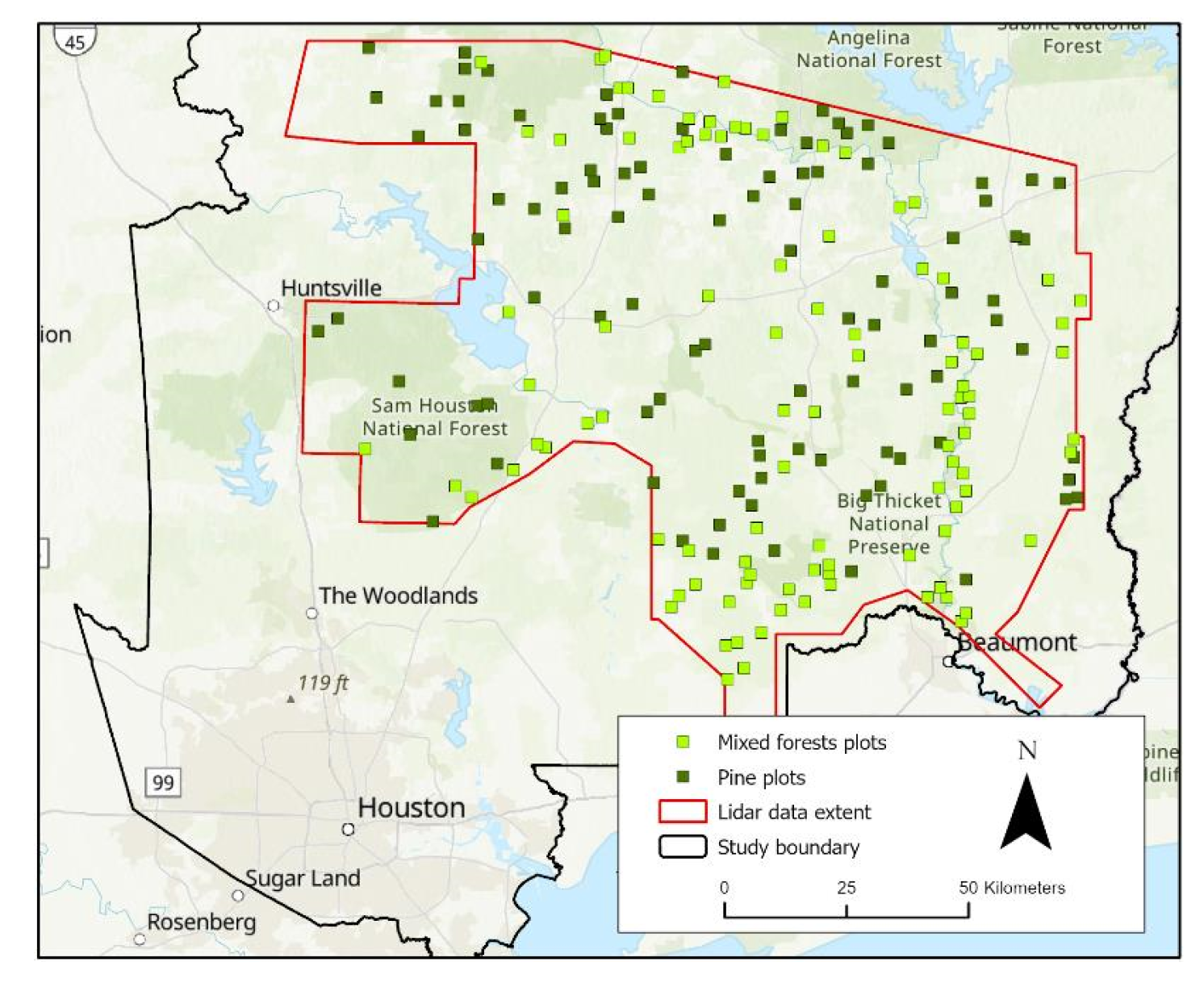
2.1. Study Area

The study area is in southeastern Texas covering an area of approximately 83,300 square kilometers along the Texas–Louisiana border, from the city of Houston to Texarkana on the Texas–Arkansas border (Figure 1). Located largely in the Piney Woods Forest ecoregion, the landscape is dominated by various species of pine trees including Pinus taeda (loblolly pine), Pinus echinata (shortleaf pine) and Pinus elliottii (slash pine), with loblolly pine being the most predominant of the pine species in the region [36]. The region is also home to a variety of hardwoods species including oaks (Quercus stellata (post oak), Quercus alba (white oak), Quercus falcata (southern red oak)) and hickory (Carya texana (black hickory)) [37], with post oaks among the most dominant species. Scattered cropland, planted pastures and native pastures, and suburban and urban areas also occupy a considerable proportion of the study site [36].

2.2. Data

Various datasets were collected to support the development and evaluation of stem volume models including Landsat surface reflectance images, various ancillary data from the LANDFIRE program and plot-level airborne lidar data. Land cover disturbance data were also generated to account for change between the acquisition of airborne lidar data and the Landsat imagery. The following sub-sections describe each dataset collected or generated for this study.

2.2.1. Gap-Filled Landsat Data

Monthly gap-filled Landsat data for January, May and September 2018 were obtained for stem volume modeling and eventual scaling of stem volume estimates to the entire study area. Gap-filled data alleviate the impact of missing image values due to sensor-specific errors and cloud cover [38], which were prevalent across our study area and made obtaining cloud free scenes difficult. The selection of the three months was motivated by the aim to capture different seasons and leaf-on conditions in order to model the impact of phenology on stem modeling. The gap-filled data are derived using the Highly Scalable Temporal Adaptive Reflectance Fusion Model (HISTARFM) algorithm [39], which combines multispectral Landsat 5–8 and MODIS images to reduce noise and produce monthly gap free high resolution (30-m) observations over the contiguous United States. The dataset comprises six wavelength bands including B1 (Blue, 0.45–0.52 µm), B2 (Green, 0.52–0.60 µm), B3 (Red, 0.63–0.69µm), B4 (Near Infrared (NIR), 0.77–0.90 µm), B5 (Shortwave infrared (SWIR) 1, 1.55–1.75 µm) and B7 (SWIR 2, 2.08–2.35 µm). Published quantitative evaluations of the generated products showed highly correlated (R2 > 0.85) and precise (relative mean error below 1.5%) estimates against reference data [39]. Given these high accuracies, we found the gap-filled dataset suitable for application in generating the region-level stem volume dataset.
Figure 1. Study area in eastern Texas, USA. Main map shows the study area classified by ecoregion. The ecoregion classification is based on the RESOLVE Ecoregions 2017 map [40]. The red dashed outline in the main map indicates the extent of airborne lidar data collected for this study. Green star symbols show independent validation sites used to evaluate generated stem volume product. The map inset shows the general location (red rectangular outline) of the study site in the Texas–Louisiana–Arkansas region. Topographic base maps show terrain and river network in both maps courtesy of ESRI ArcGIS®.
Forests 14 00506 g001

2.2.2. LANDFIRE Datasets

Several datasets from the LANDFIRE program for the year 2016 were obtained to serve as additional predictors in the stem volume regression modeling. Below are the listing and brief descriptions of the datasets included:
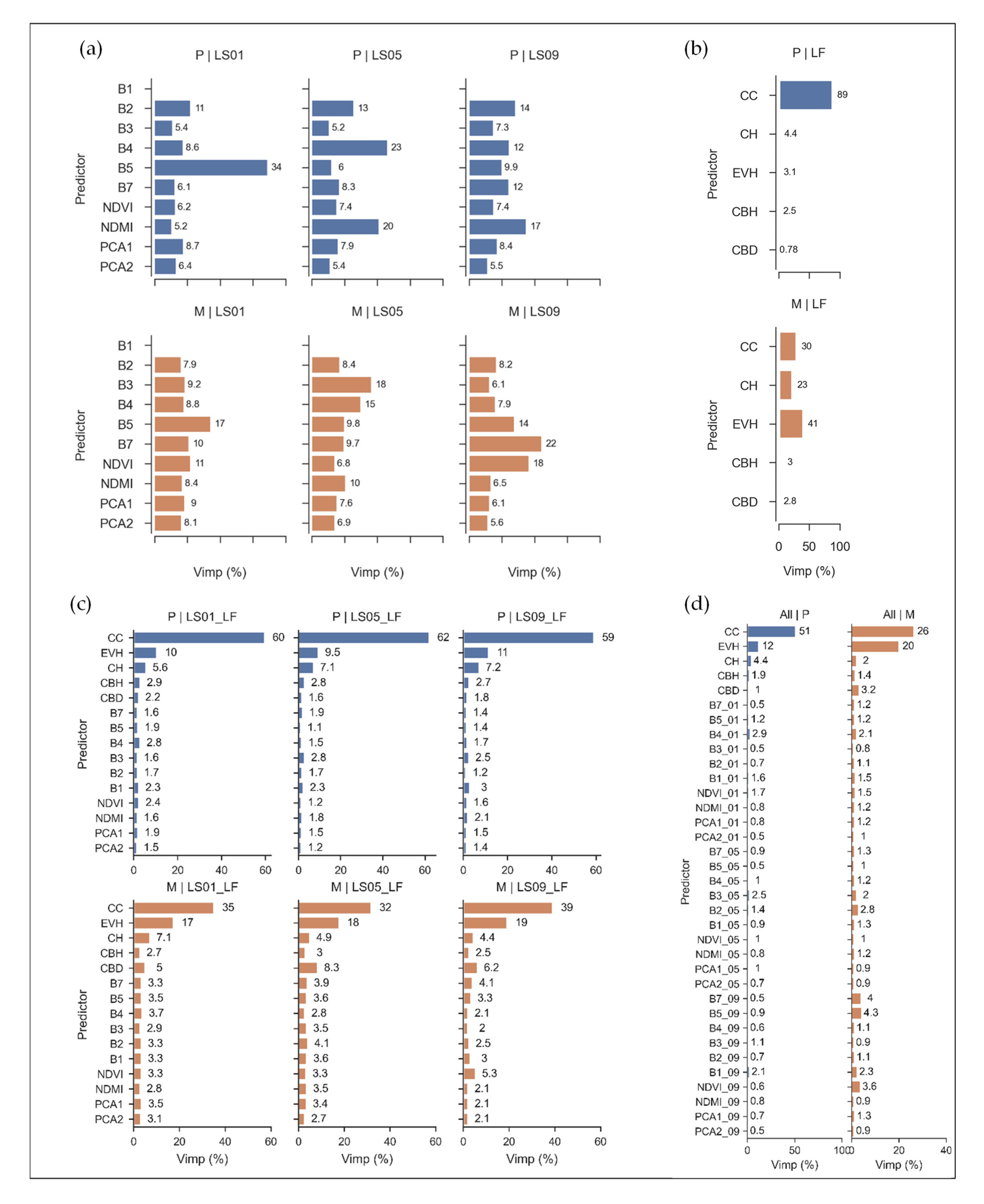
  • Existing Vegetation Height (EVH), which represents the estimated average height of the dominant vegetation for a 30 m grid cell for vegetation lifeforms. EVH values are divided into three distinct ranges depending on lifeform: 0.1 to 1 m with decimeter increments for the herbaceous lifeform, 0.1 to 3 m for the shrub lifeform, and 1 to 99 m in 1 m increments for the tree lifeform.
  • Forest Canopy Height (CH), which represents the estimated average height of the top of the vegetated canopy and is estimated in forested areas only.
  • Forest Canopy Base Height (CBH), which represents the average height from the ground to a forest stand’s canopy bottom.
  • Existing Vegetation Type (EVT) for land cover and species cover information. EVT is meant to represent the current distribution of the terrestrial ecological systems classification. Given that stem volume is dependent on tree species, species cover information was a vital input in generating regional-level products.
  • Forest Canopy Cover (CC) for canopy cover information. CC describes the percent cover of the tree canopy in a stand and is estimated in forested areas only.
  • Forest Canopy Bulk Density (CBD) for ancillary forest structure information. CBD represents the density of available canopy fuel in a stand and is estimated in forested areas only.

2.2.3. Plot-Level Airborne Lidar Data

The use of airborne lidar data allowed for the estimation of tree-level attributes and reference stem volumes. However, since stem volume taper models are usually specific to each tree species and there was a lack of detailed species cover data, the data for airborne lidar were selected based on two broad species groups: (1) pines, which included various pine forests, and (2) mixed forests, which included all deciduous and other wooded forest classes as mapped by the LANDFIRE EVT layer. The airborne lidar data for this study were obtained from OpenTopography, a web portal that facilitates open sharing and access to airborne lidar data globally. The data were acquired between March 2016 and October 2017 under the US Geological Survey (USGS) 3D Elevation Program (3DEP), which is providing the data through OpenTopography [41]. Lidar data over 200 plots (Figure 2), with each plot measuring 330 m by 330 m, were collected across the study area. The ready-classified airborne lidar data had an average point density of 8.87–9.44 points per square meter and was georeferenced to the NAD83(2011), UTM zone 15N reference frame.
The 200 plot locations were determined through a spatially balanced sampling scheme [42]. In spatially balanced sampling, candidate sites are selected based on their calculated inclusion probabilities, which often leads to better spatial distribution of sampled sites over the entire survey area as compared to simple random sampling [43]. To achieve this in this study, a 330 m by 330 m grid was generated over the area of the study site with airborne lidar (Figure 1), designating each grid cell (an 11 by 11 pixel Landsat area), as a sampling unit. For each sampling unit and species type (pines and mixed forests), the percent species coverage was determined based on the recoded EVT data. The percent coverage served as inclusion probability layer for spatially balanced sampling as implemented in the ESRI ArcGIS® software. To ensure high levels of species homogeneity in each selected site, sampling was restricted to sites with percent species coverage above 90% for pines and 85% for mixed forests. For each species group, 100 plots were selected, as shown in Figure 2.
To support independent validation of developed models, another set of 30 (330 m by 330 m) plots, equally divided between pines and mixed forests, was selected and corresponding airborne lidar data collected. Steps were taken to ensure that none of these plots coincided with the 200 plots used for stem volume modeling.

2.2.4. Land Cover Disturbance Data

To account for changes between the acquisition of the airborne lidar data and the Landsat imagery, land cover changes were also mapped over the study site using the LandTrendr (Landsat-based detection of Trends in Disturbance and Recovery) algorithm [44]. LandTrendr automatically extracts information on land surface changes, e.g., deforestation or timber harvesting, and also models recovery processes from a Landsat image time series [29]. LandTrendr applies spectral–temporal segmentation algorithms for change detection in a time series to output the begin and end time of a change event, the change magnitude and duration. In this study, change mapping analyses were based on LandTrendr methods implemented on Google Earth Engine platform. The aim was to minimize the impact of large cover changes on the modeling, thus change parameters in the LandTrendr algorithm were set to capture such changes. Preliminary assessments were performed to determine the optimal change threshold by testing multiple thresholds. A threshold of 300, which represents an increase in the normalized burn ration (NBR) index, was found adequate in capturing known changes, while other input parameters were left at their default levels. For details on all processing parameters, interested readers may refer to the LandTrendr guide or to the relevant publication [44]. Changes were mapped from 2010 to 2019 based on annual Landsat composites. To facilitate filtering of changed areas, the year of disturbance output was recoded into a binary pixel-based layer: 1, for areas that changed since the lidar acquisition in 2016, and 0, for all unchanged areas.

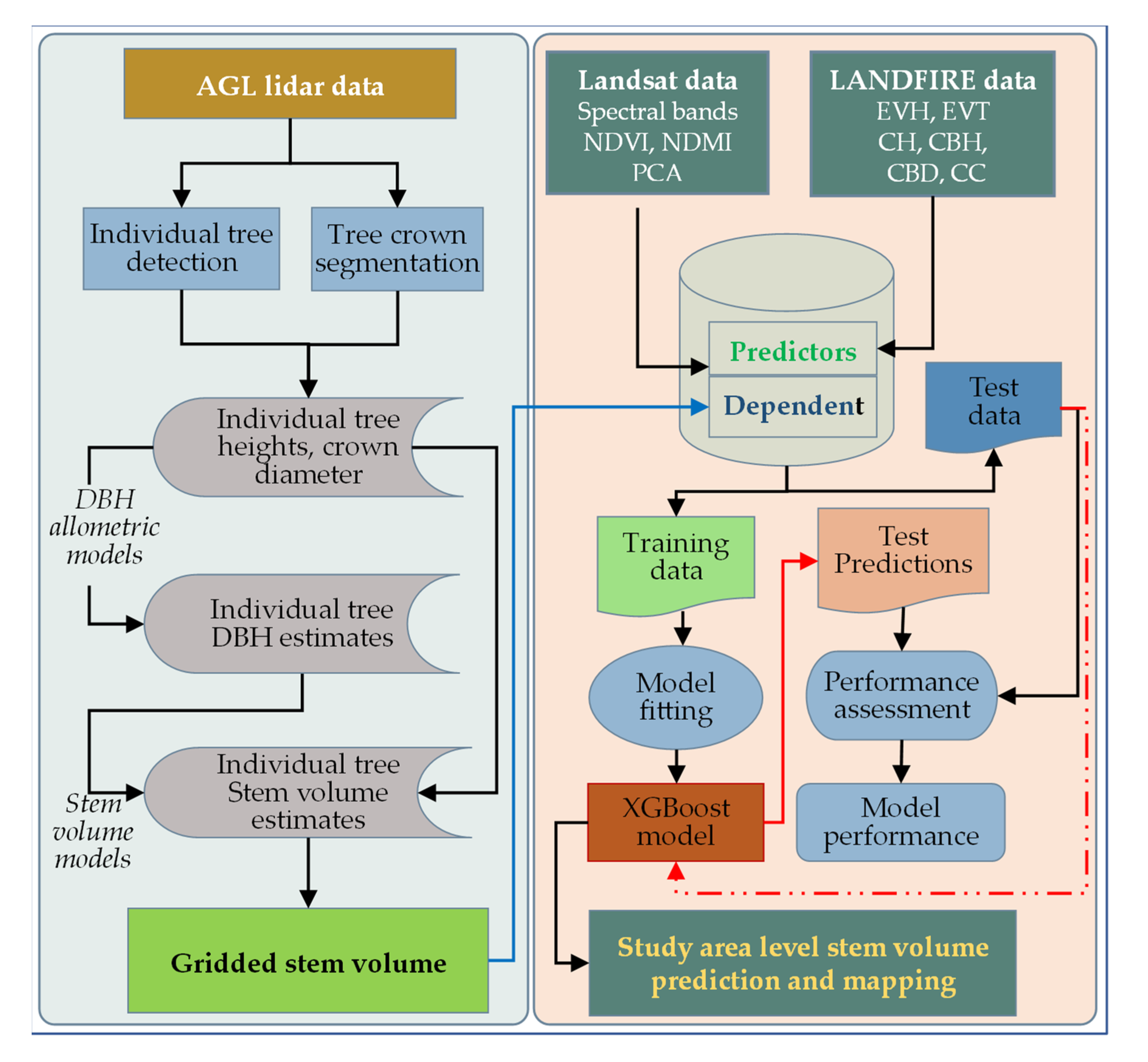
2.3. Data Processing

Figure 3 shows the overall workflow of the processing of the various datasets in this study and the eventual modeling of stem volumes. The following sun-sections highlight individual tree detection and crown segmentation to derive tree-level estimates, use of stem volume allometric models to estimated reference stem volumes and the preprocessing of predictor datasets for stem modeling.

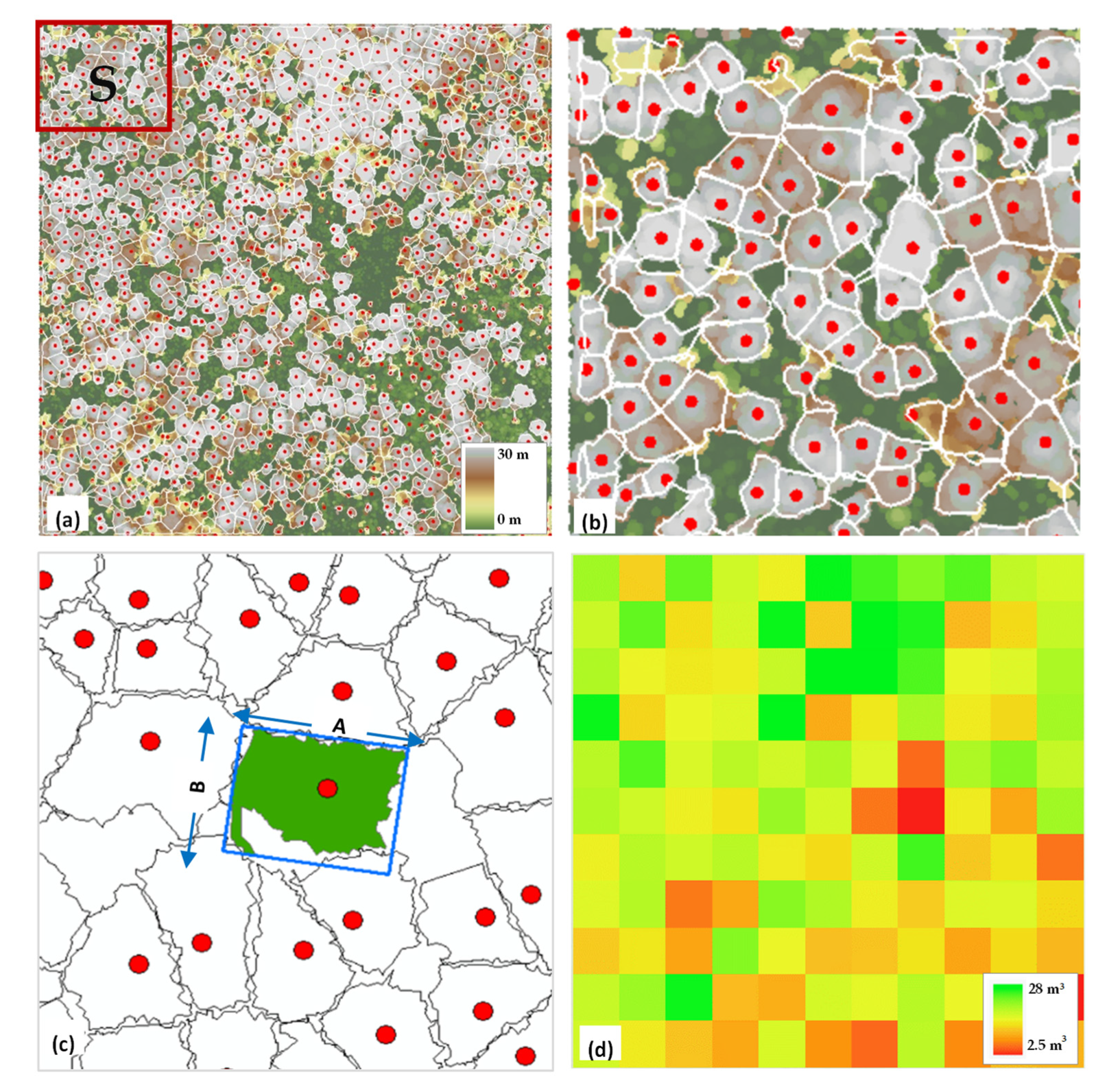
2.3.1. Processing Airborne Lidar Data and Estimation of Tree Attributes

The airborne lidar data for each sampled plot were first preprocessed to remove outliers. To characterize outlying points over the forest canopy, 5 m grid statistics were calculated, and any point that differed by more than 30% from the calculated 95th percentile height statistic was considered outlying and removed. Manual outlier removal was also conducted after the automated outlier removal to ensure all outlying points were removed. Relying on classified ground points, the ground surface was interpolated using the Triangular Interpolation Network method. The point cloud was then normalized to aboveground level to facilitate the detection of individual trees and crown segmentation (Figure 4a). All processing was performed using the lidR package [45], an R package for manipulating and analysis of airborne lidar data for forestry applications.
The method proposed by Popescu and Wynne [46] was applied to automatically locate individual trees in the processed lidar data, while corresponding tree crowns were segmented using a method developed by Silva et al. [47] (Figure 4b), as implemented in the lidR package. The ITD method uses a local variable filtering approach to detect treetops (Figure 4b). A moving window is used to detect peaks in a canopy height model, allowing for adjustment of the window size based on a specified height–crown relationship to detect trees of varying heights. In segmenting tree crowns, the algorithm by Silva et al. [47] uses the detected tree locations, which are buffered based on expected height–crown diameter relationships; finally, a separation of touching crowns is perfirned based on fitting a centroidal Voronoi tessellation.
Prior to applying the ITD and crown segmentation methods to the airborne lidar data, assessments were conducted to determine their performances. The assessments focused on validating the derived number of tree detections, heights and crown diameters based on manual measurements from the airborne lidar data. As the aim of this study was not on design and validation of ITD and crown segmentations, details of the assessments are provided in the Supplementary Materials. The comparison between manual tree locations and automatic tree detections in preliminary investigations showed overall detection rates of 90.6% (n = 276) and 81.4% (n = 163) for pines and mixed forests, respectively. Omission rates were 9.4% and 18.4%, and commission rates were 2.6% and 9.4% for pines and mixed forests, respectively (see Table S1). Outputs of the crown segmentation were assessed based on a selected sample of trees, which were manually measured from the lidar data to determine tree heights and crown diameters (see Table S2). In general, individually detected tree heights were highly correlated with manual tree height measurement ((R2 = 0.98, MAE = 0.34 m for pines, R2 = 0.98, MAE = 0.52 m for mixed forests). Tree crown diameters were moderately correlated (R2 = 0.75, MAE = 0.82 m for pines, R2 = 0.71, MAE = 0.72 m) (Table S3, Figure S1). The level of accuracy achieved in these assessments was considered reasonable and a good basis for regional-level scaling.
The ITD and crown segmentation methods were then applied to derive tree-level attributes (height and crown diameter). In this study, separate height–crown relationships for pines and mixed forests trees were determined for the ITD step based on manual measurements of tree height and crown widths (see Supplementary Materials). Once the trees were detected, the corresponding crowns were segmented. All the sampled lidar data were processed and the detected trees with associated height values exported as a vector layer in shapefile format. Corresponding tree crowns were also saved as a polygon vector layer. From each crown segment, a tree crown diameter was estimated as the average of the length and width of a fitted bounding box, as illustrated in Figure 4c. Alternatively, the crown width could have been estimated as the diagonal length of the fitted bounding box. The average of the dimensions was preferred here to provide a conservative estimate, especially for mal-segmented or elongated crown segments.

2.3.2. Generating Reference Volume Data

Diameter at breast height (DBH) was a key variable in estimating tree-level stem volumes, though it was not directly estimable from airborne lidar data, as earlier stated. Thus, this study relied on published diameter models in Popescu (2007) and Gering and May (1995) to derive DBH estimates for stem volume calculations. The DBH model in Popescu (2007) was applied to the pine species group, while the model in Gering and May (1995) was applied to the mixed forest group. These choices were driven by model goodness-of-fit, similarity of species studied and geographical proximity to this study. Popescu (2007) developed and validated models relating DBH to tree height and crown diameter in loblolly pine trees in eastern Texas based on lidar-derived individual tree measurements and field data. The developed model provided low biases (RMSE = 4.9 cm) and high correlations (R2 = 0.87). Models developed by Gering and May for pine (loblolly/shortleaf) and hardwood (oaks/hickories) species in Tennessee also showed good fit with respect to field measured diameters (R2 = 0.64–0.93, RMSE = 3.86–6.95 cm), providing a good basis for modeling in this study. Given the lidar-derived crown diameter (CD) and tree height H, DBH was estimated per tree according to (1) and (2) for pines and mixed forests, respectively, as follows:
D B H c m = 0.16 + C D + 1.22 H
D B H c m = 1.6961 + 0.4233 C D × 2.54
For (1), measurements of tree height and crown diameter were expressed in meters, while tree measurements in feet were used for (2) to obtain a DBH estimate in centimeters. The 2.54 factor was introduced to convert inches to centimeters from the original equation in Gering and May (1995).
Having estimated the DBH using either (1) or (2), the total stem volume was calculated for each detected tree based on published Forest Inventory and Analysis (FIA) allometric equations (3) and (4) for southern US regions, which includes Texas [6]. The FIA has developed various equations from copious field data to estimate species-specific parameters such as stem volume in cubic feet, which was converted to cubic meter by applying the conversion factor (1 cubic foot = 0.0283 cubic meter). The equations applied here capture total stem volume from ground level to the stem tip. For each species group, separate equations were applied for saplings (DBH > 2.54 cm and < 12.7 cm for pines and hardwoods), poles (DBH ≥ 12.7 cm and < 22.9 cm for pines, DBH ≥ 12.7 cm and < 27.9 cm for hardwoods) and sawtimber (DBH ≥ 22.9 cm for pines, DBH ≥ 27.9 cm for hardwoods), as follows:
V j = k × C V 4 j ;     j = s a p l i n g k × T F j × C V 4 j ;     j = p o l e , s a w t i m b e r
C V 4 j = a 1 j + a 2 j × D 2 × H T F j = b 1 j + b 2 j × D 2 × H
where D = DBH, inches; H = total height, meter; k is a cubic foot to cubic meter conversion factor (0.0283); and a1j, a2j, b1j and b2j are separate coefficients for sapling, poles and sawtimber in each species group (Table 1). CV4 represents volume of 1-foot (~0.31 m) stump to a 4-inch (~10.2 cm) top diameter outside bark diameter, while TF represents the total volume from ground to tip. The estimation of stem volume was modeled after dominant species model coefficients. For the pine group, coefficients for loblolly pine were used, while coefficients for post oak were applied for mixed forest group. To match the Landsat image spatial resolution, all per-tree stem volume estimates from each plot were then aggregated at a 30 m scale by summing all tree-level volume estimates in each 30 m pixel (Figure 4d).

2.3.3. Preprocessing and Combining Predictor Variables

All the collected Landsat images were clipped to study area extent and geolocated to a common reference frame (WGS84 UTM zone 15N). Additional predictors including spectral indices and principal components were generated from the raw images. Two spectral indices were calculated, having shown better correlation with stem volumes in preliminary analyses: the normalized difference vegetation index (NDVI) and the normalized difference moisture index (NDMI) [48], and are written according to (5) and (6), respectively, as the following:
N D V I = B 4 B 3 B 4 + B 3
N D M I = B 4 B 5 B 4 + B 5
where B3, B4 and B5 represent Band 3, Band 4 and Band 5, respectively, as stated in Section 2.2.2. Principal component analysis (PCA) bands were also generated for each Landsat scene but only the first two component bands were used since they accounted for almost all (above 95%) the variability in the data.
All LANDFIRE datasets were projected to WGS84 UTM zone 15N and clipped to the study area extent. For storage and ease of data management, LANDFIRE datasets that capture continuous values such as height are encoded as ordinal values that are proportional to actual values. For instance, EVH for the tree lifeform category is encoded with values from 101 to 199 where 101 represents 1 m, 102 represents 2 m and so forth. Thus, for modeling purposes, these values were applied without recoding them to their actual values. This applied to EVH, CH, CBH, CBD and CC. As stated earlier, two broad species groups were considered for modeling purposes given the coarse species cover data over the study area. Thus, the EVT data were recoded into three broad categories based on national vegetation classification attribute data: (1) pines, which included all pines forests (loblolly, shortleaf and longleaf), (2) mixed forests, which included the deciduous, mixed and woody wetlands classes and (3) non-forest, for all other herbaceous vegetation, non-vegetated classes (developed areas) and open water. This data categorization enabled development of separate volume models for pine and mixed forests.
Having processed all the predictor variables and generated the gridded reference stem volumes in all plots, all these data were stacked together to create an image dataset for stem volume modeling. Further, the dataset was reformatted as a table and all observations in changed areas removed.

2.4. Stem Volume Modeling

2.4.1. XGBoost Model Building and Assessment

XGBoost, for Extreme Gradient Boosting, is an optimized distributed gradient boosting library which provides a parallel tree boosting to solve both classification and regression problems in a fast and accurate way [49]. By building sequential decision trees that are incrementally improved, gradient-boosted trees as implemented in XGBoost can learn the complex nonlinear relationships that occur between predictors and output dependent variables. Being a non-parametric model, XGBoost was also preferable given the correlated predictors from Landsat and LANDFIRE. In preliminary analyses in which the purpose was to select a regression approach for modeling stem volume in this study, other algorithms were evaluated including random forests and deep neural networks [50]. Models based on XGBoost showed better performance compared to the other two methods; thus, XGBoost was adopted as the main method for this study.
As with any machine learning model, the performance of XGBoost is dependent on predictors used and the set of model parameters (hyperparameters) specified during training. In this study, LANDFIRE, Landsat surface reflectance imagery, principal components and spectral index predictors were evaluated to improve the effectiveness of developed models. Apart from selecting appropriate features, it was also critical to find optimal values for several hyperparameters used in the model. The hyperparameter tuning step is vital to build models with high performance and models that can generalize well when applied to test data. With XGBoost, parameters tuned included the number of decision trees, number of features when splitting, the learning rate and several other parameters that control data splitting and regularization. Optimal model parameters were determined through an exhaustive grid search approach [51]. Grid search exhaustively evaluates all parameter combinations from the parameter space to determine the best combination of parameter values for building the model.
Regression models were set up using XGBoost, taking the gridded stem volume data as the dependent variable and the Landsat images, Landsat spectral indices and principal components, and LANDFIRE data as predictors. The modeling was performed by species group, taking a 30 m pixel as a sampling unit. Several modeling scenarios were evaluated to assess the impact or benefit of (1) Landsat imagery acquired at separate times and (2) combining multitemporal Landsat data. Thus, models were developed as follows:
  • Separate models were built using LANDFIRE data only and using each of three Landsat 8 images.
  • Combined models were built using LANDFIRE with each of the Landsat images. A combined model was also built by combining all the LANDFIRE and Landsat 8 data regardless of acquisition date to assess the benefit of using all the multitemporal Landsat data.
For each of the models, 85% of the data (pixels from 85 subsites in each case) including all pixels in samples sites were used for training and 15% for evaluating the accuracy of the prediction. The performance of the models was evaluated based on mean bias (Bias), mean absolute error (MAE) and their equivalent percent metrics, percent bias (pBias) and percent MAE (pMAE), as shown in Equations (7) through (10), where Volpred is the predicted total stem volume, Volref is the reference total stem volume and n is the total number of samples used for the assessment. Given the reference is subtracted from the predicted stem volume in the above bias metrics, a negative value indicates general underestimation of reference stem volumes and vice versa. MAE was applied to assess the precision of the predictions with respect to reference stem volumes. To assess the correlation between predictions and reference stem volume estimates, the coefficient of determination (R2) was also calculated. For each fitted model, variable importance was assessed as the average gain across all splits where a variable was used in the decision trees. Thus, the variable importance value captures the relative contribution of a particular variable to model performance—a higher value shows higher importance in predicting target values.
B i a s = 1 n i = 1 n V o l p r e d V o l r e f
p B i a s = 100 × i = 1 n V o l p r e d V o l r e f i = 1 n V o l r e f
M A E = 1 n i = 1 n V o l p r e d V o l r e f
p M A E = 100 × i = 1 n V o l p r e d V o l r e f i = 1 n V o l r e f

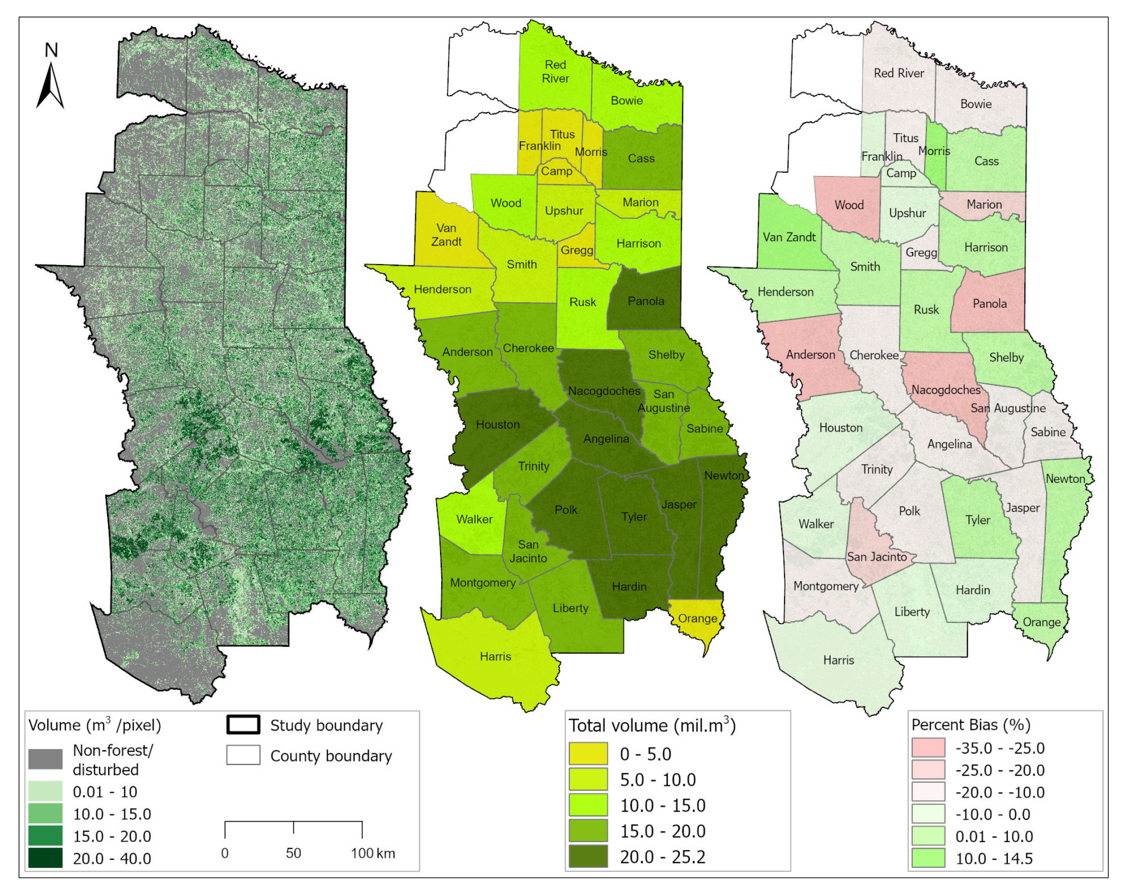
2.4.2. Generating and Validating the Regional Stem Volume Product

The stem volume product was generated by applying the developed regression models to the gap-filled Landsat [39] and LANDFIRE data over the entire study area in eastern Texas. Essentially, the generated product represented total stem volume in each Landsat pixel. Based on the recoded EVT data, pixels with a value of 1 were processed using the developed pine regression model while pixels with the value of 2 were processed with the mixed hardwood regression model. Non-forest (Barren class) and changed pixels according to the disturbance data were omitted from the model predictions and assigned a value to of zero.
Comparative assessments were carried between the generated stem volume product and reference stem volume estimates using two sources of reference stem volume data:
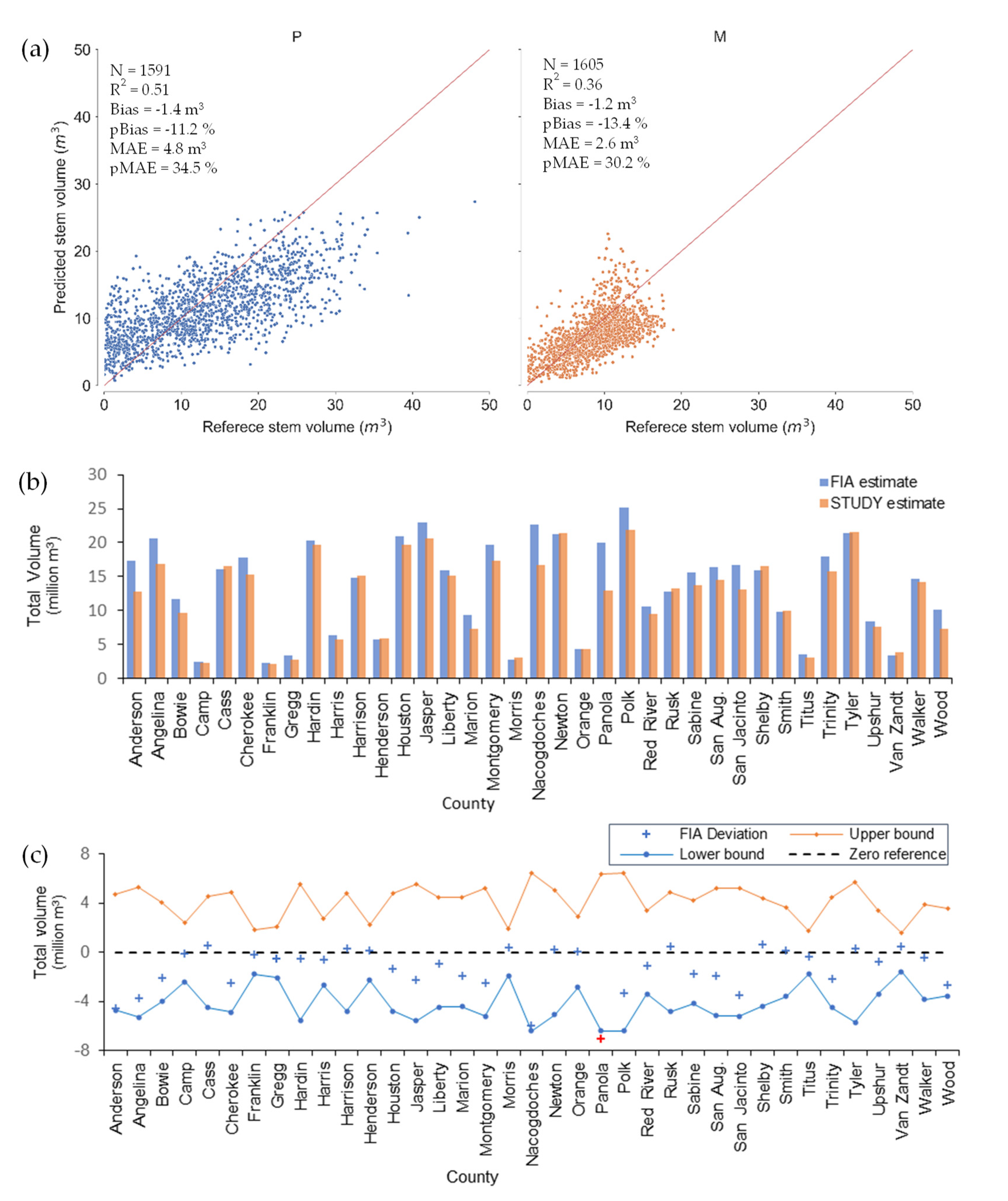
  • First, airborne lidar data from the 30 independent sites (Section 2.2.3, Figure 1) were used to derived stem volume estimates following methods in Section 2.3.1 and Section 2.3.2. The derived reference stem volume estimates were compared to matching estimates from the generated stem volume product using metrics in Section 2.4.1.
  • Second, comparative assessments were conducted against existing FIA county-level stem volume estimates to determine the agreement between the two products. County-level stem volume estimates were derived from the FIA Landcover County Estimates 2017 dataset [52], which represents forest area estimates and associated percent sampling error by county generated from the Forest FIA inventory measurements for the year 2017. Data for 2017 were used because of the closeness in time to both the airborne lidar acquisition and the LANDFIRE release dates. The generated stem volume product was aggregated at the county level, and totals were compared to FIA county estimates to facilitate the comparison. The FIA County stem volume estimates compared were the net merchantable bole volume of live trees with at least 12.7 cm DBH on forest land. Again, evaluation metrics in Section 2.4.1 were used to assess the agreement between the two products. A further evaluation of the two products was conducted based on the percent sampling error included in the FIA data, which represent a standard deviation estimate for each per-county volume estimates. These error data were used in this study to construct per-county 95% confidence intervals to provide a graphical view of which of the study-county stem volume estimates fell within the FIA confidence interval.

3. Results

3.1. Stem Modeling with Landsat and LANDFIRE Data

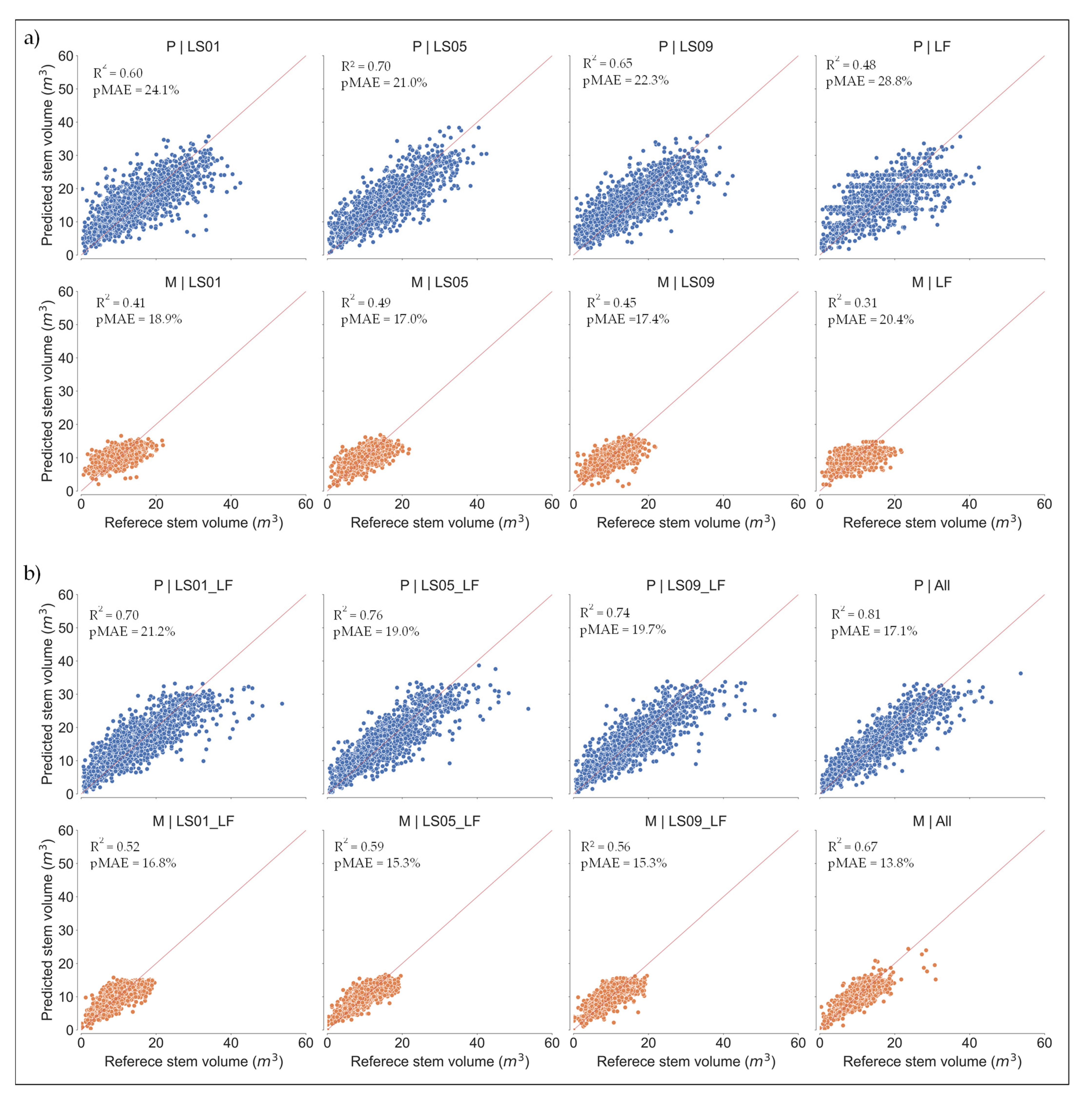
3.1.1. Model Performance with Separate Landsat and LANDFIRE Data

Table 2 and Figure 5a summarize the performance of models fit with separate Landsat and LANDFIRE predictors. Overall, R2 values varied from 0.36 to 0.70 and from 0.19 to 0.49 for pines and mixed forests, respectively. The best performance in each case was observed when applying the full set of May Landsat predictors, which included all Landsat bands, spectral indices and PCA bands. In general, reference stem volume estimates were overestimated for both pine (average Bias 0.2 m3) and mixed (average Bias 0.01 m3) forests. Predicted stem volumes were on average within 26.3% and 19.2% of reference values in pines and mixed forests, respectively. The full set of Landsat based predictors provided better predictions (average R2 = 0.65, MAE = 3.5 m3 for pines, average R2 = 0.45, MAE = 1.9 m3 for mixed forests) than a set of LANDFIRE predictors (R2 = 0.48, MAE = 4.4 m3 for pines, R2 = 0.31, MAE = 2.2 m3 for mixed forests). While this observation might reflect the quality of predictors used, it must be interpreted in the context of the number of predictors involved (10 Landsat versus 5 LANDFIRE), as regression model fits usually improve with a higher number of predictors. In fact, when only the best five Landsat-based predictors were used in the modeling to match the number of LANDFIRE predictors, the performance drastically reduced to within LANDFIRE performance levels (Table 1). Thus, based on an equal number of predictors, Landsat- and LANDFIRE-based predictors showed similar performance in the stem modeling.

3.1.2. Model Performance with Combined Landsat and LANDFIRE Data

Table 3 summarizes the performance of the four regression models trained for predicting stem volume when combinations of Landsat and LANDFIRE predictors were applied. For both species groups, R2 values ranged from 0.52 to 0.81, indicating moderate-to-high correlation with respect to reference stem volume estimates. Mean bias values ranged from −0.12 m3 (under-estimation) to 1.2 m3 (overestimation), which translated to relative percent biases of −1.1% to 1.2%. MAE values ranged from 1.5 to 3.3 m3, representing relative deviation from reference stem values of 13.8 to 21.2%. These evaluation metrics show that the XGBoost models developed with both Landsat and LANDFIRE predictors performed better both in terms of the correlation (12.8% average improvement in R2 for pines, 24.7% for mixed forests) and precision (9.6% average improvement in MAE for pines, 8.9% for mixed forests) of stem volume predictions.
As in the previous section, model performance in pine forests varied by the Landsat date, with the model trained with LANDFIRE and May Landsat data showing the best performance among separate models in terms of R2, Bias and MAE values (Table 3, Figure 5b). The second-best performance was observed using LANDFIRE and September Landsat data, with the models developed with January Landsat data showing the lowest performance. All models fit for pine forests showed a level of overestimation (Bias 0.02–0.18 m3) with respect to reference stem volume values. All models also showed good precision, reaching to within 20% of reference values. Model performance in mixed forests varied in a similar way as pine forests, with performance better for models fitted with May and September Landsat images than with the January Landsat image. As with the models fitted with separate Landsat or LANDIRE, the significant difference between the two cases (pines and mixed forests) lay in the level of performance. In the mixed forests, the observed R2 values (0.52–0.59) were lower than the pine case (0.70–0.76), which amounted on average to a 24% decrease. The mean bias magnitudes for mixed hardwood forest were comparable to pine forest, except for the fact that general underestimation was observed (pBias = −1.1–−0.4%). However, models for mixed forest showed better precision (pMAE = 15.3–16.8 %) compared to pine forests (pMAE = 19–21.2%).
When all the LANDFIRE and Landsat predictors from the three dates were included in the stem volume regression model, model performance improved further across metrics. In terms of correlation, the R2 value for pines increased to 0.81 while the R2 value for mixed forests rose to 0.67, representing improvements of 9.1% and 20.4% respectively. Models fitted with combined data were on average less biased (pBias = 0.3% for pines, pBias = −0.2% for mixed forests), although individual models fitted with Landsat data for 05/2018 and 09/2018 showed better mean biases. Precision with respect to reference stem volume estimates also improved (average pMAE improvement of 2.86% for pines and average pMAE improvement of 2.0% for mixed hardwoods), but was less significant compared to gains in R2 values. These results demonstrate a further benefit in combining multitemporal imagery and multisource data in stem volume modeling.

3.1.3. Model Variable Importance

Variable importance scores from models fitted with separate and combined Landsat and LANDIRE predictors varied by species group and, for Landsat, by acquisition date (Figure 6). Separate Landsat models fit for pines and mixed forests showed a dominance of features from red, near-infrared and shortwave-infrared spectra (Figure 6a). The three top-ranked pines were Bands 3 and 4 and NDMI, while Band 7, Band 4 and NDVI were the most important in mixed forests (refer to Section 2.2. for band information). It is worth noting that the three top-ranked predictors accounted for less than 60%, indicating the importance of the other predictors to overall model performance (Figure 6a), implying that the remaining features were still critical for adequate model performance. In general, individual Landsat bands and spectral indices were ranked higher than PCA bands. Variable importance scores for LANDFIRE predictors showed a more lop-sided contribution to model performance, with over 90% attributed to top three predictors (CC, EVH, CH). CC accounted for most of the variable importance (89.2%) for pine models, but a more even distribution among the three variables was observed for mixed forest models.
Models developed with combined predictors showed LANDFIRE predictors were ranked higher than Landsat-derived predictors. The CC predictor was the highest-ranked predictor followed by EVH across all scenarios. For models developed for pine forests, the CC predictor accounted for about 60% of the variable importance but was reduced to about 35% for mixed hardwood forests, where the loss in importance was driven by gains by other predictors, especially EVH. The higher performance of CC as compared to EVH and CH in the stem regression models was unexpected given that the other predictors (EVH and CH) were seen to have a more direct involvement in the computation of stem volume. Equally unexpected was the better performance of EVH over CH. Variable importance ranking for CBH and CBD varied across forest type, with CBH showing a higher contribution to model performance in pine forests, whereas CBD showed a higher performance in mixed hardwood forests. Similar to models developed with separate Landsat predictors, the variable importance ranking for Landsat-derived predictors fluctuated across forest type and over the three dates. Landsat Band 1, 3 and 4 were among the highly ranked predictors in pine forests, and spectral index predictors (NDVI and NDMI) were generally ranked higher than the two principal components across the three dates. In mixed hardwood forests, Landsat Band 2, 5 and 7 showed higher ranking in general. In this case, NDVI was more important than most of the individual Landsat bands. Again, principal components did not rank higher than spectral indices and individual bands.
Combining all predictors regardless of acquisition dates revealed interesting patterns. For models over pine forests, the top-three highly ranked Landsat predictors (band4_01, band3_05 and band2_09) were shared among the three dates. However, for models over mixed hardwood forests, the highly ranked Landsat predictors (band5_09, band7_09 and ndvi_09) all came from the 09/2018 image. These observations point to different seasons for optimally mapping the two forest types. As in other modeling scenarios, LANDFIRE predictors still ranked higher than Landsat predictors, although at a lower level than in separate models.

3.2. Stem Volume Product Generation and Comparison with Reference Products

Figure 7 (left) shows the stem volume map generated over the entire study area in eastern Texas. Stem volume ranged from 0 to 42.5 m3 per 30 m pixel with the variation conforming mainly to the spatial patterns of forests over the region. Higher stem volumes are concentrated mainly in the southern part of the study site around national forests dominated by pine and hardwood species. In the northern part of the region, there were lower stem volume values owing to the change in ecoregion from a more densely forested Piney Woods to moderate-to-sparse East Central Texas forests (Figure 1). Figure 7 (middle) shows FIA county-level stem volume map over the study area. Albeit for the different spatial scales, the gradation in total per-county stem volumes is reflective of the stem volume generated in this study. Quantitatively, the two products differed, with their county-level differences showing varying levels of under and overestimation (Figure 7, right).
Comparison of the stem volume estimates from the generated product with independent airborne lidar-derived stem volume estimates showed moderate correlations (R2 = 0.51) and higher biases (pBias = −12.2%) compared to results based on hold-out data (Section 3.1.2). Figure 8a shows scatterplots with performance metrics of the comparison between stem volume estimates from the generated product and independent estimates derived from airborne lidar data in sample sites. Estimates from pine sites showed R2 value of 0.51 with percent biases of −11.2%, which showed a loss of predictive performance. Estimates from mixed forests showed also showed reduced agreement (R2 = 0.36, pBias = −13.4%) over hold-out test data. The reduction in predictive performance on independent estimates is somewhat expected, and is indicative of some inadequacies in sampling and predictor inefficiency in capturing the full range of forest stem volumes.
On the other hand, the comparison of aggregated per-county stem volumes estimates with FIA estimates showed a high linear correlation (R2 = 0.93) between the two datasets, showing the consistency of the approach applied in this study Figure 8b). In terms of bias, our stem volume estimates underestimated (pBias = −10.3%, pMAE = 11.7%) corresponding FIA stem volume estimates. The general underestimation is in line with results from independent sites. An assessment of study’s stem volume estimates with respect to 95% confidence intervals calculated from the FIA percent sampling error showed that the majority (97.3%) of the county-level stem volume estimates were within expected error range. The only estimate that was not within the 95% confidence interval is from Panola County. Given that other estimates from counties farther from the airborne lidar sampling (Figure 7, right; Figure 8c) agreed with FIA estimates, factors other than distance could have influenced our modeling. On the whole, these results are promising given that FIA estimates are based on detailed unbiased tree estimates from a network of FIA plots, while the approach applied here was based on individual tree detections, which may not detect some understory trees.

4. Discussion

The goal of this study was to develop and evaluate methods for creating spatially detailed regional maps of stem volume, which could support resource management and be widely accessible beyond county-level datasets. To achieve this, this study leveraged multisource data to scale estimates of tree-level stem volume to a regional level at a 30 m Landsat spatial resolution. The consistency in spatial resolution between the Landsat and LANDFIRE datasets made the scaling process easier and eliminated the need for additional resampling processing steps. The regression models developed in this study provided moderate to highly correlated predictions, with R2 values ranging from 0.52 to 0.81. The predictions were virtually unbiased, with pBias values ranging from −1.1% to 1.2%, and precise, with pMAE values ranging from 13.8% to 21.2%, when compared to reference stem volume estimates. These results demonstrated the effectiveness of the multisource approach used in this study, which benefitted from the effective and robust gradient-boosted trees regression algorithm [50] and the multisource predictors.
This study’s tree-to-regional-level scaling approach also performed comparatively well when compared against independent airborne lidar-derived estimates (R2 = 0.51, pBias = −12.1%, pMAE = 32.1%). It also performed well when compared to existing FIA county-level stem volume estimates (R2 = 0.93, pBias =−10.3%, pMAE = 11.7%). Furthermore, all but one of the county-level stem volume estimates were within the FIA 95% confidence intervals, showing adequate reliability of ITD approach for modeling forest stem volume at regional levels. However, in contrast to the FIA county-level dataset, the maps produced in this study provide a more comprehensive and detailed view of stem volume over a larger area. This would enable resource managers to better identify areas for timber harvest, carbon accounting and ecological process assessments.
Several previous studies have reported a wide range of error values in estimating stem volumes in various forest ecoregions. Magnusson and Fransson (2005) used a non-parametric regression K-nearest neighbor approach to estimate the stand volume for coniferous stands in Sweden using combinations of SPOT, Landsat and stand-level tree height data, and reported estimation root mean square errors (RMSE) between 11.2% and 25.2%. The best model performance (11.2%) was achieved by inclusion of field-measured stand-level tree heights as compared to image data alone. Hyyppä et al. (2000) assessed the accuracy of estimating stem volume over a boreal forest test site using various remote sensing datasets including aerial photographs, Landsat TM, SPOT and various SAR datasets (airborne ranging radar, European Remote Sensing satellite (ERS), Japanese Earth Resources Satellite 1). The models developed with the various datasets showed R2 values between 0.06 and 0.68 and RMSE percentages between 34 and 65%. Interestingly, predictors derived from optical images provided more predictive power for forest inventory than SAR intensity and coherence-based predictors, except for radar profiles, which the authors attributed to the significant decrease in coherence between acquisitions. These studies highlight the vital importance of non-spectral predictors, e.g., stand-level tree heights and radar profiles, with more considerable correlation with forest structure to modeling forest structural parameters such as stem volume. In this study, prior estimates of tree height and other structural parameters from the LANDFIRE datasets were used to achieve this goal. Using a variety of predictors including Landsat 7 reflectance bands, vegetation indices and textures features, [14] reported RMSE error percentages between 30% and 40% in estimating stem volume in Indonesia. Although field measurements were utilized in this study, their margins of error were not superior to the ITD approach employed here. This could be attributed to the fact that their approach relied on traditional multiple regression modeling instead of the more robust gradient-boosted trees used in this study. The performance of Sentinel-2 and Landsat 8 for estimating forest volume in a boreal forest in Southern Finland was carried out by [33]. Sentinel-2 data provided better estimates (RMSE = 59.3%) than Landsat (RMSE = 72.2%), which the authors attributed to Sentinel-2′s red-edge bands and better spatial resolution. The high errors reported by the study again underscore the need to include other multisource datasets to improve predictive performance. Similar to this study, [53] used multi-year Landsat and spectral index time series to estimate the stem volume of six Canadian sites, achieving errors ranging between 20 and 60%, which was attributed to site-specific structure differences. Like [14], this study relied on plot-levels field measurements, and was limited to optimizing the time-series length over the six site as opposed to an actual large-scale mapping of forest volume. Compared to these previous studies, this study achieved model percent RMSE values between 18.6 and 45.9% (Table A1, Appendix A), which shows improvement over the previous studies, especially considering the regional-scale stem volume product generated. Overall, the level of accuracy in this study and previous studies show the critical importance of multisource predictors in characterizing forest structural parameters, but also underscore the difficulty of estimating forest parameters with reduced uncertainty.
While Landsat data is a major input in the generation of LANDFIRE products, it was still useful to take advantage of the varying spectral responses of different bands to forest condition and structure to support modeling. The benefit of using multitemporal Landsat data was demonstrated by the better observed model performance when combined Landsat data were used. The use of data at multiple dates also reflected the influence of phenology on the retrieval of forest stem volume, with models based on leaf-on data (05/2018, 09/2018) showing higher performance compared to a model based on leaf-off data. Interestingly, higher gains (20.4 vs. 9.1 %, Section 3.1.2) were observed for mixed forests than pines when combined data were used, reflecting a prediction boost from phenological changes associated with mixed forests than evergreen pines. These observations are in line with previous studies that have shown the importance of applying multitemporal data in both stem volume and biomass modeling [53,54,55]. Despite using multitemporal Landsat data, LANDFIRE variables contributed more predictive power than predictors derived from Landsat data in combined models, which was expected given the more direct relationship of variables such as EVH to stem volume. Though not directly related to the computation of stem volume, CC showed higher variable importance across modeling scenarios due to its relationship with stand density [56,57]. However, it is worth noting that LANDFIRE as a modeled product has shortcomings in accurately characterizing forest structure. This likely explains the underestimation of stem volumes as shown in Figure 5. Fitted models were only able to estimate up to 36.8 m3 and 17.0 m3 compared to maximum reference values of over 42.5 and 19.8 m3 for pine and mixed forests, respectively.
Model performance varied by species group, with pine-based models showing better correlation and overall biases compared to models for mixed forests. These results are attributable to a number of factors including differences in performance of the ITD and crown segmentation and the level of generality in applied allometric models. The ITD method applied here showed lower performance in mixed (81.4% accuracy) compared to pine forests (90.6% accuracy), a pattern observed in previous studies that assessed ITD performance in both coniferous and deciduous [46,58]. The higher accuracy in pines is attributed to their simpler conical shapes, which are amenable to easier detection compared to deciduous trees that tend to show fewer dominant peaks. Further omission could also be attributed to poor detection of co-dominant and understory trees, which most ITD methods struggle with [59,60]. Apart from uncertainty in detection, methods applied here also showed a level of uncertainty in estimating tree-level attributes such as tree height and crown diameter (Supplementary Materials). The errors associated with these attributes propagated the estimation of DBH, which later affected the resulting stem volume. It is noteworthy to outline the implications on the DBH model parameterization. The pine DBH model required both the tree height and crown diameter to be estimated, while the one for the mixed forest only required one. Considering the similar level of precision in estimating crown diameter, higher uncertainty can be expected from the model with two parameters. This could partly explain the higher precision obtained in mixed forests as compared to pines. In the two cases studied, stem volume was modeled based on stem volume taper models for a dominant species, which has implications on the level of generality of the allometric models. The pine group performed better than the mixed forest due to the dominance of loblolly pines in the study area; considering the similar stem morphology of other pine species, this led to higher consistency in modeling based on allometric equations from a single species than more diverse mixed forest group. This, together with the limitations in ITD methods, led to the observed prediction trends in the two cases.
The modeling framework presented here complements previous efforts [1,12,24] aimed at consistent modeling and monitoring of stem volumes and forest biomass across regional and global scales. For the US, where LANDFIRE datasets are available on a national scale under a consistent processing methodology, the methods developed in this study could readily support extended modeling to cover other areas across the US. The methods presented here are also adaptable to other regions outside the US. LANDFIRE datasets used in this study characterized aspects of canopy cover, canopy height and land cover of which suitable alternatives can be found at national and global levels. Notable alternatives include datasets being generated under the Copernicus program [61] and global datasets generated by NASA such as the global forest cover datasets [26] and tree height [28,62]. The key factor in using all these multisource datasets is accounting for changes as conducted in this study. Models fit with Landsat-only predictors also showed competitive performance, indicating that the methodology applied here could be used without additional ancillary predictors. Other potential applications of the methology presented here include the assessment of stem volume in multiple years, providing opportunities to monitor status and trends in forest resources. This modeling framework also offers possibilities for regional monitoring of carbon stocks based on established scaling mechanisms such as applying expansion factors in the component ratio approach [1]. Through such mechanisms, generated stem volume data could be readily converted to forest carbon to support climate mitigation initiatives and carbon accounting initiatives such as REDD+.
There is still a need for continued development in methods and datasets to reduce uncertainties in modeling forest parameters such as stem volume. Much progress has been made in the development of individual tree detection and crown segmentation methods, which are enabling retrieval of tree-level metrics. However, our ability to map tree species at a similar scale still lags. This limitation may be attributable to the lack of widely available high-spatial-resolution multispectral or hyperspectral imagery over large areas to support discrimination of tree species. The lack of detailed species information limits application of species specific allometric equations even though allometric equations for numerous species are available [6]. A few opportunities exist for producing detailed species datasets including national level datasets from the National Agricultural Imagery Program (NAIP) and high-resolution imagery from unmanned aerial systems. NAIP imagery has shown potential for high-resolution species mapping [63,64]. However, with a 1 m resolution, limited spectral bands and infrequent or snapshot collection may still be limited in discriminating individual trees species. Unmanned aerial systems are revolutionizing the collection of various high-resolution remote sensing data, and present another promising option for detailed species classification. Coupled with robust and high-performance approaches such as deep learning approaches, UAS image data could lead to tremendous improvement in land cover characterization at local scales [65]. With such robust methods and high-resolution imagery, it is conceivable that the gap between stand-level and regional-level characterization of stem volumes could be reduced as such data become available over large areas.

5. Conclusions

This study aimed to develop and evaluate stem volume regression models using LANDFIRE and Landsat variables, generate a regional stem volume product by scaling reference stem volumes using the developed models and assess model performance by comparing estimated volumes with independent reference stem volume estimates. The developed regression models showed adequate consistency and precision when compared to reference stem volume estimates, and demonstrated the added benefit of using multitemporal rather than a single-date Landsat image for the estimation of forest stem volume. While the use of ground measurements is still recommended, the results from this study show that there is high potential for developing adequately precise regional products by leveraging automatically derived tree measurements from airborne lidar and ancillary datasets.
Modeling performance varied by species group, with pine-based models showing better correlation and overall biases compared to models for mixed forests. The wide variety of tree species under the mixed forest was much harder to model with a single allometric relationship than pines that tend to exhibit similar shapes. More detailed species cover maps will be required if we are to make full use of the numerous stem volume equations and match outputs from ITD methods. However, for regional mapping, broad species modeling as applied in this study still provides vital spatial information on the status and distribution of forest resources.
Other factors that impacted performance include errors due the individual tree detection and crown segmentation, errors in derived datasets from LANDFIRE, sub-optimal sampling of plots and seasonal changes in vegetation structure as shown by the different performances with leaf-on and leaf-off Landsat data. Future studies should pay attention to these error sources for optimal modeling and scaling of plot-level estimates to regional scales.
Overall, this study provides important insights into developing and evaluating stem volume regression models and offers a useful framework for generating regional stem volume products and assessing model performance.

Supplementary Materials

The following are available online at https://www.mdpi.com/article/10.3390/f14030506/s1, Figure S1: Estimated versus measured tree height and crown diameter for pines and mixed forests, Table S1: Summary of tree detections and associated accuracies, Table S2: Measured (Meas.) and estimated (Est.) tree heights and crown diameters (CD)for randomly selected trees for pines and mixed forests. Unmatched trees not detected or segmented were removed reducing the sample from 30 in each case, Table S3: Assessment of estimated tree height and crown diameter for pines (N = 29) and mixed (N = 20) forests. References [66,67,68] are cited in the Supplementary Materials.

Author Contributions

Conceptualization, L.M. and S.C.P.; Data curation, L.M. and N.-W.K.; Formal analysis, L.M.; Funding acquisition, L.M. and S.C.P.; Investigation, L.M.; Methodology, L.M.; Project administration, S.C.P., J.R. and T.A.O.; Resources, J.R.; Software, L.M.; Supervision, S.C.P.; Validation, L.M.; Visualization, L.M.; Writing – original draft, L.M.; Writing – review & editing, L.M., S.C.P., J.R. and T.A.O. All authors have read and agreed to the published version of the manuscript.

Funding

This research was supported by an International Paper Research Grants – Forest Sustainability grant and by funding from the NASA ICESat-2 Science Team, Studies with ICESat-2 (NNH19ZDA001N) grant.

Data Availability Statement

Publicly available datasets were analyzed in this study. This data can be found on the cited websites.

Conflicts of Interest

The authors declare that they have no known competing financial interests or personal relationships that could have appeared to influence the work reported in this paper.

Appendix A

This section provides two additional metrics applied in other studies to facilitate comparison with results in this study. The two metrics include the root mean sqaure error (RMSE) and its percent equivalent (rRMSE). The two metrics were calculated according to Equations (A1) and (A2), where Volpred is the predicted total stem volume, Volref is the reference total stem volume and n is the total number of samples used for the assessment.
R M S E =   1 n i = 1 n V o l p r e d V o l r e f 2
r R M S E = 100 ×   1 n i = 1 n ( V o l p r e d V o l r e f / V o l r e f ) 2
Table A1. Corresponding RMSE and rRMSE metrics for the combined model applied in scaling stem volume estimates across the study area. LS indicates Landsat based predictors at specified date, LF indicates LANDFIRE based predictors. Number of pixel samples used was 2269 and 2226 for pines and mixed forests, respectively.
Pine ForestsMixed Forests
PredictorsMAE (m3)pMAE (%)RMSE (m3)rRMSE (%)MAE (m3)pMAE (%)RMSE (m3)rRMSE (%)
Combined model with LS and LF2.717.13.824.11.513.82.0018.6
Independent testing over 30 plots3.734.74.945.94.7837.876.148.3
Using Equations (A1) and (A2), the corresponding RMSE and rRMSE values for the county-level comparison (MAE = 1.58 million cubic meter, pMAE = 11.7%) are 2.3 million cubic meters and 14.0%, respectively.

References

  1. Radtke, P.; Walker, D.; Frank, J.; Weiskittel, A.; DeYoung, C.; MacFarlane, D.; Domke, G.; Woodall, C.; Coulston, J.; Westfall, J. Improved accuracy of aboveground biomass and carbon estimates for live trees in forests of the eastern United States. Forestry 2017, 90, 32–46. [Google Scholar] [CrossRef]
  2. Adhikari, S.; Ozarska, B. Minimizing environmental impacts of timber products through the production process “from sawmill to final products”. Environ. Syst. Res. 2018, 7, 6. [Google Scholar] [CrossRef]
  3. Duncanson, L.; Armston, J.; Disney, M.; Avitabile, V.; Barbier, N.; Calders, K.; Carter, S.; Chave, J.; Herold, M.; Crowther, T.W.; et al. The importance of consistent global forest aboveground biomass product validation. Surv. Geophys. 2019, 40, 979–999. [Google Scholar] [CrossRef] [PubMed]
  4. Malambo, L.; Popescu, S.C. Assessing the agreement of icesat-2 terrain and canopy height with airborne lidar over us ecozones. Remote Sens. Environ. 2021, 266, 112711. [Google Scholar] [CrossRef]
  5. Schimel, D.; Pavlick, R.; Fisher, J.B.; Asner, G.P.; Saatchi, S.; Townsend, P.; Miller, C.; Frankenberg, C.; Hibbard, K.; Cox, P. Observing terrestrial ecosystems and the carbon cycle from space. Glob. Change Biol. 2015, 21, 1762–1776. [Google Scholar] [CrossRef]
  6. Oswalt, C.M.; Conner, R.C. Southern Forest Inventory and Analysis Volume Equation User’s Guide; U.S. Department of Agriculture Forest Service: Washington, DC, USA, 2011; pp. 1–22. [Google Scholar]
  7. Jenkins, J.C.; Chojnacky, D.C.; Heath, L.S.; Birdsey, R.A. National-scale biomass estimators for united states tree species. For. Sci. 2003, 49, 12–35. [Google Scholar]
  8. Popescu, S.C.; Wynne, R.H.; Scrivani, J.A. Fusion of small-footprint lidar and multispectral data to estimate plot-level volume and biomass in deciduous and pine forests in Virginia, USA. For. Sci. 2004, 50, 551–565. [Google Scholar]
  9. Malambo, L.; Popescu, S.C.; Murray, S.C.; Putman, E.; Pugh, N.A.; Horne, D.W.; Richardson, G.; Sheridan, R.; Rooney, W.L.; Avant, R.; et al. Multitemporal field-based plant height estimation using 3d point clouds generated from small unmanned aerial systems high-resolution imagery. Int. J. Appl. Earth Obs. Geoinf. 2018, 64, 31–42. [Google Scholar] [CrossRef]
  10. Hilker, T.; Wulder, M.A.; Coops, N.C. Update of forest inventory data with lidar and high spatial resolution satellite imagery. Can. J. Remote Sens. 2008, 34, 5–12. [Google Scholar] [CrossRef]
  11. Oono, K.; Tsuyuki, S. Estimating individual tree diameter and stem volume using airborne lidar in Saga prefecture, Japan. Open J. For. 2018, 8, 205. [Google Scholar] [CrossRef]
  12. Blackard, J.; Finco, M.; Helmer, E.; Holden, G.; Hoppus, M.; Jacobs, D.; Lister, A.; Moisen, G.; Nelson, M.; Riemann, R. Mapping us forest biomass using nationwide forest inventory data and moderate resolution information. Remote Sens. Environ. 2008, 112, 1658–1677. [Google Scholar] [CrossRef]
  13. Hyyppä, J.; Hyyppä, H.; Inkinen, M.; Engdahl, M.; Linko, S.; Zhu, Y.-H. Accuracy comparison of various remote sensing data sources in the retrieval of forest stand attributes. For. Ecol. Manag. 2000, 128, 109–120. [Google Scholar] [CrossRef]
  14. Wijaya, A.; Kusnadi, S.; Gloaguen, R.; Heilmeier, H. Improved strategy for estimating stem volume and forest biomass using moderate resolution remote sensing data and gis. J. For. Res. 2010, 21, 1–12. [Google Scholar] [CrossRef]
  15. Kathuria, A.; Turner, R.; Stone, C.; Duque-Lazo, J.; West, R. Development of an automated individual tree detection model using point cloud lidar data for accurate tree counts in a pinus radiata plantation. Aust. For. 2016, 79, 126–136. [Google Scholar] [CrossRef]
  16. Wulder, M.A.; White, J.C.; Nelson, R.F.; Næsset, E.; Ørka, H.O.; Coops, N.C.; Hilker, T.; Bater, C.W.; Gobakken, T. Lidar sampling for large-area forest characterization: A review. Remote Sens. Environ. 2012, 121, 196–209. [Google Scholar] [CrossRef]
  17. Graves, S.J.; Caughlin, T.T.; Asner, G.P.; Bohlman, S.A. A tree-based approach to biomass estimation from remote sensing data in a tropical agricultural landscape. Remote Sens. Environ. 2018, 218, 32–43. [Google Scholar] [CrossRef]
  18. Colgan, M.S.; Asner, G.P.; Swemmer, T. Harvesting tree biomass at the stand level to assess the accuracy of field and airborne biomass estimation in savannas. Ecol. Appl. 2013, 23, 1170–1184. [Google Scholar] [CrossRef]
  19. Hyppä, J.; Inkinen, M. Detecting and estimating attributes of single tree using lidar. Photogramm. J. Finl. 1999, 16, 27–42. [Google Scholar]
  20. Straub, C.; Koch, B. Estimating single tree stem volume of pinus sylvestris using airborne laser scanner and multispectral line scanner data. Remote Sens. 2011, 3, 929–944. [Google Scholar] [CrossRef]
  21. Popescu, S.C. Estimating biomass of individual pine trees using airborne lidar. Biomass Bioenergy 2007, 31, 646–655. [Google Scholar] [CrossRef]
  22. Gering, L.R.; May, D.M. The relationship of diameter at breast height and crown diameter for four species groups in hardin county, tennessee. South. J. Appl. For. 1995, 19, 177–181. [Google Scholar] [CrossRef]
  23. Lamson, N.I. Dbh/Crown Diameter Relationships in Mixed Appalachian Hardwood Stands; US Department of Agriculture: Washington, DC, USA, 1987. [Google Scholar]
  24. Jucker, T.; Caspersen, J.; Chave, J.; Antin, C.; Barbier, N.; Bongers, F.; Dalponte, M.; van Ewijk, K.Y.; Forrester, D.I.; Haeni, M. Allometric equations for integrating remote sensing imagery into forest monitoring programmes. Glob. Change Biol. 2017, 23, 177–190. [Google Scholar] [CrossRef] [PubMed]
  25. Rollins, M.G. Landfire: A nationally consistent vegetation, wildland fire, and fuel assessment. Int. J. Wildland Fire 2009, 18, 235–249. [Google Scholar] [CrossRef]
  26. Sexton, J.O.; Song, X.-P.; Feng, M.; Noojipady, P.; Anand, A.; Huang, C.; Kim, D.-H.; Collins, K.M.; Channan, S.; DiMiceli, C.; et al. Global, 30-m resolution continuous fields of tree cover: Landsat-based rescaling of modis vegetation continuous fields with lidar-based estimates of error. Int. J. Digital Earth 2013, 6, 427–448. [Google Scholar] [CrossRef]
  27. Crippen, R.E.; Buckley, S.; Agram, P.S.; Belz, J.E.; Gurrola, E.M.; Hensley, S.; Kobrick, M.; Lavalle, M.; Martin, J.M.; Neumann, M. Nasadem Global Elevation Model of Earth: Methods for the Refinement and Merger of Srtm and Aster Gdem. In Proceedings of the AGU Fall Meeting, San Francisco, CA, USA, 12–16 December 2016; American Geophysical Union: Washington, DC, USA, 2016; p. IN43B-1692. [Google Scholar]
  28. Simard, M.; Pinto, N.; Fisher, J.B.; Baccini, A. Mapping forest canopy height globally with spaceborne lidar. J. Geophys. Res. Biogeosciences 2011, 116, G04021. [Google Scholar] [CrossRef]
  29. Kennedy, R.E.; Yang, Z.; Cohen, W.B. Detecting trends in forest disturbance and recovery using yearly landsat time series: 1. Landtrendr-temporal segmentation algorithms. Remote Sens. Environ. 2010, 114, 2897–2910. [Google Scholar] [CrossRef]
  30. Huang, C.; Coward, S.N.; Masek, J.G.; Thomas, N.; Zhu, Z.; Vogelmann, J.E. An automated approach for reconstructing recent forest disturbance history using dense landsat time series stacks. Remote Sens. Environ. 2010, 114, 183–198. [Google Scholar] [CrossRef]
  31. Puliti, S.; Breidenbach, J.; Astrup, R. Estimation of forest growing stock volume with uav laser scanning data: Can it be done without field data? Remote Sens. 2020, 12, 1245. [Google Scholar] [CrossRef]
  32. Esteban, J.; McRoberts, R.E.; Fernández-Landa, A.; Tomé, J.L.; Nӕsset, E. Estimating forest volume and biomass and their changes using random forests and remotely sensed data. Remote Sens. 2019, 11, 1944. [Google Scholar] [CrossRef]
  33. Astola, H.; Häme, T.; Sirro, L.; Molinier, M.; Kilpi, J. Comparison of sentinel-2 and landsat 8 imagery for forest variable prediction in boreal region. Remote Sens. Environ. 2019, 223, 257–273. [Google Scholar] [CrossRef]
  34. Krasnow, K.; Schoennagel, T.; Veblen, T.T. Forest fuel mapping and evaluation of landfire fuel maps in Boulder county, Colorado, USA. For. Ecol. Manag. 2009, 257, 1603–1612. [Google Scholar] [CrossRef]
  35. Falcone, J.A. U.S. Conterminous Wall-to-Wall Anthropogenic Land Use Trends (nwalt), 1974–2012; 2327-638X; US Geological Survey: Reston, VA, USA, 2015. [Google Scholar]
  36. Elliott, L. Descriptions of systems, mapping subsystems, and vegetation types for Texas. In Texas Parks and Wildlife Ecological Systems Classification and Mapping Project; Texas Parks & Wildlife Department: Austin, TX, USA, 2014. [Google Scholar]
  37. Engle, D. Oak Ecology. Available online: https://texnat.tamu.edu/library/symposia/brush-sculptors-innovations-for-tailoring-brushy-rangelands-to-enhance-wildlife-habitat-and-recreational-value/oak-ecology/ (accessed on 12 December 2021).
  38. Malambo, L.; Heatwole, C.D. A multitemporal profile-based interpolation method for gap filling nonstationary data. IEEE Trans. Geosci. Remote Sens. 2015, 54, 252–261. [Google Scholar] [CrossRef]
  39. Moreno-Martínez, Á.; Izquierdo-Verdiguier, E.; Maneta, M.P.; Camps-Valls, G.; Robinson, N.; Muñoz-Marí, J.; Sedano, F.; Clinton, N.; Running, S.W. Multispectral high resolution sensor fusion for smoothing and gap-filling in the cloud. Remote Sens. Environ. 2020, 247, 111901. [Google Scholar] [CrossRef]
  40. Dinerstein, E.; Olson, D.; Joshi, A.; Vynne, C.; Burgess, N.D.; Wikramanayake, E.; Hahn, N.; Palminteri, S.; Hedao, P.; Noss, R.; et al. An ecoregion-based approach to protecting half the terrestrial realm. Bioscience 2017, 67, 534–545. [Google Scholar] [CrossRef]
  41. Thatcher, C.A.; Lukas, V.; Stoker, J.M. The 3d Elevation Program and Energy for the Nation; 2327–6932; US Geological Survey: Reston, VA, USA, 2020. [Google Scholar]
  42. Stevens, D.L., Jr.; Olsen, A.R. Spatially balanced sampling of natural resources. J. Am. Stat. Assoc. 2004, 99, 262–278. [Google Scholar] [CrossRef]
  43. Malambo, L.; Heatwole, C.D. Automated training sample definition for seasonal burned area mapping. ISPRS J. Photogramm. Remote Sens. 2020, 160, 107–123. [Google Scholar] [CrossRef]
  44. Kennedy, R.E.; Yang, Z.; Gorelick, N.; Braaten, J.; Cavalcante, L.; Cohen, W.B.; Healey, S. Implementation of the landtrendr algorithm on google earth engine. Remote Sens. 2018, 10, 691. [Google Scholar] [CrossRef]
  45. Roussel, J.-R.; Auty, D.; Coops, N.C.; Tompalski, P.; Goodbody, T.R.H.; Meador, A.S.; Bourdon, J.-F.; de Boissieu, F.; Achim, A. Lidr: An r package for analysis of airborne laser scanning (als) data. Remote Sens. Environ. 2020, 251, 112061. [Google Scholar] [CrossRef]
  46. Popescu, S.C.; Wynne, R.H. Seeing the trees in the forest. Photogramm. Eng. Remote Sens. 2004, 70, 589–604. [Google Scholar] [CrossRef]
  47. Silva, C.A.; Hudak, A.T.; Vierling, L.A.; Loudermilk, E.L.; O’Brien, J.J.; Hiers, J.K.; Jack, S.B.; Gonzalez-Benecke, C.; Lee, H.; Falkowski, M.J. Imputation of individual longleaf pine (Pinus palustris mill.) tree attributes from field and lidar data. Can. J. Remote Sens. 2016, 42, 554–573. [Google Scholar] [CrossRef]
  48. Jin, S.; Sader, S.A. Comparison of time series tasseled cap wetness and the normalized difference moisture index in detecting forest disturbances. Remote Sens. Environ. 2005, 94, 364–372. [Google Scholar] [CrossRef]
  49. Chen, T.; He, T.; Benesty, M.; Khotilovich, V.; Tang, Y.; Cho, H. Xgboost: Extreme Gradient Boosting. R Package Version 0.4-2 2015, 1, 1–4. [Google Scholar]
  50. Lonesome, M.; Popescu, S.; Ku, N.-W.; Rakestraw, J.; Owoola, T. Regional stem volume scaling using airborne lidar and landsat imagery. In Proceedings of the AGU Fall Meeting; New Orleans, LA, USA, 13–17 December 2021, American Geophysical Union: Washington, DC, USA, 2021; p. B55Q-03. [Google Scholar]
  51. Feurer, M.; Hutter, F. Hyperparameter optimization. In Automated Machine Learning; Springer: Cham, Switzerland, 2019; pp. 3–33. [Google Scholar]
  52. USFS. Fia County Estimates 2017. Available online: https://data.fs.usda.gov/geodata/ (accessed on 10 January 2020).
  53. Bolton, D.K.; Tompalski, P.; Coops, N.C.; White, J.C.; Wulder, M.A.; Hermosilla, T.; Queinnec, M.; Luther, J.E.; van Lier, O.R.; Fournier, R.A.; et al. Optimizing landsat time series length for regional mapping of lidar-derived forest structure. Remote Sens. Environ. 2020, 239, 111645. [Google Scholar] [CrossRef]
  54. Zhu, X.; Liu, D. Improving forest aboveground biomass estimation using seasonal landsat ndvi time-series. ISPRS J. Photogramm. Remote Sens. 2015, 102, 222–231. [Google Scholar] [CrossRef]
  55. Wilson, B.T.; Woodall, C.W.; Griffith, D.M. Imputing forest carbon stock estimates from inventory plots to a nationally continuous coverage. Carbon Balance Manag. 2013, 8, 1. [Google Scholar] [CrossRef]
  56. Sprintsin, M.; Karnieli, A.; Sprintsin, S.; Cohen, S.; Berliner, P. Relationships between stand density and canopy structure in a dryland forest as estimated by ground-based measurements and multi-spectral spaceborne images. J. Arid Environ. 2009, 73, 955–962. [Google Scholar] [CrossRef]
  57. Huang, X.; Wu, W.; Shen, T.; Xie, L.; Qin, Y.; Peng, S.; Zhou, X.; Fu, X.; Li, J.; Zhang, Z. Estimating forest canopy cover by multiscale remote sensing in northeast Jiangxi, China. Land 2021, 10, 433. [Google Scholar] [CrossRef]
  58. Koch, B.; Heyder, U.; Weinacker, H. Detection of individual tree crowns in airborne lidar data. Photogramm. Eng. Remote Sens. 2006, 72, 357–363. [Google Scholar] [CrossRef]
  59. Paris, C.; Valduga, D.; Bruzzone, L. A hierarchical approach to three-dimensional segmentation of lidar data at single-tree level in a multilayered forest. IEEE Trans. Geosci. Remote Sens. 2016, 54, 4190–4203. [Google Scholar] [CrossRef]
  60. Coomes, D.A.; Dalponte, M.; Jucker, T.; Asner, G.P.; Banin, L.F.; Burslem, D.F.R.P.; Lewis, S.L.; Nilus, R.; Phillips, O.L.; Phua, M.-H.; et al. Area-based vs. tree-centric approaches to mapping forest carbon in southeast asian forests from airborne laser scanning data. Remote Sens. Environ. 2017, 194, 77–88. [Google Scholar] [CrossRef]
  61. Apicella, L.; De Martino, M.; Quarati, A. Copernicus user uptake: From data to applications. ISPRS Int. J. Geo-Inf. 2022, 11, 121. [Google Scholar] [CrossRef]
  62. Potapov, P.; Li, X.; Hernandez-Serna, A.; Tyukavina, A.; Hansen, M.C.; Kommareddy, A.; Pickens, A.; Turubanova, S.; Tang, H.; Silva, C.E.; et al. Mapping global forest canopy height through integration of gedi and landsat data. Remote Sens. Environ. 2021, 253, 112165. [Google Scholar] [CrossRef]
  63. Gini, R.; Passoni, D.; Pinto, L.; Sona, G. Use of unmanned aerial systems for multispectral survey and tree classification: A test in a park area of northern italy. Eur. J. Remote Sens. 2014, 47, 251–269. [Google Scholar] [CrossRef]
  64. Hayes, M.M.; Miller, S.N.; Murphy, M.A. High-resolution landcover classification using random forest. Remote Sens. Lett. 2014, 5, 112–121. [Google Scholar] [CrossRef]
  65. Kussul, N.; Lavreniuk, M.; Skakun, S.; Shelestov, A. Deep learning classification of land cover and crop types using remote sensing data. IEEE Geosci. Remote Sens. Lett. 2017, 14, 778–782. [Google Scholar] [CrossRef]
  66. Girardeau-Montaut, D. CloudCompare (v2.10.02)[GPL Software]. 2020. Available online: http://www.cloudcompare.org (accessed on 12 December 2021).
  67. Malambo, L.; Popescu, S.C.; Horne, D.W.; Pugh, N.A.; Rooney, W.L. Automated Detection and Measurement of Individual Sorghum Panicles Using Density-Based Clustering of Terrestrial Lidar Data. ISPRS J. Photogramm. Remote Sens. 2019, 149, 1–13. [Google Scholar] [CrossRef]
  68. McGaughey, R.J. FUSION/LDV: Software for LIDAR Data Analysis and Visualization, version 2.9; USDA: Seattle, WA, USA, 2009; 123.
Figure 2. Plot sampling for pine and mixed forests for stem volume modeling. The sampling was limited to the extent of the collected airborne lidar data. A total of 200 plots, equally divided between pines and mixed forests, were selected.
Forests 14 00506 g002
Figure 3. Overview of processing workflow showing main steps in generating reference stem volumes, preparation of Landsat and LANDFIRE predictors, and the stem volume regression modeling using the XGBoost library.
Forests 14 00506 g003
Figure 4. Generating reference stem volume data over a sampled plot. (a) Sample aboveground level airborne lidar data overlain with automatically detected trees (red points) and their crown segments (white outlines). (b) Detailed view of site S in (a) of detected trees and their crown segments. (c) Estimating crown diameter from fitted bounding box. Crown diameter estimated as the average of dimensions A and B. (d) Gridded stem volume in cubic meters over a plot produced using airborne lidar tree-level measurements and stem volume taper equations.
Forests 14 00506 g004
Figure 5. Predicted vs. reference stem volume per pixel in cubic meter: (a) stem volume prediction by models fit separately with Landsat (LS01 = 01/2018, LS05 = 05/2018, LS09 = 09/2018) and LANDFIRE (LF) data for pines (top row) and mixed forests (bottom row); (b) stem volume prediction by models fit with LANDFIRE and each Landsat (LS01_LF, LS05_LF, LS09_LF) scene and with all the data combined (All) for pines (top row) and mixed forests (bottom row). P denotes pines, M denotes mixed forests. The red dashed line indicates the expected 1:1 relationship between the two estimates.
Forests 14 00506 g005
Figure 6. Percent variable importance (Vimp) for separate and combined stem volume regression models: (a) variable importance for models fit separately with Landsat (LS01 = 01/2018, LS05 = 05/2018, LS09 = 09/2018) for pines (top row) and mixed forests (bottom row); (b) variable importance for models fit separately with LANDFIRE (LF) data for pines (top) and mixed forests (bottom); (c) variable importance for models fit with LANDFIRE with each Landsat (LS01_LF, LS05_LF, LS09_LF) scene and with all the data combined (All) for pines (top row) and mixed forests (bottom row); (d) variable importance for models fit with all the data combined (All) for pines (left) and mixed forests (right). P denotes pines, M denotes mixed forests.
Forests 14 00506 g006
Figure 7. Regional stem volume mapping and comparison with FIA estimates: (left) stem volume product in cubic meters generated in this study; (middle) FIA county-level total stem volume estimates in million cubic meters. Counties to the level of Red River and Franklin counties did not have volume estimates; thus, they are not shown in the FIA map. (Right) percent differences between study and IA estimates. The color scheme indicates trends in underestimation (redder hues) and overestimation (greener hues) of FIA estimates.
Forests 14 00506 g007
Figure 8. Comparison of study stem volume estimates to independent and FIA county-level stem volume estimates: (a) predicted vs. reference stem volume per pixel in cubic meter from independent sites in pines (left) and mixed forests (right). The red dashed line indicates the expected 1:1 relationship between the two estimates. (b) Bar chart showing study and FIA county-level stem volume estimates. (c) Deviation of study stem volume from FIA estimates with lower and upper 95% confidence limits calculated based on FIA per-county sampling error percentages. Deviations marked by red crosses fall outside the 95% confidence limits, which indicates significant differences between this study and FIA estimates. N is the number of pixel samples used in the assessment.
Forests 14 00506 g008
Table 1. Coefficients to compute sapling, pole and sawtimber total stem volume stump to tip.
Species GroupGroup Modeled AsStem Class (j)Model Coefficients
a1ja2jb1jb2j
Pinesloblolly pineSapling0.0603420.002197
Pole−0.819680.002141.111782.47363
Sawtimber−0.658320.0021071.111782.47363
Mixed forestspost oakSapling0.0519220.002631
Pole−0.361460.0018921.2375112.241176
Sawtimber0.3012860.0017911.2375112.241176
Table 2. Summary of model performance with separate Landsat and LANDIRE predictors. LS indicates Landsat-based predictors at specified date, Best 5 indicates best five Landsat-based predictors according to estimated variable importance, LF indicates LANDFIRE-based predictors. The hold-out test sample size was 2269 and 2226 for pines and mixed forests, respectively.
Pine ForestsMixed Forests
PredictorsR2Bias (m3)pBias (%)MAE (m3)pMAE (%)R2Bias (m3)pBias (%)MAE (m3)pMAE (%)
LS Jan-180.600.21.53.724.10.410.020.192.018.9
LS May-180.700.21.33.221.00.490.050.441.817.0
LS Sep-170.650.10.83.422.30.45−0.05−0.451.817.4
LS Jan-18 Best 50.360.32.24.831.30.240.020.192.221.2
LS May-17 Best 50.440.21.24.529.00.320.070.682.119.8
LS Sep-17 Best 50.470.21.24.227.60.32−0.02−0.182.119.5
LF0.480.31.84.428.80.31−0.01−0.062.220.4
Table 3. Summary of model performance with combined Landsat and LANDIRE predictors. LS indicates Landsat-based predictors at specified date, LF indicates LANDFIRE-based predictors. The hold-out test sample size was 2269 and 2226 for pines and mixed forests, respectively.
Pine ForestsMixed Forests
PredictorsR2Bias (m3)pBias (%)MAE (m3)pMAE (%)R2Bias (m3)pBias (%)MAE (m3)pMAE (%)
LS Jan-18, LF0.700.181.23.321.20.52−0.12−1.11.816.8
LS May-18, LF0.760.040.23.0190.59−0.05−0.41.615.3
LS Sep-18, LF0.740.030.23.119.70.56−0.04−0.41.715.3
Combined L8, LF0.810.040.32.717.10.67−0.02−0.21.513.8
Disclaimer/Publisher’s Note: The statements, opinions and data contained in all publications are solely those of the individual author(s) and contributor(s) and not of MDPI and/or the editor(s). MDPI and/or the editor(s) disclaim responsibility for any injury to people or property resulting from any ideas, methods, instructions or products referred to in the content.

