Article

Simulation of Spatial and Temporal Distribution of Forest Carbon Stocks in Long Time Series—Based on Remote Sensing and Deep Learning

1
School of Forestry, Northeast Forestry University, Harbin 150040, China
2
Key Laboratory of Sustainable Forest Ecosystem Management, Ministry of Education, Northeast Forestry University, Harbin 150040, China
*
Author to whom correspondence should be addressed.
Forests 2023, 14(3), 483; https://doi.org/10.3390/f14030483
Submission received: 28 January 2023 / Revised: 17 February 2023 / Accepted: 23 February 2023 / Published: 27 February 2023
(This article belongs to the Special Issue Forest Vegetation Monitoring through Remote Sensing Technologies)

Abstract

:
Due to the complexity and difficulty of forest resource ground surveys, remote-sensing-based methods to assess forest resources and effectively plan management measures are particularly important, as they provide effective means to explore changes in forest resources over long time periods. The objective of this study was to monitor the spatiotemporal trends of the wood carbon stocks of the standing forests in the southeastern Xiaoxinganling Mountains by using Landsat remote sensing data collected between 1989 and 2021. Various remote sensing indicators for predicting carbon stocks were constructed based on the Google Earth Engine (GEE) platform. We initially used a multiple linear regression model, a deep neural network model and a convolutional neural network model for exploring the spatiotemporal trends in carbon stocks. Finally, we chose the convolutional neural network model because it provided more robust predictions on the carbon stock on a pixel-by-pixel basis and hence mapping the spatial distribution of this variable. Savitzky–Golay filter smoothing was applied to the predicted annual average carbon stock to observe the overall trend, and a spatial autocorrelation analysis was conducted. Sen’s slope and the Mann–Kendall statistical test were used to monitor the spatial trends of the carbon stocks. It was found that 59.5% of the area showed an increasing trend, while 40.5% of the area showed a decreasing trend over the past 33 years, and the future trend of carbon stock development was plotted by combining the results with the Hurst exponent.

1. Introduction

Forests are the largest organic carbon pool in terrestrial ecosystems [1]. Although forests cover only one-third of the total land area, the carbon stock in forested areas accounts for 56% of the total terrestrial carbon pool [2]. In recent years, the sustainable management of forests has become an important tool to combat climate change, and changes in forest resources related to climate change and anthropogenic disturbances also affect global climate change [3]. Therefore, the estimation of forest carbon stocks is of critical importance for understanding the global carbon cycle and climate change. Forests offer great potential for the sequestration of atmospheric carbon, and thus, there has been an urgent need to accurately and efficiently quantify forest carbon stocks in recent years [4]. However, it is difficult to conduct field-based surveys of forest biomass and carbon stocks, and frequent field visits can further damage forest ecosystems. Therefore, it is challenging to estimate forest carbon sequestration potential or assess its spatial and temporal variability [5].
The emergence of remote sensing technology has provided additional possibilities for monitoring changes in forest resources, and its advantages, including rapid, real-time and large-scale monitoring, have made remote sensing a popular technique that is widely used in the fields of ecology and environment monitoring [6]. A series of remote sensing indices, such as NDVI [7] and EVI [8], used to describe and estimate the changes in forest resources, have provided a breakthrough in what was originally a relatively difficult problem. In addition, with the improvements in space technology, remote sensing indices such as satellite-derived land surface temperature (LST) [9,10] and wetness (WET) [11] have been proposed to effectively describe the changes in ecological indicators such as surface temperature and humidity. To find a suitable remote sensing factor to estimate forest carbon stock, we use Google Earth Engine (GEE) [12] to collect and process the required dataset. Additionally, GEE was used to perform the initial correction, remove clouds and provide a multitemporal synthesis of remote sensing images. Furthermore, GEE can convert the raw remote sensing images into our required remote sensing metrics. As a nonprofit open access platform, GEE [13] has been widely used in scientific research and education, especially in large-scale and long time series ecological evaluation, where it demonstrates diverse datasets and powerful computing capabilities [14].
The study site is located at the southeastern end of this ecosystem [15] and is a typical forest representative of the Xiaoxinganling Mountains that has strong carbon sequestration potential. Additionally, the reserve has both pristine forest, meadow and swamp ecosystems, as well as secondary, heavily disturbed and artificial forest ecosystems, which also have a richly diverse ecosystem and forest types [16]. Therefore, the reserve is already a mature natural experimental system, and relevant biomass studies have already been carried out in the region, but only for single forest types or biomass estimates for short time periods. The richness of forest types in the reserve and long-term quantitative surveys provide opportunities to study long time series forest carbon stock changes. Such comprehensive studies are essential for carbon stock assessment and effective forest management in the study area and throughout the Xiaoxinganling Mountains [17].
The emergence of a deep learning algorithm, an analysis technique, has further improved the usefulness of remote sensing data. Deep learning (DL) [18] represents a new research direction in the field of machine learning (ML) [19], which consists of neurons that gradually derive initial low-level feature representations into high-level feature representations through multilayer processing while steadily learning higher-level features [20]. Compared with statistical models and traditional machine learning techniques, DL is more capable of portraying and mining the rich intrinsic information contained within remote sensing data by transforming the feature representation of samples in the original space to a new feature space via layer-by-layer feature transformation [21]. Thus, the model uses remote sensing data to learn features.
The slope estimation is generally performed using the least squares method, and then the trend of the time series carbon stock is judged based on the slope [22]. However, due to the randomness and discontinuity of the data and the existence of outliers, the estimated slope does not usually detect that trend well. Sen’s slope estimator was proposed in 1968 for the nonparametric estimation algorithm of linear trends [23,24]. The advent of Sen’s slope estimator avoids the influence of outliers and distribution patterns in time series data on the analysis results. The Mann–Kendall (MK) statistical test is also used to determine the significance of trends in the time series [25]. MK is a nonparametric statistical test that does not require neither the normal distribution of the measurements nor a linear trend in the data, and it is not affected by missing values and outliers [26]. Sen’s slope estimator and the MK statistical test are widely used in hydrological and meteorological time series analysis, but their application in forest resource trend analysis is rare [27]. The Hurst exponent [28] is an analytical method for determining the long-term memory of time series. That work proposed the rescaled polar difference (R/S) analysis methods to establish the Hurst exponent (H) as an indicator to determine whether the time series data follow a random walk or a biased walk trend, and it is now widely used in ecological assessments [29].
In this context, we conducted a study to investigate the forest carbon stocks of major forest types in the southeastern Xiaoxinganling Mountains using remote sensing datasets as well as multiyear fieldwork data. We constructed a carbon stock model based on remote sensing data and deep learning, and used the best model to make pixel-by-pixel predictions of carbon stocks to map their spatial distribution time series. This allowed analyzing the spatial and temporal variation characteristics of carbon stocks.

2. Materials and Methods
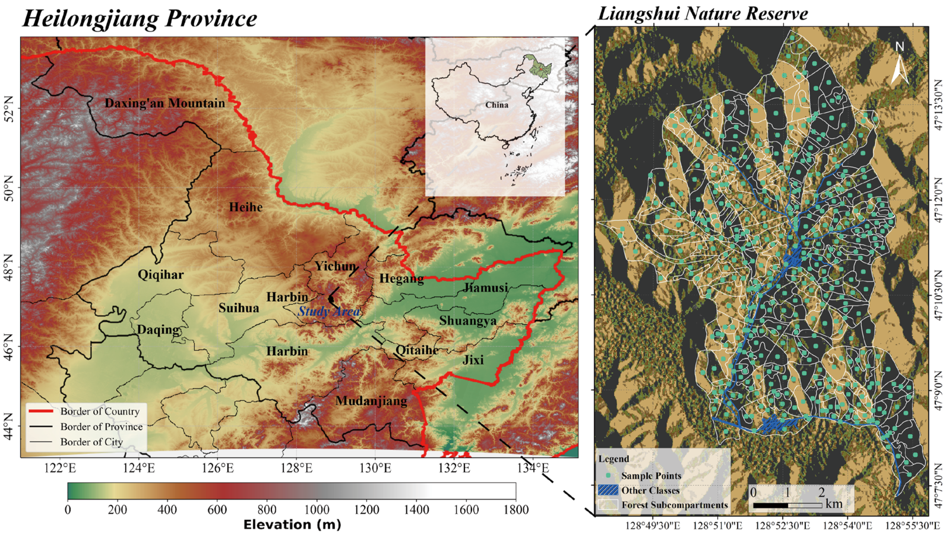
2.1. Study Areas

The total area of the reserve is 12,133 ha (Figure 1), and it is geographically located at the eastern edge of the Eurasian continent, with temperate continental monsoon climate characteristics [15]. Within the territory of the reserve, the mountains are surrounded by gullies and ravines, forming a more complex mountainous terrain. The average altitude of the whole area is approximately 400 m, and the relative height is between 80 and 300 m. To facilitate forest management and forestry surveys, the forest management department divided the reserve into 444 forest subcompartments according to stand composition and topography (steep slopes, flat land and pit land) of the study area, which made the stand composition and topographic distribution in each forest subcompartments basically the same, and we randomly selected one sample point in each forest subcompartment as the sample point for subsequent research. Because the zoning principle of subcompartments in this study area is basically the same small class with homogeneous forest types, the carbon stock information of each sample point represents the average carbon stock level of the subcompartment.

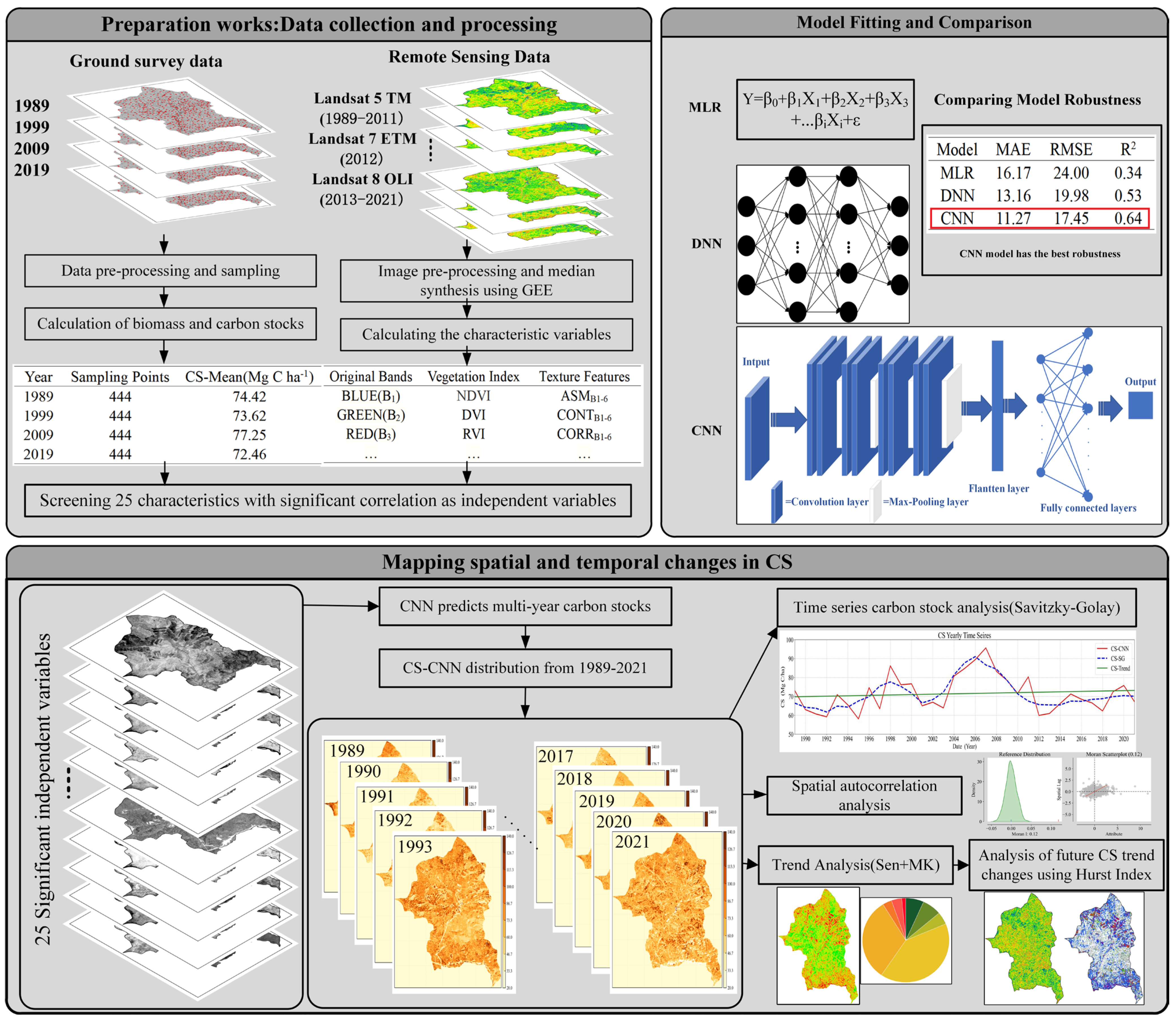
2.2. Data Acquisition and Treatment

2.2.1. Ground Survey Data

We collected and compiled data from the forest resource planning and design surveys conducted in 1989, 1999, 2009, and 2019, which consisted of comprehensive census data of protected areas within forest subcompartments. The data included tree height (m), diameter at breast height (cm), number of forest trees (n ha−1) and storage volume (m3 ha−1) from 444 forest subcompartments. To obtain the forest biomass of local native tree species more precisely, the biomass per hectare (Mg ha−1) of different forest types was calculated according to the anisotropic growth equations [30] proposed by Dong (Table 1). These growth equations have been extensively experimented and validated, and have high accuracy in the calculation of forest biomass. Based on Yu’s study on the carbon content of forests in Xiaoxinganling, a carbon conversion factor of 0.4412 was applied [31]. Forest biomass and the carbon conversion factor were used to derive forest carbon stocks (Mg C ha−1) for 444 forest subcompartments for 4 years. Due to the excessive number of pixels in the study area, we randomly selected one sample point on each forest subcompartment, which means there are 444 × 4 = 1776 sample points as the target variable. The formula for calculating the forest standing wood carbon stock (CS) is:
C S = Y S + Y B + Y F + Y R × ρ
YS, YB, YF and YR are the biomasses of the stems, branches, foliage and roots of trees, respectively, and ρ (0.4412) is the carbon stock conversion factor.
Table 1. Equations used for estimating the biomass of the different forest stands from the Xiaoxinganling Mountains following Dong 2015 [30]. In these equations, H is the average tree height (m), D is the average diameter at breast height (cm), N is the stand density (n/ha) and V is the storage volume (m3/ha).
Forest TypesBiomass Function
Birch forestYS = (H/(−0.7161 + 1.7316H))V
YB = (H/(71.1504 + 2.3594H))V
YF = (D/(52.1765 + 31.5260D))V
YR = (D/(−7.7814 + 5.2684D))V
Korean pine forestYS = (N/(369.6842 + 1.5593N))V
YB = 0.1807D0.1196H−0.1086V
YF = 0.2835D−0.2246H−0.2737V
YR = H/(−7.4947 + 5.4H))V)
Larch forestYS = 0.2638D0.6084H−0.3052V
YB = 0.0893D0.5372H−0.5798V
YF = (D/(−0.320.565 + 69.0763D))V
YR = (D/(44.2954 + 1.182D))V
Populus forestYS = 0.2472D0.134H−0.0461V
YB = (D/(70.9902 + 8.7291D))V
YF = (D/(−71.0595 + 22.4834D))V
YR = (D/(−7.72 + 0.1178D))V
Pinus sylvestris forestYS = 0.3063D0.2638H0.0044V
YB = 0.0809D0.3271H−0.282V
YF = (D/(−71.0595 + 22.4834D))V
YR = (D/(−25.67 + 7.3893D))V
Mixed broad-leaved forestYS = 0.5193D0.1529H−0.0981V
YB = (D/(79.2051 + 1.2886D))V
YF = (D/(−84.3635 + 42.2363D))V
YR = (H/(−6.079 + 5.4717H))V
Mixed coniferous broad-leaved forestYS = (D/(−1.3193 + 2.0249D))V
YB = (D/(58.0685 + 5.6768D))V
YF = (D/(−507.269 + 78.1762D))V
YR = (H/(−2.1908 + 5.6433H))V
Mixed coniferous forestYS = (D/(0.6756 + 2.1D))V
YB = 0.0631D0.3538H−0.2781V
YF = (D/(−156.921 + 43.4676D))V
YR = (D/(14.289 + 4.883D))V

2.2.2. Remote Sensing Data

Image data were acquired and processed in the GEE platform [32], and the goal was to collect continuous image data from 1989 to 2021; therefore, we choose data from the Landsat 5 TM (1989–2011), Landsat 7 ETM (2012) and Landsat 8 OLI (2013–2021) surface reflection sensor series images (LANDSAT/LT05/C01/T1_SR, LANDSAT/LE07/C01/T1_SR and LANDSAT/LC08/C01/T1_SR), which have a resolution of 30 m and adequate continuity [33]. The Landsat SR dataset has undergone radiation correction and atmospheric correction. We preprocessed the dataset with cloud removal and fusion processing [12]. The image data time range of 1 June to 31 October each year was chosen to match the ground survey data time and to eliminate the effect of seasonal differences on the data processing results. Finally, time series data with clear pixels were obtained by taking the median value.
The obtained time series images were used to calculate the features needed for the experiment (Table 2), including 6 raw bands (blue, green, red, NIR, SWIR1, SWIR2), 11 vegetation indices, and 18 texture features corresponding to the 6 raw bands, for a total of 125 features. Since different features have different magnitudes and units of magnitude, and as different satellite data may produce certain differences that can affect the results of data analysis, we normalized all features to eliminate the effect of magnitude among indicators [34]. Then, we used four years of ground survey data (1989, 1999, 2009 and 2019) as the target variables and chose the stepwise regression method to reduce the dimensionality of the feature variables. Next, we introduced each of the 125 feature variables into the regression equation, conducted significance tests and filtered 25 significant features (GREEN, NIR, SWIR1, ARVI, LST, MNDWI, MSAVI, NDBSI, RVI, SAVI, WDVI, DISSB1, PROMB1, VARB1, CONTB2, VARB2, DISSB3, INERB3, PROMB3, SVARB3, VARB3, DVARB4, SAVGB4, DISSB5, DISSB6).

3. Methodology

To develop a highly accurate and highly mobile regional scale model for predicting standing forest carbon stocks, we extracted spatial, temporal and spectral information from multitemporal multispectral data [32]. The independent variables were obtained by calculating vegetation indices and texture features, and the significant variables were screened by stepwise regression. In the prediction models, we first selected a multiple linear regression model (MLR) [47], a deep neural network model (DNN) [48] and a convolutional neural network model (CNN) [49] to determine the best model for predicting the standing forest carbon stock. The best predictive model was used to forecast the carbon stocks from 1989 to 2021 pixel by pixel, and specific distribution maps were drawn. A trend analysis was performed on the prediction results to determine the future direction of the standing wood carbon stock from forests. The specific process is shown in Figure 2.

3.1. Models

3.1.1. Multiple Linear Regression (MLR)

First, we selected a multiple linear regression model with parameter visualization for the study, with 25 characteristic variables identified as independent variables and forest carbon stock as the dependent variable. The number of sample points for 4 years was 1776, and 70% of the sample points (n = 1243) were randomly selected for the modeling of carbon stock estimation, while the remaining 30% of the sample data (n = 533) were used for accuracy verification. The mathematical model was:
Y = β 0 + β 1 X 1 + β 2 X 2 + β 3 X 3 + β 4 X 4 + + β ρ X ρ + ε
where Y is the forest carbon stock. X1,2,3ρ are the independent variables, where ρ indicates the identity (number) of the variable. βρ is the corresponding regression coefficient of each variable, and ε is the model residual.

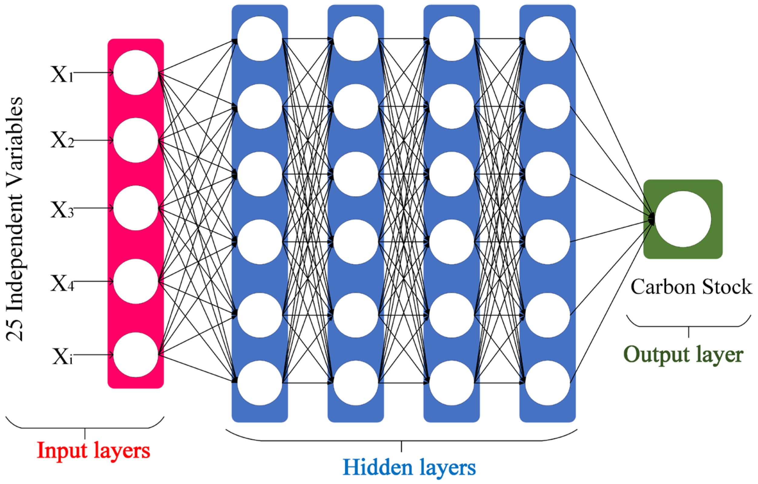
3.1.2. Deep Neural Networks (DNN)

A deep neural network was used to simulate the distribution of forest carbon stocks in the Liangshui Nature Reserve for 4 years. DNN is a powerful feed-forward machine learning mechanism that provides information about linear and nonlinear associations between a set of independent and dependent variables [50]. DNN is an artificial neural network with multiple layer structures, including input layers, multiple hidden layers and output layers. The hidden layers and built-in hyperparameters of DNN make them superior to other statistical models and classical machine learning models [51]. There is a connective structure between nodes in adjacent layers of the model, but there are no connections between nodes in the same layer or across layers. Different nodes are connected to each other in the form of fully connected layers with a combination of activation functions to build a multilayer complex neural network model. The model structure is shown in Figure 3.
DNN have been widely used in remote sensing in recent years [52]. DNN are trained using forward and backward propagation (BP) algorithms, which continuously update each weight (w) and bias (b) in the network. The backward propagation algorithm, which is the core of the DNN, essentially back-propagates the error between the predicted output value and the true value and continuously modifies the magnitude of w and b in each connection layer of the network model so that the error value is continuously reduced until it meets the accuracy requirement [53]. After the value of the loss function declines to the required threshold through the training of a large amount of data, the value of the parameter at this point is taken as the model parameter, and the regression prediction is performed accordingly. The weight and bias of the BP algorithm are calculated as follows:
w * = w α J w , b w
b * = b α J w , b b
where w* and w are the weights after and before the update, respectively; b* and b are the biases after and before the update, respectively; α is the artificially set learning rate; and J(w, b) is the loss function of the model. The optimal parameters w* and b* are obtained through continuous gradient descent iterations.

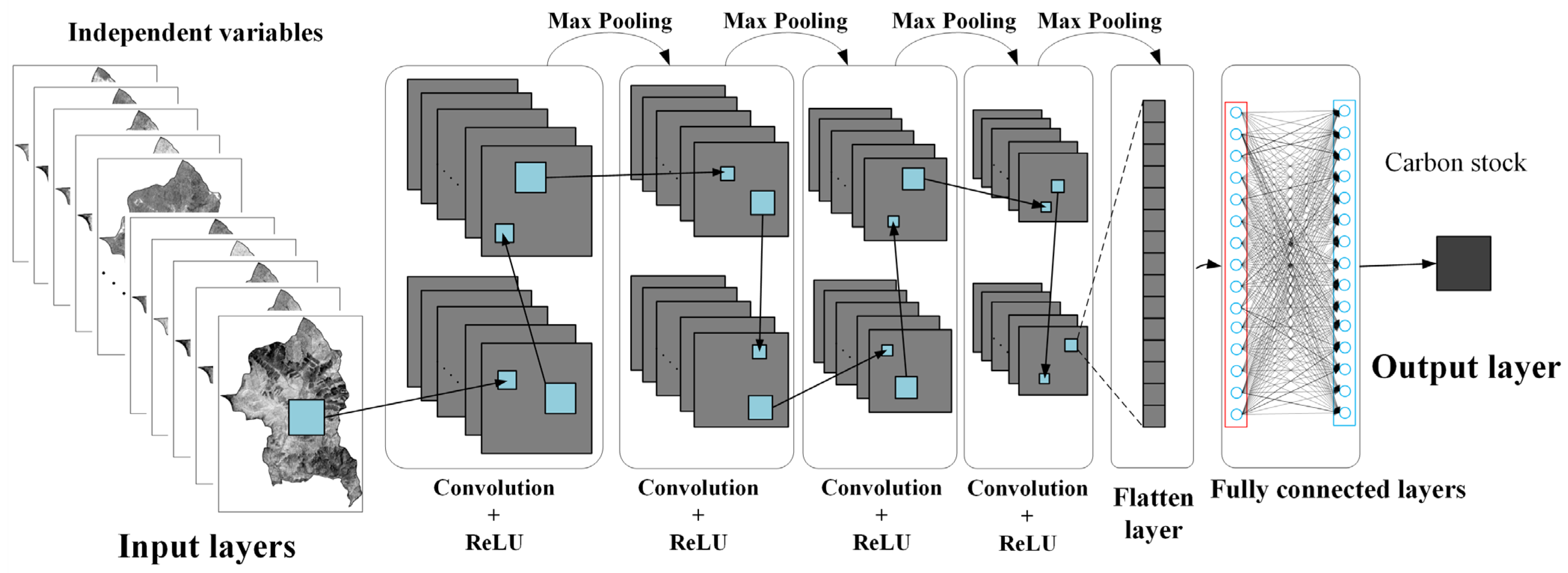
3.1.3. Convolutional Neural Network (CNN)

A convolutional neural network is a multilayer supervised, learning, fully connected or non-fully connected neural network structure, and the model structure is shown in Figure 4. The structural model of the convolutional neural network includes an input layer, a convolutional layer, a fully connected layer and an output layer [54]. The convolutional layer is a unique structure of the convolutional neural network that contains a set of kernels, or parameters that are learned throughout the training of a pooling layer that contains the data. The input signal and filter are convolved in the convolutional layer, and the implicit features of the input signal are iteratively extracted as the input of the next layer until the mapping relationship in the convolutional neural network converges to the predefined input–output mapping relationship or reaches the termination condition [55]. The number of convolutional layers in the network model is set to 8, and the size of the convolutional kernel is set to 1 × 3. Meanwhile, the ReLU [56] function is chosen as the activation function to avoid gradient disappearance due to the increase in the number of layers and the decline in the learning ability [57]. A max pooling layer is added after every two convolutional layers for downsampling, and only the information with larger weights in the feature mapping is retained to reduce the computational effort [58]. Finally, the information is aggregated to the fully connected layer for information regularization. A total of 25 remote sensing features were input as independent variables, 70% of the sample points were extracted as the training set (n = 1243) and the remaining 30% of the sample data were used as the test set (n = 533) for accuracy verification.

3.2. Evaluation Indicators

3.2.1. Model Evaluation Indicators

In this study, the fitting effectiveness of the MLR, DNN and CNN models was evaluated using three metrics. These metrics include mean absolute error (MAE), root mean square error (RMSE) and coefficient of determination (R2), where smaller MAE and RMSE values and larger R2 values indicate a more accurate fit of the models. The formulas of these evaluation indicators are shown below.
M A E = 1 n i = 1 n y i y i ^
R M S E = i = 1 n ( y i y i ^ ) n
R 2 = 1 i = 1 n ( y i y i ^ ) 2 i = 1 n ( y i y i ¯ ) 2
where n is the number of samples, y i is the actual observed carbon stock content of sample i, y i ^ is the predicted carbon stock content of sample i and y i ¯ is the actual observed mean value of carbon stock.

3.2.2. Spatial Autocorrelation Analysis

Exploratory spatial data analysis can be used to determine whether there is a correlation between the spatial distribution of standing forest carbon stocks and their neighboring regions and to describe the magnitude of the correlation. The main indicator for calculating spatial autocorrelation is Global Moran’s I [59]. Global Moran’s I is the most commonly used statistic in global correlation analysis and is mainly used to describe the average degree of correlation between a spatial unit and its surrounding area. The formula is [60]:
Globalmoran s   I = N i j w i j x i μ x j μ ( i j w i j ) i x i μ 2
where xi and xj are the carbon stock values at i and j, μ is the mean carbon stock value, wij is the spatial weight value between i and j and N is the total number of pixels. The value of Global Moran’s I varies between -1 and 1. When the value of Global Moran’s I is close to −1, it indicates that the negative spatial carbon stock autocorrelation is more significant, while when the value of Global Moran’s I is close to 1, it indicates that the carbon stock clustering effect is more significant. A Global Moran’s I value of 0 indicates no spatial autocorrelation.

3.2.3. Sen’s Slope Estimator

A simple nonparametric procedure developed by Sen (Sen, 1968; Hirsch et al., 1982) was used to estimate possible linear trends in the time series. The formula for calculating Sen’s slope is (10):
β = median X j X i j i     j > i
where β is the slope and the other term of the function represents the median value, where Xj and Xi are the data values at time j and i, respectively.

3.2.4. Mann–Kendall Statistical Test

The Mann–Kendall statistical test (MK) is a nonparametric statistical test that can be applied to the trend analysis of variables that are not normally distributed and are not subject to outlier images. The MK time series test formula is:
S = i = 1 n 1 j = i + 1 n f X j X i         j > i
f X j X i = + 1       i f X j X i > 0 0             i f X j X i = 0 1       i f X j X i < 0
V a r S = 1 18 n n 1 2 n + 5 p = 1 q t p ( t p 1 ) 2 t p + 5
where Xj and Xi are the data values at time j and i (j > i), respectively, n is the length of the time series, p is the number of repetitions, q is the number of unique numbers and tp is the number of repeats for each repetition. The formula for calculating the standard normal variable ZMK is:
Z M K = S 1 V a r S           i f     S > 0             0                 i f     S = 0 S + 1 V a r S       i f     S < 0
when |Z| ≤ Z1−α/2, the original hypothesis is accepted, and the trend is not significant; if |Z| > Z1−α/2, the original hypothesis is rejected, i.e., the trend is considered significant. If the significance level α = 0.05, then the critical value Z1−α/2 = ±1.96. When the absolute value of Z is greater than 1.96 and 2.58, the trend passes the significance test with 95% and 99% confidence levels, respectively [25]

3.2.5. Hurst exponent

The Hurst index is a key method for describing time series information [28] and it is widely used in meteorology and hydrology. The R/S method is based on the following principle: for a time series Xt (n) (n = 1, 2...), the mean series and the cumulative deviation are calculated as:
y τ = 1 τ n 1 τ X t n , τ = 1 , 2 ,  
f n , τ = n = 1 τ X t n y τ , 1 n τ
From this, the polar deviation and standard deviation are calculated:
R ( τ ) = max 1 t τ f ( n , τ ) min 1 t τ f n , τ , τ = 1 , 2 ,  
S ( τ ) = 1 τ n 1 τ X t n y τ 2 0.5 , τ = 1 , 2 ,
R ( τ ) / S ( τ ) = c τ H
where τ is the number of segments that split the time series into segments, n is the length of the time series, Xt(n) is the time series of length n, y τ is the mean of the time series, f n , τ is the cumulative deviation of the time series, c is a constant and H is the Hurst exponent, 0 < H < 1. Taking the logarithm of the left and right sides of the above equation yields
l o g ( R ( τ ) S ( τ ) ) = 1 H   l o g   τ + H   l o g   c
The Hurst exponent is denoted by H, and its value ranges from 0 to 1. When 0 < H < 0.5, it indicates that the future carbon stock trend is antiphased to the past trend, referred to as anti-sustainability change, and the closer the H value is to 0, the stronger the anti-sustainability. When 0.5 < H < 1, it indicates that the future carbon stock trend is the same as the past trend, which indicates continuous change in the same direction, and the closer the H value is to 1, the stronger the continuous change. When the value of H is 0.5, it indicates that the carbon stock time series is in an independent state and it constitutes a random series; thus, the future trend and the past trend are not correlated.

4. Results

4.1. Descriptive Statistics

The mean carbon stock value for four years (1989, 1999, 2009, 2019) of field survey data (total 1776 sample points) was 74.44 Mg C ha−1 with a standard deviation of 32.37 Mg C ha−1. The specific annual carbon stock statistics are shown in Table 3.

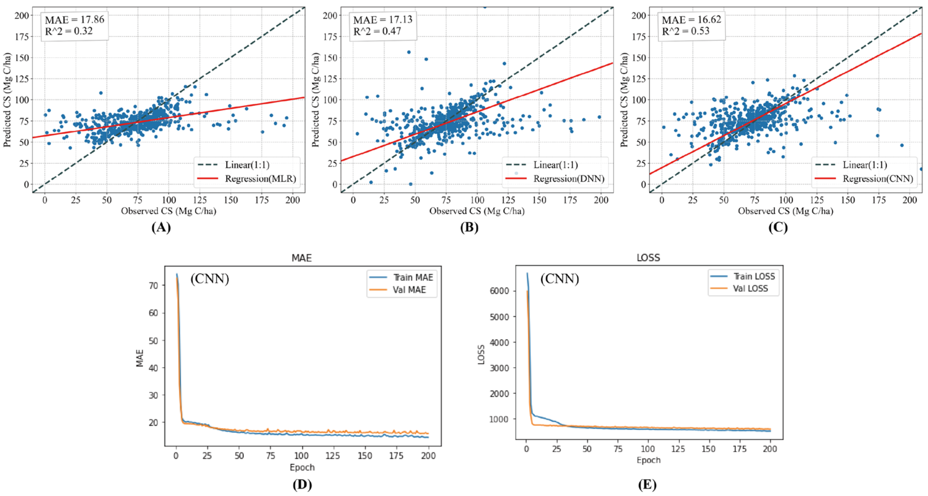
4.2. Evaluation of Models

In order to compare the fitting effect of different models, the ratio of training and validation data was chosen as 7:3 (1243:553), and ten combinations were randomly selected for control experiments to finally take the average value to evaluate the models. The evaluation results of the validation data of each model (MLR, DNN, CNN) are shown in Table 4. The traditional MLR model fit worse than the other models, while the DNN model fit better. The CNN model has the best fit robustness with carbon storage; the mean MAE is 16.62 Mg C ha−1 and the mean R2 is 0.53. Figure 5 shows the correlation between the observed and predicted carbon stocks of the different models, and the MAE decline curve, as well as the loss curve during the training of the CNN model, indicating that the model is not over-fitted. It can be seen that the CNN has a greater advantage in fitting carbon stocks.

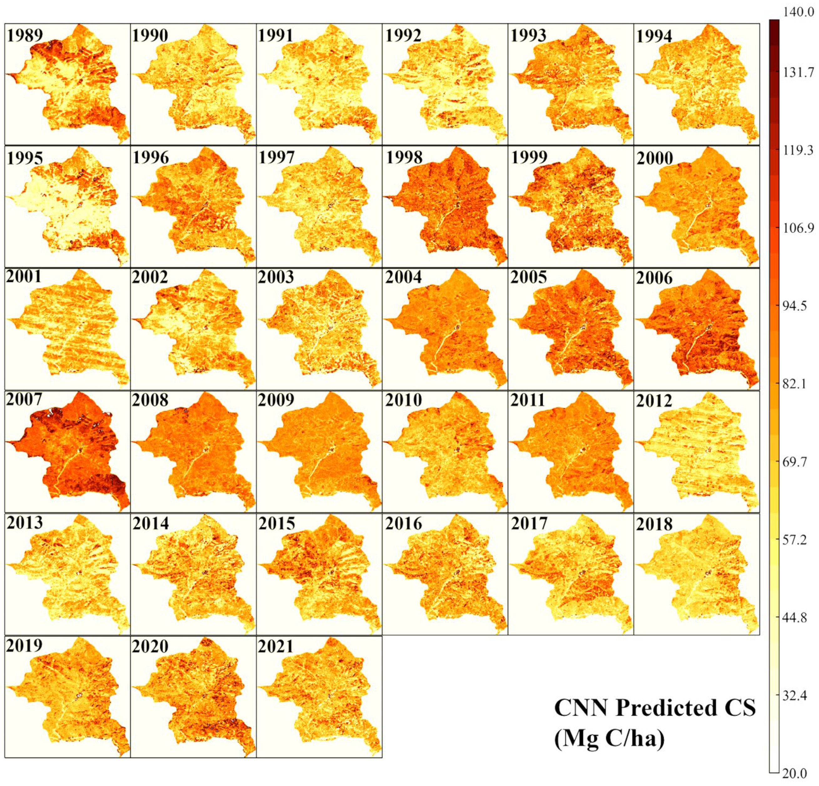
4.3. Optimal Model for Prediction

To obtain a more intuitive picture of the spatial and temporal variations in forest carbon stocks from 1989 to 2021, we used the CNN model, which had the highest robustness, to make predictions. All pixel values of the 25 significant variables for each year were substituted into the model to estimate the carbon stock distribution for the whole region in each year, and the results of the specific distribution are shown in Figure 6.
Meanwhile, we smoothed the mean carbon stock fold line (CS-CNN) of the time series using Savitzky–Golay filters [61] to better study the trend of carbon stock changes in the long time series (Figure 7). From the smoothed curve (CS-SG), we observed that the carbon stock tended to be stable from 1989 to 1995 (60–70 Mg C ha−1). However, it rose slightly to the peak from 1995 to 2001 (75–80 Mg C ha−1) and then began to decline. From 2001 onward, the carbon stock started to rise significantly with time and reached a peak in 2007 (90–95 Mg C ha−1). From 2007 to 2012, there was a significant downward trend in carbon stocks. From 2012 to 2021, there was a weak upward trend in carbon stocks (60–70 Mg C ha−1). We applied a trend fit (CS-Trend) to reflect the overall change in carbon stock in the time series, which showed that the overall change in carbon stock in the time series had increased.

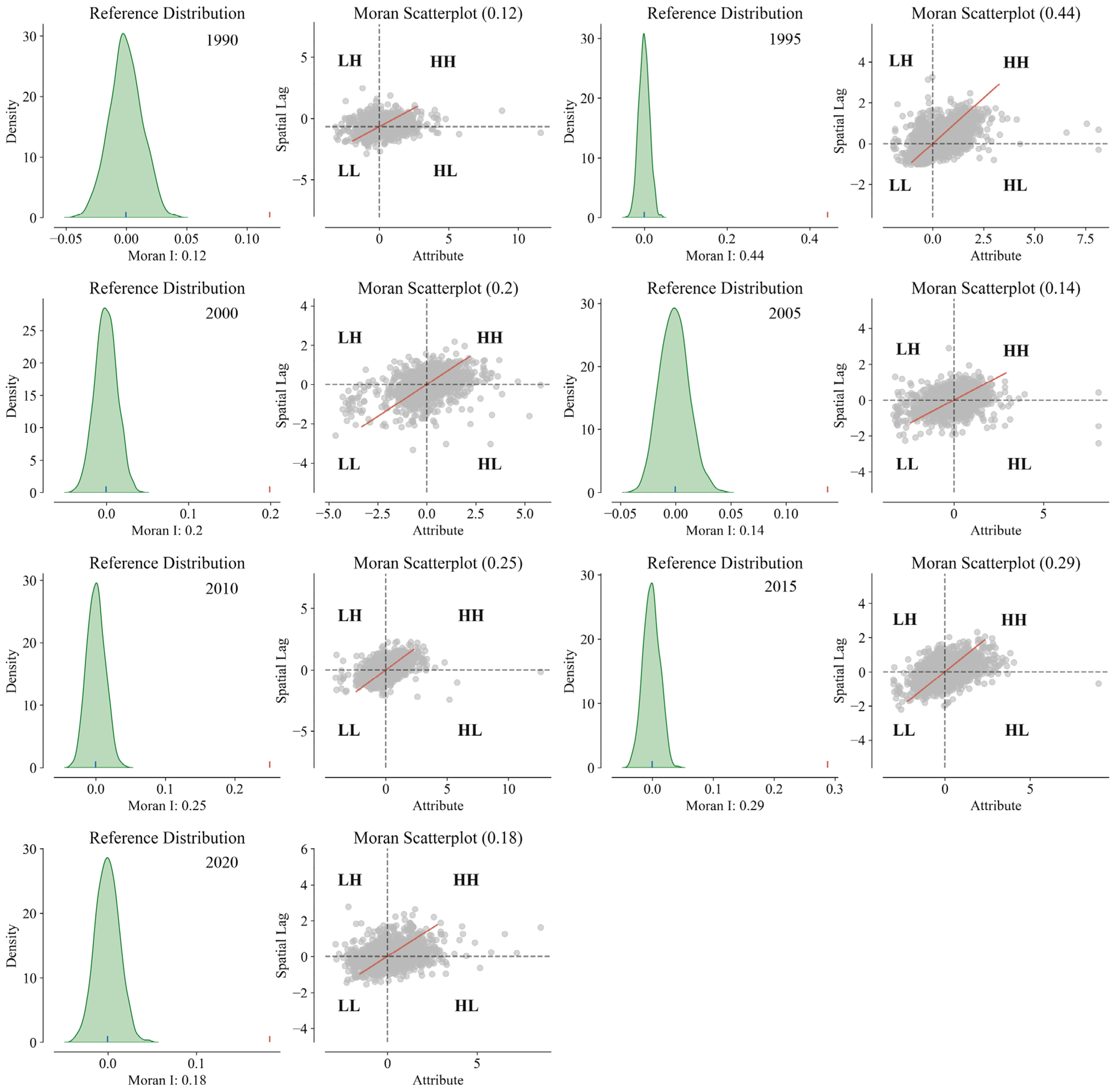
4.4. Spatial Autocorrelation Analysis of Carbon Stocks

To investigate whether there are other conditions for the spatial clustering phenomenon in the distribution of standing forest carbon stock in the study area, Moran’s I was introduced for analysis. From the predicted CS-CNN results, 2000 pixels (30 m × 30 m) were randomly extracted for spatial autocorrelation analysis. Because the change in forest carbon stock is a slow process, we selected CNN prediction results every 5 years (1990, 1995, 2000, 2005, 2010, 2015 and 2020) to study the autocorrelation analysis of forest carbon stock, which can avoid the chance error caused by the analysis of carbon stock in a single year. The Global Moran’s I of CS-CNN in 1990, 1995, 2000, 2005, 2010, 2015 and 2020 were 0.12, 0.44, 0.20, 0.14, 0.25, 0.29 and 0.18, respectively (Figure 8), all of which passed the test at the 1% significance level, and the results indicated that the spatial autocorrelation of carbon stock was significant at the 99% confidence level. The Moran scatterplot is divided into four quadrants, which indicate four local spatial correlations. Points in quadrant 1 are high-value regions and are surrounded by high-value regions; points in quadrant 2 are low-value regions and are surrounded by high-value regions; the point in quadrant 3 is a low-value region and is surrounded by low-value regions; the points in quadrant 4 are high-value regions and are surrounded by low-value regions. The Moran’s I of carbon stock in the study area is generally greater than 0, which shows a positive spatial correlation and indicates that carbon stock has different degrees of clustering effects.

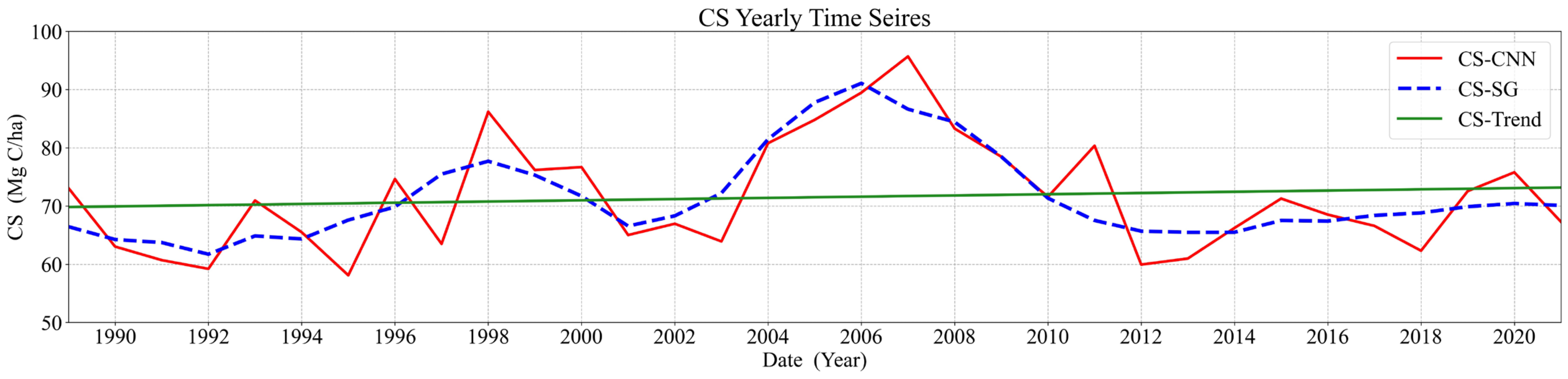
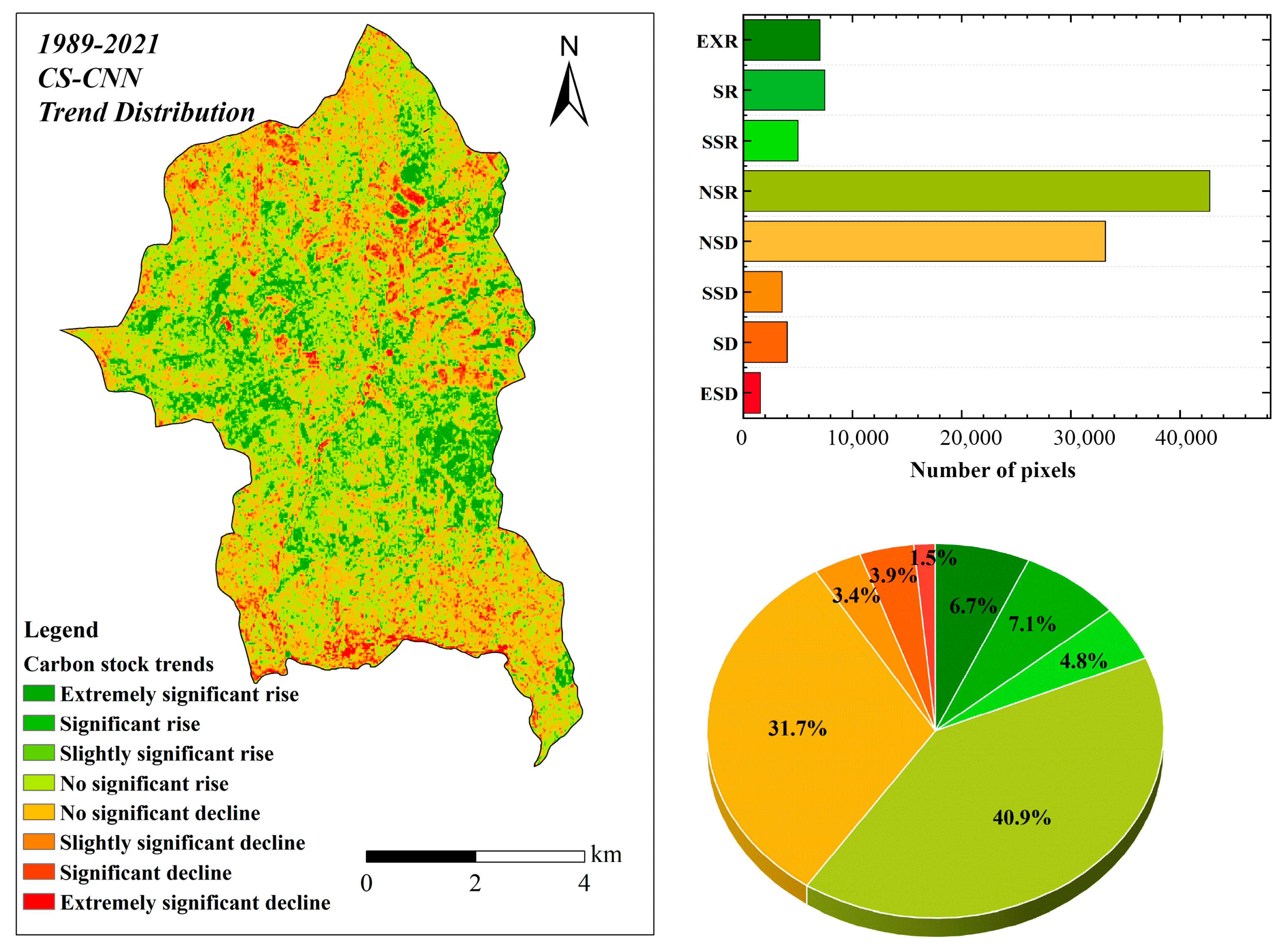
4.5. Trends in the Spatial Transformation of Carbon Stocks

Sen’s slope and the MK test were used to detect the spatial variation trends of the carbon stock, and the results were classified into eight categories: extremely significant rise, significant rise, slightly significant rise, no significant rise, extremely significant decline, significant decline, slightly significant decline and no significant decline. The specific distribution and percentages of the change trends are shown in Figure 9 and summarized as follows: 40.9% of the carbon stock showed no significant rise, mainly concentrated in the central part of the study area; 31.7% of the carbon stock showed no significant decreasing trends, mainly concentrated in the south and north of the study area; 18.6% showed extremely significant increasing, significant increasing and slightly significant increasing trends, concentrated in the north, west and east of the study area; 8.8% showed extremely significant decreasing, significant decreasing and slightly significant decreasing trends, mainly observed in the south and north-central regions of the study area. The total increasing trend accounted for 59.5% of all carbon stock, and the total decreasing trend accounted for 40.5%, indicating that the carbon stock in the study area has shown an overall increasing trend over the past 33 years, but some areas have exhibited a decreasing trend.

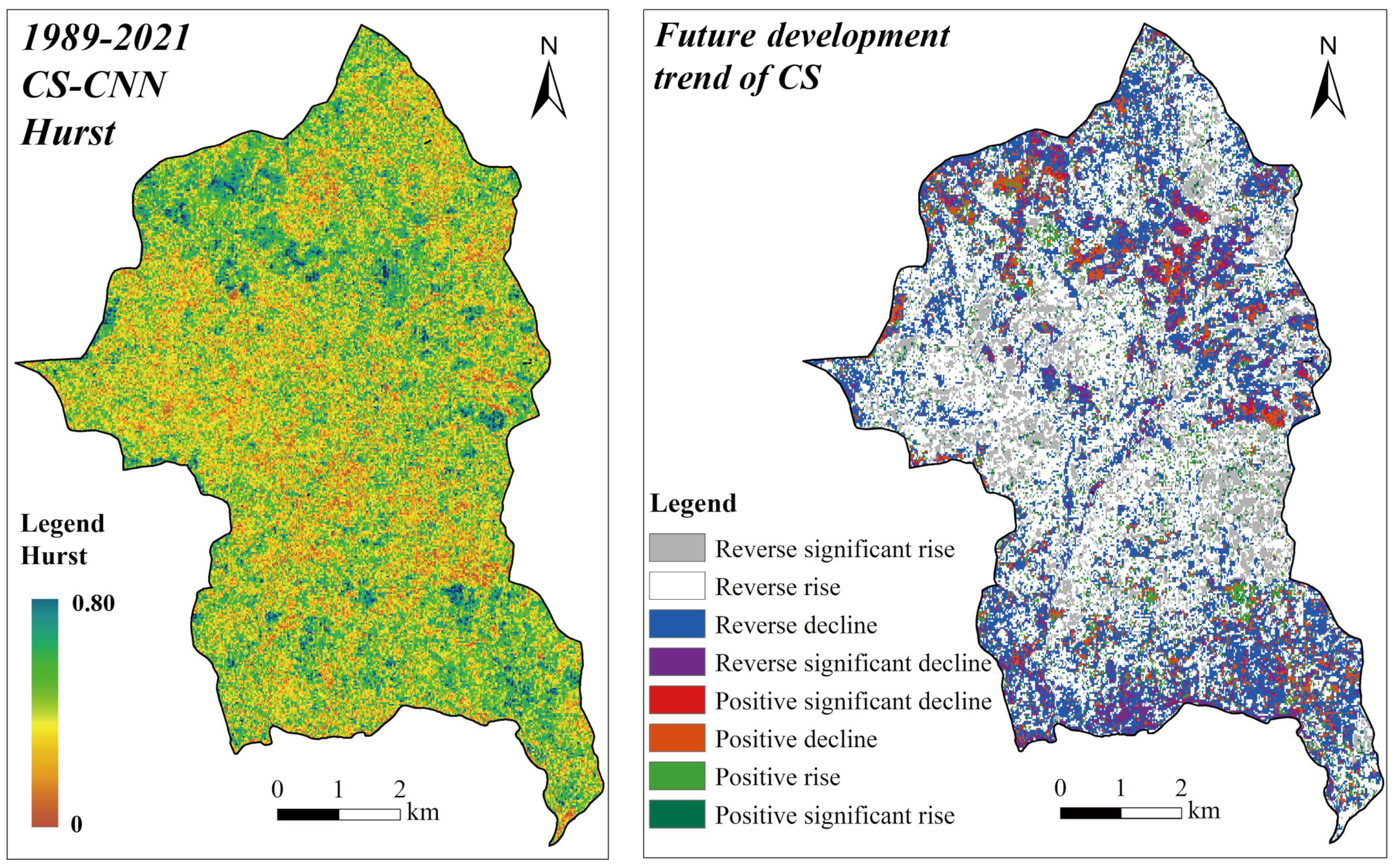
4.6. Future Trends in Forest Carbon Stocks

To better explore the future trends of carbon stocks in the study area, the Hurst exponent was calculated for the CNN prediction results from 1989 to 2021. This was then combined with the Sen and MK tests to determine the relationship between future evolution and past trends in the changes to vegetation cover in Heilongjiang Province (Figure 10). The Hurst exponent ranged from 0 to 0.80, with a mean value of 0.41, indicating that in the carbon stock study area, the overall change was characterized by reverse persistence since the Hurst exponent range between 0 and 0.5 is set as reverse persistence, and the exponent range between 0.5 and 1 is set as same direction persistence. However, Hurst exponents closer to 0.5 indicate weaker correlations between future changes and past trends for either reverse persistence or continuous change. The spatial carbon stock trends (significant increase, increase, significant decrease, decrease) were superimposed over the sustainability exponent H of these two types of change, and eight development trends were derived, including four types of benign development directions and four types of malignant development directions. Thus, this work demonstrated the change characteristics and future development trends of standing forest carbon stock in the study area.
The different future trends of forest carbon stocks as a percentage are shown in Table 5. The future development trend of the study area as a whole is likely to develop in a benign direction (60% of the future upward trend), and 6% of the regions are continuously rising (1% and 5% of the region show positive significant upward and positive upward trends, respectively). These few regions are distributed in the northwestern and southern parts of the study area. In the study area, 54% of the regions (the largest share of the trend) declined in the past but are on an upward trend now and are likely to remain so in the future. Of these regions, 13% show an anti-significant upward trend and 41% show anti-upward trends. These locations are mainly distributed in the central and western parts of the study region. The regions with a continuous decline accounted for 7% of the study area (positive significant decline and positive declining trend accounted for 1% and 6%, respectively), and were mainly distributed in the central and northwestern parts of the study region. The regions that showed a past rising trend but future declining trend accounted for 33% of the area (reverse significant decline and reverse declining trend accounted for 4% and 29%, respectively), and were concentrated in the north and south parts of the study region.

5. Discussion

Forest carbon stock is a component of the Earth’s carbon pool and an important indicator of ecosystem stability [62]. As a typical representative of the natural boreal secondary forest, the changes observed in the standing forest wood carbon stock in the study area reveal, to a certain extent, the variability of standing forest wood carbon stock in the whole Xiaoxinganling region. Therefore, understanding and predicting the spatial and temporal distribution of standing forest wood carbon stocks is essential for optimizing forest resource management and improving the carbon sequestration potential in this region, as well as mitigating adverse effects of climate change and related impacts.
In this study, a robust CNN model was trained using publicly available and easily accessible Landsat series satellite imagery and existing ground data. Then, the trained model was used to predict the carbon stock distribution from 1989 to 2021. Initially, we tried the MLR model with visible model parameters [63], but the carbon stock of forest stands and the related remote sensing factors did not have a completely linear relationship, and the performance of all indicators was average. Then, we tried deep learning algorithms that could better fit the nonlinear relationship and found that the CNN was the most suitable algorithm for carbon stock prediction, with high portability and better performance for high-dimensional input variables [64]. Because the carbon stock at a location is influenced by environmental conditions and surrounding locations, steep slopes can also affect the distribution of carbon stock [65]. CNN introduces spectral information and texture features, which can reflect the feature of the ground, into the model as independent variables, and also solves the problem of spatial heterogeneity to some extent. However, the CNN also has some limitations, such as underestimating the maximum or minimum carbon stock content due to the limited training set, which is also a drawback of global prediction. In subsequent research, local regression combined with deep learning can be used to make more accurate predictions of carbon stock content.
To observe the dynamic changes in continuous carbon stock time series, we choose the image datasets from the Landsat series of satellites [66], which have the longest operation and are continuously maintained. However, there are still some gaps between the remotely sensed data and the observations made directly in the field due to atmospheric attenuation, the low signal-to-noise ratio of the sensor itself, annual revisits and low resolution [67]. In particular, as the scale of the study area is extended from local to regional, the degradation of image quality will lead to greater errors in the analysis. In addition, defects in the remote sensing data itself can interfere with the experiment. In this study, remote sensing images from some years (2001, 2012) showed slight streaking due to the failure of the on-board scan line corrector of the Landsat satellite. The appearance of streaks in the original bands led to the same situation in the remote sensing factors extracted from them, which led to similar streaks in the CS-CNN predicted forest carbon stock mapping (Figure 6). The stripes makes the mapping look less than perfect, but the mean values of forest carbon stock projections are in the normal range and have little effect on the trend analysis (Figure 7). The other years of images do not have this problem, and the satellite data from 1989, 1999, 2009 and 2019 used to train the model are also normal, which means that the robustness of the model itself is not affected in any way. Subsequent observations and studies can include higher-resolution satellite hyperspectral images to predict or verify the changes in carbon stock patterns and multisource remote sensing data can be combined to achieve better results [68].
The results of this study show that the overall trend of forest carbon stocks in the study area is increasing. Especially between 1989 and 2007, the increasing trend was clear. Under the reasonable management of the protected area, the growth of forest stands reached the mature phase, and the stumpage carbon stock was close to the peak. Afterwards, most of the stands entered the overmature forest stage, the resistance of trees weakened and the carbon stock began to decline due to natural disasters before finally stabilizing. As the resistance of the overmature forest weakens, rapid climate change and the influence of human factors led to a decreasing trend in forest carbon stocks. Ultimately, forest carbon stock stabilized due to the self-regulation ability of the forest ecosystem.
The study found that forest carbon stock does not continually increase or decrease by following a single trend but increases or decreases periodically, which is consistent with natural relationships and reveals the feasibility and practicality of the study to a certain extent. However, we need to conduct more in-depth research to quantitatively explore the drivers of forest carbon stock changes, which includes anthropogenic factors and climate change. These considerations will help to more accurately predict forest carbon stock trends, which will in turn facilitate more precise forest carbon stock distribution mapping.

6. Conclusions

Based on the GEE platform and Landsat TM/ETM/OLI remote sensing data, we studied the long-term spatial and temporal variations in the carbon stocks of forest stands using remote sensing and deep learning methods and explored the development trend of carbon stocks in the study area in depth. The MLR model (RMSE = 24.00, R2 = 0.34) had a general week fitting effect. Therefore, we chose a deep learning algorithm to predict the carbon stocks in forest stands, and we found that this model (RMSE = 17.45, R2 = 0.64) had the best fit. The CNN with the best robustness was used to make pixel-by-pixel predictions of the carbon stock. It was found that the carbon stock was mostly stable from 1989 to 1995; after 1995, the carbon stock started to rise significantly and then began to decline and stabilize after reaching its peak in 2007. There was a weak upward carbon stock trend between 2012 and 2021. Then, we analyzed the trend of the carbon stock of forest stumpage in recent years by combining Sen and MK statistical tests. The total upward trend was 59.5%, and the total downward trend was 40.5%. Generally, the forest stumpage carbon stock in the study area has developed positively in recent years. Combined with the Hurst index, we analyzed the future development trend of the standing wood carbon stocks of the forests in the study area and found that the overall development trend for 60% of the study area is likely to be benign in the future. Subsequently, we will use more source data and more comprehensive methods to further study the characteristics of the changes in the entire northern ecosystem.

Author Contributions

Conceptualization, X.Z.; methodology, X.Z.; software, X.Z.; validation, X.Z.; formal analysis, X.Z.; investigation, Y.S.; resources, F.W.; writing—original draft preparation, X.Z.; writing—review and editing, Y.M.; visualization, X.Z.; supervision, X.Z.; data curation, Y.M.; project administration, W.J.; funding acquisition, W.J. All authors have read and agreed to the published version of the manuscript.

Funding

This research was funded by China National Key Research and Development Program (grant no. 2022YFD2201003-02) and the Special Fund Project for Basic Research in Central Universities (2572019CP08).

Informed Consent Statement

Informed consent was obtained from all subjects involved in the study.

Data Availability Statement

The data is confidential and cannot be disclosed.

Acknowledgments

All authors thank the Liangshui Nature Reserve for providing data and experimental support.

Conflicts of Interest

The authors declare that there are no conflicts of interest regarding the publication of this article.

References

  1. Zaninovich, S.C.; Gatti, M.G. Carbon Stock Densities of Semi-Deciduous Atlantic Forest and Pine Plantations in Argentina. Sci. Total Environ. 2020, 747, 141085. [Google Scholar] [CrossRef] [PubMed]
  2. Dalmonech, D.; Marano, G.; Amthor, J.S.; Cescatti, A.; Lindner, M.; Trotta, C.; Collalti, A. Feasibility of Enhancing Carbon Sequestration and Stock Capacity in Temperate and Boreal European Forests via Changes to Management Regimes. Agric. For. Meteorol. 2022, 327, 109203. [Google Scholar] [CrossRef]
  3. Dulamsuren, C. Organic Carbon Stock Losses by Disturbance: Comparing Broadleaved Pioneer and Late-Successional Conifer Forests in Mongolia’s Boreal Forest. For. Ecol. Manag. 2021, 499, 119636. [Google Scholar] [CrossRef]
  4. Romanov, A.A.; Tamarovskaya, A.N.; Gloor, E.; Brienen, R.; Gusev, B.A.; Leonenko, E.V.; Vasiliev, A.S.; Krikunov, E.E. Reassessment of Carbon Emissions from Fires and a New Estimate of Net Carbon Uptake in Russian Forests in 2001–2021. Sci. Total Environ. 2022, 846, 157322. [Google Scholar] [CrossRef]
  5. Xu, C.; Wang, B.; Chen, J. Forest Carbon Sink in China: Linked Drivers and Long Short-Term Memory Network-Based Prediction. J. Clean. Prod. 2022, 359, 132085. [Google Scholar] [CrossRef]
  6. Fremout, T.; Cobián-De Vinatea, J.; Thomas, E.; Huaman-Zambrano, W.; Salazar-Villegas, M.; Limache-de la Fuente, D.; Bernardino, P.N.; Atkinson, R.; Csaplovics, E.; Muys, B. Site-Specific Scaling of Remote Sensing-Based Estimates of Woody Cover and Aboveground Biomass for Mapping Long-Term Tropical Dry Forest Degradation Status. Remote Sens. Environ. 2022, 276, 113040. [Google Scholar] [CrossRef]
  7. Ding, Y.; He, X.; Zhou, Z.; Hu, J.; Cai, H.; Wang, X.; Li, L.; Xu, J.; Shi, H. Response of Vegetation to Drought and Yield Monitoring Based on NDVI and SIF. CATENA 2022, 219, 106328. [Google Scholar] [CrossRef]
  8. Qiu, R.; Li, X.; Han, G.; Xiao, J.; Ma, X.; Gong, W. Monitoring Drought Impacts on Crop Productivity of the U.S. Midwest with Solar-Induced Fluorescence: GOSIF Outperforms GOME-2 SIF and MODIS NDVI, EVI, and NIRv. Agric. For. Meteorol. 2022, 323, 109038. [Google Scholar] [CrossRef]
  9. Lemoine-Rodríguez, R.; Inostroza, L.; Zepp, H. Does Urban Climate Follow Urban Form? Analysing Intraurban LST Trajectories versus Urban Form Trends in 3 Cities with Different Background Climates. Sci. Total Environ. 2022, 830, 154570. [Google Scholar] [CrossRef]
  10. Li, J.; Song, C.; Cao, L.; Zhu, F.; Meng, X.; Wu, J. Impacts of Landscape Structure on Surface Urban Heat Islands: A Case Study of Shanghai, China. Remote Sens. Environ. 2011, 115, 3249–3263. [Google Scholar] [CrossRef]
  11. Zheng, Z.; Wu, Z.; Chen, Y.; Guo, C.; Marinello, F. Instability of Remote Sensing Based Ecological Index (RSEI) and Its Improvement for Time Series Analysis. Sci. Total Environ. 2022, 814, 152595. [Google Scholar] [CrossRef]
  12. Wang, Q.; Song, K.; Xiao, X.; Jacinthe, P.-A.; Wen, Z.; Zhao, F.; Tao, H.; Li, S.; Shang, Y.; Wang, Y.; et al. Mapping Water Clarity in North American Lakes and Reservoirs Using Landsat Images on the GEE Platform with the RGRB Model. ISPRS J. Photogramm. Remote Sens. 2022, 194, 39–57. [Google Scholar] [CrossRef]
  13. Gorelick, N.; Hancher, M.; Dixon, M.; Ilyushchenko, S.; Thau, D.; Moore, R. Google Earth Engine: Planetary-Scale Geospatial Analysis for Everyone. Remote Sens. Environ. 2017, 202, 18–27. [Google Scholar] [CrossRef]
  14. Parastatidis, D.; Mitraka, Z.; Chrysoulakis, N.; Abrams, M. Online Global Land Surface Temperature Estimation from Landsat. Remote Sens. 2017, 9, 1208. [Google Scholar] [CrossRef] [Green Version]
  15. Zhang, X.; Sun, Y.; Jia, W.; Wang, F.; Guo, H.; Ao, Z. Research on the Temporal and Spatial Distributions of Standing Wood Carbon Storage Based on Remote Sensing Images and Local Models. Forests 2022, 13, 346. [Google Scholar] [CrossRef]
  16. Zhen, Z.; Li, F.; Liu, Z.; Liu, C.; Zhao, Y.; Ma, Z.; Zhang, L. Geographically Local Modeling of Occurrence, Count, and Volume of Downwood in Northeast China. Appl. Geogr. 2013, 37, 114–126. [Google Scholar] [CrossRef]
  17. Tian, D.; Jiang, L.; Shahzad, M.K.; He, P.; Wang, J.; Yan, Y. Climate-Sensitive Tree Height-Diameter Models for Mixed Forests in Northeastern China. Agric. For. Meteorol. 2022, 326, 109182. [Google Scholar] [CrossRef]
  18. Yuan, Q.; Shen, H.; Li, T.; Li, Z.; Li, S.; Jiang, Y.; Xu, H.; Tan, W.; Yang, Q.; Wang, J.; et al. Deep Learning in Environmental Remote Sensing: Achievements and Challenges. Remote Sens. Environ. 2020, 241, 111716. [Google Scholar] [CrossRef]
  19. Ma, L.; Liu, Y.; Zhang, X.; Ye, Y.; Yin, G.; Johnson, B.A. Deep Learning in Remote Sensing Applications: A Meta-Analysis and Review. ISPRS J. Photogramm. Remote Sens. 2019, 152, 166–177. [Google Scholar] [CrossRef]
  20. Chen, Y.; Lin, Z.; Zhao, X.; Wang, G.; Gu, Y. Deep Learning-Based Classification of Hyperspectral Data. IEEE J. Sel. Top. Appl. Earth Obs. Remote Sens. 2014, 7, 2094–2107. [Google Scholar] [CrossRef]
  21. Vetrivel, A.; Gerke, M.; Kerle, N.; Nex, F.; Vosselman, G. Disaster Damage Detection through Synergistic Use of Deep Learning and 3D Point Cloud Features Derived from Very High Resolution Oblique Aerial Images, and Multiple-Kernel-Learning. ISPRS J. Photogramm. Remote Sens. 2018, 140, 45–59. [Google Scholar] [CrossRef]
  22. Wang, Y.; Zhang, J.; Tong, S.; Guo, E. Monitoring the Trends of Aeolian Desertified Lands Based on Time-Series Remote Sensing Data in the Horqin Sandy Land, China. CATENA 2017, 157, 286–298. [Google Scholar] [CrossRef]
  23. Sen, P.K. Estimates of the Regression Coefficient Based on Kendall’s Tau. J. Am. Stat. Assoc. 1968, 63, 1379–1389. [Google Scholar] [CrossRef]
  24. Hirsch, R.M.; Slack, J.R.; Smith, R.A. Techniques of Trend Analysis for Monthly Water Quality Data. Water Resour. Res. 1982, 18, 107–121. [Google Scholar] [CrossRef] [Green Version]
  25. Partal, T.; Kahya, E. Trend Analysis in Turkish Precipitation Data. Hydrol. Process. 2006, 20, 2011–2026. [Google Scholar] [CrossRef]
  26. Tabari, H.; Somee, B.S.; Zadeh, M.R. Testing for Long-Term Trends in Climatic Variables in Iran. Atmos. Res. 2011, 100, 132–140. [Google Scholar] [CrossRef]
  27. Gocic, M.; Trajkovic, S. Analysis of Changes in Meteorological Variables Using Mann-Kendall and Sen’s Slope Estimator Statistical Tests in Serbia. Glob. Planet. Change 2013, 100, 172–182. [Google Scholar] [CrossRef]
  28. Hurst, H.E. Long-Term Storage Capacity of Reservoirs. Trans. Am. Soc. Civ. Eng. 1951, 116, 770–799. [Google Scholar] [CrossRef]
  29. Wang, X.; Li, T.; Ikhumhen, H.O.; Sá, R.M. Spatio-Temporal Variability and Persistence of PM2.5 Concentrations in China Using Trend Analysis Methods and Hurst Exponent. Atmos. Pollut. Res. 2022, 13, 101274. [Google Scholar] [CrossRef]
  30. Dong, L. Biomass Modeling of Major Tree Species and stAnd Types in the Northeast Forest Region. Ph.D. Thesis, Northeast Forestry University, Harbin, China, 2015. [Google Scholar]
  31. Yu, Y.; Fan, W.; Li, M. Carbon content of forests at different scales in the Northeast Forest Region. J. Appl. Ecol. 2012, 23, 341–346. [Google Scholar] [CrossRef]
  32. Zhou, B.; Okin, G.S.; Zhang, J. Leveraging Google Earth Engine (GEE) and Machine Learning Algorithms to Incorporate in Situ Measurement from Different Times for Rangelands Monitoring. Remote Sens. Environ. 2020, 236, 111521. [Google Scholar] [CrossRef]
  33. Wulder, M.A.; Roy, D.P.; Radeloff, V.C.; Loveland, T.R.; Anderson, M.C.; Johnson, D.M.; Healey, S.; Zhu, Z.; Scambos, T.A.; Pahlevan, N.; et al. Fifty Years of Landsat Science and Impacts. Remote Sens. Environ. 2022, 280, 113195. [Google Scholar] [CrossRef]
  34. Martins, V.S.; Roy, D.P.; Huang, H.; Boschetti, L.; Zhang, H.K.; Yan, L. Deep Learning High Resolution Burned Area Mapping by Transfer Learning from Landsat-8 to PlanetScope. Remote Sens. Environ. 2022, 280, 113203. [Google Scholar] [CrossRef]
  35. Tucker, C.J. Red and Photographic Infrared Linear Combinations for Monitoring Vegetation. Remote Sens. Environ. 1979, 8, 127–150. [Google Scholar] [CrossRef] [Green Version]
  36. Xue, J.; Su, B. Significant Remote Sensing Vegetation Indices: A Review of Developments and Applications. J. Sens. 2017, 2017, e1353691. [Google Scholar] [CrossRef] [Green Version]
  37. Baret, F.; Guyot, G. Potentials and Limits of Vegetation Indices for LAI and APAR Assessment. Remote Sens. Environ. 1991, 35, 161–173. [Google Scholar] [CrossRef]
  38. Tanre, D.; Holben, B.N.; Kaufman, Y.J. Atmospheric Correction Algorithm for NOAA-AVHRR Products: Theory and Application. IEEE Trans. Geosci. Remote Sens. 1992, 30, 231–248. [Google Scholar] [CrossRef]
  39. Huete, A.R. A Soil-Adjusted Vegetation Index (SAVI). Remote Sens. Environ. 1988, 25, 295–309. [Google Scholar] [CrossRef]
  40. Clevers, J.G.P.W. Application of the WDVI in Estimating LAI at the Generative Stage of Barley. ISPRS J. Photogramm. Remote Sens. 1991, 46, 37–47. [Google Scholar] [CrossRef]
  41. Qi, J.; Chehbouni, A.; Huete, A.R.; Kerr, Y.H.; Sorooshian, S. A Modified Soil Adjusted Vegetation Index. Remote Sens. Environ. 1994, 48, 119–126. [Google Scholar] [CrossRef]
  42. Xu, H. Modification of Normalised Difference Water Index (NDWI) to Enhance Open Water Features in Remotely Sensed Imagery. Int. J. Remote Sens. 2006, 27, 3025–3033. [Google Scholar] [CrossRef]
  43. Jimenez-Munoz, J.C.; Cristobal, J.; Sobrino, J.A.; Soria, G.; Ninyerola, M.; Pons, X. Revision of the Single-Channel Algorithm for Land Surface Temperature Retrieval From Landsat Thermal-Infrared Data. IEEE Trans. Geosci. Remote Sens. 2009, 47, 339–349. [Google Scholar] [CrossRef]
  44. Hu, X.; Xu, H. A New Remote Sensing Index for Assessing the Spatial Heterogeneity in Urban Ecological Quality: A Case from Fuzhou City, China. Ecol. Indic. 2018, 89, 11–21. [Google Scholar] [CrossRef]
  45. Baig, M.H.A.; Zhang, L.; Shuai, T.; Tong, Q. Derivation of a Tasselled Cap Transformation Based on Landsat 8 At-Satellite Reflectance. Remote Sens. Lett. 2014, 5, 423–431. [Google Scholar] [CrossRef]
  46. Haralick, R.M.; Shanmugam, K.; Dinstein, I. Textural Features for Image Classification. IEEE Trans. Syst. Man Cybern. 1973, SMC-3, 610–621. [Google Scholar] [CrossRef] [Green Version]
  47. Egbueri, J.C.; Igwe, O.; Omeka, M.E.; Agbasi, J.C. Development of MLR and Variedly Optimized ANN Models for Forecasting the Detachability and Liquefaction Potential Index of Erodible Soils. Geosystems Geoenvironment 2023, 2, 100104. [Google Scholar] [CrossRef]
  48. Schyns, P.G.; Snoek, L.; Daube, C. Degrees of Algorithmic Equivalence between the Brain and Its DNN Models. Trends Cogn. Sci. 2022, 26, 1090–1102. [Google Scholar] [CrossRef]
  49. Akbarimajd, A.; Hoertel, N.; Hussain, M.A.; Neshat, A.A.; Marhamati, M.; Bakhtoor, M.; Momeny, M. Learning-to-Augment Incorporated Noise-Robust Deep CNN for Detection of COVID-19 in Noisy X-Ray Images. J. Comput. Sci. 2022, 63, 101763. [Google Scholar] [CrossRef]
  50. Wang, Y.; Zhang, Z.; Feng, L.; Du, Q.; Runge, T. Combining Multi-Source Data and Machine Learning Approaches to Predict Winter Wheat Yield in the Conterminous United States. Remote Sens. 2020, 12, 1232. [Google Scholar] [CrossRef] [Green Version]
  51. El Bilali, A.; Lamane, H.; Taleb, A.; Nafii, A. A Framework Based on Multivariate Distribution-Based Virtual Sample Generation and DNN for Predicting Water Quality with Small Data. J. Clean. Prod. 2022, 368, 133227. [Google Scholar] [CrossRef]
  52. Osco, L.P.; Marcato Junior, J.; Marques Ramos, A.P.; de Castro Jorge, L.A.; Fatholahi, S.N.; de Andrade Silva, J.; Matsubara, E.T.; Pistori, H.; Gonçalves, W.N.; Li, J. A Review on Deep Learning in UAV Remote Sensing. Int. J. Appl. Earth Obs. Geoinf. 2021, 102, 102456. [Google Scholar] [CrossRef]
  53. Taghizadeh-Mehrjardi, R.; Schmidt, K.; Amirian-Chakan, A.; Rentschler, T.; Zeraatpisheh, M.; Sarmadian, F.; Valavi, R.; Davatgar, N.; Behrens, T.; Scholten, T. Improving the Spatial Prediction of Soil Organic Carbon Content in Two Contrasting Climatic Regions by Stacking Machine Learning Models and Rescanning Covariate Space. Remote Sens. 2020, 12, 1095. [Google Scholar] [CrossRef] [Green Version]
  54. Zhu, X.X.; Tuia, D.; Mou, L.; Xia, G.-S.; Zhang, L.; Xu, F.; Fraundorfer, F. Deep Learning in Remote Sensing: A Comprehensive Review and List of Resources. IEEE Geosci. Remote Sens. Mag. 2017, 5, 8–36. [Google Scholar] [CrossRef] [Green Version]
  55. Kattenborn, T.; Leitloff, J.; Schiefer, F.; Hinz, S. Review on Convolutional Neural Networks (CNN) in Vegetation Remote Sensing. ISPRS J. Photogramm. Remote Sens. 2021, 173, 24–49. [Google Scholar] [CrossRef]
  56. Krizhevsky, A.; Sutskever, I.; Hinton, G.E. ImageNet Classification with Deep Convolutional Neural Networks. Commun. ACM 2017, 60, 84–90. [Google Scholar] [CrossRef] [Green Version]
  57. Briechle, S.; Krzystek, P.; Vosselman, G. Silvi-Net—A Dual-CNN Approach for Combined Classification of Tree Species and Standing Dead Trees from Remote Sensing Data. Int. J. Appl. Earth Obs. Geoinf. 2021, 98, 102292. [Google Scholar] [CrossRef]
  58. Hamraz, H.; Jacobs, N.B.; Contreras, M.A.; Clark, C.H. Deep Learning for Conifer/Deciduous Classification of Airborne LiDAR 3D Point Clouds Representing Individual Trees. ISPRS J. Photogramm. Remote Sens. 2019, 158, 219–230. [Google Scholar] [CrossRef] [Green Version]
  59. Zhang, Y.; She, J.; Long, X.; Zhang, M. Spatio-Temporal Evolution and Driving Factors of Eco-Environmental Quality Based on RSEI in Chang-Zhu-Tan Metropolitan Circle, Central China. Ecol. Indic. 2022, 144, 109436. [Google Scholar] [CrossRef]
  60. Oden, N.L. Spatial Processes: Models & Applications. A. D. Cliff, J.K. Ord. Q. Rev. Biol. 1982, 57, 236–236. [Google Scholar] [CrossRef]
  61. Savitzky, A.; Golay, M.J.E. Smoothing and Differentiation of Data by Simplified Least Squares Procedures. Anal. Chem. 1964, 36, 1627–1639. [Google Scholar] [CrossRef]
  62. Franklin, J.F.; Spies, T.A.; Pelt, R.V.; Carey, A.B.; Thornburgh, D.A.; Berg, D.R.; Lindenmayer, D.B.; Harmon, M.E.; Keeton, W.S.; Shaw, D.C.; et al. Disturbances and Structural Development of Natural Forest Ecosystems with Silvicultural Implications, Using Douglas-Fir Forests as an Example. For. Ecol. Manag. 2002, 155, 399–423. [Google Scholar] [CrossRef]
  63. Xie, D.; Li, X.; Zhou, T.; Feng, Y. Estimating the Contribution of Environmental Variables to Water Quality in the Postrestoration Littoral Zones of Taihu Lake Using the APCS-MLR Model. Sci. Total Environ. 2022, 857, 159678. [Google Scholar] [CrossRef] [PubMed]
  64. Wadoux, A.M.J.-C. Using Deep Learning for Multivariate Mapping of Soil with Quantified Uncertainty. Geoderma 2019, 351, 59–70. [Google Scholar] [CrossRef] [Green Version]
  65. Yang, L.; Cai, Y.; Zhang, L.; Guo, M.; Li, A.; Zhou, C. A Deep Learning Method to Predict Soil Organic Carbon Content at a Regional Scale Using Satellite-Based Phenology Variables. Int. J. Appl. Earth Obs. Geoinf. 2021, 102, 102428. [Google Scholar] [CrossRef]
  66. Barta, K.A.; Hais, M.; Heurich, M. Characterizing Forest Disturbance and Recovery with Thermal Trajectories Derived from Landsat Time Series Data. Remote Sens. Environ. 2022, 282, 113274. [Google Scholar] [CrossRef]
  67. Xia, L.; Zhao, F.; Chen, J.; Yu, L.; Lu, M.; Yu, Q.; Liang, S.; Fan, L.; Sun, X.; Wu, S.; et al. A Full Resolution Deep Learning Network for Paddy Rice Mapping Using Landsat Data. ISPRS J. Photogramm. Remote Sens. 2022, 194, 91–107. [Google Scholar] [CrossRef]
  68. Chen, R.; Zhang, C.; Xu, B.; Zhu, Y.; Zhao, F.; Han, S.; Yang, G.; Yang, H. Predicting Individual Apple Tree Yield Using UAV Multi-Source Remote Sensing Data and Ensemble Learning. Comput. Electron. Agric. 2022, 201, 107275. [Google Scholar] [CrossRef]
Figure 1. Geographical location of the study area and forests subcompartments distribution in the Liangshui Nature Reserve.
Forests 14 00483 g001
Figure 2. Research flow chart: including data collection and pre−processing (calculation of forest carbon stocks, extraction and calculation of remote sensing factors and characteristics screening), model fitting and comparison (MLR, DNN and CNN), spatial and temporal distribution of carbon stocks, and trend analysis (time series carbon stock trend analysis, spatial autocorrelation analysis, future carbon stock development trend).
Forests 14 00483 g002
Figure 3. Scheme of a deep neural network framework, including input layers, multiple hidden layers and output layers.
Forests 14 00483 g003
Figure 4. Schematic structure of the convolutional neural network model, including an input layer, a convolutional layer, a fully connected layer and an output layer.
Forests 14 00483 g004
Figure 5. (A) is the fitting result from the MLR; (B) is the fitting result from the DNN; (C) is the fitting result from the CNN; (E) shows the decline curve of CNN model MAE; (D) shows the loss curve of the CNN model training and validation data.
Forests 14 00483 g005
Figure 6. Distribution of the CNN model’s pixel-by-pixel carbon stock (Mg C/ha) projection results for 1989–2021, and the carbon stock distribution range is 20–140 Mg C/ha.
Forests 14 00483 g006
Figure 7. Time series average CS distribution trend, CS-CNN is the prediction curve of CNN model, CS-SG is the curve after the Savitzky–Golay filter smoothing curve, and CS-Trend is the overall development trend of CS-CNN.
Forests 14 00483 g007
Figure 8. Global Moran’s I and Moran scatterplot of CS in 1990, 1995, 2000, 2005, 2010, 2015 and 2020. Quadrant 1 (HH) is a high-value area surrounded by other high-value areas. Quadrant 2 (LH) is a low-value area surrounded by high-value areas. Quadrant 3 (LL) is a low-value area surrounded by low-value areas. Quadrant 4 (HL) is a high-value area surrounded by low-value areas.
Forests 14 00483 g008
Figure 9. CS spatial variation trend map and the percentages of different trends.
Forests 14 00483 g009
Figure 10. Hurst distribution map and CS future trend map.
Forests 14 00483 g010
Table 2. Original bands, vegetation indices and texture features included in the analysis performed through the GEE platform. The corresponding calculation formula is provided for remote sensing factors when applicable.
Remote Sensing DataBands, Indices or ParametersDefinition or Calculation Formula
Original bandBLUE(B1)Water penetration, distinguishing soil vegetation
GREEN(B2)Distinguishing different vegetation
RED(B3)Observation of roads, bare soil, and vegetation types
NIR(B4)Estimating biomass and distinguishing wet soils
SWIR1(B5)Distinguishing the road, bare leaking soil
SWIR2(B6)Heat distribution mapping, rock identification
Vegetation IndexNormalized Difference Vegetation Index (NDVI) [35](NIR − RED)/(NIR + RED)
Difference Vegetation Index (DVI) [36]NIR − RED
Ratio Vegetation Index (RVI) [37]NIR/RED
Atmospheric Ratio Vegetation Index (ARVI) [38](NIR − (2 × RED − BLUE))/(NIR + (2 × RED − BLUE))
Soil-Adjusted Vegetation Index (SAVI) [39]((NIR − RED)/(NIR + RED + 0.5))(1 + 0.5)
Weighted Difference Vegetation Index (WDVI) [40]NIR − 0.5 × RED
Modified Soil-Adjusted Vegetation Index (MSAVI) [41](2NIR + 1 − ((2 × NIR + 1) − 8 × (NIR − RED))0.5)/2
Modified Normalized Difference Water Index (MNDWI) [42](NIR − GREEN)/(NIR + GREEN)
Land Surface Temperature (LST) [43]T/(1 + (λT/ρ)lnε);
λ is the central wavelength of thermal infrared band, ρ = 1.438 × 10⁻² m·k; ε is the surface specific emissivity
Normalized Difference Building and Soil Index (NDBSI) [44](SI + IBI)/2;
SI and IBI represent the soil index and building index, respectively
Wetness (WET) [45]β1BLUE + β2GREEN + β3RED + β4NIR + β5SWIR1 + β6SWIR2;
β1–6 are the different coefficients corresponding to different sensor types
Texture featuresAngular Second Moment (ASMB1–6)The texture metrics are calculated from the grayscale co-occurrence matrix around each pixel in each band. The grayscale co-occurrence matrix is a list of the frequency of occurrence of different combinations of pixel luminance values (grayscale) in an image. It calculates the number of times a pixel with value X is adjacent to a pixel with value Y in a specific direction and distance, and then derives statistics from this table [46].
Contrast (CONTB1–6)
Correlation (CORRB1–6)
Variance (VARB1–6)
Inverse Difference Moment (IDMB1–6)
Sum Average (SAVGB1–6)
Sum Variance (SVARB1–6)
Sum Entropy (SENTB1–6)
Entropy (ENTB1–6)
Difference variance (DVARB1–6)
Difference entropy (DENTB1–6)
Information Measure of Corr. 1 (IMCORR1B1–6)
Information Measure of Corr. 2 (IMCORR2B1–6)
Max Corr. Coefficient (MAXCORRB1–6)
Dissimilarity (DISSB1–6)
Inertia (INERB1–6)
Cluster Shade (SHADEB1–6)
Cluster prominence (PROMB1–6)
Table 3. Ground survey data statistics.
YearCS-Mean
(Mg C ha−1)
CS-Standard Deviation
(Mg C ha−1)
CS-Median
(Mg C ha−1)
198974.4238.3571.65
199973.6240.4167.29
200977.2524.4178.55
201972.4621.8770.57
Table 4. The MLR, DNN and CNN model result summary for validation data.
CombinationMLRDNNCNN
MAER2MAER2MAER2
117.580.3416.870.5116.320.54
218.160.2917.090.4816.870.52
318.010.3517.320.4216.340.54
417.960.3117.290.4517.110.49
517.600.3416.840.5116.380.53
617.870.3216.980.4916.900.51
718.210.2817.130.4716.230.57
817.540.3517.280.4616.270.56
917.710.3217.320.4116.970.50
1017.970.3117.190.4316.840.52
Mean17.860.3217.130.4616.620.53
Table 5. The percentage of different future change trends in CS.
Change DirectionsFuture TrendsPercentage
Continuous declinePositive significant decline0.01
Positive decline0.06
Rise in the past but declining trend in the futureReverse significant decline0.04
Reverse decline0.29
Decline in the past but rising trend in the futureReverse significant rise0.13
Reverse rise0.41
Continuous risePositive significant rise0.01
Positive rise0.05
Disclaimer/Publisher’s Note: The statements, opinions and data contained in all publications are solely those of the individual author(s) and contributor(s) and not of MDPI and/or the editor(s). MDPI and/or the editor(s) disclaim responsibility for any injury to people or property resulting from any ideas, methods, instructions or products referred to in the content.

