Comparative Analysis of Remote Sensing and Geo-Statistical Techniques to Quantify Forest Biomass

Abstract

Accurately characterizing carbon stock is vital for reporting carbon emissions from forest ecosystems. We studied the estimation of biomass using Sentinel-2 remote sensing data in moist temperate forests in the Galies region of Abbottabad Pakistan. Above-ground biomass (AGB), estimated from 60 field plots, was correlated with vegetation indices obtained from Sentinel-2 image-to-map AGB using regression models. Furthermore, additional explanatory variables were also associated with AGB in the geo-statistical technique, and kriging interpolation was used to predict AGB. The results illustrate that the atmospherically resistant vegetation index (ARVI) is the best index (R² = 0.67) for estimating AGB. In spectral reflectance, Band 1(Coastal Aerosol 443 nm) performs better than other bands. Multiple linear regression models calibrated with ARVI, NNIR and NDVI yielded better results (R² = 0.46) with the lowest RMSE (48.53) and MAE (38.42) and were therefore considered better for biomass estimation. On the other hand, in the geo-statistical technique, distance to settlements, ARVI and annual precipitation were significantly correlated with biomass compared to others. In the stepwise regression method, the forward selection resulted in a very significant value (less than 0.000) for ARVI. Therefore, it can be considered best for prediction and used to interpolate AGB through kriging. Compared to the geo-statistical technique, the remote sensing-based models performed relatively well. Regarding potential sites for REDD+ implementation, temporal analysis of Landsat images showed a decrease in forest area from 8896.23 ha in 1988 to 7692.03 ha in 2018. Therefore, this study concludes that the state-of-the-art open-source sensor, the Sentinel-2 data, has significant potential for forest biomass and carbon stock estimation and can be used for robust regional AGB estimation with acceptable accuracy and frequent availability.

1. Introduction

Forest ecosystems are among the largest terrestrial carbon reservoirs on Earth, as global forests hold the most extensive stock of terrestrial carbon stored in living trees. However, due to various anthropogenic activities (social pressure), when deforestation occurs or is degraded in terms of its structure and function (forest degradation), this leads to emissions of stored carbon into the atmosphere, thus contributing to environmental changes [1,2]. Reducing Emissions from Deforestation and Forest Degradation (REDD+) is an initiative to reduce deforestation and carbon emissions from forest ecosystems in developing countries. REDD+ also includes the conservation of forests, sustainable forest management and enhancing carbon stocks to facilitate developing countries in climate change mitigation [3,4]. The REDD+ activities can be validated and monitored through the Measuring, Reporting and Verification (MRV) system, the central part of the REDD+ mechanism, which ensures proper forest inventories and carbon estimation following national baselines or reference levels (RLs) [5,6,7]. The MRV system mainly focuses on the assessment of carbon stocks based on forest reference emission levels (FRELs), which develop an auditable, transparent, comparable, consistent, complete and verifiable national forest monitoring system (NFMS) as per UNFCCC requirements [2,8]. Reported data through MRV system must be accurate, comprehensive and comparable over spatio-temporal scales.

NFMS’s MRV system comprisesa two-stage procedure; in the first stage, FRELs of the developing country are technically assessed, followed by the second stage, in which the developing country submits reports about emission reductions compared to national FRELs [9] Subsequently, separate third-party REDD+ experts technically assess and verify the reports of the developing country for provision of finance, compensation and incentives based on carbon sequestration [10]. In order to ensure impartial carbon estimates with minimum uncertainty, pre-defined methods with thresholds for emissions, time, scale and area should be determined [11]. Pakistan’s MRV system operates through NFMS ((https://www.nfmspak.org/) (accessed on 19 January 2023)) through forest department, non-governmental organizations and local communities in order to implement all phases of REDD+ [12]. In Pakistan, significant work has been conducted on the MRV system for REDD+; standards were developed for NFI and a satellite monitoring system (called Satellite Land Monitoring (SLM)) throughout the country [13]. In this context, Pakistan’s NFMS has developed three pillars (SLMS and NFI integrated with GHG inventory) as per guidelines of UN-REDD. Pakistan’s SLMS of MRV system, extensively used Landsat images for LULC categories/classes through systematic grid points across the country based on the reference years starting from 1996 to 2016 with intervals of four years [14],as well as further work of the SLMS, is in progress under the Ministry of Climate Change of Pakistan ((https://www.redd-pakistan.org/) (accessed on 19 January 2023). Currently, like MRV systems of other developing countries [15], Pakistan’s SLMS has successfully assessed deforestation over recent decades using temporal satellite images; however, quantifiable information about forest degradation is still a challenging task at the national level [14]. Data about forest degradation (as a vital component of REDD+) have been collected and verified by territorial forest staff and community members and reported to NFMS [14]. Previously, many studies reported that the local MRV system of a particular region, in which local communities participated in carbon inventory under the supervision of forest staff [16,17,18,19], encourages forest dwellers to not only carry out REDD+ activities but also provide monitoring data for NFMS MRV [12,20,21]. In Pakistan, remote sensing (the SLMS) is considered as one of the best monitoring sources for the REDD+ MRV system [22] and open-source satellite imagery (such as Sentinel-2) may be utilized to monitor and estimate changes in the carbon stocks over a wide range of spatio-temporal scales.

In the context of FRELs, large-scale forest inventories are required at national, regional and local levels to estimate forest carbon stock and biomass over time. Forest biomass can be assessed using destructive or non- destructive sampling [23]. The destructive method involves harvesting all trees and measuring the biomass of different parts [24]. However, it is limited to small areas because it is expensive and harvesting all trees is impossible for large areas. Non-destructive sampling methods involve various forest attribute measurements and biomass assessment through different allometric equations [25]. Forest inventories provide the best biomass and carbon estimates of the sampled area if these inventories are detailed, accurate, controlled and intensive. However, traditional inventory techniques lack continuous spatial coverage, are time-consuming and require higher costs and labor.

Moreover, accessibility (to every part and parcel of land surface) and quantitative data regarding forest degradation are always a big challenge in forest biomes [7]. Therefore, the Intergovernmental Panel on Climate Change (IPCC) recommended three tiers to minimize such uncertainties; a higher tier means higher methodological complexity and improved accuracy [2]. Using remote sensing and geographic information systems (GISs), coupled with the national forest inventory (NFI), is usually acclaimed and can prove to be a robust method for carbon accounting [1,15]. Remote sensing technologies have minimized the problems and constraints associated with field data collection to a large extent. The use of remote sensing for forest biomass and carbon stock estimation can be implemented with acceptable accuracy [26]. The integrated approach of RS and NFI proves that accurate carbon stock estimation is vital for developing a baseline and reference levels for REDD+ implementation [15].

In the context of REDD+, RS technology has been used in both central themes of REDD+, such as forest degradation detection and its quantitative analysis [7,27], as well as for quantitative assessments of deforestation and its contributions as emissions [28]. Numerous sensors have been used to map, monitor and estimate forest biomass and carbon at various scales [15]. Landsat is one of the pioneers in the RS industry, which has a widely used sensor for various forestry applications, such as estimation of forest parameters [29]; forest trees’ age, height and biomass estimation [30]; vegetation cover change [31], forest height prediction [32]; forest types classification [33] above-ground biomass estimation [34] and forest monitoring through time series analysis [35]. REDD+ projects used Landsat for different purposes, such as mapping and monitoring deforestation and forest degradation [36,37] and referring to emissions levels [38]. This study used Sentinel-2 imagery for biomass estimation and mapping. Sentinel-2 is a state-of-the-art remote sensing product freely available for various vegetation applications. The high spatial, spectral and temporal resolution make the Sentinel-2 product most suitable for vegetation studies. The sentinel-2 product has 13 spectral bands in which about 9–10 bands can be used for different vegetation applications. These bands are Band 2 (Blue), Band 3 (Green), Band 4 (Red), Band 5, 6,7 (Red-edge bands), Band 8 and 8A (NIR), Band 11 and 12 (SWIR). The broadband indices are widely used indices for biomass mapping and have been extensively published by researchers using the Sentinel-2 product [39,40,41]. The presence of three red-edge bands in Sentinel-2 makes it suitable for various biophysical parameter computations.

Moreover, other techniques, such as non-parametric models, interpolation and geo-statistical techniques, such as kriging, are also frequently used for AGB prediction and mapping [42,43]. Geo-statistical methods have been employed to explore the AGB data’s spatial variation and design the most favorable sampling method for satellite images and in situ forest inventory [44]. The spatial distribution of forest attributes is not continued over the large mountainous landscape. However, essential tree attributes within stand type, such as diameter, height and volume, are controlled by different geospatially continued factors, including soil type, soil texture, nutrients, solar radiation, soil moisture and water-holding capacity [45]. It has been reported by previous studies that forest tree attributes measured during inventory, such as tree diameter, height, density, tree volume, AGB, etc., have spatial autocorrelation in a limited area within a particular stand type [46,47]. Still, such spatial autocorrelation becomes discontinued in the case of complex topography, anthropogenic pressures and commercial cutting areas [42]. Numerous studies reported integrating remote sensing methods with ordinary kriging and random forests for AGB estimation [44,48]. Specifically, such a combination is most suitable for the prediction of large areas with uneven topography and bioclimatic conditions [45,49]. Still, few studies published on AGB estimation, specifically in topographically complex forests in Pakistan, use geo-statistical methods combined with remote sensing techniques. In this context, this research uses Sentinel-2 RS data for biomass estimation and compares them with a geo-statistical technique (kriging interpolation). The main objectives of the present study are (1) to estimate above-ground biomass and carbon sequestration potential of forest area, (2) to explore the relationship between spectral bands and indices with biomass using simple, multiple and stepwise linear regression models and (3) to compare the linear regression models with global datasets to explore various potential sites for REDD+ implementation.

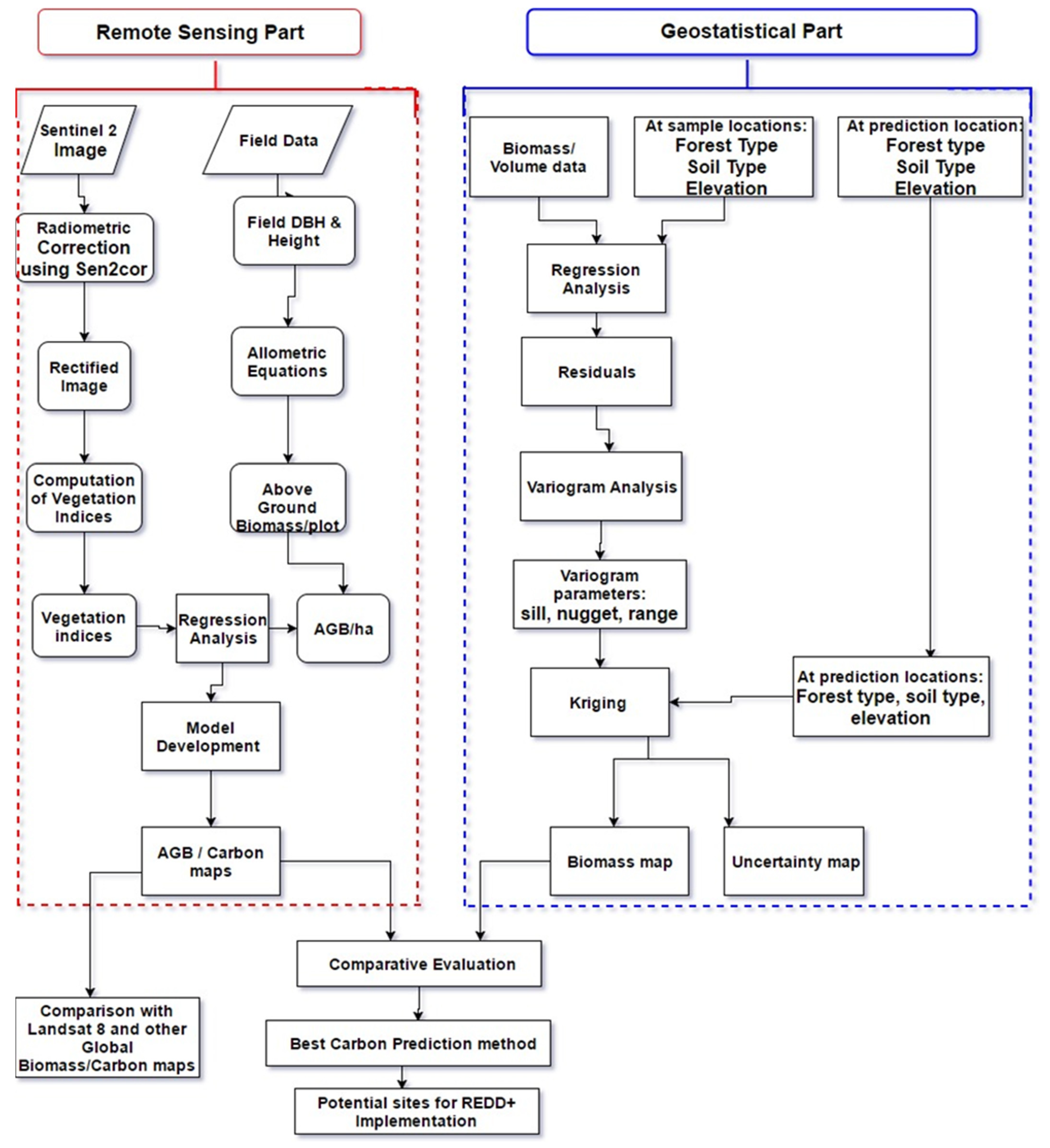
2. Materials and Methods

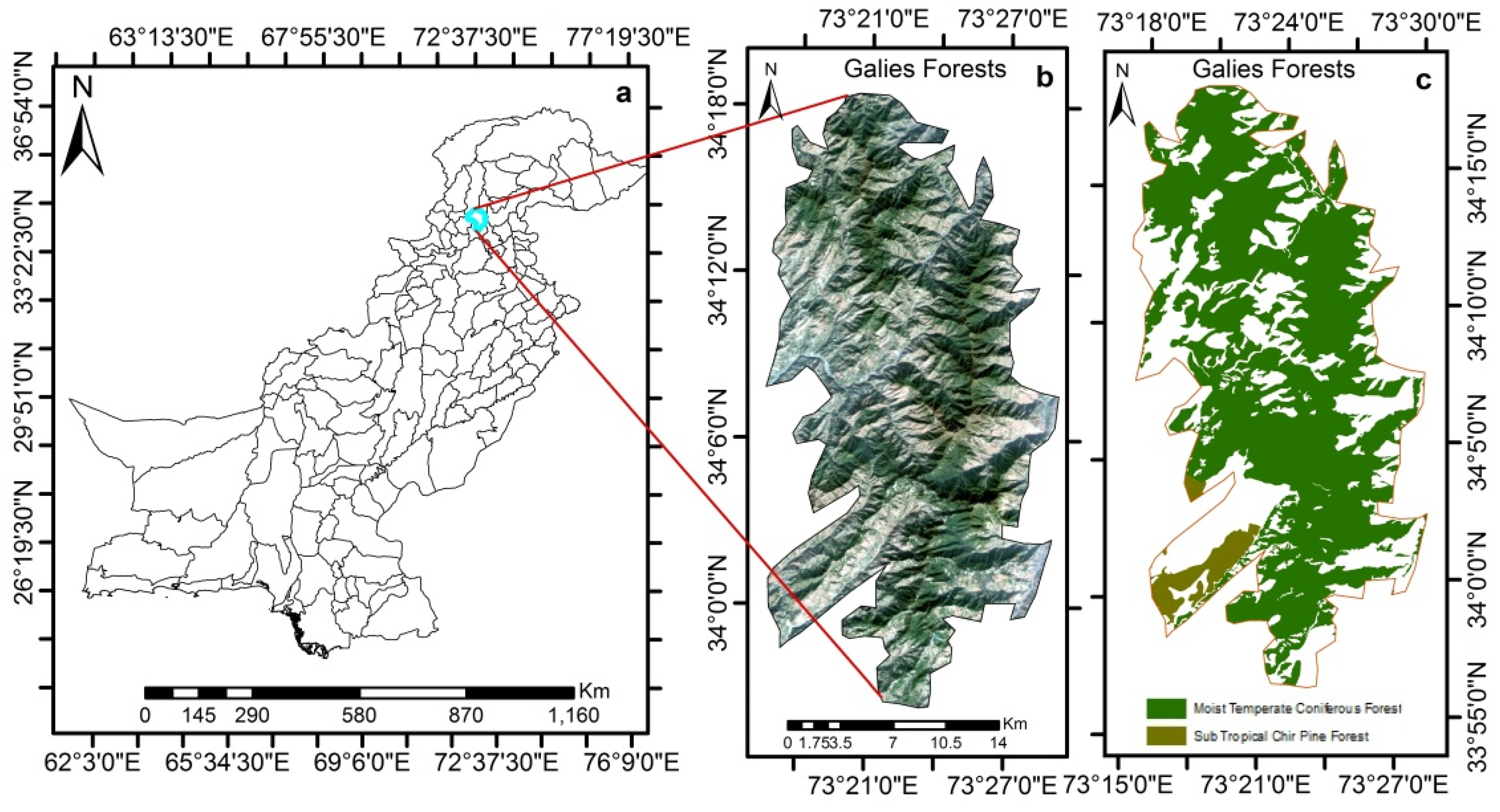
2.1. Study Area

The study area of the present research is the Galis forests located in the Abbottabad district of the Hazara forest division, Pakistan. The study area is located approximately between 33°55′ and 34°20′ north latitude and 73°20′ and 63°30′ east longitude. The Galis forests are on rugged, steep and precipitous slopes rising from 1067 to 2439 m. Galis forests’ climate represents both the dry sub-tropical and temperate zones. Sub-tropical arid climate lies on the western tract of Abbottabad, whereas the northern tract roughly falls in the cold temperate zone. January and February are the coldest months, whereas March and April are pleasant. May and June are hot and dry months. Monsoon rains tend to start in the middle of September.

The major forest types are (i) ub-tropical pine forests, (ii) low-level blue pine forests and (iii) Western mixed coniferous forests. Sub-tropical pine forests are located between the temperate and the dry sub-tropical vegetation. The altitudinal range of occurrence of Chir pine (Pinus roxburghii) varies from 920 to 1828 m in elevation. The principal broadleaved associate is oak (Quercus incana), with small amounts of other broadleaved species of Mallotusphillipinensis and Lyonia ovalifolia. Low-level blue pine forests extend over half of the study area and have better stocking than different coniferous forest types. The broadleaved associates are oak (Quercus dilitata and Quercus incana) and Prunus padus, mostly depressions and moist nullahs. Western mixed coniferous forests cover a minor portion of the total area of the forests, and their composition varies at different places. Still, the bulk of the growing stock consists of blue pine, deodar and silver fir.

2.2. Forest Inventory Part

This research used tier 2 methodology to estimate biomass and quantify the carbon sequestration potential in the study area. The tiered approach is based on the accuracy and complexity of inventory and resources required for these inventories [2]. A total of 60 plots were laid out to collect field data for AGB estimation in moist temperate forests, as illustrated in Figure 1 with the support of forest department. Data were collected from stratified random plots using field protocols as described in [23,50], keeping in view limiting factors such as time, resources, accessibility and steep slopes. As per the scope of the research, data were collected from 60 plots representing the AGB heterogeneity in the forest strata. Plot measurements were carefully performed, considering slope correction and ensuring horizontal distance. Errors in field measurements should be rectified before final data processing [51] because they affect the results and inventory accuracy [52]. The sampling plots’ size and shape were decided per UNFCCC (2015) guidelines. The shape of the plots was circular, having an area of 0.1 ha and 17.84 m radius. The plot measurements include species composition, forest type, geodetic coordinates, elevation, aspect, diameter at breast height (DBH), tree height and crown cover using diameter tape, Hagaalimter, Garmin eTrex 30× GPS, Sunntocampass, ranging rods and topographic maps. Geodetic coordinates and elevation were recorded using GPS receiver and subsequently the aspect was calculated based on coordinates using a digital elevation model. DBH of all trees (having ≥5 cm diameter) was measured at 4.5 feet or 1.3 m above the ground from the collar point of trees as per field measurement standard [50], while Haga Altimeter measured the height of the trees using trigonometric ratio of tree top and base with predefined distance. Sunnto Compass navigated directions from the plot to the plot, and a measuring tape was used for plot-to-plot and within-plot distance measurements [14,29]. Trees with defects, such as buttressed or forked trees, were also measured. Data were entered in the departmental field inventory forms taken from Pakistan Forest Institute (PFI), Peshawar. The data were transferred to Microsoft Excel sheets where biomass and carbon stocks were calculated. Biomass and carbon stocks were calculated by using allometric equations. The allometric equations are the regression equations between two or more forest attributes that can be used to estimate tree height, biomass or other growth attributes [53,54]. Thus, biomass can be estimated using field measurements such as diameter and height [55], as height represents tree primary growth and diameter represents secondary tree growth. The allometric equations used in this study to estimate biomass for inventoried species were taken from Pakistan Forest Institute, Peshawar (Supplementary Table S1). These allometric equations were specie- and site-specific and could only be used for the study area. Furthermore, AGB in kgs per plot was upscaled per hectare by multiplying the plot AGB by 10 because our plot size was one-tenth of a hectare. The AGB in tons was obtained by multiplying by 1000. Lastly, above-ground carbon stocks (AGCs) were determined by multiplying biomass in tons with a conversion factor of 0.47, as per explained in [40,56]. The conversion factor depicted that half of the dry biomass is carbon stocks for the given specie. The below-ground biomass (BGB) and below-ground carbon stocks (BGCs) were estimated by multiplying the AGB and AGC with a conversion factor of 0.26 [2,24,40]. The total carbon stocks were determined by adding AGC and BGC and then converted into CO₂ equivalent by multiplication of 3.66 with total carbon stocks. This conversion factor (3.66) is the ratio of molecular mass to atomic mass of carbon. Species wise biomass and carbon stocks have been estimated from the field inventory data and departmental data (for the year 2017) by using the literature’sbiomass expansion factor (BEF) and wood density. Likewise, species wise biomass and carbon stocks for the year 1984 have been estimated from the in situ inventory data of forest management plan. Moreover, temporal deforestation (1984 to 2017) has been estimated using two different datasets which include departmental stocked area (ha) and Landsat temporal images (Landsat-5 for 1984 and Landsat-8 for 2017). Subsequently, the carbon density and emission factors were calculated as described in the Technical Guidance for Emission Factors from deforestation ((https://www.un-redd.org/) (accessed on 17 July 2022)). Finally, carbon sequestration potential (CSP) was estimated from carbon carrying capacity (CCC) and estimated carbon density as described by [57].

2.3. Sentinel-2 Product Processing

Two Sentinel-2A products were downloaded from Copernicus Open-Access Hub ((https://scihub.copernicus.eu/dhus/#/home) (accessed on 27 September 2019)) for the study area. The Sentinel-2A products were ortho-rectified in UTM 43N Zone/WGS 84 projection and datum (Universal Transverse Mercator 43N Zone/World Geodetic System 1984). The processing and product levels of the acquired tile were Level-1C and S2MSI1C, respectively, and were obtained on 28 October 2018 for Galies Forest Abbottabad. S2A product was acquired for the date close to forest inventory time while keeping in view product quality. The acquired image has the least cloud cover in the study area (Supplementary Figure S1). Sentinel-2A products are composed of 100 by 100 km² tiles and provide top-of-the-atmosphere (TOA) reflectance measurements. Sentinel-2A was selected for this study since it has a high resolution compared to other open-source satellite products. Sentinel-2 provides a spatial resolution of 10 m in red, blue, green, near-infrared bands and 20 m spatial resolution in three additional red-edge bands, making it suitable for vegetation analyses. Sentinel-2 products were explored in ESA Sentinel Application Platform (SNAP) 5.0, the Sentinel-2 toolbox, downloaded from ((http://step.esa.int/main/download/) (accessed on 16 October 2019)). Sentinel-2 products (Level-1C) were preprocessed using the Sen2Cor plugin in SNAP 5.0 (It have been developed by Europian Space agency (ESA), https://step.esa.int/main/snap-5-0-released/ (accessed on 16 October 2019)). Sen2Cor is a third-party plugin in SNAP 5.0. which processed Level-1C products into Level-2A outputs using ESA’s algorithms [58]. Level 2A processing by Sen2Cor includes the conversion of top-of-the-atmosphere (ToA) ortho-rectified reflectance into atmospherically corrected outputs, i.e., bottom-of-the-atmosphere (BoA) reflectance [59]. The Sen2Cor processing was completed in multi-steps in an orderly manner; it first began with cloud detection and scene classification and further proceeded to aerosol optical thickness (AOT) and the water vapor (WV) content retrieval, ultimately resulting in Level-2A output [59]. After preprocessing, the Level-2A outputs were resampled to 10 m’ resolution for further analysis. Furthermore, shape files of study sites and inventory points were imported on the output Level-2A image. Subsets of the image were performed using the raster analysis tool in SNAP 5.0. The processed images were analyzed for various spectral indices using the “thematic land processing” option under “optical” tools in SNAP 5.0. SNAP 5.0 is user-friendly software that computed vegetation indices (VIs) with better quality for further analysis, i.e., biomass mapping, as depicted in Figure 2. The vegetation indices are mathematical transformations that can highlight vegetated areas in the images and can subsequently be easily used for various vegetation mapping and monitoring. Several VIs are available for vegetation monitoring; studies reported about 150 different VIs for vegetation study [39], but this study selected ten (10) spectral indices for AGB estimation. The justification behind the selection of indices was their performance in biomass and vegetation mapping published in previous studies. A total of four categories of indices are given in

Table 1. Sentinel-2 vegetation indices.

Vegetation Index	Formula	(Sentinel 2 Bands)	Reference
Broadband VIs
EVI-2—Enhanced VI	2.5 × ($\rho$NIR − $\rho$R/$\rho$NIR + 2.4 *$\rho$R + 1)	2.5 × ($\rho$B8A − $\rho$B4/$\rho$B8A + 2.4 ×$\rho$B4 + 1)	[62]
MSR—Modified Simple Ratio	(($\rho$NIR/$\rho$R − 1)/sqrt(($\rho$NIR/$\rho$R) + 1))	(($\rho$B8A/$\rho$B4-1)/sqrt(($\rho$B8A/$\rho$B4) + 1))	[63]
NDVI—Normalized Difference Vegetation Index	($\rho$NIR − $\rho$R)/($\rho$NIR + $\rho$R)	($\rho$B8A − $\rho$B4)/($\rho$B8A + $\rho$B4)	[64]
SAVI—Soil-Adjusted Vegetation Index	1.5 × ($\rho$NIR − $\rho$R)/($\rho$NIR + $\rho$R + 0.5)	1.5 × ($\rho$B8A − $\rho$B4)/($\rho$B8A + $\rho$B4 + 0.5)	[65]
Narrowband Vis
ARVI—Atmospherically Resistant Vegetation Index	($\rho$NIR − $\rho$R − ($\rho$B2 − $\rho$B4))/($\rho$NIR + $\rho$B4 − ($\rho$B2 − $\rho$B4))	($\rho$B8A − $\rho$B4 − ($\rho$B2 − $\rho$B4))/($\rho$B8A + $\rho$B4 − ($\rho$B2 − $\rho$B4))	[66]
RERVI—Red Edge Ratio VI	$\rho$NIR/$\rho$RE	$\rho$B8A/$\rho$B6	[67]
S2REP—Sentinel-2 Red Edge Position	$705+35\times \frac{\frac{\rho NIR+\rho R}{2}-\rho RE1}{\rho RE2-\rho RE1}$	$705+35\times \frac{\frac{\rho 783+\rho 665}{2}-\rho 705}{\rho 740-\rho 705}$	[68]
Light Use Efficiency Index
SIPI-Structure Insensitive Pigment Index	($\rho$NIR − $\rho$R)/($\rho$NIR − $\rho$R)	($\rho$B8A − $\rho$B1)/($\rho$B8A − $\rho$B4)	[69]
Canopy Water Contents Indices
NDII—Normalized Difference Infrared Index	$\rho$NIR − $\rho$SWIR/$\rho$NIR + $\rho$SWIR	$\rho$B8A − $\rho$B12/$\rho$B8A + $\rho$B12	[70]
NDWI—Normalized Difference Water Index	$\rho$NIR − $\rho$SWIR/$\rho$NIR + $\rho$SWIR	$\rho$B8A − $\rho$B11/$\rho$B8A + $\rho$B11	[71]

. Structure Insensitive Pigment Index (SIPI) was selected for biomass mapping and estimation of light use efficiency. The biomass map was compared statistically with online global forest cover datasets such as the Global 1km Forest Canopy Height Map (GFCH) downloaded from ((https://webmap.ornl.gov/ogc) (accesed on 5 January 2020)) [60] and Global Forest Change Map 2000–2017 (GFCM) downloaded from ((https://earthenginepartners.appspot.com/science-2013-global-forest) (accesed on 25 January 2020)) [61].

2.4. Geo-Statistical Kriging and Prediction Mapping

One of the main objectives was to interpolate a map for AGB estimation in the study area. Regarding geo-statistical interpolation, we have used ordinary kriging (OK) with the most suitable model to predict AGB values in the study area (Figure 2). OK interpolation was selected based on its performance published in research for biomass estimation [72,73,74,75]. AGB data collected from 60 sample plots were divided into two parts; 70% ofdata were used to develop the prediction model and 30% of data were used in model validation. Initially, we computed an omnidirectional experimental variogram to analyze the AGB data’s semivariances. Afterward, an appropriate variogram model was selected as a good fit compared to other models. Numerous variogram models, such as Gaussian, exponential and spherical, are extensively used in geostatistics. Subsequently, kriging weights are estimated by fitting the best variogram model by using a basic kriging equation. Finally, in addition to estimated AGB values, the kriging equation also estimates variances in each AGB value [76,77].

Nevertheless, since kriging interpolation is based on a parametric prediction procedure, it depends on a few assumptions to provide an unbiased prediction [78]. For instance, it is essential to remove the trend from the data before variogram calculation and ensure that no trend exists in the data distribution [79]; if we consider this assumption in our study, it would mean that the spatial distribution of AGB is not strongly influenced by geographical coordinates (latitude and longitude). Therefore, variogram based on distance function only, an isotropic effect, was considered in order to explain spatial variance in AGB values (as shown in Supplementary Figure S5). Data with a strong trend would result in an erroneous variogram model and, therefore, biased and incorrect predictions. To conduct trend-surface analysis and evaluate spatial dependence, different regression models (linear, polynomial or quadratic) were tested between AGB data and geographical coordinates. The strength of the trend surface may be assumed by verifying the coefficient of determination (R²) or residuals’ normal Q-Q-plot. In case of higher R² or skewed Q-Q plot, residuals of trend-surface are used to compute experimental variogram [80]. The accuracy of the variogram model may be verified by cross-validation diagnostics which include numerous methods such as root mean square error (RMSE) and mean prediction error (MPE), etc. [81].

Moreover, for unbiased kriging predictions, the expected value of MPE and normalized mean-squared error must be zero and one, respectively, to prove unbiased kriging. In regards to our study, the objective of kriging was to predict the value of AGB; that was, random variable (Z) at unsampled locations (points) throughout the study area; from sampled (field AGB) data, z(x₁), z(x₂),…, z(x_n)at definite locations (points) x₁, x₂,…, x_n [76]. Since kriging provides the best urbanized and exact interpolation with the least prediction error at each unsampled point, it is therefore considered as “Best Linear Unbiased Predictor (BLUP)” [79]. However, kriging performance is only optimal concerning a selected model and a chosen optimality standard [82].

Kriging is useful when significant covariates or explanatory variables influence the target variable’s spatial distribution. In such cases, the target variable for which estimating the spatial distribution is sought is modelled as a function of covariates, called external drift. In our problem, the explanatory variables include demographic, bioclimatic and topographic variables and the Sentinel-2 image vegetation index. Demographic variables were a distance from roads, settlements, streams and rivers, while the Sentinel-2 image vegetation index includes ARVI, which uses spectral bands (Band 1-Aerosol, Band 4-Red and Band 8A-Near Infrared).We assumed that these variables are related to the spatial distribution of biomass over the area [72,75,83]. Topographic variables were extracted from the digital elevation model (STRM n34_e073_1Arc_V3) with 30 m resolution downloaded from ((https://earthexplorer.usgs.gov/) (accesed on 2 March 2020)). STRM DEM was resampled to 10 m using bilinear resampling method in ArcGIS 10.3 (It’s developed by ESRI, https://www.esri.com/en-us/arcgis/about-arcgis/overview (accesed on 2 March 2020)) and afterward topographic variables including slope, aspect and elevation were computed [84].

Bioclimatic variables included annual temperature and precipitation, downloaded from WorldClim—Global Climate Data ((http://www.worldclim.org/bioclim) (accesed on 20 March 2020)).The shape files of the forest boundary and all the explanatory variables were imported in ArcGIS 10.3. All the data layers were projected to the same projection (WGS-84) and spatial resolution (30 m).We have used the “variable distance buffer” technique to create different zones around demographic layers where values can be related to biomass presence or absence. The “variable distance buffer” was available in the “Analysis tool” in ArcGIS 10.3. Variables’ distance buffers were different for different demographic variables; for roads, buffers were created up to 6000 m with 500 m of buffer width; for settlements, buffers were created up to 2400 m with 300 m of width; for rivers, buffers have 500 m of width and extended up to 5000 m, and lastly, buffers for streams were extended up to 3000 m with 300 mof width. All demographic layers were changed into raster using the “feature to raster” tool. Then, biomass inventory points were overlaid on these layers, and values were extracted for all explanatory variables. Finally, data were imported to an MS Excel sheet for further analysis.

The data were explored using R statistical programming software (R Foundation: Vienna, Austria). A few specialized libraries which were used include gstat, lattice, gridExtra, akima, sp, geoR, fields, rsm, maptools, maps, GISTools, raster, automap and corrplot. These libraries were needed for biomass mapping and prediction. A correlation matrix was developed between biomass and explanatory variables. The significant variables were then forwarded for further model development. The shape file was uploaded to R-Studio, and boundary extent was prepared for grid formation with prediction points at 0.001 spacing (based on point counts on the particular vector layer). The grid was further imported to ArcGIS, and data of all significant variables at prediction locations were extracted from raster layers. These extracted data were imported to R-Studio, and trend conditions were analyzed. A trend surface model was fitted, and regression was applied to remove the data’s de-trend. Two regression models were established, namely (1) forward type and (2) backward type. Akaike information criterion (AIC) was considered the best mathematical method to evaluate and compare the forward and backward stepwise regression models developed for AGB estimation using the aforementioned explanatory variables. AIC determined the best fit stepwise model that explained the maximum variation in AGB estimation using the most influencing variables. Finally, the model’s results were analyzed for biomass mapping, and the best model with the minimum error was selected.

The kriging weights are computed and applied to the sampled locations (points) as per the formula given below [80]:

$$Z\left(X_0\right)={\displaystyle \sum }_{i=1}^N{\lambda }_{i}z\left(x_i\right)$$

(1)

where Z(X₀) is the predicted value (of AGB) at spatial location X₀, z(x_i) is the observed AGB values in the field at sampled locations x_i and λ_i are the weights computed based on the spatial distribution of data (i.e., distances between AGB points) and on a unique kind of variation called nugget effect of the nearby AGB values [85]. The standard errors were also analyzed for the accuracy of the prediction. The resulting biomass map was converted into a raster and compared to the Sentinel-2 image map.

2.5. Statistical Analysis

Correlation and regression analysis assessed the relationship between biomass and vegetation indices, including simple, multiple and stepwise linear regression. Simple linear regression included scatterplots between biomass (t/ha) versus different vegetation indices. The coefficient of determination (R²) was used as an indicator for the best VI for biomass mapping. Multiple linear regression models were developed to explore the relationship between all vegetation indices and AGB (t/ha). The goodness of fit for each regression was examined by high R² value and low root mean square error (RMSE). The model has considered whether its p-value was equal to or less than 0.05. The model fulfilling the above three requirements, i.e., high R², low RMSE and low p-value, was selected for biomass estimation mapping. Furthermore, a stepwise regression relationship was developed between many independent variables and biomass. Computed vegetation indices (ten) and spectral bands are independent variables. The stepwise regression was applied in SPSS, and significant independent variables were used in the final model development, with a lower p-value, i.e., less than 0.05. The model’s accuracy was assessed with root mean square error (RMSE) by the following accuracy metrics and mean absolute error (MAE).

$$RMSE=\sqrt{\frac{1}{n}{{\displaystyle \sum }}_{i=1}^n\left(Yi-\hat{Y}i\right)}$$

(2)

where $Yi$ is the measured value of biomass (dependent variable); $Yi$ is the estimated value of biomass and ‘n’ is the number of samples.

3. Results/Discussion

3.1. Biomass Estimation and Carbon Emissions

The results showed that the highest AGB and AGC were 610.94 t/ha and 287.14, respectively. The total biomass (AGB plus BGB) and total carbon stocks (AGC plus BGC) were 769.78 t/ha and 328.44 t/ha, respectively. At the same time, the lowest AGB and AGC were 40.31 t/ha and 18.95 t/ha, respectively. The total biomass (AGB plus BGB) and total carbon stocks (AGC plus BGC) were 50.79 t/ha and 21.67 t/ha, respectively (

Table 2. Summary statistics of biomass and carbon stocks.

Statistics	AGB (t/ha)	BGB (t/ha)	Total B (t/ha)	AGC (t/ha)	BGC (t/ha)	Total C (t/ha)
Mean	274.29	71.32	345.61	128.92	18.54	147.46
Standard Error	13.01	3.38	16.39	6.11	0.88	6.99
Standard Deviation	100.77	26.20	126.97	47.36	6.81	54.17
Range	570.63	148.36	718.99	268.20	38.57	306.77
Minimum	40.31	10.48	50.79	18.95	2.72	21.67
Maximum	610.94	158.84	769.78	287.14	41.30	328.44
Sum	16,457.47	4278.94	20,736.41	7735.01	1112.52	8847.54

). Most plots have higher biomass values, indicating that the forests were dense and well-stocked. The major species were kail (Pinus wallichiana), fir (Abiespindrow), deodar (Cedrusdeodara) and some broadleaved species. Regarding carbon credits, the highest CO2 e was 1202.09 while the lowest was 79.31, with a total range of 1122.7 CO₂ e. The summary statistics of AGB, BGB, total biomass, AGC, BGC and total carbon stocks have been shown in Table 2. The mean AGB and AGC for moist temperate forests were 274.29 t/ha and 128.92 t/ha, respectively, while the mean biomass and carbon stocks of both pools were 345.61 t/ha 147.46 t/ha, respectively. These forests fall in “Reserved Forests” as per legal definition, in which all rights and acts were prohibited except if permitted by the government. Social pressure and disturbance were low due to limited access to reserved forests compared with adjoining Guzaras forests of the Galies Forest Division. Therefore, higher values of biomass were observed in these forests. There were many working circles (areas with specific objectives of forest management) which included improvement, plantation and recreation working circles. Tree cutting was banned in all these functional circles. Carbon emission factors were developed using departmental data from Working Plan between 1984 and 2017. As described in

Table 3. Summary of carbon stocks assessment of Galies forests.

Species	WD (kg/m3)	BEF	Volume (m3) 1984	Biomass (t) 1984	C Stocks (t) 1984	Volume (m3) 2017	Biomass (t) 2017	C Stocks (t) 2017
Kail	340	1.7	7,275,058	4,204,984	1,976,342	2,835,057	1,638,663	770,172
Fir	380	1.7	4,307,354	2,782,551	1,307,799	1,255,683	811,171	381,250
Deodar	470	1.7	79,216	63,293	29,748	73,258	58,533	27,511
Chir	330	1.7	228,975	128,455	60,374	102,440	57,469	27,010
B/L	670	1.4	284,889	324,489	152,510	18,566	21,147	9939
Total			12,175,492	7,503,772	3,526,773	4,285,004	2,586,983	1,215,882
Carbon Emissions from Deforestation (1984–2017)
	Departmental Stocked Area (ha)		Landsat Image Area		C Stocks (tons)		C Stocks (t/ha)
1984	16,598		8896.23		3,526,773		212
2017	14,988		7692.03		1,215,882		81.12
Difference	1610		1204.2
Emission Factors [(EFs= AGC1984- AGC2017) × 3.66] EFs1984-2017 = [(212 − 81.12) × 3.66] = 479.02 tCO2 e/ha
Carbon Emissions (EFs × Deforestation) Carbon Emissions = 479.02 tCO2 e/ha × 1610 ha = 771,190 tCO2 e
Carbon Sequestration Potential (CSP) * = Carbon Carrying Capacity (CCC)—Carbon Density (CD) CSP = (152 ± 13) ** − (81.12) = 70.88± 13 t/ha divided by forest age.

* [57]. ** This figure was a generic CCC for moist temperate forests [86].

, the total area of the Galies reserved forests was 19,558 ha, and the stocked area was 16,589 ha in 1984, whereas the stocked area was reduced to 14,988 ha in 2017. The change in forest area during this period (1984–2017) was 1610 ha, about 16.1 square km of deforestation in 33 years. The present biomass and carbon stocks for the Galiesreserved forests were 2,586,983 and 1,215,882 tons, respectively, about 34 percent of the biomass in 1984.The deforestation during the last 33 years was 1610 ha, and the carbon stocks dropped from 212 t/ha in 1984 to 81 t/ha in 2017 (Table 3). The emissions factor was determined to be equal to 479.02 tCO₂ e/ha, which was equal to 771,190 tCO₂ e emissions during the last 33 years. The carbon sequestration capacity was calculated as described in [86], which was estimated to be 70.88 ± 13 t/ha (Table 3).

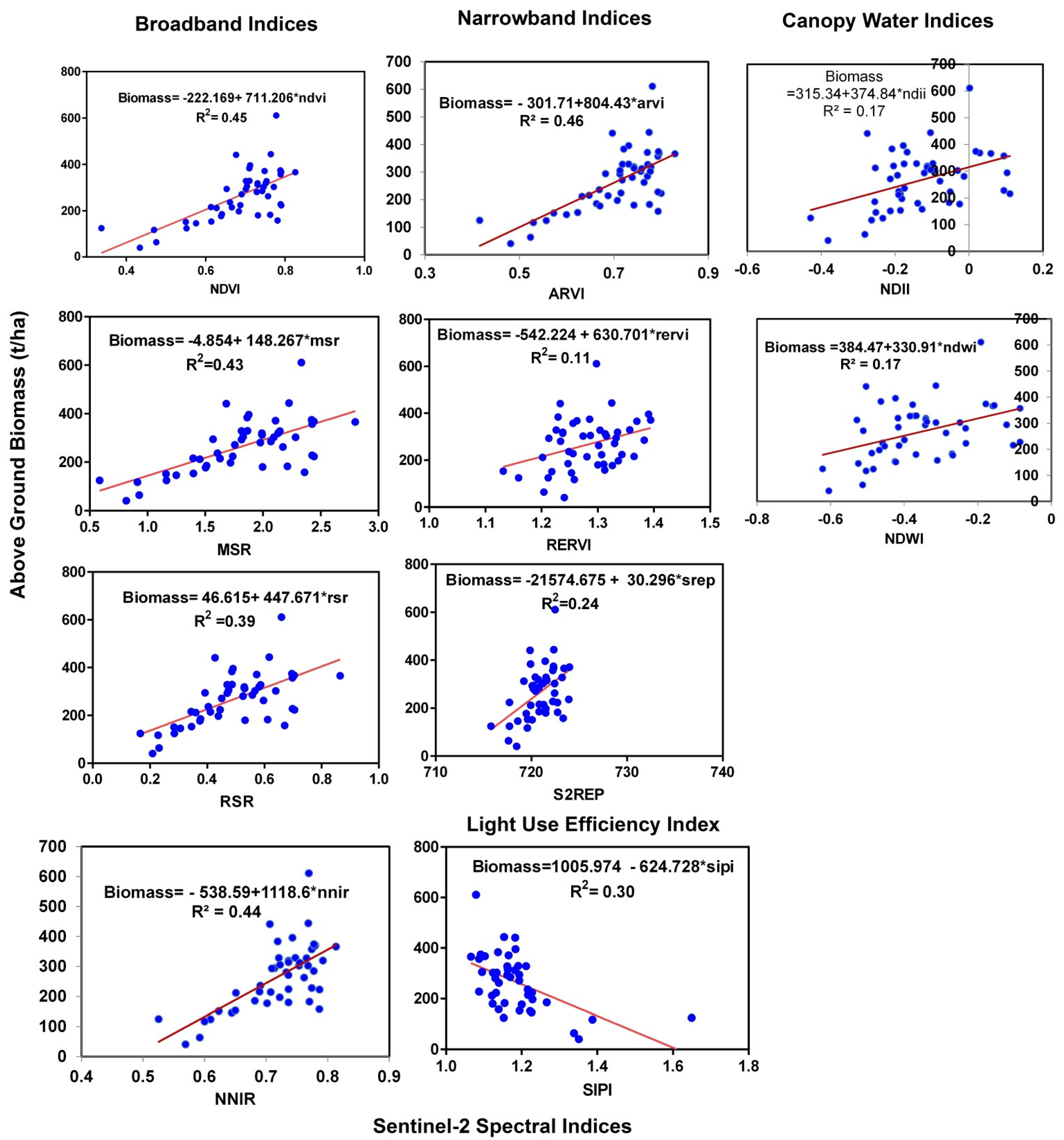
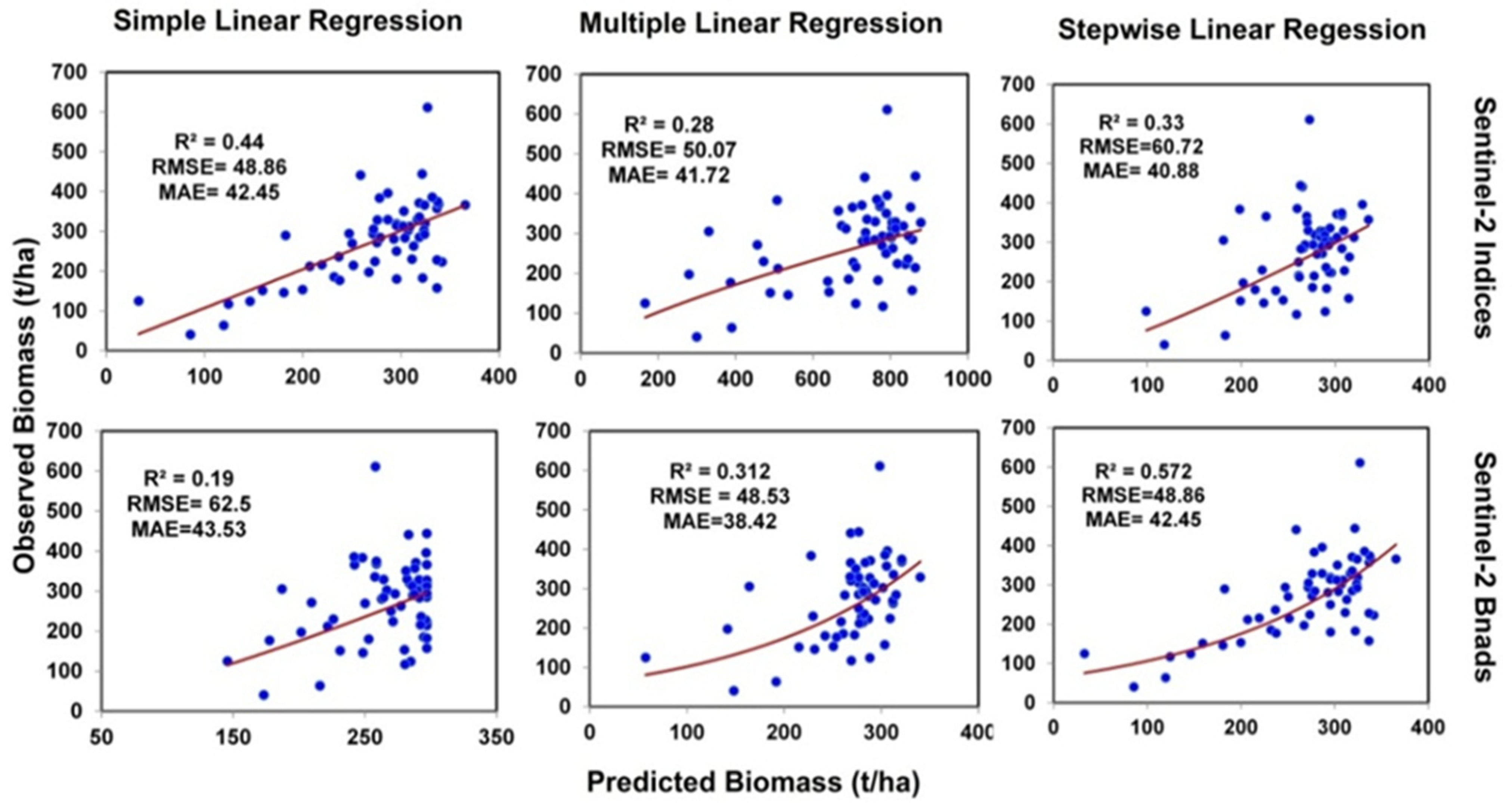
3.2. Simple Linear Regression

Among the four broadband indices (Figure 3), NDVI performed the best with an R² of 0.45, followed by the NNIR with an R² of 0.44. NDVI and NNIR linear relationships explained 45 and 44 percent of the data variations, respectively, while they were unable to describe 55% of the variation. The MSR also explained a similar data variation of 43% while of only 39% for RSR. Overall minor differences were observed in the behavior of these indices. As broadband indices use Red and NIR portions of the spectrum, these indices face saturation problems when an increase in canopy cover occurs. When vegetation canopy becomes denser in mature forests, saturation occurs. At this stage, broadband indices shoot up and cannot detect higher biomass [87]. Red absorption may reach the maximum in canopy cover approaching 100% and ultimately decrease in Red absorption relative to canopy increase. Such saturation in Red absorption may cause an unequal output from bands ratio (spectral analysis), leading to misleading biomass estimation. Narrow-band indices used in the present research were Red-edge Ratio Vegetation Index (RERVI), Atmospherically Resistant Vegetation Index (ARVI) and Sentinel-2 Red-edge position (S2REP). The highest correlation was found for ARVI with R² 0.46, followed by S2REP and RERVI with R² 0.24 and 0.11, respectively. The two narrow-band spectral indices (S2REP and RERVI) displayed poor correlation (performance) with the corresponding field-estimated biomass. Therefore, biomass estimation based on S2REP and RERVI will not give good results. SIPI positively correlated with biomass, and R² of 0.30 with a p-value of less than 0.01 was observed. Among the canopy water indices, the current study used the Normalized Difference Water Index (NDWI) and the Normalized Difference Infrared Index (NDII) for a linear relationship with biomass. The performance of both indices for AGB estimation was also similar, with an R² of 0.17 and a p-value of 0.003. The linear model of both indices has explained 30% of the data variations and demonstrated a good relationship with biomass. The resultant vegetation indices have been displayed in Supplementary Figure S2.

Similarly, the linear regression model of spectral bands showed that Band 1 (aerosol), Band 2 (Blue) and Band 4 (Red) demonstrated significant relationships with the biomass. In contrast, all the other bands’ relationships were insignificant. However, the R² values were not high when compared to spectral indices—Band 1 exhibited good performance compared to other bands (Band 2 and 4). The R² values were 0.12, 0.11 and 0.10 for Band 1, 2 and 3, respectively (Supplementary Figure S3).

3.3. Multiple and Stepwise Linear Regression

MLR models showed that ARVI has the highest correlation (0.67) with biomass compared to NDVI and NNIR, while the overall R² for the MLR model was 0.46 with a significance value of less than 0.0001 (

Table 4. Multiple linear regression of Sentinel-2 indices and bands versus biomass.

Correlations					Regression Summary
	Biomass	ARVI	NDVI	NNIR	R	0.683
Biomass	1.000				Adjusted R Square	0.430
ARVI	0.679	1.000			R Square	0.467
NDVI	0.675	0.995	1.000		Std. Error	82.225
NNIR	0.666	0.992	0.977	1.000	F-value	12.554
Model Equation Biomass = 2678.24*ARVI − 773.59*NDVI − 1439.98*NNIR − 57.373					Sig	0.000
	Biomass	B2	B4	B8A	R	0.476
Biomass	1.000				Adjusted R Square	0.173
B2	−0.342	1.000			R Square	0.227
B4	−0.320	0.963	1.000		Std. Error	99.015
B8A	−0.042	0.743	0.788	1.000	F-value	4.209
Model Equation Biomass = −2652.669*B2 − 1600.920*B4 + 674.487*B8A + 263.281					Sig	0.011

). The overall MLR R² has shown an increase in correlation compared to simple linear regression. Regarding the MLR model between the spectral bands and biomass, three rounds were selected on the basis of the significance value, which includes Band 2 (Blue), Band 4 (Red) and Band 8A (NIR). The overall correlation was 0.22, which has increased compared to the linear model of spectral bands and biomass. Band 2 has the highest correlation (0.34) among the spectral bands with biomass.

SLR showed that nine spectral bands were regressed against field AGB; however, Band 1 (aerosol) and Band 7 (Red-edge third band) were selected in the final regression model because these were significant (

Table 5. Stepwise regression of Sentinel-2 indices and bands versus biomass.

Variables			Correlations					Regression Summary
Entered	Removed	Sig		Biomass	ARVI	NDVI	NNIR	R	0.679
ARVI		0.000	Biomass	1.000				Adjusted R Square	0.449
	NDVI	0.990	ARVI	0.679	1.000			R Square	0.461
	NNIR	0.614	NDVI	0.675	0.995	1.000		Std. Error	80.830
			NNIR	0.666	0.992	0.977	1.000	F-value	38.469
Model Equation: Biomass = 804.433*ARVI − 301.711 + e								Sig	0.000
Sentinel-2 Bands and Biomass Stepwise Regression
Variables			Correlations					Regression Summary
Entered	Removed	Sig		Biomass	B1	B7		R	0.460
B1		0.000	Biomass	1				R Square	0.211
B7		0.037	B1	−0.359	1			Adjusted R Square	0.176
	B2	0.391	B7	−0.038	0.688	1		Std. Error	98.86
	B3	0.239	Model Equation Biomass = −6933.716*B1 + 569.194*B7 + 248.559					F-value	5.89
	B4	0.314						Sig	0.005
	B5	0.256
	B6	0.365	Method/decision for variable selection: Criteria: Probability-of-F-to-enter ≤0.050, Probability-of-F-to-remove ≥0.100
	B8A	0.537
	B11	0.365
	B12	0.470

). Similarly, when the best three spectral indices (NNIR, ARVI and NDVI) were regressed with biomass, only the ARVI was selected in the final model. The other indices were insignificant, with a p-value greater than 0.05. The overall R2 for the SLR model was 0.46, similar to that of the multiple linear models. Regarding single-band correlation among the spectral bands, Band 1 has the highest correlation (−0.35) with biomass.

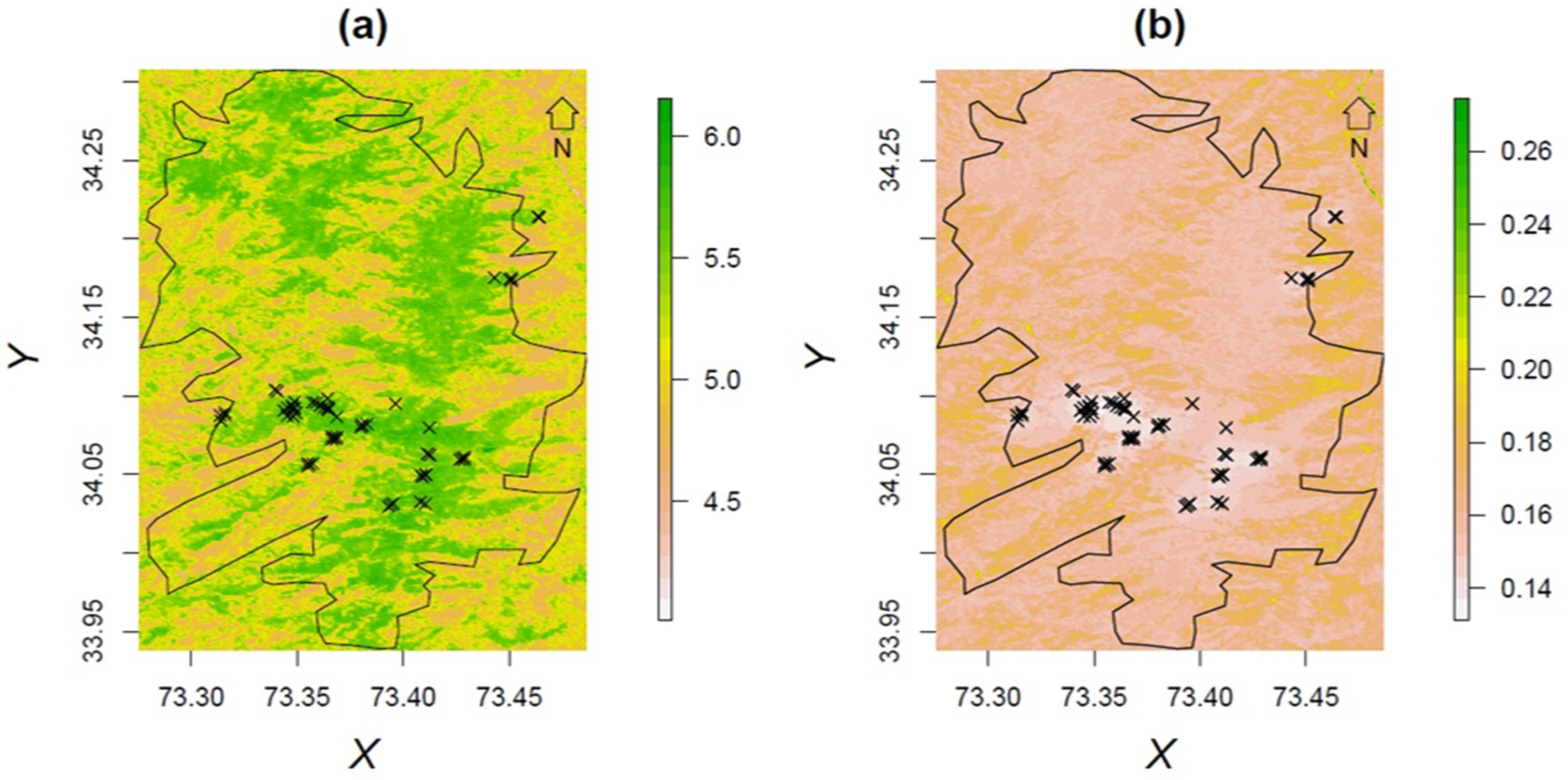
3.4. Geo-Statistical Biomass Estimation

All the explanatory variables (bioclimatic, topographic and demographic) were correlated with biomass. The distance to settlements, ARVI and annual precipitation were significantly associated with biomass, while other variables were insignificant (Supplementary Table S2). ARVI was strongly correlated to biomass with a p-value of less than 0.01. At the same time, the distance to settlements and annual precipitation was strongly associated with a p-value of less than 0.05. All other variables have a significance greater than 0.05, which means that a more significant p-value suggests that changes in explanatory variables will not significantly change the response variable. Some variables, such as ARVI, settlements, slope and precipitation, were also strongly correlated. These mutual correlations may affect model performance (Supplementary Table S2).

Stepwise linear regression models (SLRMs) were developed in R-Studio using biomass and all explanatory variables (

Table 6. Stepwise linear regression model for kriging.

Backward Selection (R2 0.42)				Forward Selection (R2 0.46)
	Estimate	Std. Error	p-Value		Estimate	Std. Error	p-Value
Intercept	185.390	109.91	0.097.	Intercept	74.31	56.71	0.195
Settlements	0.0381	0.0227	0.098.	ARVI	333.6	92.51	0.00064 ***
ARVI	275.11	96.160	0.005 **
Annual Temp	−1.10	0.7824	0.163
Model Equation: Biomass = 275.11*ARVI + 185.390				Model Equation: Biomass = 333.6*ARVI + 74.31
Signif. codes: 0.001 ‘**’ 0.01 ‘*’ 0.05 ‘.’ 0.1				Signif. codes: 0 ‘***’ 0.001 ‘**’ 0.01 ‘*’ 0.05

). SLRMs were evaluated in two directions of selection, namely (1) forward selection and (2) backward selection. The “forward” SLRM started with biomass and added all explanatory variables. At the same time, “backwards” SLRM took biomass and all explanatory variables and successively removed those variables with low importance. Backwards, the AIC value for the overall model started at 727.92 and stepwise while removing low-importance variables and ending at 716.59 in eight steps. The final step left with three variables (distance to settlements, ARVI and annual temperature), but only ARVI was enormously significant (p-value of 0.005) for biomass prediction. Forward selection starts with AIC 726.81 for the whole model (all variables) and ends at 716.67 in the second step with correlation (R² = 0.46).The forward selection resulted in a very strongly significant value (less than 0.000) for ARVI, and was therefore considered to be the best model as compared to the “backward” selection (Table 6). The forward selection model was considered best for prediction and used kriging to interpolate biomass throughout Galiesreserved forests. The kriging output biomass map depicts accurate biomass mapping similar to the Sentinel-2 image; however, kriging mapping comes with additional variance and uncertainty information about biomass prediction (Figure 4).

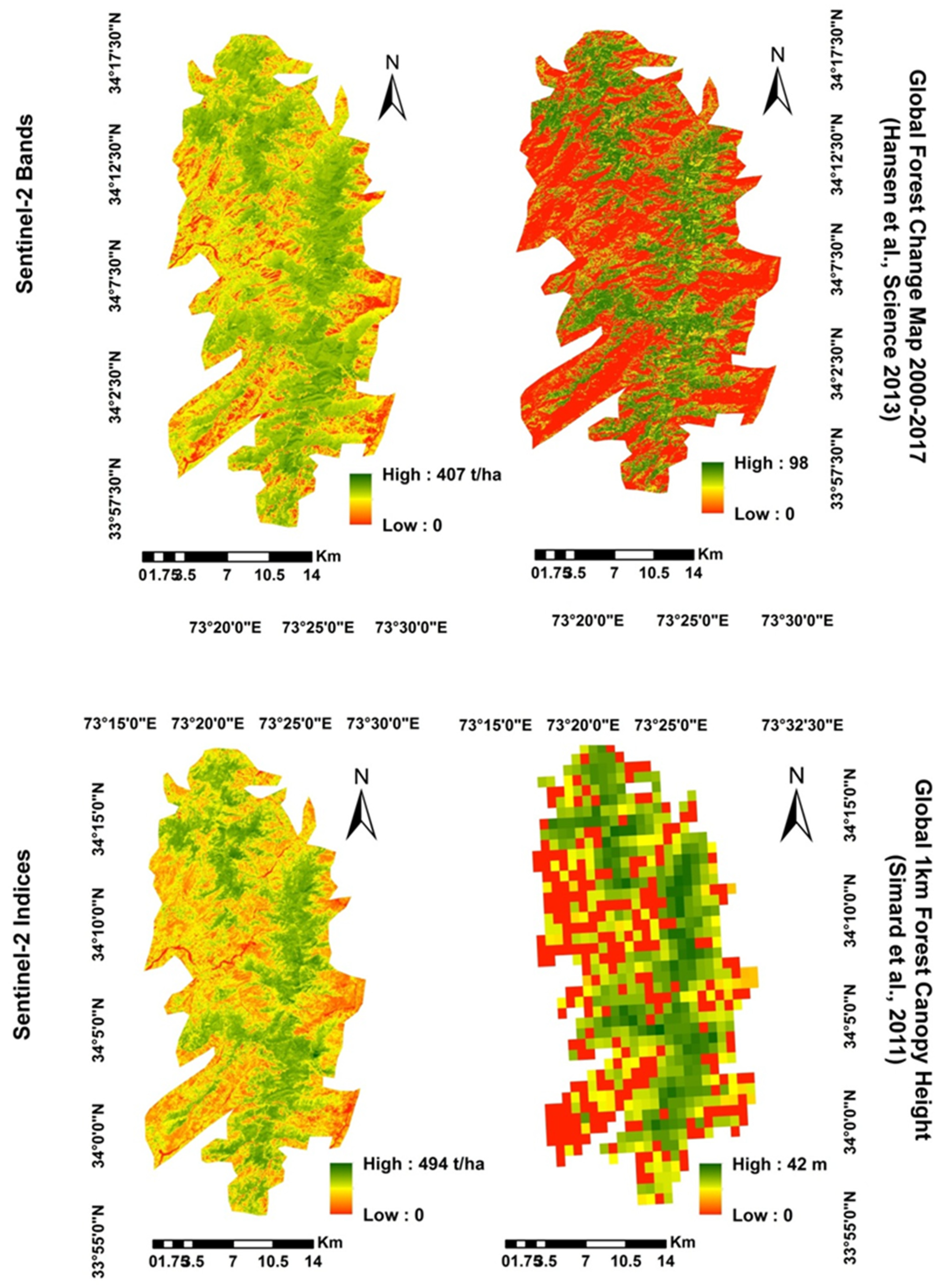
3.5. Model Accuracy and Biomass Mapping

The results show that the multiple linear regression model of the bands with biomass has the lowest RMSE (48.53) and MAE (38.42), and is therefore considered best for biomass estimation. However, among the three index models, the best was the stepwise model (ARVI), with RMSE and MAE values of 48.86 and 42.45, respectively (

Table 7. Accuracy assessment of AGB models.

Model	Regression	RMSE	MAE
Biomass = −301.710 + 804.432*arvi	Simple Linear	48.86	42.45
Biomass = 2678.24*ARVI − 773.59*NDVI − 1439.98*NNIR − 57.373	Multiple Linear	50.07	41.72
Biomass = 804.433*ARVI − 301.711	Stepwise Linear	48.86	42.45
Biomass = 297.40 − 3940.85*B1	Simple Linear	62.5	43.53
Biomass = −2652.669*B2 − 1600.920*B4+674.487*B8A + 263.281	Multiple Linear	48.53 *	38.42 *
Biomass = −6933.716*B1 + 569.194*B7 + 248.559	Stepwise Linear	60.72	40.88
‘ * ’ indicates the best regression model with least RMSE and MAE values

). The predicted biomass of all these models was correlated with observed biomass for inventory plots, as shown in Figure 5.The stepwise linear model of indices has the highest R² value (0.57), while the lowest R² value (0.19) was observed in a simple linear model of bands (band 1). The biomass maps were developed using linear (multiple and stepwise) regression. The results show that the lowest total biomass was predicted by a stepwise and straightforward linear model of ARVI.

In contrast, the highest forest cover was predicted by the Band 1 model of simple linear regression (Figure 3). The results show that biomass prediction by our best models has similar spatial distribution compared to Global Forest Cover datasets (Figure 6). Scatterplots of GFCC map versus the Sentinel-2 band’s map and the Sentinel-2 indices map displayed a better correlation with R² 0.20 and 0.25, respectively (Supplementary Figure S4a,c). On the other hand, the relationship of the GFCH map versus the Sentinel-2 band’s map and Sentinel-2 indices displayed a weak correlation with R2 0.16 and 0.16, respectively (Supplementary Figure S4b,d).

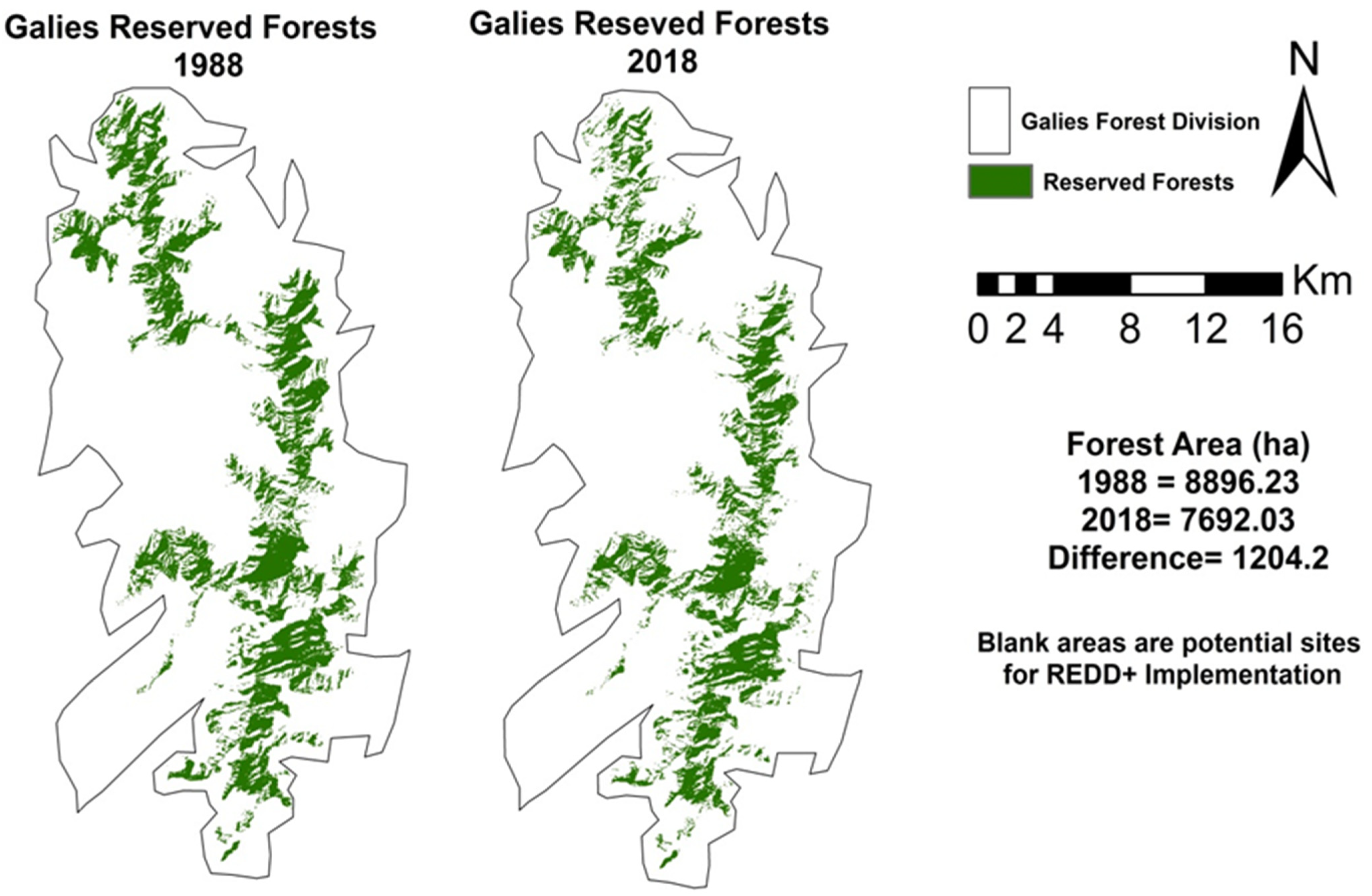
3.6. Potential Sites for REDD+ Implementation

The Landsat-5 and Landsat-8 images NDVI were reclassified with a threshold of 0.22 to 0.72 per output range.The results show that in 1988, the forest area was 8896.23 ha, while it was reduced to 7692.03 ha in 2018 (Figure 7). The Landsat NDVI output areas (both in 1988 and 2018) were smaller than when compared with departmental reports. This is because the smaller size of deforestation was not detected by Landsat and can be differentiated by high-resolution data. The difference in area between 1988 and 2018 was 1204.2 ha, which was less when compared to the departmental blank area (1610 ha). However, it is clear that the overall forest area was reduced during 1988–2018, and the blank regions were observed in different compartments. In the context of the REDD+ mechanism aimed primarily at reducing deforestation and forest degradation, the blank areas are the potential sites for REDD+ implementation in future projects. Moreover, the forest department has already allocated different working circles (W/Cs) for proper forest management. The main W/Cs of the Galies reserved forests are plantation W/C, improvement W/C, recreation W/C and production W/C; REDD+ can be implemented in these departmentally assigned W/Cs by reducing deforestation and controlling forest degradation in forested areas while ensuring the enhancement of forest carbon stocks in blank areas (Figure 7).

4. Discussion

4.1. Above-Ground Biomass Estimation

Previous studies reported similar results for above-ground biomass of moist temperate forests. Ahmed et al. [88] assessed biomass and carbon stocks of significant species (Abiespindrow, Pinus wallichiana, Cedrusdeodara and Piceasmithiana) in the coniferous forests district Dir. The research reported the mean AGB and mean AGC were 258.98 t/ha and 129.49 t/ha, respectively. Our results of mean AGB and AGC (274.29 t/ha and 128.92 t/ha) are consistent with the range of 215.5–468.2 t/ha AGB and of 107.8–234.1 t/ha AGC reported by Gairola et al. [89], who studied the tree biomass and carbon variations in a moist temperate forest, India. At the same time, a similar AGB range (360–440 t/ha) was published by Whittaker (1975), who gave an AGB estimation in a temperate forest. In other studies, Naeem et al. [90] estimated a mean AGB of 261 t/ha for the moist temperate forest of the study area, and Manan et al. [91] reported 287.9 t/ha AGB in adjoining moist temperate forests in Pakistan. Likewise, Dar [92] estimated the AGB of moist temperate forests in the adjacent Kashmir Himalaya and reported a mean AGB of 282 t/ha. The Intergovernmental Panel on Climate Change (IPCC) has reported a generic AGB range of 220–295 t/ha for the temperate forest, which is similar to our findings. However, in contrast to this study’s findings, some researchers estimated lower AGB, such as Khan et al. [93] who reported that the mean AGB for the moist temperate forests was 148.7 t/ha. Khan et al. [94] said that the average AGB was of 144.5 t/ha in the ecotone of sub-tropical pine and moist temperate forest and Ali et al. [95] reported an average AGB of 90.5 t/ha for temperate forests. Considering the findings of [90], forest stand structure significantly affects the AGB estimation. Higher stand density and species richness displayed higher AGB in a temperate forest in Pakistan. The present research area comprises higher stand density and species richness which contribute to higher AGB [96]; therefore, a higher mean AGB has been estimated (i.e., 274.29 t/ha) compared to other studies.

4.2. Sentinel-2 Spectral Indices for AGB Estimation

The present study computed spectral indices (including ARVI) derived from the Sentinel-2 images, and ARVI was the best index selected for AGB estimation and mapping. Lu (2005) studied the impact of forest structure attributes in AGB estimation using Landsat TM data and found that MLR models were better than simple regression for biomass estimation models. The author of [97] has reviewed various remote sensing and geo-statistical techniques for biomass estimation. The study described the performance of MLR as compared to linear regression models for biomass estimation. The author of [98] has compared various vegetation indices (NDVI, SAVI, MSAVI, GNDVI, TVI, DVI, etc.) for vegetation cover estimation. The MLR model used by Clerici et al. [99] derived spectral indices from GeoEye-1 and Pleiades-1A, developed a linear regression model between in-situ AGB data and spectral index and reported RVI has the most satisfactory performance (R² = 0.58) for AGB mapping. Basso et al. [100] utilized spectral indices (NDVI, SR and SAVI) and spectral bands of WorldView-2 image for AGB estimation and reported that NDVI and Band 1(Coastal) showed good correlation at (0.88) and (−0.10), respectively. In another study by Fuchs et al. [101], a multiple linear regression model was developed using spectral bands and indices against AGB data. The study reported that ARVI and Band 1, derived from Quickbird images, showed promising results with correlations of 0.50 and 0.58, respectively. Khan et al. [93] reported that RERVI derived from Sentinel-2 data was the best index for AGB estimation. Imran et al. [102] used Red-edge and canopy water indices (RENDVI, NDWI and NDII) computed from Sentinel-2 images. The stepwise regression model demonstrated NDWI as the best index with an R² of 0.46 for AGB estimation, whereas the Normalized Difference Index (DVI) and the Enhanced Vegetation Index (EVI) derived from Sentinel-2 images also showed promising results for AGB estimation [103]. Similarly, Imran et al. [104] showed that red-edge band-based vegetation indices of Sentinel-2 performed better (R² = 0.64) in estimating AGB compared to broadband spectral indices. Likewise, in addition to Sentinel-2 indices AGB models, other machine learning methods, such as random forest, support vector regression and geographically weighted regression, may enhance the accuracy of AGB estimates.Regarding geo-statistical AGB prediction, comprehensive field data of temperature, precipitation, soil type, soil moisture, soil nutrients, soil organic carbon, topography, forest opening, specie composition and density may improve AGB prediction.

4.3. Geo-Statistical Kriging-Based AGB Estimation

This research used ordinary kriging as a geo-statistical interpolation method to estimate and map AGB over the study area. The results show that the performance of ordinary kriging to predict AGB was consistent with the spectral index-based AGB estimation, and ARVI was selected as the best index for AGB mapping. However, significant limitations in geo-statistical interpolation were the spatial distribution of forest inventory data and usage of secondary data such as allometric equations for AGB estimation, DEM data, bioclimatic data and demographic data [105]. As the forest cover extended over a complex mountainous landscape, considered a discontinued variable, forest inventory data exhibited lower autocorrelation, resulting in lower accuracy for the ordinary kriging method [42] and causing overfit as it does not explain effectively [106]. Kriging interpolation accuracy increases with the addition of explanatory variables measured during primary data collection [72]. Similarly, adding co-variables for AGB prediction at unknown locations in co-kriging improves accuracy and surpasses ordinary kriging [49]. Likewise, Reich et al. [107] reported that the spatial independency of forest attributes makes the data difficult to model spatial variability with the ordinary kriging method. Moreover, in AGB prediction in topographically complex forest vegetation, Su et al. [49] reported that co-kriging (combined with random forests) was the best interpolation method compared to ordinary kriging and simple regression models. In consistency with the findings of this study, Tuominen et al. [108] reported that geo-statistical interpolation does not enhance the accuracy of forest volume prediction when combined with spectral data of satellite images. Similarly, in another study, Freeman and Moisen [105] assessed kriging as a technique to enhance AGB prediction and reported no significant improvement in map accuracy. Furthermore, they reported a higher statistical error in kriging interpolation compared to direct radiometric relationships using spectral indices. Likewise, conducting intensive insitu forest sampling and integrating different supplementary explanatory variables in geo-statistical modeling should be used for the improved accuracy of AGB estimation [42].

4.4. Comparison of Remote Sensing and Geo-Statistical Techniques for AGB Estimation

The present study compared the AGB maps developed from linear regression models based on remote sensing data with the ordinary kriging method to predict and map AGB at unknown locations. However, the accuracy of the geo-statistical method was almost similar to the remote sensing technique. SLR for selecting significant explanatory variables showed a correlation (R² = 0.43) for ARVI, slightly lower than the remote sensing technique (R² = 0.46). Previous studies showed that geo-statistical methods had shown higher accuracy than remote sensing techniques; however, in the case of this research, limited data of topographic, edaphic, climatic and anthropogenic/demographic factors also affect the accuracy of the kriging technique. Similarly, kriging accuracy also depends upon the spatial distribution and heterogeneity of the AGB field plots [43]. Moreover, randomness and representative field plots are also vital for accurate AGB interpolation. Practically, ordinary kriging requires more insitu sample plot data to predict AGB at unknown locations [109]. The present study may have fewer sample plots or insufficient spatial distribution. Therefore, the AGB prediction map has shown a slightly lesser accuracy than remote sensing data [110]. In order to find the optimal interpolation method for a particular forest type, repeated data collection is based on previous field information/method with minimum errors [110]. In another study, regression kriging exhibited better results predicting carbon stocks in fragmented forest biomes than ordinary kriging and co-kriging [111]. Yadav and Nabdy [109] compared geo-statistical interpolation methods and reported that K-nearest neighbor (kNN) performed better than co-kriging because it is a non-parametric approach. Benitez et al. [75] said that integrating spectral indices derived from higher resolution satellite images with geo-statistical kriging improves the AGB prediction accuracy, whereas the present study used Sentinel-2 images with a medium spatial resolution of 10 m; therefore, the usage of higher resolution images may enhance the accuracy of the kriging method. The interpolation of AGB based on geostatistics significantly depends on spatial patterns and spatial autocorrelations, whereas spectral indices derived from satellite images mainly do not explain the spatial heterogeneity of bioclimatic and edaphic factors, as established by Maselli and Chiesi [112]. Therefore, an integrated prediction model of remote sensing data and geo-statistical techniques significantly improves the AGB estimation and mapping [113]. The present study has some limitations, such as using third-party allometric equations for AGB estimation, which is one of the significant limitations in AGB accuracy. Locally developed standard allometric equations are critical for AGB estimation and variations within the stand. Furthermore, the lack of field-based data (topographic, bioclimatic, soil type) is another main limitation for AGB prediction by kriging interpolation. Therefore, the accuracy of AGB is affected by third-party data. Similarly, despite the high spatial resolution, Sentinel-2 imagery has some limitations. Variations of biomass in the dense canopy in moist temperate forests and forest degradation may not be efficiently quantified by Sentinel-2 images (i.e.,10 m spatial resolution).

4.5. Present Research Contribution to REDD+ MRV

The main goal of the REDD+ MRV system is to explore the reliable, accurate and economical technique for AGB estimation. The present study explored the potential of Sentinel-2 images and derived spectral indices for carbon stock mapping; therefore, it may contribute to the regional MRV system of the national REDD+ mechanism, particularly in the SLMS of NFMS. For instance, AGB modeling and carbon stocks mapping based on spectral indices on local scale, provide additional monitoring data to the national REDD+ SLMS [39,40,93]. Moreover, keeping in view the results of this pilot research, open-source Sentinel-2 images (with medium resolution) may be used for wall-to-wall coverage of REDD+ activities, which may give better results with enhanced accuracy. Pacheco-Pascagaza [28] and Roberts [114] compared to Landsat images (with lower resolution) used by the NFMS. Simonetti et al., [115] developed a Sentinel-2 web platform for the MRV system of REDD+ implementation, where the NFMSs of developing countries easily access and acquire Sentinel-2 time series data with high temporal resolution. Furthermore, the presence of Red-edge bands in Sentinel-2 multispectral images is very useful to minimize the saturation issues in AGB estimation and monitoring [115]. Likewise, presently national SLMSsare working with LULC classification and mapping using random forests [14]; spectral indices explored in this study may be incorporated as explanatory variables for AGB mapping and carbon accounting of SLMS at a regional scale. To strengthen the existing NFMS ((https://www.nfmspak.org/) (accessed on 19 January, 2023)), AGB modeling based on vegetation indices and insitu forest inventory may be integrated in order to provide local carbon estimates online. On the other hand, the present study also explored geostatistical interpolation (ordinary kriging) of AGB estimation using spectral index, topographic, demographic and climatic variables. Such geostatistical interpolation techniques may be used in regional carbon estimates/action results in the MRV system of REDD+ implementation [116], which not only increases the accuracy of carbon accounting but also provides integrated data of spatial covariance [117,118].

4.6. Limitations in AGB Modeling in Mountainous Areas

Accurate AGB modeling in the topographically diverse mountainous areas is always a challenging task and the present study’s modeling of AGB through Sentinel-2 spectral indices and geostatistical methods may be further improved with LiDAR with least uncertainty [119,120,121]. Landscape heterogeneity and AGB saturation may be reduced significantly with the fusion of pixel-sized LiDAR data and AGB spectral predictors [122,123,124]. The present study used predictor variables derived from STRM DEM of 30 m resolution for AGB modeling with acceptable accuracy [125]; however, high-resolution DEM variables may improve accuracy. Sliwinski et al. [84] explored high-resolution DEM (1 m) extracted from LiDAR data for watershed modeling using a SWAT model and used resampling methods based on pixel-based summary statistics (measure of central tendency) for a progressive decrease in DEM resolution. This study showed a high-resolution DEM decrease in precision and produced erroneous results in watershed modeling compared to high-resolution DEM. This study suggested that such a resampling technique based on LiDAR DEM is the most apposite for the modeling of catchment areas along the altitudinal gradients. However, the acquisition of ubiquitous cover of LiDAR data for large-area AGB estimation is costly and commercial [84]. Presently, in Pakistan, the use of LiDAR systemsis limited to smaller areas; therefore, a LiDAR DEM-based analysis for AGB modeling was not considered, keeping in view expenses and the restricted scope of acquisition.

5. Conclusions

The use of remote sensing techniques for forest biomass and carbon stock estimation can be implemented with acceptable accuracy. Geo-statistical techniques also provide us with models for the spatial distribution of biomass. The main objectives of the present study were to explore the relationship between spectral bands and indices with biomass using simple, multiple and stepwise linear regression using Sentinel-2 images and geo-statistical techniques and to compare the resultant biomass maps with global datasets to explore various potential sites for REDD+ implementation. The results show that ARVI was the best index among all indices, with a higher R² (0.67) than the rest of the spectral index. MLR showed that the indices model with ARVI, NNIR and NDVI was significant with an R² of 0.46, while Band 2 (Blue), Band 4 (Red) and Band 8A (NIR) models have satisfactory performance with an R² of 0.22. Similarly, SLR exhibited almost similar correlation for indices and bands with an R² of 0.46 and an R² of 0.21, respectively. The MLR of bands with biomass has the lowest RMSE (48.53) and MAE (38.42) and is therefore considered best for biomass estimation. Furthermore, the geo-statistical technique, the distance to settlements, ARVI and annual precipitation were significantly correlated with biomass, while other variables were insignificant. However, in the stepwise selection, the forward section resulted in a very significant value (less than 0.000) for ARVI and was therefore considered the best model for AGB interpolation using ordinary kriging compared to “backward” selection. Comparative analysis showed that remote sensing estimation was better for biomass than geostatistics. Regarding REDD+ implementation potential sites, Landsat images showed a decrease in forest cover (1988—2018). The forest area was 8896.23 ha in 1988. It was reduced to 7692.03 ha in 2018; the blank areas are potential sites for future projects. Moreover, the accuracy of Sentinel-2-derived indices was affected in higher-density areas because the AGB saturation issue lowered the prediction accuracy. However, AGB estimation may be improved by using multi-source RS data, or data fusion may give better results such as Sentinel-2 may be integrated with Sentinel-1, Sentinel-3, PALSAR-2 and LiDAR. Furthermore, using the rest of the Sentinel-2 bands is recommended to compute spectral indices and their potential for AGB estimation. The present study concluded that as a state-of-the-art sensor, the Sentinel-2 data have great potential for forest biomass and carbon stocks estimation and can be implemented with acceptable accuracy.

References

1. Simula, M.; Mansur, E. A global challenge needing local response. Unasylva 2011, 62, 3–7. [Google Scholar]
2. Eggleston, S.; Buendia, L.; Miwa, K.; Ngara, T.; Tanabe, K. Volume 4: Agriculture, forestry and other land use. In 2006 IPCC Guidelines for National Greenhouse Gas Inventories; Institute for Global Environmental Strategies (IGES): Hayama, Japan, 2006. [Google Scholar]
3. Fry, I. Reducing Emissions from Deforestation and Forest Degradation: Opportunities and Pitfalls in Developing a New Legal Regime. Rev. Eur. Community Int. Environ. Law 2008, 17, 166–182. [Google Scholar] [CrossRef]
4. UNFCCC. Factsheet: Reducing Emissions from Deforestation in Developing Countries: Approaches to Stimulate Action. 2011. Available online: http://unfccc.int/files/press/backgrounders/application/pdf/fact_sheet_reducing_emissions_from_deforestation.pdf (accessed on 19 January 2019).
5. Page, P. Report of the Ad Hoc Working Group on Long-Term Cooperative Action under the Convention on the First Part of Its Fifteenth Session, Held in Bonn from 15 to 24 May 2012; United Nations: New York, NY, USA, 2012. [Google Scholar]
6. Herold, M.; Skutsch, M. Monitoring, reporting and verification for national REDD + programmes: Two proposals. Environ. Res. Lett. 2011, 6. [Google Scholar] [CrossRef]
7. Skutsch, M.M.; Torres, A.B.; Mwampamba, T.H.; Ghilardi, A.; Herold, M. Dealing with locally-driven degradation: A quick start option under REDD+. Carbon Balance Manag. 2011, 6, 16. [Google Scholar] [CrossRef]
8. Maniatis, D.; Mollicone, D. Options for sampling and stratification for national forest inventories to implement REDD+ under the UNFCCC. Carbon Balance Manag. 2010, 5, 9. [Google Scholar] [CrossRef] [PubMed]
9. Köhl, M.; Neupane, P.R.; Mundhenk, P. REDD+ measurement, reporting and verification–A cost trap? Implications for financing REDD+ MRV costs by result-based payments. Ecol. Econ. 2020, 168, 106513. [Google Scholar] [CrossRef]
10. Singh, N.; Finnegan, J.; Levin, K.; Rich, D.; Sotos, M.; Tirpak, D.; Wood, D. MRV 101: Understanding measurement, reporting, and verification of climate change mitigation. World Resour. Inst. 2016, 4–5. [Google Scholar]
11. Penman, J.; Gytarsky, M.; Hiraishi, T.; Krug, T.; Kruger, D.; Pipatti, R.; Buendia, L.; Miwa, K.; Ngara, T.; Tanabe, K. Definitions and Methodological Options to Inventory Emissions from Direct Human-Induced Degradation of Forests and Devegetation of Other Vegetation Types; IPCC National Greenhouse Gas Inventories Programme-Technical Support Unit: Kanagawa, Japan, 2003; p. 32. [Google Scholar]
12. Shrestha, S.; Karky, B.S.; Karki, S. Case Study Report: REDD+ Pilot Project in Community Forests in Three Watersheds of Nepal. Forests 2014, 5, 2425–2439. [Google Scholar] [CrossRef]
13. Oy, A.; Iqbal Mohammad, W.; Muhhamad Humza, W.; Usman Akram, W.; Shaheen Arief, W. WWF-Pakistan. In National Forest Monitoring System-Measurement, Reporting and Verification (MRV) System for Pakistan; MoCC/National REDD+ Office: Islamabad, Pakistan, 2018. [Google Scholar]
14. Mumtaz, F.; Li, J.; Liu, Q.; Tariq, A.; Arshad, A.; Dong, Y.; Zhao, J.; Bashir, B.; Zhang, H.; Gu, C.; et al. Impacts of Green Fraction Changes on Surface Temperature and Carbon Emissions: Comparison under Forestation and Urbanization Reshaping Scenarios. Remote. Sens. 2023, 15, 859. [Google Scholar] [CrossRef]
15. Mitchell, A.L.; Rosenqvist, A.; Mora, B. Current remote sensing approaches to monitoring forest degradation in support of countries measurement, reporting and verification (MRV) systems for REDD+. Carbon Balance Manag. 2017, 12, 1–22. [Google Scholar] [CrossRef] [PubMed]
16. Puliti, S. Analyses of the Feasibility of Participatory REDD+ MRV Approaches to Lidar Assisted Carbon Inventories in Nepal. Master Thesis, Sveriges Lantbruksuniversitet, Uppsala, Sweden, 2012. [Google Scholar]
17. Dangi, R. REDD+: Issues and challenges from a Nepalese perspective. Clim. Change UNFCCC Negot. Process 2012, 61. [Google Scholar]
18. Skutsch, M.; Mccall, M.; Karky, B.; Zahabu, E.; Guarin, G. Case studies on measuring and assessing forest degradation. Community Meas. Carbon Stock Change REDD For. Resour. Assess. Work. Pap. 2009, 156. [Google Scholar]
19. Scheyvens, H. Community-Based Forest Monitoring for REDD+: Lessons and Reflflections from the Field; Institute for Global Environmental Strategies: Kanagawa Prefecture, Japan, 2012. [Google Scholar]
20. Danielsen, F.; Skutsch, M.; Burgess, N.; Jensen, P.; Andrianandrasana, H.; Karky, B.; Lewis, R.; Lovett, J.; Massao, J.; Ngaga, Y. At the heart of REDD+: A role for local people in monitoring forests? Conserv. Lett. 2011, 4, 158–167. [Google Scholar] [CrossRef]
21. Musinguzi, G.B. Assessing In-House Capacity for Participatory GIS in Community-Based Measuring Reporting and Verification (MRY) Systems in Uganda; Makerere University: Kampala, Uganda, 2022. [Google Scholar]
22. Murthy, M.S.R.; Wesselman, S.; Gilani, H. Multi-Scale Forest Biomass Assessment and Monitoring in the Hindu Kush Himalayan Region: A Geospatial Perspective; International Centre for Integrated Mountain Development (ICIMOD): Lalitpur, Nepal, 2015. [Google Scholar]
23. Vashum, K.T.; Jayakumar, S. Methods to estimate above-ground biomass and carbon stock in natural forests-a review. J. Ecosyst. Ecography 2012, 2, 1–7. [Google Scholar] [CrossRef]
24. Ravindranath, N.H.; Ostwald, M. Carbon Inventory Methods: Handbook for Greenhouse Gas Inventory, Carbon Mitigation and Roundwood Production Projects; Springer Science & Business Media: Berlin/Heidelberg, Germany, 2007; Volume 29. [Google Scholar]
25. Ismail, I.; Sohail, M.; Gilani, H.; Ali, A.; Hussain, K.; Hussain, K.; Karky, B.; Qamer, F.; Qazi, W.; Ning, W. Forest inventory and analysis in Gilgit-Baltistan: A contribution towards developing a forest inventory for all Pakistan. Int. J. Clim. Change Strateg. Manag. 2018, 10, 616–631. [Google Scholar] [CrossRef]
26. Du, L.; Zhou, T.; Zou, Z.; Zhao, X.; Huang, K.; Wu, H. Mapping Forest Biomass Using Remote Sensing and National Forest Inventory in China. Forests 2014, 5, 1267–1283. [Google Scholar] [CrossRef]
27. Rahm, M.; Cayet, L.; Anton, V.; Mertons, B. Detecting forest degradation in the Congo Basin by optical remote sensing. In Proceedings of the ESA’s Living Planet Symposium, Edinburgh, UK, 9–13 September 2013. [Google Scholar]
28. Mermoz, S.; Le Toan, T.; Villard, L.; Réjou-Méchain, M.; Seifert-Granzin, J. Biomass assessment in the Cameroon savanna using ALOS PALSAR data. Remote. Sens. Environ. 2014, 155, 109–119. [Google Scholar] [CrossRef]
29. Santos, M.M.; Machado, I.E.S.; Carvalho, E.V.; Viola, M.R.; Giongo, M. Estimativa de parâmetros florestais em área de cerrado a partir de imagens do sensor landsat 8. Floresta 2017, 47, 75. [Google Scholar] [CrossRef]
30. Jakubauskas, M.E.; Price, K. Regression-Based Estimation of Lodgepole Pine Forest Age from Landsat Thematic Mapper Data. Geocarto Int. 2000, 15, 21–26. [Google Scholar] [CrossRef]
31. Potter, C.; Dolanc, C. Thirty Years of Change in Subalpine Forest Cover from Landsat Image Analysis in the Sierra Nevada Mountains of California. For. Sci. 2016, 62, 623–632. [Google Scholar] [CrossRef]
32. Gu, C.; Clevers, J.G.; Liu, X.; Tian, X.; Li, Z.; Li, Z. Predicting forest height using the GOST, Landsat 7 ETM+, and airborne LiDAR for sloping terrains in the Greater Khingan Mountains of China. ISPRS J. Photogramm. Remote. Sens. 2018, 137, 97–111. [Google Scholar] [CrossRef]
33. Xiwen, L.; Yinghui, Z.; Zhen, Z.; Qingbin, W. Forest Vegetation Classification of Landsat-8 Based on Rotation Forest. Available online: https://www.zhangqiaokeyan.com/academic-journal-cn_journal-northeast-forestry-university_thesis/0201261612122.html (accessed on 19 January 2019).
34. Asner, G.P.; Brodrick, P.; Philipson, C.; Vaughn, N.; Martin, R.; Knapp, D.; Heckler, J.; Evans, L.; Jucker, T.; Goossens, B. Goossens, Mapped aboveground carbon stocks to advance forest conservation and recovery in Malaysian Borneo. Biol. Conserv. 2018, 217, 289–310. [Google Scholar] [CrossRef]
35. Vesakoski, J.-M.; Nylén, T.; Arheimer, B.; Gustafsson, D.; Isberg, K.; Holopainen, M.; Hyyppä, J.; Alho, P. Arctic Mackenzie Delta channel planform evolution during 1983-2013 utilising Landsat data and hydrological time series. Hydrol. Process. 2017, 31, 3979–3995. [Google Scholar] [CrossRef]
36. Margono, B.A.; Turubanova, S.; Zhuravleva, I.; Potapov, P.; Tyukavina, A.; Baccini, A.; Goetz, S.; Hansen, M.C. Mapping and monitoring deforestation and forest degradation in Sumatra (Indonesia) using Landsat time series data sets from 1990 to 2010. Environ. Res. Lett. 2012, 7, 034010. [Google Scholar] [CrossRef]
37. Gizachew, B.; Solberg, S.; Næsset, E.; Gobakken, T.; Bollandsås, O.M.; Breidenbach, J.; Zahabu, E.; Mauya, E.W. Mapping and estimating the total living biomass and carbon in low-biomass woodlands using Landsat 8 CDR data. Carbon Balance Manag. 2016, 11, 13. [Google Scholar] [CrossRef]
38. Reimer, F.; Asner, G.P.; Joseph, S. Advancing reference emission levels in subnational and national REDD+ initiatives: A CLASlite approach. Carbon Balance Manag. 2015, 10, 5. [Google Scholar] [CrossRef]
39. Adan, M.S. Integrating Sentinel-2 Derived Vegetation Indices and Terrestrial Laser Scanner to Estimate Above-Ground Biomass/Carbon in Ayer Hitam Tropical Forest Malaysia; University of Twente: Enschede, The Netherlands, 2017. [Google Scholar]
40. Ali, A.; Ullah, S.; Bushra, S.; Ahmad, N.; Ali, A.; Khan, M. Quantifying forest carbon stocks by integrating satellite images and forest inventory data. Austrian J. For. Sci./Cent. Für Das Gesamte Forstwes. 2018, 135, 93–117. [Google Scholar]
41. Pandit, S.; Tsuyuki, S.; Dube, T. Estimating Above-Ground Biomass in Sub-Tropical Buffer Zone Community Forests, Nepal, Using Sentinel 2 Data. Remote. Sens. 2018, 10, 601. [Google Scholar] [CrossRef]
42. Viana, H.; Aranha, J.; Lopes, D.; Cohen, W.B. Estimation of crown biomass of Pinus pinaster stands and shrubland above-ground biomass using forest inventory data, remotely sensed imagery and spatial prediction models. Ecol. Model. 2012, 226, 22–35. [Google Scholar] [CrossRef]
43. Wai, P.; Su, H.; Li, M. Estimating Aboveground Biomass of Two Different Forest Types in Myanmar from Sentinel-2 Data with Machine Learning and Geostatistical Algorithms. Remote. Sens. 2022, 14, 2146. [Google Scholar] [CrossRef]
44. Silveira, E.M.; Santo, F.D.E.; Wulder, M.A.; Júnior, F.W.A.; Carvalho, M.C.; Mello, C.R.; Mello, J.M.; Shimabukuro, Y.E.; Terra, M.C.N.S.; Carvalho, L.M.T.; et al. Pre-stratified modelling plus residuals kriging reduces the uncertainty of aboveground biomass estimation and spatial distribution in heterogeneous savannas and forest environments. For. Ecol. Manag. 2019, 445, 96–109. [Google Scholar] [CrossRef]
45. Chatterjee, S.; Santra, P.; Majumdar, K.; Ghosh, D.; Das, I.; Sanyal, S.K. Geostatistical approach for management of soil nutrients with special emphasis on different forms of potassium considering their spatial variation in intensive cropping system of West Bengal, India. Environ. Monit. Assess. 2015, 187, 183. [Google Scholar] [CrossRef]
46. Pierce, K.B.; Ohmann, J.L.; Wimberly, M.; Gregory, M.J.; Fried, J. Mapping wildland fuels and forest structure for land management: A comparison of nearest neighbor imputation and other methods. Can. J. For. Res. 2009, 39, 1901–1916. [Google Scholar] [CrossRef]
47. Akhavan, R.; Kia-Daliri, H. Spatial variability and estimation of tree attributes in a plantation forest in the Caspian region of Iran using geostatistical analysis. Casp. J. Environ. Sci. 2010, 8, 163–172. [Google Scholar]
48. Chen, L.; Wang, Y.; Ren, C.; Zhang, B.; Wang, Z. Assessment of multi-wavelength SAR and multispectral instrument data for forest aboveground biomass mapping using random forest kriging. For. Ecol. Manag. 2019, 447, 12–25. [Google Scholar] [CrossRef]
49. Su, H.; Shen, W.; Wang, J.; Ali, A.; Li, M. Machine learning and geostatistical approaches for estimating aboveground biomass in Chinese subtropical forests. For. Ecosyst. 2020, 7, 64. [Google Scholar] [CrossRef]
50. Nizami, S.M. The inventory of the carbon stocks in sub tropical forests of Pakistan for reporting under Kyoto Protocol. J. For. Res. 2012, 23, 377–384. [Google Scholar] [CrossRef]
51. McRoberts, R.E.; Tomppo, E.O.; Næsset, E. Advances and emerging issues in national forest inventories. Scand. J. For. Res. 2010, 25, 368–381. [Google Scholar] [CrossRef]
52. Molto, Q.; Rossi, V.; Blanc, L. Error propagation in biomass estimation in tropical forests. Methods Ecol. Evol. 2012, 4, 175–183. [Google Scholar] [CrossRef]
53. Chave, J.; Andalo, C.; Brown, S.; Cairns, M.A.; Chambers, J.Q.; Eamus, D.; Fölster, H.; Fromard, F.; Higuchi, N.; Kira, T.; et al. Tree allometry and improved estimation of carbon stocks and balance in tropical forests. Oecologia 2005, 145, 87–99. [Google Scholar] [CrossRef]
54. Gao, X.; Li, Z.; Yu, H.; Jiang, Z.; Wang, C.; Zhang, Y.; Qi, L.; Shi, L. Modeling of the height–diameter relationship using an allometric equation model: A case study of stands of Phyllostachys edulis. J. For. Res. 2015, 27, 339–347. [Google Scholar] [CrossRef]
55. Gao, X.; Jiang, Z.; Guo, Q.; Zhang, Y.; Yin, H.; He, F.; Qi, L.; Shi, L. Allometry and Biomass Production of Phyllostachys Edulis Across the Whole Lifespan. Pol. J. Environ. Stud. 2015, 24, 511–517. [Google Scholar]
56. Angulo, C.E.P.; Vilanova, E.; Aguado, I.; Armenta, S.A.M.; Martínez, S. Carbon Emissions from Deforestation and Degradation in a Forest Reserve in Venezuela between 1990 and 2015. Forests 2017, 8, 291. [Google Scholar] [CrossRef]
57. Roxburgh, S.H.; Wood, S.W.; Mackey, B.; Woldendorp, G.; Gibbons, P. Assessing the carbon sequestration potential of managed forests: A case study from temperate Australia. J. Appl. Ecol. 2006, 43, 1149–1159. [Google Scholar] [CrossRef]
58. Sentinel, E. MSI—Level-2A Prototype Processor Installation and User Manual. Available online: https://sentinels.copernicus.eu/web/sentinel/user-guides/sentinel-2-msi/product-types/level-2a (accessed on 19 January 2019).
59. Gascon, F.; Bouzinac, C.; Thépaut, O.; Jung, M.; Francesconi, B.; Louis, J.; Lonjou, V.; Lafrance, B.; Massera, S.; Gaudel-Vacaresse, A.; et al. Copernicus Sentinel-2A Calibration and Products Validation Status. Remote Sens. 2017, 9, 584. [Google Scholar] [CrossRef]
60. Simard, M.; Pinto, N.; Fisher, J.B.; Baccini, A. Mapping forest canopy height globally with spaceborne lidar. J. Geophys. Res. Atmos. 2011, 116. [Google Scholar] [CrossRef]
61. Hansen, M.C.; Potapov, P.V.; Moore, R.; Hancher, M.; Turubanova, S.A.; Tyukavina, A.; Thau, D.; Stehman, S.V.; Goetz, S.J.; Loveland, T.R.; et al. High-Resolution Global Maps of 21st-Century Forest Cover Change. Science 2013, 342, 850–853. [Google Scholar] [CrossRef] [Green Version]
62. Jiang, Z.; Huete, A.R.; Didan, K.; Miura, T. Development of a two-band enhanced vegetation index without a blue band. Remote Sens. Environ. 2008, 112, 3833–3845. [Google Scholar] [CrossRef]
63. Chen, J.M. Evaluation of Vegetation Indices and a Modified Simple Ratio for Boreal Applications. Can. J. Remote Sens. 1996, 22, 229–242. [Google Scholar] [CrossRef]
64. Tehrani, N.A.; Naimi, B.; Jaboyedoff, M. Modeling current and future species distribution of breeding birds as regional essential biodiversity variables (SD EBVs): A bird perspective in Swiss Alps. Glob. Ecol. Conserv. 2021, 27, e01596. [Google Scholar] [CrossRef]
65. Huete, A.R. A soil-adjusted vegetation index (SAVI). Remote Sens. Environ. 1988, 25, 295–309. [Google Scholar] [CrossRef]
66. Kaufman, Y.J.; Tanre, D. Atmospherically resistant vegetation index (ARVI) for EOS-MODIS. IEEE Trans. Geosci. Remote Sens. 1992, 30, 261–270. [Google Scholar] [CrossRef]
67. Cao, Q.; Miao, Y.; Shen, J.; Yu, W.; Yuan, F.; Cheng, S.; Huang, S.; Wang, H.; Yang, W.; Liu, F. Improving in-season estimation of rice yield potential and responsiveness to topdressing nitrogen application with Crop Circle active crop canopy sensor. Precis. Agric. 2015, 17, 136–154. [Google Scholar] [CrossRef]
68. Guyot, G.; Baret, F. Utilisation de la haute resolution spectrale pour suivre l’etat des couverts vegetaux. Spectr. Signat. Objects Remote Sens. 1988, 279. [Google Scholar]
69. Penuelas, J.; Baret, F.; Filella, I. Semi-empirical indices to assess carotenoids/chlorophyll a ratio from leaf spectral reflectance. Photosynthetica 1995, 31, 221–230. [Google Scholar]
70. Hunt, E.R., Jr.; Wang, L.; Qu, J.J.; Hao, X. Remote sensing of fuel moisture content from canopy water indices and normalized dry matter index. J. Appl. Remote Sens. 2012, 6, 061705. [Google Scholar] [CrossRef]
71. Xu, H. Modification of normalised difference water index (NDWI) to enhance open water features in remotely sensed imagery. Int. J. Remote Sens. 2006, 27, 3025–3033. [Google Scholar] [CrossRef]
72. Sales, M.H.; Souza, C.M.; Kyriakidis, P.C.; Roberts, D.A.; Vidal, E. Improving spatial distribution estimation of forest biomass with geostatistics: A case study for Rondônia, Brazil. Ecol. Model. 2007, 205, 221–230. [Google Scholar] [CrossRef]
73. Propastin, P. Modifying geographically weighted regression for estimating aboveground biomass in tropical rainforests by multispectral remote sensing data. Int. J. Appl. Earth Obs. Geoinf. 2012, 18, 82–90. [Google Scholar] [CrossRef]
74. Liu, Y.; Guo, L.; Jiang, Q.; Zhang, H.; Chen, Y. Comparing geospatial techniques to predict SOC stocks. Soil Tillage Res. 2015, 148, 46–58. [Google Scholar] [CrossRef]
75. Benítez, F.L.; Anderson, L.O.; Formaggio, A.R. Evaluation of geostatistical techniques to estimate the spatial distribution of aboveground biomass in the Amazon rainforest using high-resolution remote sensing data. Acta Amaz. 2016, 46, 151–160. [Google Scholar] [CrossRef]
76. Webster, R.; Oliver, M.A. Geostatistics for Environmental Scientists; John Wiley & Sons: Hoboken, NJ, USA, 2007. [Google Scholar]
77. Javed, S.; Ali, A.; Ullah, S. Spatial assessment of water quality parameters in Jhelum city (Pakistan). Environ. Monit. Assess. 2017, 189, 119. [Google Scholar] [CrossRef] [PubMed]
78. Webster, R.; Oliver, M.A. Optimal interpolation and isarithmic mapping of soil properties. VI. Disjunctive kriging and mapping the conditional porbability. Eur. J. Soil Sci. 1989, 40, 497–512. [Google Scholar] [CrossRef]
79. Kerry, R.; Ingram, B.R.; Goovaerts, P.; Oliver, M.A. How many samples are required to estimate a reliable REML variogram? Dimensions 2008, 30, 5. [Google Scholar]
80. Carr, J.R.; Glass, C.E. Use of Geostatistics For Accurate Mapping of Earthquake Ground Motion. Geophys. J. Int. 1989, 97, 31–40. [Google Scholar] [CrossRef]
81. Isaaks, E.H.; Srivastava, M.R. Applied Geostatistics; Oxford University Press: Oxford, UK, 1989. [Google Scholar]
82. Shrestha, S.; Kazama, F. Assessment of surface water quality using multivariate statistical techniques: A case study of the Fuji river basin, Japan. Environ. Model. Softw. 2007, 22, 464–475. [Google Scholar] [CrossRef]
83. Houghton, R.; Lawrence, K.; Hackler, J.; Brown, S. The spatial distribution of forest biomass in the Brazilian Amazon: A comparison of estimates. Glob. Change Biol. 2001, 7, 731–746. [Google Scholar] [CrossRef]
84. Śliwiński, D.; Konieczna, A.; Roman, K. Geostatistical Resampling of LiDAR-Derived DEM in Wide Resolution Range for Modelling in SWAT: A Case Study of Zgłowiączka River (Poland). Remote Sens. 2022, 14, 1281. [Google Scholar] [CrossRef]
85. Ouyang, Y.; Nkedi-Kizza, P.; Wu, Q.; Shinde, D.; Huang, C. Assessment of seasonal variations in surface water quality. Water Res. 2006, 40, 3800–3810. [Google Scholar] [CrossRef]
86. Yingchun, L.; Guirui, Y.; Qiufeng, W.; Yangjian, Z. Huge Carbon Sequestration Potential in Global Forests. J. Resour. Ecol. 2012, 3, 193–201. [Google Scholar] [CrossRef]
87. Wang, Z.; Wang, T.; Darvishzadeh, R.; Skidmore, A.K.; Jones, S.; Suarez, L.; Woodgate, W.; Heiden, U.; Heurich, M.; Hearne, J. Vegetation Indices for Mapping Canopy Foliar Nitrogen in a Mixed Temperate Forest. Remote Sens. 2016, 8, 491. [Google Scholar] [CrossRef]
88. Ahmad, A.; Mirza, S.N.; Nizami, S. Assessment of biomass and carbon stocks in coniferous forest of Dir Kohistan, KPK. Pak. J. Agric. Sci. 2014, 51, 335–350. [Google Scholar]
89. Gairola, S.; Sharma, C.; Ghildiyal, S.; Suyal, S. Live tree biomass and carbon variation along an altitudinal gradient in moist temperate valley slopes of the Garhwal Himalaya (India). Curr. Sci. 2011, 1862–1870. [Google Scholar]
90. Naeem, S.; Ghauri, B.; Shahzad, A.; Shaukat, S.S. Estimation of aboveground forest biomass using geospatial techniques in murree and abbottabad areas, Pakistan. Int. J. Biol. Biotechnol. 2017, 14, 203–213. [Google Scholar]
91. Mannan, A.; Liu, J.; Zhongke, F.; Khan, T.U.; Saeed, S.; Mukete, B.; ChaoYong, S.; Yongxiang, F.; Ahmad, A.; Amir, M.; et al. Application of land-use/land cover changes in monitoring and projecting forest biomass carbon loss in Pakistan. Glob. Ecol. Conserv. 2019, 17, e00535. [Google Scholar] [CrossRef]
92. Dar, D.A. Assessment of biomass and carbon stock in temperate forests of Northern Kashmir Himalaya, India. Proc. Int. Acad. Ecol. Environ. Sci. 2018, 8, 139. [Google Scholar]
93. Khan, K.; Iqbal, J.; Ali, A.; Khan, S. Assessment of sentinel-2-derived vegetation indices for the estimation of above-ground biomass/carbon stock, temporal deforestation and carbon emissions estimation in the moist temperate forests of Pakistan. Appl. Ecol. Environ. Res. 2020, 18, 783–815. [Google Scholar] [CrossRef]
94. Khan, M.R.; Khan, I.A.; Baig, M.H.A.; Liu, Z.-J.; Ashraf, M.I. Exploring the potential of Sentinel-2A satellite data for aboveground biomass estimation in fragmented Himalayan subtropical pine forest. J. Mt. Sci. 2020, 17, 2880–2896. [Google Scholar] [CrossRef]
95. Ali, A.; Ashraf, M.I.; Gulzar, S.; Akmal, M. Estimation of forest carbon stocks in temperate and subtropical mountain systems of Pakistan: Implications for REDD+ and climate change mitigation. Environ. Monit. Assess. 2020, 192, 1–13. [Google Scholar] [CrossRef]
96. Sanaei, A.; Ali, A.; Yuan, Z.; Liu, S.; Lin, F.; Fang, S.; Ye, J.; Hao, Z.; Loreau, M.; Bai, E.; et al. Context-dependency of tree species diversity, trait composition and stand structural attributes regulate temperate forest multifunctionality. Sci. Total. Environ. 2020, 757, 143724. [Google Scholar] [CrossRef]
97. Pizaña, J.M.G.; Hernández, J.M.N.; Romero, N.C. Remote sensing-based biomass estimation. Environ. Appl. Remote Sens. 2016. [Google Scholar]
98. Barati, S.; Rayegani, B.; Saati, M.; Sharifi, A.; Nasri, M. Comparison the accuracies of different spectral indices for estimation of vegetation cover fraction in sparse vegetated areas. Egypt. J. Remote. Sens. Space Sci. 2011, 14, 49–56. [Google Scholar] [CrossRef]
99. Clerici, N.; Rubiano, K.; Abd-Elrahman, A.; Hoestettler, J.M.P.; Escobedo, F.J. Estimating Aboveground Biomass and Carbon Stocks in Periurban Andean Secondary Forests Using Very High Resolution Imagery. Forests 2016, 7, 138. [Google Scholar] [CrossRef]
100. Basso, L.C.P.; Pesck, V.A.; Roik, M.; Filho, A.F.; Stepka, T.F.; Lisboa, G.D.S.; Konkol, I.; Hess, A.F.; Brandalize, A.P. Aboveground Biomass Estimates of Araucaria angustifolia (Bertol.) Kuntze, Using Vegetation Indexes in Wolrdview-2 Image. J. Agric. Sci. 2019, 11, 93–105. [Google Scholar] [CrossRef]
101. Fuchs, H.; Magdon, P.; Kleinn, C.; Flessa, H. Estimating aboveground carbon in a catchment of the Siberian forest tundra: Combining satellite imagery and field inventory. Remote Sens. Environ. 2009, 113, 518–531. [Google Scholar] [CrossRef]
102. Imran, A.B.; Ahmed, S.; Ahmed, W.; Zia-Ur-Rehman, M.; Iqbal, A.; Ahmad, N.; Ullah, I. Integration of Sentinel-2 Derived Spectral Indices and In-situ Forest Inventory to Predict Forest Biomass. Pak. J. Sci. Ind. Res. Ser. A Phys. Sci. 2021, 64, 119–130. [Google Scholar] [CrossRef]
103. Askar; Nuthammachot, N.; Phairuang, W.; Wicaksono, P.; Sayektiningsih, T. Estimating Aboveground Biomass on Private Forest Using Sentinel-2 Imagery. J. Sens. 2018, 2018, 6745629. [Google Scholar] [CrossRef]
104. Imran, A.; Khan, K.; Ali, N.; Ahmad, N.; Ali, A.; Shah, K. Narrow band based and broadband derived vegetation indices using Sentinel-2 Imagery to estimate vegetation biomass. Glob. J. Environ. Sci. Manag. 2020, 6, 97–108. [Google Scholar] [CrossRef]
105. Freeman, E.A.; Moisen, G.G. Evaluating Kriging as a Tool to Improve Moderate Resolution Maps of Forest Biomass. Environ. Monit. Assess. 2006, 128, 395–410. [Google Scholar] [CrossRef]
106. Lu, D.; Chen, Q.; Wang, G.; Liu, L.; Li, G.; Moran, E. A survey of remote sensing-based aboveground biomass estimation methods in forest ecosystems. Int. J. Digit. Earth 2014, 9, 63–105. [Google Scholar] [CrossRef]
107. Reich, R.M.; Aguirre-Bravo, C.; Bravo, V.A.; Briseño, M.M. Empirical evaluation of confidence and prediction intervals for spatial models of forest structure in Jalisco, Mexico. J. For. Res. 2011, 22, 159–166. [Google Scholar] [CrossRef]
108. Tuominen, S.; Fish, S.; Poso, S. Combining remote sensing, data from earlier inventories, and geostatistical interpolation in multisource forest inventory. Can. J. For. Res. 2003, 33, 624–634. [Google Scholar] [CrossRef]
109. Yadav, B.K.V.; Nandy, S. Mapping aboveground woody biomass using forest inventory, remote sensing and geostatistical techniques. Environ. Monit. Assess. 2015, 187, 1–12. [Google Scholar] [CrossRef]
110. Li, C.; Li, M.; Li, Y.; Qian, P. Estimating aboveground forest carbon density using Landsat 8 and field-based data: A comparison of modelling approaches. Int. J. Remote Sens. 2020, 41, 4269–4292. [Google Scholar] [CrossRef]
111. Scolforo, H.F.; Scolforo, J.R.S.; de Mello, J.M.; de Mello, C.R.; Morais, V.A. Spatial interpolators for improving the mapping of carbon stock of the arboreal vegetation in Brazilian biomes of Atlantic forest and Savanna. For. Ecol. Manag. 2016, 376, 24–35. [Google Scholar] [CrossRef]
112. Maselli, F.; Chiesi, M. Evaluation of statistical methods to estimate forest volume in a mediterranean region. IEEE Trans. Geosci. Remote Sens. 2006, 44, 2239–2250. [Google Scholar] [CrossRef]
113. Galeana-Pizaña, J.M.; López-Caloca, A.; López-Quiroz, P.; Silván-Cárdenas, J.L.; Couturier, S. Modeling the spatial distribution of above-ground carbon in Mexican coniferous forests using remote sensing and a geostatistical approach. Int. J. Appl. Earth Obs. Geoinf. 2014, 30, 179–189. [Google Scholar] [CrossRef]
114. Roberts, J.; Mwangi, R.; Mukabi, F.; Njui, J.; Nzioka, K.; Ndambiri, J.; Bispo, P.; Espirito-Santo, F.; Gou, Y.; Johnson, S.; et al. Pyeo: A Python package for near-real-time forest cover change detection from Earth observation using machine learning. Comput. Geosci. 2022, 167. [Google Scholar] [CrossRef]
115. Simonetti, D.; Marelli, A.; Rodriguez, D.; Vasilev, V.; Strobl, P.; Burger, A.; Soille, P.; Achard, F.; Eva, H.; Stibig, H. Sentinel-2 Web Platform for REDD+ Monitoring; European Commission: Brussels, Belgium, 2017. [Google Scholar]
116. Paz-Pellat, F. Sistema de medición/monitoreo, reporte y verificación (MRV) asociado al banco mexicano del carbono: Rasgos principales. Elem. Para Políticas Públicas 2022, 6, 53–68. [Google Scholar]
117. Babcock, C.; Finley, A.O.; Andersen, H.-E.; Pattison, R.; Cook, B.D.; Morton, D.C.; Alonzo, M.; Nelson, R.; Gregoire, T.; Ene, L.; et al. Geostatistical estimation of forest biomass in interior Alaska combining Landsat-derived tree cover, sampled airborne lidar and field observations. Remote Sens. Environ. 2018, 212, 212–230. [Google Scholar] [CrossRef]
118. Di Lallo, G.; Mundhenk, P.; López, S.E.Z.; Marchetti, M.; Köhl, M. REDD+: Quick Assessment of Deforestation Risk Based on Available Data. Forests 2017, 8, 29. [Google Scholar] [CrossRef]
119. Chen, L.; Ren, C.; Bao, G.; Zhang, B.; Wang, Z.; Liu, M.; Man, W.; Liu, J. Improved Object-Based Estimation of Forest Aboveground Biomass by Integrating LiDAR Data from GEDI and ICESat-2 with Multi-Sensor Images in a Heterogeneous Mountainous Region. Remote Sens. 2022, 14, 2743. [Google Scholar] [CrossRef]
120. Narine, L.L.; Popescu, S.; Neuenschwander, A.; Zhou, T.; Srinivasan, S.; Harbeck, K. Estimating aboveground biomass and forest canopy cover with simulated ICESat-2 data. Remote Sens. Environ. 2019, 224, 1–11. [Google Scholar] [CrossRef]
121. Hernández-Stefanoni, J.L.; Castillo-Santiago, M.; Mas, J.F.; Wheeler, C.E.; Andres-Mauricio, J.; Tun-Dzul, F.; George-Chacón, S.P.; Reyes-Palomeque, G.; Castellanos-Basto, B.; Vaca, R.; et al. Improving aboveground biomass maps of tropical dry forests by integrating LiDAR, ALOS PALSAR, climate and field data. Carbon Balance Manag. 2020, 15, 1–17. [Google Scholar] [CrossRef]
122. Wang, D.; Wan, B.; Liu, J.; Su, Y.; Guo, Q.; Qiu, P.; Wu, X. Estimating aboveground biomass of the mangrove forests on northeast Hainan Island in China using an upscaling method from field plots, UAV-LiDAR data and Sentinel-2 imagery. Int. J. Appl. Earth Obs. Geoinf. 2020, 85, 101986. [Google Scholar] [CrossRef]
123. González-Jaramillo, V.; Fries, A.; Bendix, J. AGB Estimation in a Tropical Mountain Forest (TMF) by Means of RGB and Multispectral Images Using an Unmanned Aerial Vehicle (UAV). Remote Sens. 2019, 11, 1413. [Google Scholar] [CrossRef] [Green Version]
124. Karna, Y.K.; Hussin, Y.A.; Gilani, H.; Bronsveld, M.; Murthy, M.; Qamer, F.M.; Karky, B.S.; Bhattarai, T.; Aigong, X.; Baniya, C.B. Integration of WorldView-2 and airborne LiDAR data for tree species level carbon stock mapping in Kayar Khola watershed, Nepal. Int. J. Appl. Earth Obs. Geoinf. 2015, 38, 280–291. [Google Scholar] [CrossRef]
125. Chen, L.; Wang, Y.; Ren, C.; Zhang, B.; Wang, Z. Optimal Combination of Predictors and Algorithms for Forest Above-Ground Biomass Mapping from Sentinel and SRTM Data. Remote Sens. 2019, 11, 414. [Google Scholar] [CrossRef] [Green Version]
Figure 1. Study area map ((a) Pakistan map; (b) Sentinel-2 RGB image of the study area; (c) thematic map showing forest types in the study area).
Forests 14 00379 g001
Figure 2. Methodology flowchart of AGB estimation using remote sensing and geo-statistical techniques.
Forests 14 00379 g002
Figure 3. Simple linear regression between biomass and spectral indices.
Forests 14 00379 g003
Figure 4. Kriging with external drift, (a) prediction map, (b) variance map.
Forests 14 00379 g004
Figure 5. Accuracy assessment of regression models.
Forests 14 00379 g005
Figure 6. Biomass mapping and global forest maps [60,61].
Forests 14 00379 g006
Figure 7. Potential sites for REDD+ implementation.
Forests 14 00379 g007