Spatial Habitat Structure Assembles Willow-Dependent Communities across the Primary Successional Watersheds of Mount St. Helens, USA

Abstract

The eruption of Mount St. Helens in 1980 resulted in a cataclysmic restructuring of its surrounding landscapes. The Pumice Plain is one of these landscapes, where tree species such as Sitka willow (Salix sitchensis) and their dependent communities have been established along newly-formed streams. Thus, the study of these dependent communities provides a unique and rare opportunity to investigate factors influencing metacommunity assembly during true primary succession. We analyzed the influence of landscape connectivity on metacommunity assembly through a novel application of circuit theory, alongside the effects of other factors such as stream locations, willow leaf chemistry, and leaf area. We found that landscape connectivity structures community composition on willows across the Pumice Plain, where the least connected willows favored active flyers such as the western tent caterpillar (Malacosoma fragilis) or the Pacific willow leaf beetle (Pyrrhalta decora carbo). We also found that multiple levels of spatial habitat structure linked via landscape connectivity can predict the presence of organisms lacking high rates of dispersal, such as the invasive stem-boring poplar weevil (Cryptorhynchus lapathi). This is critical for management as we show that the maintenance of a heterogeneous mixture of landscape connectivity and resource locations can facilitate metacommunity dynamics to promote ecosystem function and mitigate the influences of invasive species.

1. Introduction

Major disturbances such as hurricanes, wildfires, and human activity can fundamentally alter ecosystems through the removal of organisms from the landscape [1,2,3,4]. Some disturbances can have even more pronounced effects on organisms through the modification of abiotic factors such as topography and soil chemistry (e.g., landslides and volcanic eruptions) [5,6]. Ecological consequences of disturbances include the severance of landscape connectivity [7,8], population bottlenecks that reduce genetic diversity [9], and the disruption of nestedness within ecological communities (i.e., metacommunities) [10,11,12]. These consequences can have both positive and negative effects on post-disturbance communities depending on their prior compositions, such as the degree of invasibility versus more “natural” compositions [13,14], resulting in a context-specific understanding of how major disturbance processes shape the world’s landscapes [15,16,17]. The biological assembly of a landscape after major disturbance events is often referred to as primary succession, wherein the re-establishment of organismal populations and communities over time is governed by environmental conditions and resource availability [8,18,19]. The regeneration of metacommunity dynamics is an important component of primary succession that can often take many years [20], yet it is critical to understanding current and future trends for the function of ecosystems post-disturbance [10,21,22].

Landscape connectivity, measured as how easily organisms can disperse across a landscape, structures the geospatial arrangement of plant species and can aid in the regeneration of metacommunities following disturbance [19,23,24]. The resulting distributions of host plants, a nested degree of biological landscape connectivity, often have direct influences on dependent communities of arthropods and microbes [25,26,27]. Landscape connectivity as a result of host plant location can thus assemble plant-associated communities based on dispersal ability and proximity of habitat corridors [28,29,30]. In many landscapes, topography, established vegetation patches, and the presence of water interact to influence where plant communities can establish themselves [31,32,33]. Specifically, water availability limits where plants establish, especially for many tree species in the western US [34], as decreased water availability results in decreased recruitment of trees and greater early-age mortality [35,36]. Furthermore, tree community regeneration can be determined based on the accessibility of water following many major disturbances (e.g., fire or volcanic eruptions), given that light, through the removal of competitors, and nutrient accessibility, through the deposition of organic material, are not typically limiting [37,38,39,40]. Thus, the ability of primary successional tree communities to influence connectivity in the western US is reliant on where water is found on the landscape, how much water is available, and how these characteristics change over time [41,42,43,44]. The connectivity of these tree communities, and by proxy water availability, should then be directly related to associated arthropod and microbial communities that establish on trees post-disturbance [45,46].

Many attempts have been made to model landscape connectivity [47,48,49] across different regions of the world and for markedly different ecosystem types [50,51,52]. The most powerful methods currently used, such as circuit theory [53], rely on the stochastic dispersal of a target population or community over space and time directed by some set of structuring parameters [54]. While circuit theory can require substantial computational resources [55], it has been consistently found to outperform other techniques for modeling landscape connectivity for both plants and animals [53,56,57]. However, circuit theory has almost exclusively been used to model gene flow across populations or metapopulations of one species rather than modeling the establishment of multiple community members in primary successional landscapes [58,59]. Furthermore, applications of circuit theory typically focus on instantaneous connectivity between known individuals on a landscape and how movements are facilitated among them [53,58,59,60] rather than on possible pathways for a new individual to find habitat in a novel landscape [61]. Despite limited use by community ecologists, circuit theory may be useful for understanding landscape patterns of species establishment, especially in primary successional landscapes, as it relies on simple yet robust assumptions of what geographical, chemical, or spatial parameters resist or facilitate the movement of certain species [48,54,60,61].

Primary successional riparian habitats in the western US tend to follow a sequence whereby willow species (Salix spp.) establish first, reaching maximum productivity at approximately 10 years, followed by replacement by alder (Alnus spp.) until around 40 years [62]. The establishment of these pioneer trees creates corridors on the landscape and may allow for increased habitat connectivity, especially across otherwise harsh environments. As riparian plants establish, they create a landscape mosaic of patches that may vary based on within-species genetic variation [63,64,65] and other plant traits, such as plant sex in dioecious species like willow [66]. Genetic variation, in addition to species-level differences, may create a landscape that varies in terms of plant biomass, leaf chemistry, leaf shape, leaf size, and individual susceptibility to herbivory [67,68,69]. Additionally, interactions between these riparian host plants and leaf-modifiers, herbivores, and endophytes can further alter the chemical and structural landscapes of these developing riparian forest ecosystems [70,71,72,73]. As a result, other species which depend upon certain plants for their habitat may disproportionately utilize different plant species or even individuals of the same plant species which exhibit varying chemical characteristics, fundamentally altering communities and metacommunity compositions across the landscape [74,75,76].

Extreme volcanic eruptions, alongside the creation of new lava fields and massive landslide events, can result in the complete removal of all biotic material from a landscape and thus are an example of true primary succession [77,78,79,80]. During the eruption of Mount St. Helens (Lawetlat’la in the Cowlitz language; Washington State, USA) in 1980, all three of these disturbance types occurred simultaneously, and their interaction transformed vast areas by incinerating pre-existing forests and depositing up to 100 m of mostly inert material onto the landscape. These disturbances generated a unique primary successional landscape feature called the Pumice Plain, a relatively flat area where springs and seeps created several streams along which Sitka willow (Salix sitchensis) and green alder (Alnus viridis (Chaix) DC) have begun to establish. Here, stream sources appear to contribute greatly to the presence of trees and shrubs and their dependent communities, whether driven by the simple availability of water or other processes such as the facilitation of propagules. Previous research has demonstrated an overall 2:1 female:male ratio of willows across the Pumice Plain [81] and that female willows establish closer to stream edges [82]. Additionally, it has been demonstrated that female willows are more susceptible to attack by the stem-boring poplar weevil, Cryptorhynchus lapathi (Curculionidae, Coleoptera) [83]. Attack by the weevil causes premature branch death and alters leaf litter chemistry [84,85,86], possibly influencing other plant-associated species. In addition, plant sex in S. sitchensis has been shown to alter leaf chemistry [82,86] and potentially plant size and leaf size, which may both influence plant-associated organisms [87,88]. While the willow-dependent communities found across the Pumice Plain are relatively species-poor [83,86,87,88], their interactions with factors such as landscape connectivity, leaf chemistry, and leaf area can provide critical insights into patterns of community and metacommunity assembly.

Few studies have used a connectivity perspective to understand patterns of true primary succession or the assembly of plant-associated communities across landscapes. By examining these patterns alongside other community-structuring parameters, we will produce a better understanding of the metacommunity dynamics across the Pumice Plain and provide valuable insights into future landscape development. This understanding will contribute direction for further scientific study and help inform management across the Pumice Plain’s unique ecosystems. Here we propose two specific hypotheses: (1) Total species richness of all willow-dependent organisms across the Pumice Plain will be influenced broadly by landscape connectivity, followed by effects of stream location, differences in willow chemistry, willow sex, and leaf size. Based on findings from previous work [82,83,84,85,86,87,88], we predict that greater connectivity, leaf size, nitrogen content, and lower tannins will lead to greater species richness. Furthermore, we predicted that willows of different sexes sampled from different streams across the Pumice Plain would host different levels of species richness. (2) Given that simple species richness may not fully capture metacommunity dynamics and responses to tested parameters [89], we predict that organisms with different life histories will depend differentially upon landscape connectivity, stream identity, willow chemistry, sex, and leaf size across the Pumice Plain. We predict that organisms with limited ability to disperse, such as weevils, galling mites, and fungal rust, will require more connected landscapes. We predict that organisms with more symbiotic relationships will be more influenced by female willows, given the noted higher rate of attack above (e.g., stem-boring weevils vs. generalist chewers). Finally, we predict that intrinsic plant characteristics such as leaf chemistry and leaf size will differentially influence the presence and absence of willow-dependent organisms.

2. Materials and Methods

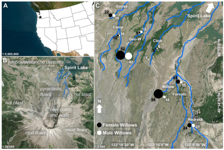
2.1. Site Description

Mount St. Helens erupted in 1980 in a massive lateral blast that transformed over 600 km² of forests, lakes, and streams. A 15-km² area in the main blast zone, called the Pumice Plain, was first buried by over 100 m of sterile pumice, ash, and sand in a 2.8 km³ debris avalanche [90]. It was then hit with a hot lateral blast of flying rock debris, covered in 0.3 km³ of lava, which was as much as 40 m thick in places, and subjected to ash and tephra fall [91]. In the years following the 1980 eruption, springs, seeps, and run-off from snowmelt across the Pumice Plain created five new watersheds (Figure 1), which are slowly seeing the establishment of riparian vegetation. Dominant riparian species include green alder (Alnus viridis) and Sitka willow (Salix sitchensis; hereafter simply willow), the latter of which has been regularly attacked by a stem-boring weevil (Cryptorhynchus lapathi, Curculionidae, Coleoptera) since its introduction in 1989 [83].

2.2. Field Data Collection

Between May–June of 2018, we haphazardly tagged 348 individual and relatively isolated willows across the Pumice Plain and identified each as either male or female based on the presence of reproductive structures [94]. Individual shrubs (a common life history variant of Sitka willow trees based on youth or resource limitation) were tagged with unique identification numbers and colored beads to represent sex, and their locations were recorded by GPS. We also recorded the identity of the nearest stream (Camp, Clear, Forsyth, Geo-West (Geo-W), Goose, Redrock, and Willow Creeks). In the summer of 2019 (26 June to 11 July), we surveyed all willows once for a suite of willow-dependent organisms. These species are varied in their life histories and plant-usage strategies, yet all leave identifiable markings on their willow hosts. Thus, the resulting data, despite a potential temporal mismatch of sampling and organism presence, are not skewed as these markings were maintained by willows at the time of sampling. We surveyed for the presence of attack by the stem-boring poplar weevil, Cryptorhynchus lapathi, based on evidence of frass at the base of stems, dead branches, and/or the presence of adult weevils. We surveyed for the presence of western tent caterpillars, Malacosoma fragilis (Lasiocampidae, Lepidoptera), through evidence of webs, caterpillars, and/or cocoons. We surveyed for evidence of the Pacific willow leaf beetle, Pyrrhalta decora carbo (Chrysomelidae, Coleoptera), based on the presence of skeletonized leaves or larvae. We noted other types of leaf chewing (chewed edges) caused by generalist herbivores, as well as the presence of ants, aphids, and other unidentified caterpillars. We surveyed for the presence of the willow leaf gall sawfly, Pontania pacifica (Tenthredinidae, Hymenoptera), based on the presence of round, red galls. We also noted the presence of a second type of gall, most likely mites of the Eriophyidae family, that presented a range of colors (red, orange, and yellow) on the top surface of the leaf with white spindle-like growths on the underside. We noted the presence of Melampsora spp. rust (an orange fungus common on members of the Salicaceae family), and unidentified endophytes based on the presence of discrete black stromata. Species richness for each tagged willow was determined based on their unique dependent community.

2.3. Leaf Litter Chemistry

Leaf litter was collected from a random subset of the tagged willows (n = 36) from across the Pumice Plain to support related leaf litter decomposition studies. Weevil-induced male and female willow litter was collected in July 2019, as damage due to weevils was more obvious during the growing season, and naturally abscised male and female willow litter was collected in August 2019 [86]. All litter was stored in individual paper sacks and air-dried in the laboratory. Subsamples (0.50 g) were freeze-dried (Millrock Technology, Kingston, NY), ground to a homogeneous consistency (KRUPS Type F203), and used to measure a variety of litter chemical traits (condensed tannins, carbon [C], nitrogen [N], and C:N). First, subsamples of ground material (25 mg) were extracted for soluble condensed tannins with 70% acetone and 10 mM ascorbic acid. We used the butanol–HCl method to determine soluble condensed tannin concentrations [95], with standards purified from local S. sitchensis [96]. Condensed tannin concentrations were determined by measuring absorbance at 550 nm on a spectrophotometer (Spectramax 384, Molecular Devices, San Jose, CA, USA) and comparing samples to a standard curve before being converted to % condensed tannins (%CT). Second, ground subsamples (2 mg) were weighed into tin capsules (5 × 8 mm) to determine %C and %N on an elemental analyzer (2400 CHNS/O Series II System, Perkin Elmer, Waltham, MA, USA). The molar element ratio of C:N was calculated as the ratio of %C divided by the atomic mass of C over %N divided by the atomic mass of N.

2.4. Leaf Area Measurements

Leaf area can influence associated insect and microbial community members [97,98]; thus, fresh leaves were collected from a subset of the tagged willows (n = 122). Roughly five to ten leaves (depending on size) were collected from each willow and either preserved in silica gel or laid onto individual paper sheets in a plant press. Both sample types were dried for several months, weighed to the nearest mg, then scanned on a flatbed scanner. Images were converted to black and white, and leaf area was calculated in ImageJ [99] using a batch process. Specific leaf area (SLA) was calculated by dividing the total leaf area by the mass of the leaves, then by the number of leaves in each sample.

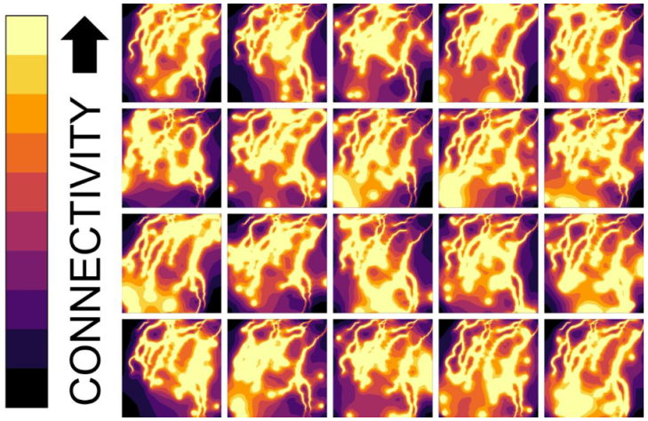
2.5. Landscape Connectivity

Landscape connectivity often determines plant arrangements on a landscape as well as dependent communities [23,61]. Thus, we used the Circuitscape connectivity package in Julia [56] with a high-performance computing cluster to generate continuous landscape connectivity measures for the Pumice Plain based on resistance maps produced in ArcGIS Pro (version 3.0.0) [93]. Primary stream channels were mapped in-field using GPS. Updated and ground-truthed geospatial data was required due to the dynamic nature of our study streams. In this analysis, the greater distance from stream features resulted in greater resistance on the landscape, given that water availability is often the most important limiting factor in post-disturbance community regeneration in the western US [37,38,39,40]. We tested a combination of stream locations and physical parameters such as slope and elevation to predict landscape resistance [100], but landscape resistance changed little compared to only using stream locations. Given similar performance with more complex models, we used the simplest resistance maps created by linearly extrapolating resistance from mapped stream locations to aid in understanding landscape connectivity for the Pumice Plain. Circuitscape runs were based on randomized node locations that produced pairwise electrical current walks through our resistance maps rather than simply producing instantaneous connectivity for known individuals (n = 20 to reduce the computing time and capture within-run variability). We then recreated the Circuitscape output with 20 randomized node repetitions to ensure that sufficient variation based on different arrangements of focal nodes was captured. From each model output, we sampled electrical current for all of our tagged willows as a proxy for an organism’s ability to move through the landscape, thus producing a mean and variance of connectivity at each location.

2.6. Statistical Analyses

All statistical analyses were performed in R version 4.2.0 [101]. We specified three suites of predictor parameters for use in different analytical methods, which test our hypotheses individually based on varying sample sizes. Willow sex was included in all 3 suites, given its influence on ecological communities at each scale and potential interactions with other parameters. The first suite contained the following landscape-level parameters: stream identity, landscape connectivity, and willow sex (n = 335). Stream identity served as both a measure of unique hydrological inputs as well as a proxy for the relative geographical location, given that willow shrubs sampled in this study were growing within 15 m of streams. The second suite contained leaf litter chemistry variables: %C, %N, the C:N molar ratio, %CT, willow sex, and weevil-induction (n = 31). The third and final suite contained SLA and willow sex (n = 109). We then used each of these parameter suites in generalized linear models (GLMs) versus willow community species richness to address our first hypothesis (‘gls’ function in the ‘nlme’ package) [102] and in permutational MANOVAs (PERMANOVAs) versus willow community dissimilarity to address our second hypothesis (999 permutations, ‘adonis2’ function in the ‘vegan’ package) [103]. Community dissimilarities for our PERMANOVAs were determined using the Bray-Curtis dissimilarity index for the leaf-dependent communities found on each tagged willow [104]. To determine the GLMs and PERMANOVAs with the greatest predictive power, we performed Akaike’s Information Criterion (AIC) model selection for all parameter suites [105]. In this method, model parameters were reduced from the full suite of parameters and their most likely interactions to the simplest two-term models to maximize simplicity and ensure effects were adequately captured. We did not consider models with only one term, given that these tests produced similar results to other simple models with added individual terms but no interactions. We also investigated different combinations of parameters with both interactive and non-interactive terms, and the final models we present illustrate a tradeoff between overfitting and an explanation of variance. The AICs of each combination of parameters for each parameter suite were then ranked, and the best overall GLMs and PERMANOVAs were selected.

We analyzed pairwise posthoc stream comparisons for our species richness GLMs using estimated marginal means (‘emmeans’ function in the ‘emmeans’ package) [106] and Tukey’s HSD letters (‘cld’ function in the ‘lsmeans’ package) [107]. We performed NMDS analyses (‘metaMDS’ function in the ‘vegan’ package) [103] to understand community dissimilarity in the parameter space for differences observed in our PERMANOVAs (stress < 0.1, 999 iterations, and 200 random starts). We then used a pairwise PERMANOVA for stream differences based on landscape community dissimilarities (‘pairwise.adonis2’ function in the ‘pairwiseAdonis’ package) [108] and similarity percentage (SIMPER) analyses to understand which community members contributed the most to differences found between streams as well as between male and female willows (‘simper’ function in the ‘vegan’ package) [103]. Using the results of our SIMPER analyses, we generated a heatmap to highlight the most important community members that drove observed differences (‘heatmap’ function in base R).

3. Results

The below are descriptive statistics and visual comparisons intended to provide an illustration of the overarching data structure used in subsequent statistical analyses and are provided in full in Table S1. All of these data are presented in the format of mean ± 1 sd. Overall taxa richness for willow-associated organisms (willow communities) ranged from 1 to 7, with a slightly higher average of 3.27 ± 0.08 taxa on female willows and 3.08 ± 0.09 taxa on male willows. Additionally, taxa richness was highest on willows growing near Forsyth Creek, followed by Camp, Clear, Willow, and Goose, respectively, with the lowest taxa richness on willows growing near Redrock and Geo-W. A mosaic of outputs for all randomized Circuitscape runs can be found in Figure 2. Connectivity values ranged from 0.05 to 1.25 across the Pumice Plain, with average values slightly higher for female willows (0.30 ± 0.02) compared to male willows (0.22 ± 0.02). Connectivity was highest for willows sampled near Willow, followed by Clear, Forsyth, and Geo-W, while the lowest connectivity values were found near Camp, Goose, and Redrock Creeks. Litter %C ranged from 44.80 to 48.80, %N ranged from 0.41 to 2.79, the C:N molar ratio ranged from 19.80 to 134.50, %CT ranged from 1.10 to 28.60, and specific leaf area (SLA) ranged from 2.15 to 25.57 mm² mg⁻¹ across the Pumice Plain. Litter %C, %N, %CT, and SLA were similar between willow males and females, while the C:N ratio was slightly higher for male willows (71.69 ± 10.27) compared to female willows (61.91 ± 8.89). Litter %C was highly similar across willows from all streams, while %N was highest for Forsyth and Willow and lowest for Geo-W and Goose. The C:N molar ratio was highest for willows from Geo-W and Goose, both nearly three times higher than Camp, Forsyth, and Willow Creek. Litter %CT was also highest for willows from Geo-W and Goose, moderately low for Willow and Forsyth, and lowest for Camp Creek. Finally, SLA was highest for willows from Goose and moderately high for Geo-W, which were over four times higher than for Willow Creek.

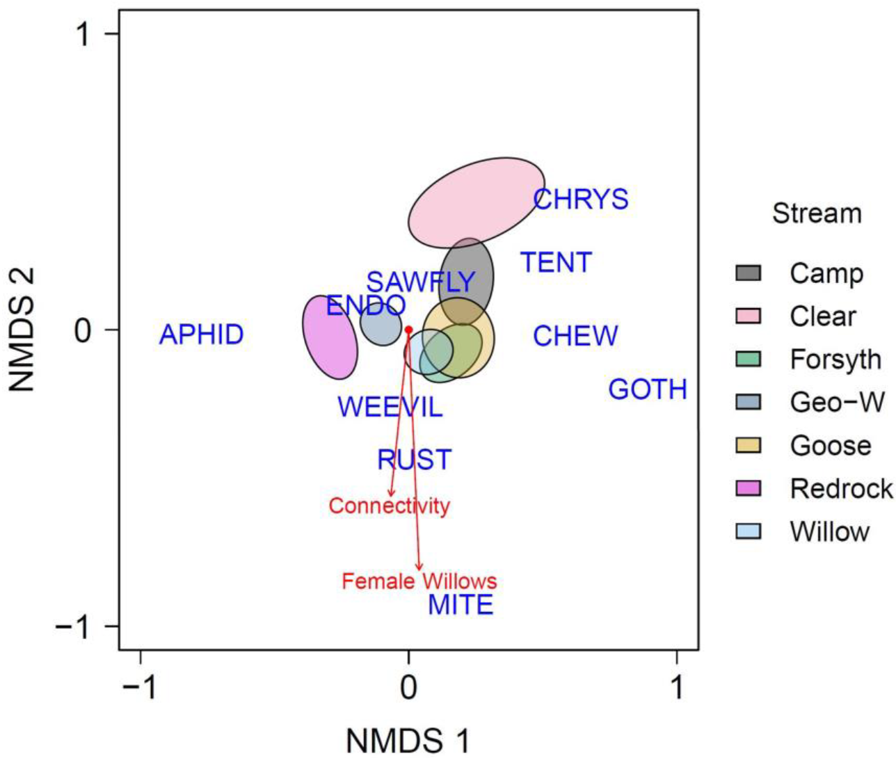
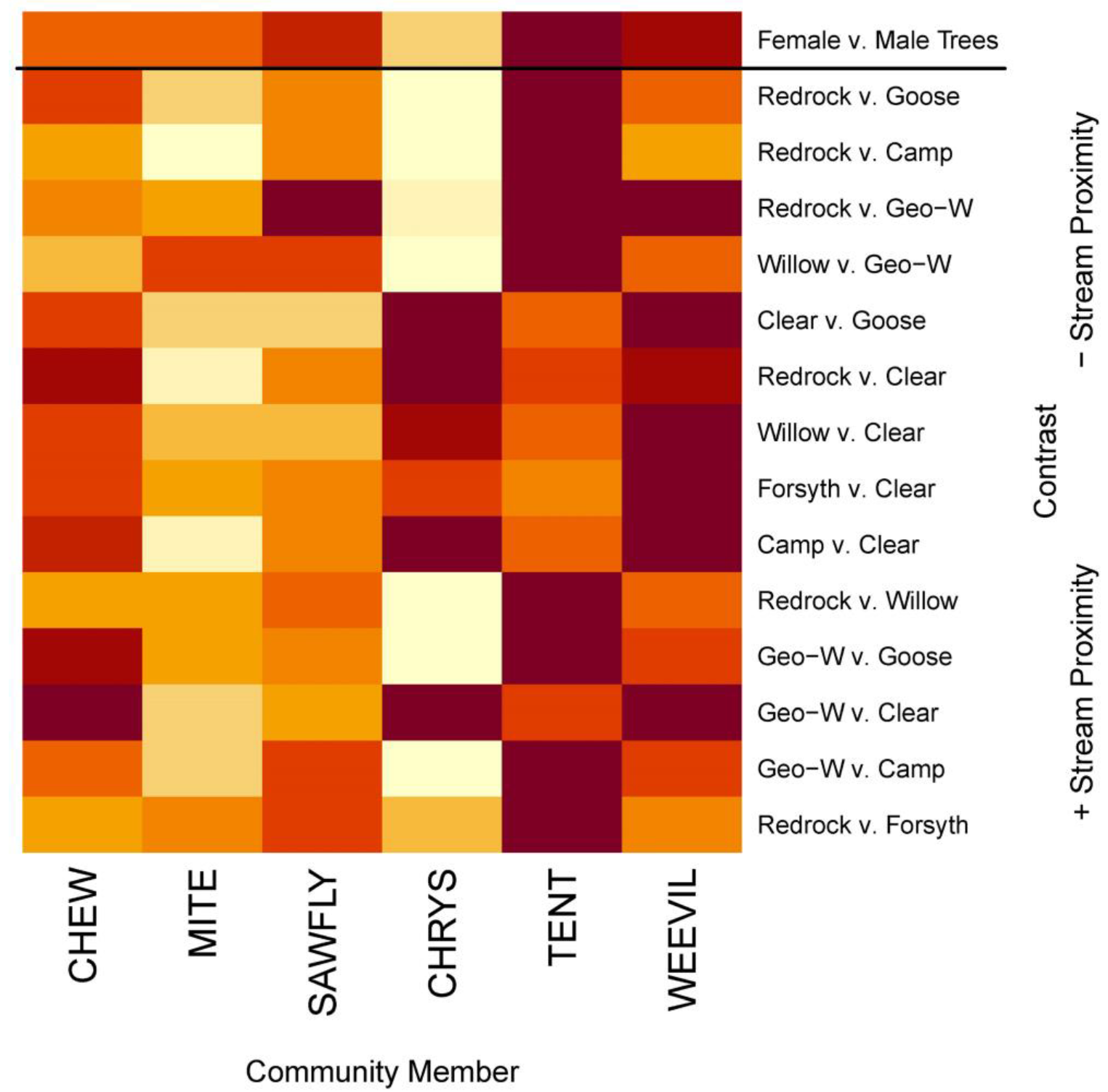
3.1. Landscape-Level Models

We found that landscape connectivity and stream identity with no interaction produced the best landscape-level GLM through model selection (L = −498.826, AIC = 1015.653; Table S2). With this model (

Table 1. Results of three generalized linear models for community richness as a response to changes in landscape, chemistry, and leaf area factors (AIC model selection in Table S2). Factors not present in this table were not part of the best model. Three separate models were used due to differences in the number of observations. The stream factor was categorical and thus tested against its respective first level. A pairwise estimated marginal means analysis can be found for the stream factor in Table S3. Bolded rows indicate significant effects at α = 0.05. Abbreviations: SLA is specific leaf area, df is degrees of freedom, $\widehat{\beta }$ is the effect estimate, σ is the standard error of the effect estimate, t is the test statistic, and p is the null model probability parameter.

Factor	df	$\widehat{\mathit{\beta }}$	σ	t	p
Landscape Model (n = 335)
Connectivity	1	−0.718	0.263	−2.731	0.007
Stream-Clear	1	−0.188	0.394	−0.477	0.633
Stream-Forsyth	1	0.423	0.301	1.406	0.161
Stream-Geo-W	1	−0.808	0.264	−3.059	0.002
Stream-Goose	1	−0.488	0.304	−1.608	0.109
Stream-Redrock	1	−0.936	0.294	−3.187	0.002
Stream-Willow	1	−0.025	0.293	−0.086	0.931
Residuals	327	0.114	1.065	-	-
Litter Chemistry Model (n = 31)
%N	1	1.492	0.657	2.269	0.031
%CT	1	0.150	0.053	2.842	0.008
Weevils	1	0.985	0.996	0.988	0.332
Residuals	28	0.095	0.867	-	-
Leaf Area Model (n = 109)
SLA	1	>−0.001	<0.001	−5.417	<0.001
Willow Sex	1	−0.289	0.186	−1.555	0.123
Residuals	107	0.054	0.969	-	-

), connectivity ($\widehat{\beta }$ = −0.718, σ = 0.263, t₃₂₇ = −2.731, p = 0.007) explained differences in willow community species richness where less connected shrubs were associated with higher species richness. The effects of stream identity were, however, varied given that each stream was only tested, in turn, against the first level of the stream factor (Camp), where only Geo-W ($\widehat{\beta }$ = −0.808, σ = 0.264, t₃₂₇ = −3.059, p = 0.002) and Redrock ($\widehat{\beta }$ = −0.936, σ = 0.294, t₃₂₇ = −3.187, p = 0.002) produced differences in species richness. Thus, from our pairwise posthoc investigation (Table S3), we found three stream groupings for willows in terms of richness that differed from each other: (a) Redrock, Geo-W, Goose, and Clear; (b) Goose, Clear, Willow, and Camp; and (c) Clear, Willow, Camp, and Forsyth. Overlaps of stream identity for these groupings can be considered not different from any other stream in either grouping while the absolute differences between groupings are maintained.

We found that connectivity, stream identity, and willow sex with no interaction produced the best landscape-level PERMANOVA through model selection (L = −909.464, AIC = 1046.270; Table S4). All three parameters predicted differences in community dissimilarity on willow shrubs in the final model (

Table 2. Results of three permutational MANOVA (PERMANOVA) tests for community dissimilarity as a response to changes in the overall landscape, chemistry, and leaf area factors (AIC model selection in Table S4). Factors not present in this table were not part of the best model. Three separate models were used due to differences in the number of observations for each subset of data. Differences found for continuous variables were analyzed using NMDS analyses in Figure 3 and Figure S1. Bolded rows indicate significant effects at α = 0.05. Abbreviations: df is degrees of freedom, SS is the sum of squares, R² is the correlation coefficient, F is a pseudo-F test statistic, and p is the null model probability parameter.

Factor	df	SS	R2	F	p
Landscape Model (n = 335)
Connectivity	1	0.361	0.013	5.298	0.003
Willow Sex	1	0.386	0.014	5.670	0.003
Stream	6	5.600	0.196	13.716	0.001
Residual	326	22.183	0.778	-	-
Litter Chemistry Model (n = 31)
%N	1	0.097	0.056	1.748	0.166
%CT	1	0.080	0.046	1.444	0.237
Residual	28	1.559	0.898	-	-
Leaf Area Model (n = 109)
SLA	1	0.353	0.041	4.575	0.015
Willow Sex	1	0.064	0.007	0.825	0.501
Residual	107	8.179	0.952	-	-

; connectivity: SS = 0.361, F_1,326 = 5.298, p = 0.003; stream identity: SS = 0.386, F_6,326 = 13.716, p = 0.003; and willow sex: SS = 5.600, F_1,326 = 5.670, p = 0.001). Our landscape-level NMDS analysis (Figure 3) revealed that weevils, fungal rust, and galling mites were strongly associated with both female willows and landscape connectivity. On the other hand, we found that sawflies and endophytes were negatively associated with female willows (i.e., associated with males) and landscape connectivity. Chrysomelid beetles and tent caterpillars were weakly negatively associated with female willows and landscape connectivity, while all other community members (aphids, other caterpillars, and other chewers) were not associated with either factor. Our pairwise stream analysis indicated that willow-dependent community compositions for Redrock and Clear were different from all other streams and each other (Table S5). Furthermore, the compositions for Geo-W were different from all other streams, with the exception of Forsyth.

Our SIMPER analysis (Figure 4 and Table S6) revealed that all stream-based differences in the willow communities above were driven in some way by tent caterpillars (15/15 comparisons) and nearly all by weevils (14/15 comparisons; only Redrock v. Camp was not). In general, community differences among streams that were closer together as well as farther away tended to be driven mostly by tent caterpillars, while those at intermediate distances from one another were driven primarily by weevils, chrysomelid beetles, and other chewers. Additionally, sawflies and chewers were important drivers for the majority of observed differences (12/15 and 11/15, respectively) but were not as important as tent caterpillars or weevils overall. Chrysomelid beetles were very important drivers for all differences found between Clear and other streams despite driving differences in fewer than half of the stream comparisons (6/15). The presence of endophytes, rust, aphids, and other caterpillars did not drive any community differences, and the presence of galling mites only drove differences in two comparisons (Redrock vs. Forsyth and Willow vs. Geo-W). Finally, we found that community differences between female and male willows were driven primarily by tent caterpillars and weevils but also, in some manner, by sawflies, mites, and other chewers.

3.2. Leaf Litter Chemistry Models

We found that %N, %CT, and weevil presence with no interaction produced the best leaf litter chemistry GLM through model selection (L = −40.386, AIC = 90.771; Table S2). In this model (Table 1), both %N ($\widehat{\beta }$ = 1.492, σ = 0.657, t₂₈ = 2.269, p = 0.031) and %CT ($\widehat{\beta }$ = 0.150, σ = 0.053, t₂₈ = 2.842, p = 0.008) explained differences in willow-dependent community species richness, where species richness was positively associated with %N and %CT. Weevil presence did not drive differences in species richness ($\widehat{\beta }$ = 0.985, σ = 0.996, t₂₈ = 0.988, p = 0.332). We also found that %N and %CT with no interaction produced the best leaf litter chemistry PERMANOVA through model selection (L = −92.689, AIC = 19.765; Table S4). However, neither %N (SS = 0.097, F_1,28 = 1.748, p = 0.166) nor %CT (SS = 0.080, F_1,28 = 1.444, p = 0.237) explained differences in willow community dissimilarity in the final model (Table 2).

3.3. Leaf Area Models

We found that SLA and willow sex with no interaction produced the best leaf area GLM through model selection (L = −162.167, AIC = 332.333; Table S2). In this model (Table 1), only SLA ($\widehat{\beta }$ = >−0.001, σ = <0.001, t₁₀₇ = −5.417, p = <0.001) explained differences in willow community species richness, where species richness was negatively associated with SLA. Willow sex did not drive differences in species richness in this context ($\widehat{\beta }$ = −0.289, σ = 0.186, t₁₀₇ = −1.555, p = 0.123). We also found that SLA and willow sex with no interaction produced the best leaf area PERMANOVA through model selection (L = −282.286, AIC = 235.071; Table S4). Only SLA (SS = 0.353, F_1,107 = 4.575, p = 0.015) and not willow sex in this model (SS = 0.064, F_1,107 = 0.825, p = 0.501) explained differences found in willow-dependent community dissimilarity (Table 2). Our leaf area NMDS analysis (Figure S1) revealed that only endophytes were positively associated with SLA. Weevils and galling mites were strongly negatively associated with SLA, while fungal rust and chewers were weakly negatively associated. Tent caterpillars, sawflies, and chrysomelid beetles were not associated with SLA.

4. Discussion

Given its relative simplicity, species richness is often a fundamental yet coarse first investigation into how geospatial, structural, or chemical parameters influence ecological communities [109,110]. Contrary to our expectations, landscape connectivity and specific leaf area (SLA) were negatively related to species richness such that less-connected willow shrubs and those with smaller leaves housed more species-rich communities. Landscape connectivity, as well as SLA, typically facilitate the establishment of plant-dependent species given that higher connectivity makes target plants more accessible across the landscape and greater SLA presents as a larger food source. However, our results indicate that connectivity and SLA may have unintended consequences for a species-poor primary successional community. Mechanistically, larger willow leaves could produce a tradeoff with palatability in which certain species may avoid leaves with unfavorable chemical traits [87,88], be that tradeoff created by willow age or sex [82,86]. In addition, larger willow leaves could facilitate competition, which leads to an imbalance of species present or alters microbial establishment, which would further influence leaf palatability [111,112,113]. For connectivity, species that require greater connectivity of willows to establish across a landscape may possess the ability to outcompete others, resulting in the reduced species richness we observe. Furthermore, species that can utilize less-connected willows farther from stream edges may simply avoid over-utilized shrubs with higher connectivity. In conjunction with sex-ratio dynamics, where willows farther from streams are more likely to be male [82], community compositions are likely to be different on willows experiencing different levels of connectivity. We also found that species richness was differentially related to the identity of streams nearest willow samples and that those streams were organized into three separate groupings. Interestingly, species richness appeared to be randomly distributed across the Pumice Plain, as none of the three groupings shared distinct geospatial placements. This potentially indicates that the proximity of streams does not facilitate mutual levels of species richness. For the chemistry of willow leaf litter, we found that %N and %CT positively influenced species richness, while no other parameters explained differences or improved model power. The positive influence of nitrogen is not unexpected as nitrogen is often limiting in many plant-dependent communities, and higher nitrogen often results in more energetically favorable food sources [114,115]. However, tannins are typically astringent and bitter components of plant chemistry, with the unique ability to deter many types of herbivores [70]. Their positive influence on species richness could be the result of a food-limited environment where willow shrubs are often simply the best food source available to the species found on the Pumice Plain. Willow sex and interactions with other parameters did not influence species richness for the leaf area model and did not add to the explanatory power of our landscape and litter chemistry models. This result is contrary to previous findings that female willows typically facilitate species presence, particularly stem-boring weevils [83]. However, for such a species-poor community, the effects of willow sex on richness may not be as prominent as sex effects on community structure.

While species richness can provide a broad-scale view into the assembly of ecological communities, understanding influences on community composition can provide critical deeper insights into the life history and dispersal characteristics that could affect establishment across the landscape [116,117]. Parallel to species richness, we found that landscape connectivity, SLA, and stream identity drove differences in community structures among individual willow shrubs. Furthermore, willow sex predicted community dissimilarity despite no overall influence on species richness. Landscape connectivity was positively associated with weevils, fungal rust, and galling mites, meaning that willows that were more connected experienced higher rates of attack from these community members. These organisms share a common life history based on passive physical dispersal ability in which they utilize more connected habitats to move from host to host. For example, fungal rust is notably spread through spores and potentially spreads more easily in denser shrub communities with higher water availability [118], while galling mites disperse after adult eclosure through ballooning into the air and passively transferring to nearby plants [119,120]. Weevil adults seldom fly and often lay eggs on the same individual from which they emerged as larvae [83]. Directional flyers, which exhibit the ability to disperse actively across the Pumice Plain and select hosts [121], such as tent caterpillars and chrysomelid beetles, were less associated with landscape connectivity alongside aphids, which have been noted to travel large distances along the ground in search of living plant material [122]. Thus, our findings indicate that passive host use is directly related to increased landscape connectivity, while the ability to actively select hosts mitigates the necessity of more connected habitats. We also observed that endophytes were negatively related to connectivity, which is contrary to expectations of low dispersal ability for symbiotic microbes. Upon further investigation, however, endophytes were present on nearly every willow, and their ubiquitous life history in communities of the Pumice Plain is a finding mirrored in other studies [123]. Results for willow sex were similar to the above results for landscape connectivity, where female willows were associated with the same species as increased landscape connectivity. These results indicate that certain willow-dependent organisms differentially utilize willow shrubs of different sexes, meaning that the placement of willow sexes on the landscape can be a fundamental predictor of dependent community assembly. However, we found no association between leaf chemistry and community dissimilarity, suggesting that the influence of willow sex is more complex than potential differences in leaf chemistry. We also predicted that endophytic symbionts would prefer female willows, yet their ubiquity on all willows indicates that there may be no mechanism for endophytes to preferentially utilize females. We did not explicitly test the landscape connectivity of female versus male willows, but our results suggest that female willows were associated with higher overall connectivity. However, it is important to note that we did not sample all willow individuals across the Pumice Plain and that this distinction could simply be caused by the locations where certain willows were sampled (i.e., distances from the nearest stream).

Landscape connectivity is a broad-scale metric of habitat structure that is essential in understanding how certain organisms can disperse between habitat locations [124], but it is also important to understand how nested levels of habitat structure can assemble communities and predict dissimilarity. Stream identity represents habitat structure at a finer scale than connectivity as a proxy for physical landscape location and allows us to investigate how stream heterogeneity influences community identity. Stream identity also allowed us to test geographic location in a clearer way than with 2-dimensional geographic coordinates, given that individual sampling coordinates for willows near different streams overlapped and that differences in willow-dependent communities should be more associated with proximity to the same stream (given proximity and connectivity to each other) than with absolute coordinate locations. Furthermore, a single categorical value for each willow location was critical for testing our hypotheses with a suite of assembly characteristics (landscape, chemistry, and leaf area) rather than with more complex pairwise distances across the Pumice Plain. Overall, we observed differences in 14/21 comparisons of willow-dependent community dissimilarity between varying stream locations. These differences were driven mostly by comparisons of other streams to Redrock, Clear, and Geo-W, as well as comparisons to each other. These streams are spread across the Pumice Plain and are not part of an interconnected network like Forsyth, Redrock, and Willow; thus, the relative geographic location appears not to influence dependent community assembly. However, willows from each stream alone harbored unique subsets of the overall dependent community (e.g., Redrock willows with aphids, Clear with chrysomelid beetles, Camp with sawflies, etc.), suggesting that specific locations of willows near individual streams (i.e., independent geographic locations) do drive community assembly. We found that the presence of tent caterpillars and weevils drove the majority of comparisons, where weevils were more important in stream comparisons of moderate distance and tent caterpillars were more important in all others. Thus, tent caterpillars may avoid connected willows that have more weevils since the outer comparisons in both directions of our heat map are between streams with higher landscape connectivity overall. Tent caterpillars may also not expend energy in finding connected willows given their lack of mobility constraints, or they may simply avoid willow branches attacked by weevils, as those branches are more likely to die and collapse. These findings expand on our previous species richness results as the absences of other community members, such as chrysomelid beetles and chewing guild herbivores, also drive comparisons in which weevils are dominant, meaning that these community members are disassociated with the presence of weevils. In a species-poor community such as this, the lack of certain community members can have a powerful effect on the services and resilience of the resulting ecosystem [125,126,127,128]. Leaf area is a much finer metric of habitat structure, given its role in potential food availability, but it can also be important in a willow’s ability to house different types of species. We found that SLA was not positively associated with any community member, while it was negatively associated with several organisms, such as weevils, galling mites, and rust. This finding provides a potential mechanism for lower species richness associated with higher SLA, in that the presence of no one organism led to a lower presence of others on larger leaves. Rather, all community members either preferred smaller leaves or indifferently utilized willows regardless of leaf size, indicating that some composition (e.g., energy density or secondary chemicals) within larger leaves was less preferable than smaller leaves [129,130]. As a habitat metric, this finding has important implications for landscape management as leaf size can be a proxy for leaf health and thus habitat carrying capacity [131,132], and targeting certain habitat structures (e.g., willow ages or sexes) in this population can facilitate willow-dependent community establishment.

Our findings indicate that community assembly on the Pumice Plain may be directed by a variety of different factors. However, the scales at which each of these factors produced an effect were markedly different. For example, we deliberately tested willow sex within each suite of model parameters to understand parameter interactions (landscape, chemical, and leaf area) but found that willow sex variably contributed to model explanatory power and only produced differences for richness via the leaf area dataset and community structure via the landscape-level model. This finding implies that scale of effect, in which a parameter may produce an effect at one scale but not at others, could be a crucial consideration for the analysis of metacommunity dynamics across the Pumice Plain and is a possible avenue for future research [133]. Additionally, all chemistry and leaf area parameters were performed for smaller subsets of the overall data due to sampling limitations. Considering the varied effect of willow sex, it is possible that an expanded set of data, or even for the full set of surveyed willows for this research, could elucidate heterogeneous patterns of community response to different factors. Despite this, we have illustrated that the metacommunity across willows on the Pumice Plain is regenerating based on this array of community-structuring parameters. Specifically, we found that willows distinct by different stream locations, leaf area, leaf chemistry, sex, and connectivity at the landscape-scale are habitats for different subsets of the full community. This heterogeneity of use by different community members is essential for facilitating metacommunity interactions among different species [10,134], promoting ecosystem resilience [135], and establishing a diversity of ecosystem services [136]. Thus, our findings are critical for understanding community regeneration as a function of primary succession following a major disturbance that effectively reset landscape processes and dynamics. Furthermore, our work is important to direct future research focused over longer periods of time to understand the true trajectory of metacommunity regeneration, given this study was conducted at one point in time. This is especially important when considering the dynamics of newly developing streams, of which our target streams are, in that different streams may be present year-in and year-out [137]. The establishment of new willows on the landscape could be highly dependent on the seasonal availability of water [138,139], and landscape connectivity will be dependent on future stream locations and their variability. Furthermore, landscape connectivity for currently established willows, such as those sampled for this study, will change based on shifting hydrodynamics. Thus, mapping the same suites of parameters over time will allow us to understand how the community changes over time based on these parameters and how the landscape may change in the future.

Landscape connectivity and habitat structure, in association with dispersal ability, often dictate how organisms will spread throughout a landscape [23,24]. However, effectively capturing a measure of landscape connectivity and, thus, dispersal potential for organisms requiring high connectivity is difficult. In this study, we utilize circuit theory in Circuitscape, a modeling method that measures landscape connectivity not simply based on the absolute distribution of a species but as a process of varying resistance inherent to the landscape itself. The majority of other studies utilizing circuit theory analyze the connectivity between specific individuals of the same species [58,59], while we treat the connectivity produced as a community assembly process independent of willow sampling locations (i.e., using randomized starts). In this manner, we tested hypotheses of community assembly versus potential landscape connectivity and were able to make judgments about what level of connectivity was influential for specific community members. Classic measures of landscape connectivity simply do not capture these dynamics as they typically produce one output for a given pairwise comparison rather than a range of data and a testable central tendency [47,48,49,53]. In our method, we effectively simulated how an organism might experience the landscape: randomness and variance are much more important given that migrants rarely enter or disperse from the same places, especially for a primary successional landscape. To our knowledge, this application of circuit theory is novel and could present new opportunities for other habitats experiencing rapid change or those which are critically understudied, given that the production of resistance maps could be readily achieved with adequate remote-sensing data.

5. Conclusions

Landscape connectivity can be a powerful tool for the management of primary successional landscapes; in our study, we found that variations in landscape connectivity can sustain variations in organismal life histories such that patchy mosaics of connectivity can support a wider range of potential community members. Furthermore, simply targeting more connected landscapes has the potential to facilitate the expansion of invasive species. If maintenance and further regeneration of metacommunity dynamics is a target for restoration and management, understanding the potential pathways of invasibility is vital given the influences that species like the stem-boring poplar weevil can have on the communities to which they are introduced [84,85,86]. Studies in ecology often experience difficulty in extrapolating results from areas too fine-scaled to larger landscapes but also with broader parameters such as physical location applied to more fine-scale processes. We successfully capture dynamics across three separate resolutions of community structure: leaf area, physical location via nearest streams, and overall landscape connectivity. Utilizing these dynamics, in conjunction with the maintenance of heterogeneity in community-structuring parameters (e.g., physical and chemical factors), will be key in facilitating further development and regeneration of willow-dependent communities across the Pumice Plain.

References

1. Gaynor, K.M.; Hojnowski, C.E.; Carter, N.H.; Brashares, J.S. The influence of human disturbance on wildlife nocturnality. Science 2018, 360, 1232–1235. [Google Scholar] [CrossRef] [PubMed]
2. Laurance, W.F.; Useche, D.C.; Rendeiro, J.; Kalka, M.; Bradshaw, C.J.A.; Sloan, S.P.; Laurance, S.G.; Campbell, M.; Abernethy, K.; Alvarez, P.; et al. Averting biodiversity collapse in tropical forest protected areas. Nature 2012, 489, 290–294. [Google Scholar] [CrossRef] [PubMed]
3. Lindenmayer, D.B.; Likens, G.E.; Franklin, J.F. Rapid responses to facilitate ecological discoveries from major disturbances. Front. Ecol. Environ. 2010, 8, 527–532. [Google Scholar] [CrossRef]
4. Morcillo, D.O.; Steiner, U.K.; Grayson, K.L.; Ruiz-Lambides, A.V.; Hernández-Pacheco, R. Hurricane-induced demographic changes in a non-human primate population. R. Soc. Open Sci. 2020, 7, 200173. [Google Scholar] [CrossRef]
5. Major, J.J.; Pierson, T.C.; Dinehart, R.L.; Costa, J.E. Sediment yield following severe volcanic disturbance—A two-decade perspective from Mount St. Helens. Geology 2000, 28, 819–822. [Google Scholar] [CrossRef]
6. Zobel, D.B.; Antos, J.A.; Fischer, D.G. Secondary disturbance following a deposit of volcanic tephra: A 30-year record from old-growth forest understory. Can. J. For. Res. 2021, 51, 1541–1549. [Google Scholar] [CrossRef]
7. Jentsch, A.; White, P. A theory of pulse dynamics and disturbance in ecology. Ecology 2019, 100, e02734. [Google Scholar] [CrossRef]
8. Shackelford, N.; Starzomski, B.M.; Banning, N.C.; Battaglia, L.L.; Becker, A.; Bellingham, P.J.; Bestelmeyer, B.; Catford, J.A.; Dwyer, J.M.; Dynesius, M.; et al. Isolation predicts compositional change after discrete disturbances in a global meta-study. Ecography 2017, 40, 1256–1266. [Google Scholar] [CrossRef]
9. Banks, S.C.; Cary, G.J.; Smith, A.L.; Davies, I.D.; Driscoll, D.A.; Gill, A.M.; Lindenmayer, D.B.; Peakall, R. How does ecological disturbance influence genetic diversity? Trends Ecol. Evol. 2013, 28, 670–679. [Google Scholar] [CrossRef]
10. Holyoak, M.; Caspi, T.; Redosh, L.W. Integrating disturbance, seasonality, multi-year temporal dynamics, and dormancy into the dynamics and conservation of metacommunities. Front. Ecol. Evol. 2020, 8, 571130. [Google Scholar] [CrossRef]
11. Urban, M.C. Disturbance heterogeneity determines freshwater metacommunity structure. Ecology 2004, 85, 2971–2978. [Google Scholar] [CrossRef]
12. Vass, M.; Langenheder, S. The legacy of the past: Effects of historical processes on microbial metacommunities. Aquat. Microb. Ecol. 2017, 79, 13–19. [Google Scholar] [CrossRef]
13. Rohal, C.B.; Cranney, C.; Kettenring, K.M. Abiotic and landscape factors constrain restoration outcomes across spatial scales of a widespread invasive plant. Front. Plant Sci. 2019, 10, 481. [Google Scholar] [CrossRef]
14. Sharp, S.J.; Angelini, C. The role of landscape composition and disturbance type in mediating salt marsh resilience to feral hog invasion. Biol. Invasions 2019, 21, 2857–2869. [Google Scholar] [CrossRef]
15. Biswas, S.R.; Mallik, A.U.; Braithwaite, N.T.; Biswas, P.L. Effects of disturbance type and microhabitat on species and functional diversity relationship in stream-bank plant communities. For. Ecol. Manag. 2019, 432, 812–822. [Google Scholar] [CrossRef]
16. Newman, E.A. Disturbance ecology in the anthropocene. Front. Ecol. Evol. 2019, 7, 147. [Google Scholar] [CrossRef]
17. Rodewald, A.D.; Yahner, R.H. Influence of landscape composition on avian community structure and associated mechanisms. Ecology 2001, 82, 3493–3504. [Google Scholar] [CrossRef]
18. Barba-Escoto, L.; Ponce-Mendoza, A.; García-Romero, A.; Calvillo-Medina, R.P. Plant community strategies responses to recent eruptions of Popocatépetl volcano, Mexico. J. Veg. Sci. 2019, 30, 375–385. [Google Scholar] [CrossRef]
19. Shackelford, N.; Standish, R.J.; Lindo, Z.; Starzomski, B.M. The role of landscape connectivity in resistance, resilience, and recovery of multi-trophic microarthropod communities. Ecology 2018, 99, 1164–1172. [Google Scholar] [CrossRef]
20. Sferra, C.O.; Hart, J.L.; Howeth, J.G. Habitat age influences metacommunity assembly and species richness in successional pond ecosystems. Ecosphere 2017, 8, e01871. [Google Scholar] [CrossRef]
21. Montoya, D. Challenges and directions toward a general theory of ecological recovery dynamics: A metacommunity perspective. One Earth 2021, 4, 1083–1094. [Google Scholar] [CrossRef]
22. Vanschoenwinkel, B.; Buschke, F.; Brendonck, L. Disturbance regime alters the impact of dispersal on alpha and beta diversity in a natural metacommunity. Ecology 2013, 94, 2547–2557. [Google Scholar] [CrossRef]
23. Uroy, L.; Ernoult, A.; Mony, C. Effect of landscape connectivity on plant communities: A review of response patterns. Landsc. Ecol. 2019, 34, 203–225. [Google Scholar] [CrossRef]
24. Zeller, K.A.; Lewison, R.; Fletcher, R.J.; Tulbure, M.G.; Jennings, M.K. Understanding the importance of dynamic landscape connectivity. Land 2020, 9, 303. [Google Scholar] [CrossRef]
25. Fahrig, L.; Paloheimo, J. Effect of spatial arrangement of habitat patches on local population size. Ecology 1988, 69, 468–475. [Google Scholar] [CrossRef]
26. Mony, C.; Vannier, N.; Brunellière, P.; Biget, M.; Coudouel, S.; Vandenkoornhuyse, P. The influence of host-plant connectivity on fungal assemblages in the root microbiota of Brachypodium pinnatum. Ecology 2020, 101, e02976. [Google Scholar] [CrossRef]
27. Rotchés-Ribalta, R.; Winsa, M.; Roberts, S.P.M.; Öckinger, E. Associations between plant and pollinator communities under grassland restoration respond mainly to landscape connectivity. J. Appl. Ecol. 2018, 55, 2822–2833. [Google Scholar] [CrossRef]
28. Brudvig, L.A.; Damaschen, E.I.; Tewksbury, J.J.; Haddad, N.M.; Levey, D.J. Landscape connectivity promotes plant biodiversity spillover into non-target habitats. Proc. Natl. Acad. Sci. USA 2009, 106, 9328–9332. [Google Scholar] [CrossRef]
29. Joern, A.; Laws, A.N. Ecological mechanisms underlying arthropod species diversity in grasslands. Annu. Rev. Entomol. 2013, 58, 19–36. [Google Scholar] [CrossRef]
30. Laurance, W.F. Theory meets reality: How habitat fragmentation research has transcended island biogeographic theory. Biol. Conserv. 2008, 141, 1731–1744. [Google Scholar] [CrossRef]
31. Allen, C.; Gonzales, R.; Parrott, L. Modelling the contribution of ephemeral wetlands to landscape connectivity. Ecol. Model. 2020, 419, 108944. [Google Scholar] [CrossRef]
32. Bishop-Taylor, R.; Tulbure, M.G.; Broich, M. Surface-water dynamics and land use influence landscape connectivity across a major dryland region. Ecol. Appl. 2017, 27, 1124–1137. [Google Scholar] [CrossRef] [PubMed]
33. Bishop-Taylor, R.; Tulbure, M.G.; Broich, M. Impact of hydroclimatic variability on regional-scale landscape connectivity across a dynamic dryland region. Ecol. Indic. 2018, 94, 142–150. [Google Scholar] [CrossRef]
34. Mathys, A.; Coops, N.C.; Waring, R.H. Soil water availability effects on the distribution of 20 tree species in western North America. For. Ecol. Manag. 2014, 313, 144–152. [Google Scholar] [CrossRef]
35. Andrus, R.A.; Harvey, B.J.; Rodman, K.C.; Hart, S.J.; Veblen, T.T. Moisture availability limits subalpine tree establishment. Ecology 2018, 99, 567–575. [Google Scholar] [CrossRef]
36. López, B.C.; Holmgren, M.; Sabaté, S.; Gracia, C.A. Estimating annual rainfall threshold for establishment of tree species in water-limited ecosystems using tree-ring data. J. Arid Environ. 2008, 72, 602–611. [Google Scholar] [CrossRef]
37. Del Arroyo, O.G.; Silver, W.L. Disentangling the long-term effects of disturbance on soil biogeochemistry in a wet tropical forest ecosystem. Glob. Change Biol. 2018, 24, 1673–1684. [Google Scholar] [CrossRef]
38. Kemp, K.B.; Higuera, P.E.; Morgan, P.; Abatzoglou, J.T. Climate will increasingly determine post-fire tree regeneration success in low-elevation forests, Northern Rockies, USA. Ecosphere 2019, 10, e02568. [Google Scholar] [CrossRef]
39. Romero, L.M.; Smith III, T.J.; Fourqurean, J.W. Changes in mass and nutrient content of wood during decomposition in a south Florida mangrove forest. J. Ecol. 2005, 93, 618–631. [Google Scholar] [CrossRef]
40. Stevens-Rumann, C.S.; Morgan, P. Tree regeneration following wildfires in the western US: A review. Fire Ecol. 2019, 15, 15. [Google Scholar] [CrossRef]
41. Ciccazzo, S.; Esposito, A.; Borruso, L.; Brusetti, L. Microbial communities and primary succession in high altitude mountain environments. Ann. Microbiol. 2016, 66, 43–60. [Google Scholar] [CrossRef]
42. Na, X.; Yu, H.; Wang, P.; Zhu, W.; Niu, Y.; Huang, J. Vegetation biomass and soil moisture coregulate bacterial community succession under altered precipitation regimes in a desert steppe in northwestern China. Soil Biol. Biochem. 2019, 136, 107520. [Google Scholar] [CrossRef]
43. Walker, L.R.; Chapin, F.S. Physiological controls over seedling growth in primary succession on an Alaskan floodplain. Ecology 1986, 67, 1508–1523. [Google Scholar] [CrossRef]
44. Yurkewycz, R.P.; Bishop, J.G.; Crisafulli, C.M.; Harrison, J.A.; Gill, R.A. Gopher mounds decrease nutrient cycling rates and increase adjacent vegetation in volcanic primary succession. Oceologia 2014, 176, 1135–1150. [Google Scholar] [CrossRef] [PubMed]
45. Mony, C.; Uroy, L.; Khalfallah, F.; Haddad, N.; Vandenkoornhuyse, P. Landscape connectivity for the invisibles. Ecography 2022, 2022, e06041. [Google Scholar] [CrossRef]
46. Wang, B.; Tian, C.; Sun, J. Effects of landscape complexity and stand factors on arthropod communities in poplar forests. Ecol. Evol. 2019, 9, 7143–7156. [Google Scholar] [CrossRef]
47. Frazier, A.E.; Kedron, P. Landscape metrics: Past progress and future directions. Curr. Landsc. Ecol. Rep. 2017, 2, 63–72. [Google Scholar] [CrossRef]
48. McRae, B.H.; Dickson, B.G.; Keitt, T.H.; Shah, V.B. Using circuit theory to model connectivity in ecology, evolution, and conservation. Ecology 2008, 89, 2712–2724. [Google Scholar] [CrossRef]
49. Minor, E.S.; Urban, D.L. A graph-theory framework for evaluating landscape connectivity and conservation planning. Conserv. Biol. 2008, 22, 297–307. [Google Scholar] [CrossRef]
50. Baguette, M.; Dyck, H.V. Landscape connectivity and animal behavior: Functional grain as a key determinant for dispersal. Landsc. Ecol. 2007, 22, 1117–1129. [Google Scholar] [CrossRef]
51. Diniz, M.F.; Cushman, S.A.; Machado, R.B.; Júnior, P.D.M. Landscape connectivity modeling from the perspective of animal dispersal. Landsc. Ecol. 2020, 35, 41–58. [Google Scholar] [CrossRef]
52. Tischendorf, L.; Fahrig, L. On the usage and measurement of landscape connectivity. Oikos 2003, 90, 7–19. [Google Scholar] [CrossRef]
53. McRae, B.H.; Beier, P. Circuit theory predicts gene flow in plant and animal populations. Proc. Natl. Acad. Sci. USA 2007, 104, 19885–19890. [Google Scholar] [CrossRef]
54. McRae, B.H.; Hall, S.A.; Beier, P.; Theobald, D.M. Where to restore ecological connectivity? Detecting barriers and quantifying restoration benefits. PLoS ONE 2012, 7, e52604. [Google Scholar] [CrossRef]
55. Laliberté, J.; St-Laurent, M.-H. Validation of functional connectivity modeling: The Achilles’ heel of landscape connectivity mapping. Landsc. Urban Plan. 2020, 202, 103878. [Google Scholar] [CrossRef]
56. Hall, K.R.; Anantharaman, R.; Landau, V.A.; Clark, M.; Dickson, B.G.; Jones, A.; Platt, J.; Edelman, A.; Shah, V.B. Circuitscape in Julia: Empowering dynamic approaches to connectivity assessment. Land 2021, 10, 301. [Google Scholar] [CrossRef]
57. Zeller, K.A.; Wattles, D.W.; Destefano, S. Evaluating methods for identifying large mammal road crossing locations: Black bears as a case study. Landsc. Ecol. 2020, 35, 1799–1808. [Google Scholar] [CrossRef]
58. Koen, E.L.; Bowman, J.; Garroway, C.J.; Mills, S.C.; Wilson, P.J. Landscape resistance and American marten gene flow. Landsc. Ecol. 2012, 27, 29–43. [Google Scholar] [CrossRef]
59. Lozier, J.D.; Strange, J.P.; Koch, J.B. Landscape heterogeneity predicts gene flow in a widespread polymorphic bumble bee, Bombus bifarius (Hymenoptera: Apidae). Conserv. Genet. 2013, 14, 1099–1110. [Google Scholar] [CrossRef]
60. Sackett, L.C.; Cross, T.B.; Jones, R.T.; Johnson, W.C.; Ballare, K.; Ray, C.; Collinge, S.K.; Martin, A.P. Connectivity of prairie dog colonies in an altered landscape: Inferences from analysis of microsatellite DNA variation. Conserv. Genet. 2012, 13, 407–418. [Google Scholar] [CrossRef]
61. Dickson, B.G.; Albano, C.M.; Anantharaman, R.; Beier, P.; Fargione, J.; Graves, T.A.; Gray, M.E.; Hall, K.R.; Lawler, J.J.; Leonard, P.B.; et al. Circuit-theory applications to connectivity science and conservation. Conserv. Biol. 2018, 33, 239–249. [Google Scholar] [CrossRef] [PubMed]
62. Naiman, R.J.; Bechtold, J.S.; Drake, D.C.; Latterell, J.J.; O’Keefe, T.C.; Balian, E.V. Origins, patterns, and importance of heterogeneity in riparian systems. In Ecosystem Function in Heterogeneous Landscapes; Lovett, G.M., Turner, M.G., Jones, C.G., Weathers, K.C., Eds.; Springer: New York, NY, USA, 2006. [Google Scholar]
63. Wimp, G.M.; Young, W.P.; Woolbright, S.A.; Martinsen, G.D.; Keim, P.; Whitham, T.G. Conserving plant genetic diversity for dependent animal communities. Ecol. Lett. 2004, 7, 776–780. [Google Scholar] [CrossRef]
64. Bangert, R.K.; Turek, R.J.; Rehill, B.; Wimp, G.M.; Schweitzer, J.A.; Allan, G.J.; Bailey, J.K.; Martinsen, G.D.; Keim, P.; Lindroth, R.L.; et al. A genetic similarity rule determines arthropod community structure. Mol. Ecol. 2006, 15, 1379–1391. [Google Scholar] [CrossRef] [PubMed]
65. Lamit, L.J.; Busby, P.E.; Lau, M.K.; Compson, Z.G.; Wojtowicz, T.; Keith, A.R.; Zinkgraf, M.S.; Schweitzer, J.A.; Shuster, S.M.; Gehring, C.A.; et al. Tree genotype mediates covariance among communities from microbes to lichens and arthropods. J. Ecol. 2015, 103, 840–850. [Google Scholar] [CrossRef]
66. Cornelissen, T.; Stiling, P. Sex-biased herbivory: A meta-analysis of the effects of gender on plant-herbivore interactions. Oikos 2005, 111, 488–500. [Google Scholar] [CrossRef]
67. Dickson, L.L.; Whitham, T.G. Genetically-based plant resistance traits affect arthropods, fungi, and birds. Oecologia 1996, 106, 400–406. [Google Scholar] [CrossRef]
68. Donaldson, J.R.; Stevens, M.T.; Barnhill, H.R.; Lindroth, R.L. Age-related shifts in leaf chemistry of clonal aspen (Populus tremuloides). J. Chem. Ecol. 2006, 32, 1415–1429. [Google Scholar] [CrossRef]
69. Lau, M.K.; Arnold, A.E.; Johnson, N.C. Factors influencing communities of foliar fungal endophytes in riparian woody plants. Fungal Ecol. 2013, 6, 365–378. [Google Scholar] [CrossRef]
70. Durben, R.M.; Walker, F.M.; Holeski, L.; Keith, A.R.; Kovacs, Z.; Hurteau, S.R.; Lindroth, R.L.; Shuster, S.M.; Whitham, T.G. Beavers, bugs and chemistry: A mammalian herbivore changes chemistry composition and arthropod communities in foundation tree species. Forests 2021, 12, 877. [Google Scholar] [CrossRef]
71. Martinsen, G.D.; Floate, K.D.; Waltz, A.M.; Wimp, G.M.; Whitham, T.G. Positive interactions between leafrollers and other arthropods enhance biodiversity on hybrid cottonwoods. Oecologia 2000, 123, 82–89. [Google Scholar] [CrossRef]
72. Newcombe, G.; Fraser, S.J.; Ridout, M.; Busby, P.E. Leaf endophytes of Populus trichocarpa act as pathogens of neighboring plant species. Front. Microbiol. 2020, 11, 573056. [Google Scholar] [CrossRef]
73. Wolfe, E.R.; Younginger, B.S.; LeRoy, C.J. Fungal endophyte-infected leaf litter alters in-stream microbial communities and negatively influences aquatic fungal sporulation. Oikos 2018, 128, 405–415. [Google Scholar] [CrossRef]
74. Badri, D.V.; Zolla, G.; Bakker, M.G.; Manter, D.K.; Vivanco, J.M. Potential impact of soil microbiomes on the leaf metabolome and on herbivore feeding behavior. New Phytol. 2013, 198, 264–273. [Google Scholar] [CrossRef]
75. Fargen, C.; Emery, S.M.; Carreiro, M.M. Influence of Lonicera maackii invasion on leaf litter decomposition and macroinvertebrate communities in an urban stream. Nat. Areas J. 2015, 35, 392–403. [Google Scholar] [CrossRef]
76. Martinsen, G.D.; Driebe, E.M.; Whitham, T.G. Indirect interactions mediated by changing plant chemistry: Beaver browsing benefits beetles. Ecology 1998, 79, 192–200. [Google Scholar] [CrossRef]
77. Chang, C.C.; HilleRisLambers, J. Trait and phylogenetic patterns reveal deterministic community assembly mechanisms on Mount St. Helens. Plant Ecol. 2019, 220, 675–698. [Google Scholar] [CrossRef]
78. Jouval, F.; Bigot, L.; Bureau, S.; Quod, J.-P.; Penin, L.; Adjeroud, M. Diversity, structure and demography of coral assemblages on underwater lava flows of different ages at Reunion Island and implications for ecological succession hypotheses. Sci. Rep. 2020, 10, 20821. [Google Scholar] [CrossRef]
79. Lopes, L.F.; Oliveira, S.C.; Neto, C.; Zêzere, J.L. Vegetation evolution by ecological succession as a potential bioindicator of landslides relative age in Southwestern Mediterranean region. Nat. Hazards 2020, 103, 599–622. [Google Scholar] [CrossRef]
80. Végh, L.; Tsuyuzaki, S. Differences in canopy and understorey diversities after the eruptions of Mount Usu, northern Japan—Impacts of early forest management. For. Ecol. Manag. 2022, 510, 120106. [Google Scholar] [CrossRef]
81. Che-Castaldo, C.; Crisafulli, C.M.; Bishop, J.G.; Fagan, W.F. What causes female bias in the secondary sex ratios of the dioecious woody shrub Salix sitchensis colonizing a primary successional landscape? Am. J. Bot. 2015, 102, 1309–1322. [Google Scholar] [CrossRef]
82. LeRoy, C.J.; Ramstack Hobbs, J.M.; Claeson, S.M.; Moffet, J.; Garthwaite, I.J.; Criss, N.; Walker, L. Plant sex influences aquatic–terrestrial interactions. Ecosphere 2020, 11, e02994. [Google Scholar] [CrossRef]
83. Che-Castaldo, C.; Crisafulli, C.M.; Bishop, J.G.; Zipkin, E.F.; Fagan, B.F. Disentangling herbivore impacts in primary succession by refocusing the plant stress and vigor hypotheses on phenology. Ecol. Monogr. 2019, 89, e01389. [Google Scholar] [CrossRef]
84. Choudhury, D. Herbivore induced changes in leaf-litter resource quality: A neglected aspect of herbivory in ecosystem nutrient dynamics. Oikos 1988, 51, 389–393. [Google Scholar] [CrossRef]
85. Xiao, L.; Carrillo, J.; Siemann, E.; Ding, J. Herbivore-specific induction of indirect and direct defensive responses in leaves and roots. AoB Plants 2019, 11, plz003. [Google Scholar] [CrossRef]
86. Ramstack Hobbs, J.M.; Garthwaite, I.J.; Lancaster, L.; Moffett-Dobbs, J.A.; Johnson, K.; Criss, N.; McConathy, V.; James, C.A.; Gipe, A.; Claeson, S.M.; et al. The influence of weevil herbivory on leaf litter chemistry in dioecious willows. Ecol. Evol. 2022, 12, e9626. [Google Scholar] [CrossRef]
87. Aide, T.M.; Londoño, E.C. The effects of rapid leaf expansion on the growth and survivorship of a Lepidopteran herbivore. Oikos 1989, 55, 66–70. [Google Scholar] [CrossRef]
88. Moles, A.T.; Westoby, M. Do small leaves expand faster than large leaves, and do shorter expansion times reduce herbivore damage? Oikos 2003, 90, 517–524. [Google Scholar] [CrossRef]
89. Ewers, R.M.; Didham, R.K. Confounding factors in the detection of species responses to habitat fragmentation. Biol. Rev. Camb. Philos. Soc. 2006, 81, 117–142. [Google Scholar] [CrossRef]
90. Lipman, P.W.; Mullineaux, D.R. The 1980 eruptions of Mount St. Helens, Washington. In USGS Numbered Series; Professional Paper 1250; U.S. Government Printing Office: Washington, DC, USA, 1981. [Google Scholar] [CrossRef]
91. Swanson, F.J.; Major, J.J. Physical events, environments, and geological—Ecological interactions at Mount St. Helens: March 1980–2004. In Ecological Responses to the 1980 Eruption of Mount St. Helens; Dale, V.H., Swanson, F.J., Crisafulli, C.M., Eds.; Springer: New York, NY, USA, 2005; pp. 27–44. [Google Scholar]
92. Claeson, S.M.; LeRoy, C.J.; Finn, D.S.; Stancheva, R.H.; Wolfe, E.R. Variation in riparian and stream assemblages across the primary succession landscape of Mount St. Helens, U.S.A. Freshw. Biol. 2021, 66, 1002–1017. [Google Scholar] [CrossRef]
93. Esri Inc. ArcGIS Pro (Version 3.0.0). 2022. Available online: https://www.esri.com/en-us/arcgis/products/arcgis-pro/overview (accessed on 12 August 2022).
94. Fisher, M.J. The morphology and anatomy of the flowers of the Salicaceae I. Am. J. Bot. 1928, 15, 307–326. [Google Scholar] [CrossRef]
95. Porter, L.J.; Foo, L.Y.; Furneaux, R.H. Isolation of three naturally occurring O-β-glucopyranosides of procyanidin polymers. Phytochemistry 1985, 24, 567–569. [Google Scholar] [CrossRef]
96. Hagerman, A.E.; Butler, L.G. Choosing appropriate methods and standards for assaying tannin. J. Chem. Ecol. 1989, 15, 1795–1810. [Google Scholar] [CrossRef]
97. Feinstein, L.M.; Blackwood, C.B. Taxa-area relationship and neutral dynamics influence the diversity of fungal communities on senesced tree leaves. Environ. Microbiol. 2012, 14, 1488–1499. [Google Scholar] [CrossRef]
98. Tielens, E.K.; Gruner, D.S. Intraspecific variation in host plant traits mediates taxonomic and functional composition of local insect herbivore communities. Ecol. Entomol. 2020, 45, 1382–1395. [Google Scholar] [CrossRef]
99. Abramoff, M.D.; Magalhaes, P.J.; Ram, S.J. Image Processing with ImageJ. Biophoton. Int. 2004, 11, 36–42. [Google Scholar]
100. U.S. Geological Survey. 3D Elevation Program 1-Meter Resolution Digital Elevation Model (Published 20200606). 2019. Available online: https://www.usgs.gov/the-national-map-data-delivery (accessed on 15 August 2022).
101. R Core Team. R Version 4.2.0: A Language and Environment for Statistical Computing; R Foundation for Statistical Computing: Vienna, Austria, 2022; Available online: https://www.R-project.org/ (accessed on 7 September 2022).
102. Pinheiro, J.; Bates, D.; R Core Team. nlme: Linear and Nonlinear Mixed Effects Models. R Package Version 3.1-160. 2022. Available online: https://CRAN.R-project.org/package=nlme (accessed on 10 September 2022).
103. Oksanen, J.; Blanchet, F.G.; Friendly, M.; Kindt, R.; Legendre, P.; McGlinn, D.; Minchin, P.R.; O’Hara, R.B.; Simpson, G.L.; Solymos, P.; et al. Vegan: Community Ecology Package. R Package Version 2.5-7. 2020. Available online: https://CRAN.R-project.org/package=vegan (accessed on 25 September 2022).
104. Bray, J.R.; Curtis, J.T. An ordination of the upland forest communities of Southern Wisconsin. Ecol. Mongr. 1957, 27, 325–349. [Google Scholar] [CrossRef]
105. Akaike, H. Factor analysis and AIC. Psychometrika 1987, 52, 317–332. [Google Scholar] [CrossRef]
106. Lenth, R.V.; Buerkner, P.; Giné-Vázquez, I.; Herve, M.; Jung, M.; Love, J.; Miguez, F.; Riebl, H.; Singmann, H. emmeans: Estimated Marginal Means, aka Least-Squares Means. R Package Version 1.8.3. 2022. Available online: https://CRAN.R-project.org/package=emmeans (accessed on 25 September 2022).
107. Lenth, R.V. Least-squares means: The R package lsmeans. J. Stat. Softw. 2016, 69, 1–33. [Google Scholar] [CrossRef]
108. Martinez Arbizu, P. pairwiseAdonis: Pairwise Multilevel Comparison Using Adonis. R Package Version 0.4. 2020. Available online: https://github.com/pmartinezarbizu/pairwiseAdonis (accessed on 25 September 2022).
109. Aggemyr, E.; Auffret, A.G.; Jädergård, L.; Cousins, S.A.O. Species richness and composition differ in response to landscape and biogeography. Landsc. Ecol. 2018, 33, 2273–2284. [Google Scholar] [CrossRef]
110. García, D.; Martínez, D. Species richness matters for the quality of ecosystem services: A test using seed dispersal by frugivorous birds. Proc. Biol. Sci. 2012, 279, 3106–3113. [Google Scholar] [CrossRef]
111. Harrison, J.G.; Philbin, C.S.; Gompert, Z.; Forister, G.W.; Hernandez-Espinosa, L.; Sullivan, B.W.; Wallace, I.S.; Beltran, L.; Dodson, C.D.; Francis, J.S.; et al. Deconstruction of a plant-arthropod community reveals influential plant traits with nonlinear effects on arthropod assemblages. Funct. Ecol. 2018, 32, 1317–1328. [Google Scholar] [CrossRef]
112. Marks, J.C.; Haden, G.A.; Harrop, B.L.; Reese, E.G.; Keams, J.L.; Watwood, M.E.; Whitham, T.G. Genetic and environmental controls of microbial communities on leaf litter in streams. Freshw. Biol. 2009, 54, 2616–2627. [Google Scholar] [CrossRef]
113. Rinkes, Z.L.; DeForest, J.L.; Grandy, A.S.; Moorhead, D.L.; Weintraub, M.N. Interactions between leaf litter quality, particle size, and microbial community during the earliest stage of decay. Biogeochemistry 2014, 117, 153–168. [Google Scholar] [CrossRef]
114. Fagan, W.F.; Denno, R.F. Stoichiometry of actual vs. potential predator–prey interactions: Insights into nitrogen limitation for arthropod predators. Ecol. Lett. 2004, 7, 876–883. [Google Scholar] [CrossRef]
115. Wiesenborn, W.D. Biomasses of arthropod taxa differentially increase on nitrogen-fertilized willows and cottonwoods. Restor. Ecol. 2011, 19, 323–332. [Google Scholar] [CrossRef]
116. Popescu, C.; Oprina-Pavelescu, M.; Dinu, V.; Cazacu, C.; Burdon, F.J.; Forio, M.A.E.; Kupilas, B.; Friberg, N.; Goethals, P.; McKie, B.G.; et al. Riparian vegetation structure influences terrestrial invertebrate communities in an agricultural landscape. Water 2021, 13, 188. [Google Scholar] [CrossRef]
117. Rocha-Ortega, M.; Rodríguez, P.; Córdoba-Aguilar, A. Spatial and temporal effects of land use change as potential drivers of odonate community composition but not species richness. Biodivers. Conserv. 2019, 28, 451–466. [Google Scholar] [CrossRef]
118. Helfer, S. Rust fungi and global change. New Phytol. 2013, 201, 770–780. [Google Scholar] [CrossRef]
119. David, A.S.; Glueckert, J.S.; Enloe, S.F.; Cortes, A.C.; Abdel-Kader, A.A.; Lake, E.C. Eriophyid mite Floracarus perrepae readily colonizes recovering invasive vine Lygodium microphyllum following herbicide treatment. BioControl 2021, 66, 573–584. [Google Scholar] [CrossRef]
120. Mukwevho, L.; Olckers, T.; Simelane, D.O. Establishment, dispersal and impact of the flower-galling mite Aceria lantanae (Acari: Trombidiformes: Eriophyidae) on Lantana camara (Verbenaceae) in South Africa. Biol. Control 2017, 107, 33–40. [Google Scholar] [CrossRef]
121. Peng, M.-H.; Hung, Y.-C.; Liu, K.-L.; Neoh, K.-B. Landscape configuration and habitat complexity shape arthropod assemblage in urban parks. Sci. Rep. 2020, 10, 16043. [Google Scholar] [CrossRef]
122. Gish, M.; Inbar, M. Standing on the shoulders of giants: Young aphids piggyback on adults when searching for a host plant. Front. Zool. 2018, 15, 49. [Google Scholar] [CrossRef]
123. Wolfe, E.R.; Dove, R.; Webster, C.; Ballhorn, D.J. Culturable fungal endophyte communities of primary successional plants on Mount St. Helens, WA, USA. BMC Ecol. Evol. 2022, 22, 18. [Google Scholar] [CrossRef]
124. Spanowicz, A.G.; Jaeger, J.A.G. Measuring landscape connectivity: On the importance of within-patch connectivity. Landsc. Ecol. 2019, 34, 2261–2278. [Google Scholar] [CrossRef]
125. Allison, S.D.; Martiny, J.B.H. Resistance, resilience, and redundancy in microbial communities. Proc. Natl. Acad. Sci. USA 2008, 105, 11512–11519. [Google Scholar] [CrossRef]
126. Borkenhagen, A.; Cooper, D.J. Tolerance of fen mosses to submergence, and the influence on moss community composition and ecosystem resilience. J. Veg. Sci. 2018, 29, 127–135. [Google Scholar] [CrossRef]
127. Lavorel, S.; Garnier, E. Predicting changes in community composition and ecosystem functioning from plant traits: Revisiting the Holy Grail. Funct. Ecol. 2002, 16, 545–556. [Google Scholar] [CrossRef]
128. Van der Plas, F. Biodiversity and ecosystem functioning in naturally assembled communities. Biol. Rev. 2019, 94, 1220–1245. [Google Scholar] [CrossRef]
129. Niinemets, Ü.; Portsmouth, A.; Tena, D.; Tobias, M.; Matesanz, S.; Valladares, F. Do we underestimate the importance of leaf size in plant economics? Disproportional scaling of support costs within the spectrum of leaf physiognomy. Ann. Bot. 2007, 100, 283–303. [Google Scholar] [CrossRef]
130. Steppe, K.; Niinemets, Ü.; Teskey, R.O. Tree size- and age-related changes in leaf physiology and their influence on carbon gain. In Size- and Age-Related Changes in Tree Structure and Function. Tree Physiology; Meinzer, F., Lachenbruch, B., Dawson, T., Eds.; Springer: Dordrecht, The Netherlands, 2011; Volume 4, pp. 235–253. [Google Scholar] [CrossRef]
131. Májeková, M.; Hájek, T.; Albert, A.J.; de Bello, F.; Doležal, J.; Götzenberger, L.; Janeček, S.; Lepš, J.; Liancourt, P.; Mudrák, O. Weak coordination between leaf drought tolerance and proxy traits in herbaceous plants. Funct. Ecol. 2021, 35, 1299–1311. [Google Scholar] [CrossRef]
132. Schreiber, S.G.; Hacke, U.G.; Chamberland, S.; Lowe, C.W.; Kamelchuk, D.; Bräutigam, K.; Campbell, M.M.; Thomas, B.R. Leaf size serves as a proxy for xylem vulnerability to cavitation in plantation trees. Plant Cell Environ. 2015, 39, 272–281. [Google Scholar] [CrossRef] [PubMed]
133. Moraga, A.D.; Martin, A.E.; Fahrig, L. The scale of effect of landscape context varies with the species’ response variable measured. Landsc. Ecol. 2019, 34, 703–715. [Google Scholar] [CrossRef]
134. Leibold, M.A.; Holyoak, M.; Mouquet, N.; Amarasekare, J.M.; Chase, J.M.; Hoopes, M.F.; Holt, R.D.; Shurin, J.B.; Law, R.; Tilman, D.; et al. The metacommunity concept: A framework for multi-scale community ecology. Ecol. Lett. 2004, 7, 601–613. [Google Scholar] [CrossRef]
135. Truchy, A.; Angeler, D.G.; Sponseller, R.A.; Johnson, R.K.; McKie, B.G. Chapter Two—Linking biodiversity, ecosystem functioning and services, and ecological resilience: Towards an integrative framework for improved management. Adv. Ecol. Res. 2015, 53, 55–96. [Google Scholar] [CrossRef]
136. Oliver, T.H.; Heard, M.S.; Isaac, N.J.B.; Roy, D.B.; Procter, D.; Eigenbrod, F.; Freckleton, R.; Hector, A.; Orme, C.D.L.; Petchey, O.L.; et al. Biodiversity and resilience of ecosystem functions. Trends Ecol. Evol. 2015, 30, 673–684. [Google Scholar] [CrossRef]
137. Friedman, J.M.; Lee, V.J. Extreme floods, channel change, and riparian forests along ephemeral streams. Ecol. Monogr. 2002, 72, 409–425. [Google Scholar] [CrossRef]
138. Bloss, D.A.; Brotherson, J.D. Vegetation response to a moisture gradient on an ephemeral stream in central Arizona. Great Basin Nat. 1979, 39, 161–176. [Google Scholar]
139. Mohammad, M.K.; Al-Rammahi, H.M.; Cogoni, D.; Fenu, G. Conservation need for a plant species with extremely small populations linked to ephemeral streams in adverse desert environments. Water 2022, 14, 2638. [Google Scholar] [CrossRef]
Figure 1. Site and study descriptions for the Pumice Plain of Mount St. Helens. (A) Location of Mount St. Helens in Washington State, USA, represented by the black star. (B) Dominant geomorphological processes structure landscape processes post-eruption [92]. Blue lines are stream features on the Pumice Plain, near which willow shrubs were sampled. (C) Sampling locations of willow shrubs across the Pumice Plain. The sampling of female v. male willows was uneven due to uneven field access and sampling of the most available shrubs. The nearest streams to sampling locations are labeled (Goose, Camp, Geo-W, Clear, Willow, Forsyth, and Redrock). For analyses, Forsyth and Redrock Creeks were separate from Willow Creek, even though they are tributaries. The Circles in Pane C are relative locations with sizes based on the number of samples collected near each stream. The sampling depiction is intentionally simplified here to avoid overlapping objects, whereas the reality of our sampling methods included sampling discrete willow shrubs in upland locations associated with their nearest streams rather than in clusters to capture variability based on the Pumice Plain’s heterogeneous landscape. Projection: WGS 84/UTM Zone 10N. Figure created in ArcGIS Pro (version 3.0.0) [93].
Forests 14 00322 g001
Figure 2. Electrical current outputs from 20 randomized start locations using Circuitscape in Julia [56]. Panes depict relative landscape connectivity based on landscape resistance dictated by the distance from the nearest water source. Elevation and slope were tested as potential modifiers of resistance but added little to understanding landscape resistance across the Pumice Plain versus the simpler landscape resistance with distance from water. The size and extent of the geospatial area in this figure are the same as those for Figure 1, Pane C. Projection: WGS 84/UTM Zone 10N. Figure created in ArcGIS Pro (version 3.0.0) [92].
Forests 14 00322 g002
Figure 3. NMDS analysis (four-dimensional) examining dependent-community dissimilarity on tagged willow shrubs for our landscape-level parameters. Points omitted to focus on community member differences versus parameters of assembly. Blue words are centroids for the 10 observed community members. Stream ellipses are 95% confidence intervals. The relative length of connectivity and female willow vectors indicate the strength of the effect of that parameter on related community members. To find the best NMDS outputs, we sequentially increased the number of dimensions until stress was reduced to <0.1, based on 999 iterations and 200 random starts. Abbreviations: CHEW represents unidentified chewing guild arthropods, CHRYS represents chrysomelid beetles, ENDO represents endosymbiont organisms on willows, GOTH represents unidentified caterpillars, RUST represents fungi creating leaf rust on willow leaves, and TENT represents tent caterpillars.
Forests 14 00322 g003
Figure 4. Heatmap highlighting the most important willow-dependent community members that drove observed differences for willow sex (contrast above) and stream comparisons from our SIMPER analyses (Table S6). Darker red colors represent more important community members for a given comparison. “+Stream Proximity” indicates stream comparisons that are geographically closer together, while “−Stream Proximity” indicates those farther apart. Abbreviations: CHEW represents unidentified chewing guild arthropods, CHRYS represents chrysomelid beetles, and TENT represents tent caterpillars.
Forests 14 00322 g004