
Estimating Above-Ground Biomass from Land Surface Temperature and Evapotranspiration Data at the Temperate Forests of Durango, Mexico

 , , , , and
Abstract
:1. Introduction
2. Materials and Methods
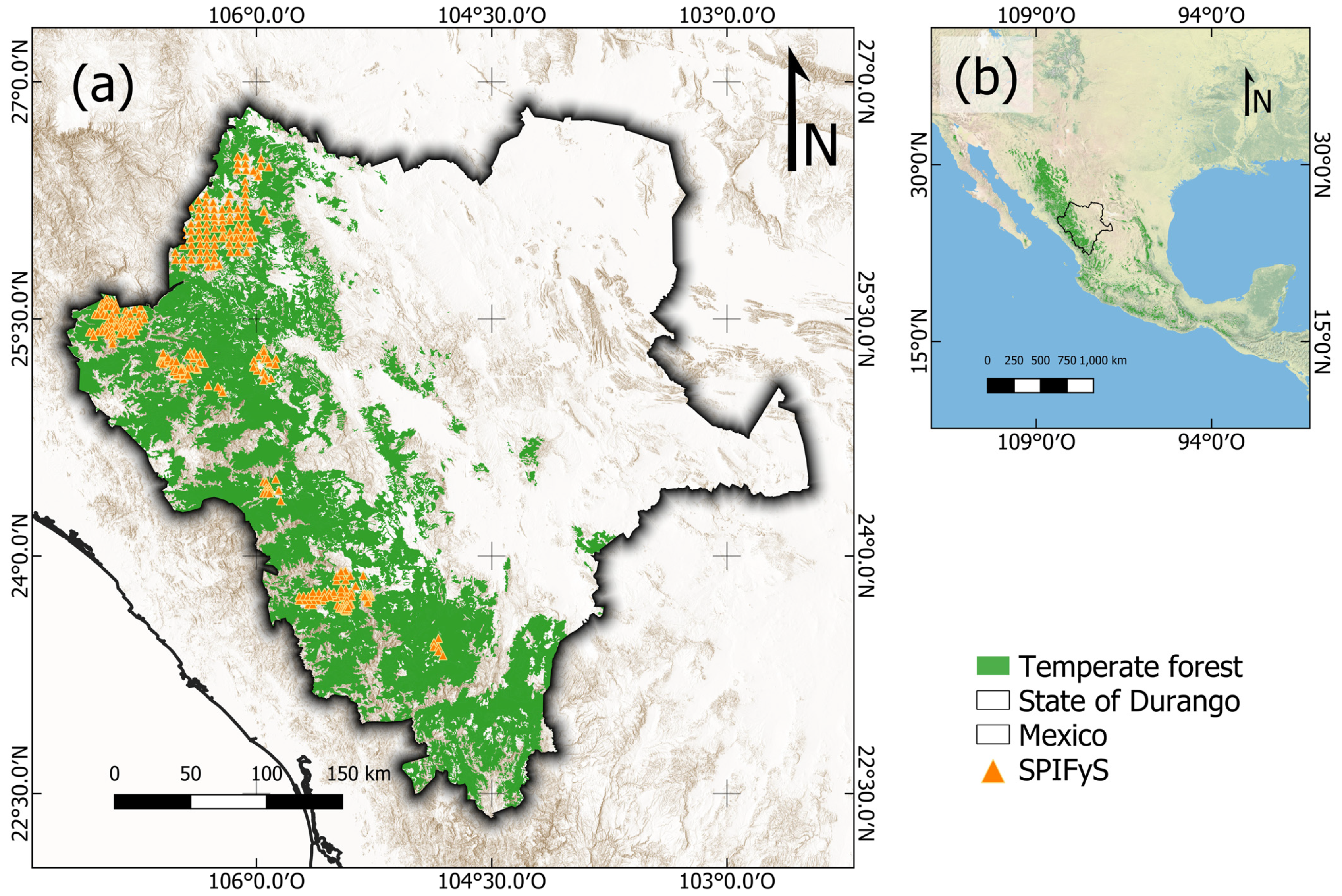
2.1. Field Data
2.2. Image Acquisition
2.3. Estimation of Land Surface Temperature (LST)
2.4. Spectral Indices
2.5. Topographic Variables
2.6. Texture Metrics
2.7. Statistical Analysis
3. Results
Model Optimization
4. Discussion
5. Conclusions
Author Contributions
Funding
Data Availability Statement
Acknowledgments
Conflicts of Interest
References
- Jiang, F.; Kutia, M.; Ma, K.; Chen, S.; Long, J.; Sun, H. Estimating the Aboveground Biomass of Coniferous Forest in Northeast China Using Spectral Variables, Land Surface Temperature and Soil Moisture. Sci. Total Environ. 2021, 785, 147335. [Google Scholar] [CrossRef] [PubMed]
- Temesgen, H.; Affleck, D.; Poudel, K.; Gray, A.; Sessions, J. A Review of the Challenges and Opportunities in Estimating above Ground Forest Biomass Using Tree-Level Models. Scand. J. For. Res. 2015, 30, 326–335. [Google Scholar] [CrossRef]
- Watson, R.T.; Noble, I.R.; Bolin, B.; Ravindranath, N.H.; Verardo, D.J.; Dokken, D.J. Land Use, Land-Use Change and Forestry; Cambridge University Press: Cambridge, UK, 2000. [Google Scholar]
- Pantaleo, Y. Tropical Reinforest above Ground Biomass and Carbon Stock Estimation for Upper and Lower Canopies Using Terrestrial Laser Scanner and Canopy Height Model from Unmanned Aerial Vehicle (UAV) Imagery in Ayer-Hitam, Malaysia. Master’s Thesis, University of Twente, Enschede, The Netherlands, 2017; 5p. [Google Scholar]
- Kumar, L.; Mutanga, O. Remote Sensing of Above-Ground Biomass. Remote Sens. 2017, 9, 935. [Google Scholar] [CrossRef]
- Holl, K.D.; Zahawi, R.A. Factors Explaining Variability in Woody Above-Ground Biomass Accumulation in Restored Tropical Forest. For. Ecol. Manag. 2014, 319, 36–43. [Google Scholar] [CrossRef]
- Ravindranath, N.H.; Ostwald, M. Carbon Pools and Measurement Frequency for Carbon Inventory. In Carbon Inventory Methods Handbook for Greenhouse Gas Inventory, Carbon Mitigation and Roundwood Production Projects; Springer: Dordrecht, The Netherlands, 2008; pp. 31–44. ISBN 978-1-4020-6547-7. [Google Scholar]
- Rodríguez-Veiga, P.; Wheeler, J.; Louis, V.; Tansey, K.; Balzter, H. Quantifying Forest Biomass Carbon Stocks From Space. Curr. For. Rep. 2017, 3, 1–18. [Google Scholar] [CrossRef]
- Zhu, X.; Liu, D. Improving Forest Aboveground Biomass Estimation Using Seasonal Landsat NDVI Time-Series. ISPRS J. Photogramm. Remote Sens. 2015, 102, 222–231. [Google Scholar] [CrossRef]
- López-Serrano, P.M.; Cárdenas Domínguez, J.L.; Corral-Rivas, J.J.; Jiménez, E.; López-Sánchez, C.A.; Vega-Nieva, D.J. Modeling of Aboveground Biomass with Landsat 8 OLI and Machine Learning in Temperate Forests. Forests 2020, 11, 11. [Google Scholar] [CrossRef]
- Zeng, Y.; Hao, D.; Huete, A.; Dechant, B.; Berry, J.; Chen, J.M.; Joiner, J.; Frankenberg, C.; Bond-Lamberty, B.; Ryu, Y.; et al. Optical Vegetation Indices for Monitoring Terrestrial Ecosystems Globally. Nat. Rev. Earth Environ. 2022, 3, 477–493. [Google Scholar] [CrossRef]
- Meneses-Tovar, C.L. NDVI as Indicator of Degradation. Unasylva 2011, 62, 39–46. [Google Scholar]
- Vaglio Laurin, G.; Pirotti, F.; Callegari, M.; Chen, Q.; Cuozzo, G.; Lingua, E.; Notarnicola, C.; Papale, D. Potential of ALOS2 and NDVI to Estimate Forest Above-Ground Biomass, and Comparison with Lidar-Derived Estimates. Remote Sens. 2016, 9, 18. [Google Scholar] [CrossRef]
- Günlü, A.; Ercanli, I.; Başkent, E.Z.; Çakı, G. Estimating Aboveground Biomass Using Landsat TM Imagery: A Case Study of Anatolian Crimean Pine Forests in Turkey. Ann. For. Res. 2014, 57, 289–298. [Google Scholar]
- Kelsey, K.; Neff, J. Estimates of Aboveground Biomass from Texture Analysis of Landsat Imagery. Remote Sens. 2014, 6, 6407–6422. [Google Scholar] [CrossRef] [Green Version]
- García-Santos, V.; Cuxart, J.; Martínez-Villagrasa, D.; Jiménez, M.A.; Simó, G. Comparison of Three Methods for Estimating Land Surface Temperature from Landsat 8-TIRS Sensor Data. Remote Sens. 2018, 10, 1450. [Google Scholar] [CrossRef]
- Van Leeuwen, T.T.; Frank, A.J.; Jin, Y.; Smyth, P.; Goulden, M.L.; van der Werf, G.R.; Randerson, J.T. Optimal Use of Land Surface Temperature Data to Detect Changes in Tropical Forest Cover. J. Geophys. Res. Biogeosci. 2011, 116, G02002. [Google Scholar] [CrossRef]
- Pongratz, J.; Bounoua, L.; DeFries, R.S.; Morton, D.C.; Anderson, L.O.; Mauser, W.; Klink, C.A. The Impact of Land Cover Change on Surface Energy and Water Balance in Mato Grosso, Brazil. Earth Interact. 2006, 10, 1–17. [Google Scholar] [CrossRef]
- Rosas-Chavoya, M.; López-Serrano, P.M.; Vega-Nieva, D.J.; Wehenkel, C.A.; Hernández-Díaz, J.C. Application of Land Surface Temperature from Landsat Series to Monitor and Analyze Forest Ecosystems: A Bibliometric Analysis. For. Syst. 2022, 31, e021. [Google Scholar] [CrossRef]
- Jaramillo, F.; Cory, N.; Arheimer, B.; Laudon, H.; van der Velde, Y.; Hasper, T.B.; Teutschbein, C.; Uddling, J. Dominant Effect of Increasing Forest Biomass on Evapotranspiration: Interpretations of Movement in Budyko Space. Hydrol. Earth Syst. Sci. 2018, 22, 567–580. [Google Scholar] [CrossRef]
- Ali, A.; Lin, S.-L.; He, J.-K.; Kong, F.-M.; Yu, J.-H.; Jiang, H.-S. Elucidating Space, Climate, Edaphic, and Biodiversity Effects on Aboveground Biomass in Tropical Forests. Land Degrad. Dev. 2019, 30, 918–927. [Google Scholar] [CrossRef]
- Mu, Q.; Heinsch, F.A.; Zhao, M.; Running, S.W. Development of a Global Evapotranspiration Algorithm Based on MODIS and Global Meteorology Data. Remote Sens. Environ. 2007, 111, 519–536. [Google Scholar] [CrossRef]
- Nguyen, H.; Wheeler, M.C.; Otkin, J.A.; Cowan, T.; Frost, A.; Stone, R. Using the Evaporative Stress Index to Monitor Flash Drought in Australia. Environ. Res. Lett. 2019, 14, 64016. [Google Scholar] [CrossRef]
- Wang, P.; Li, X.; Gong, J.; Song, C. Vegetation Temperature Condition Index and Its Application for Drought Monitoring. In Proceedings of the IGARSS 2001. Scanning the Present and Resolving the Future. Proceedings. IEEE 2001 International Geoscience and Remote Sensing Symposium (Cat. No.01CH37217), Sydney, Australia, 9–13 July 2001; Volume 1, pp. 141–143. [Google Scholar]
- Soriano-Luna, M.D.L.Á.; Ángeles-Pérez, G.; Guevara, M.; Birdsey, R.; Pan, Y.; Vaquera-Huerta, H.; Valdez-Lazalde, J.R.; Johnson, K.D.; Vargas, R. Determinants of Above-Ground Biomass and Its Spatial Variability in a Temperate Forest Managed for Timber Production. Forests 2018, 9, 490. [Google Scholar] [CrossRef]
- Mikeladze, G.; Gavashelishvili, A.; Akobia, I.; Metreveli, V. Estimation of Forest Cover Change Using Sentinel-2 Multi-Spectral Imagery in Georgia (the Caucasus). iForest 2020, 13, 329–335. [Google Scholar] [CrossRef]
- Novo-Fernández, A.; Franks, S.; Wehenkel, C.; López-Serrano, P.M.; Molinier, M.; López-Sánchez, C.A. Landsat Time Series Analysis for Temperate Forest Cover Change Detection in the Sierra Madre Occidental, Durango, Mexico. Int. J. Appl. Earth Obs. Geoinf. 2018, 73, 230–244. [Google Scholar] [CrossRef]
- Corral-Rivas, J.J.; Vargas-Larreta, B.; Wehenkel, C.; Aguirre-Calderón, O.A.; Crecente-Campo, F. Guía Para El Establecimiento, Seguimiento y Evaluación de Sitios Permanentes de Monitoreo En Paisajes Productivos Forestales; CONAFOR: Durango, Mexico, 2013; 10p. [Google Scholar]
- Vargas-Larreta, B.; López-Sánchez, C.A.; Corral-Rivas, J.J.; López-Martínez, J.O.; Aguirre-Calderón, C.G.; Álvarez-González, J.G. Allometric Equations for Estimating Biomass and Carbon Stocks in the Temperate Forests of North-Western Mexico. Forests 2017, 8, 269. [Google Scholar] [CrossRef]
- U.S. Geological Survey. Earth Resources Observation and Science (EROS) Center Science Processing Architecture (ESPA) on Demand Interface (Version 5.4). Available online: https://www.usgs.gov/media/files/eros-science-processing-architecture-demand-interface-user-guide (accessed on 16 September 2022).
- Mu, Q.; Zhao, M.; Running, S.W. Improvements to a MODIS Global Terrestrial Evapotranspiration Algorithm. Remote Sens. Environ. 2011, 115, 1781–1800. [Google Scholar] [CrossRef]
- Parastatidis, D.; Mitraka, Z.; Chrysoulakis, N.; Abrams, M. Online Global Land Surface Temperature Estimation from Landsat. Remote Sens. 2017, 9, 1208. [Google Scholar] [CrossRef]
- QGIS Development Team QGIS Geographic Information System; Open Source Geospatial. 2021. Available online: http://qgis.org (accessed on 10 February 2022).
- Rosas-Chavoya, M.; Gallardo-Salazar, J.L.; López-Serrano, P.M.; Alcántara-Concepción, P.C.; León-Miranda, A.K. QGIS a Constantly Growing Free and Open-Source Geospatial Software Contributing to Scientific Development. Cuad. De Investig. Geográfica 2022, 48, 197–213. [Google Scholar] [CrossRef]
- Sobrino, J.A.; Raissouni, N.; Li, Z.-L. A Comparative Study of Land Surface Emissivity Retrieval from NOAA Data. Remote Sens. Environ. 2001, 75, 256–266. [Google Scholar] [CrossRef]
- Rouse, J.H.; Haas, R.H.; Schell, J.A.; Deering, D.W. Monitoring Vegetation Systems in the Great Plains with ERTS. In Third Earth Resources Technology Satellite-1 Syposium; Freden, S.C., Mercanti, E.P., Becker, M., Eds.; NASA: Washington, DC, USA, 1974; Volume I. [Google Scholar]
- Oliver, M.A.; Webster, R. Kriging: A Method of Interpolation for Geographical Information Systems. Int. J. Geogr. Inf. Syst. 1990, 4, 313–332. [Google Scholar] [CrossRef]
- Horn, B.K.P. Hill Shading and the Reflectance Map. Proc. IEEE 1981, 69, 14–47. [Google Scholar] [CrossRef]
- Zevenbergen, L.W.; Thorne, C.R. Quantitative Analysis of Land Surface Topography. Earth Surf. Process. Landf. 1987, 12, 47–56. [Google Scholar] [CrossRef]
- Böhner, J.; Antonić, O. Chapter 8 Land-Surface Parameters Specific to Topo-Climatology. In Geomorphometry; Hengl, T., Reuter, H.I., Eds.; Developments in Soil Science; Elsevier: Amsterdam, The Netherlands, 2009; Volume 33, pp. 195–226. [Google Scholar]
- Rahimi, E.; Barghjelveh, S.; Dong, P. Quantifying How Urban Landscape Heterogeneity Affects Land Surface Temperature at Multiple Scales. J Ecol. Env. 2021, 45, 1–13. [Google Scholar] [CrossRef]
- Zvoleff, A. Package Glcm. R Package Version 1.6.5. 2020. Available online: https://cran.r-project.org/web/packages/glcm (accessed on 12 October 2021).
- Chen, W.; Zhang, S.; Li, R.; Shahabi, H. Performance Evaluation of the GIS-Based Data Mining Techniques of Best-First Decision Tree, Random Forest, and Naïve Bayes Tree for Landslide Susceptibility Modeling. Sci. Total Environ. 2018, 644, 1006–1018. [Google Scholar] [CrossRef] [PubMed]
- R Core Team. R: A Language and Environment for Statistical Computing; R Core Team: Vienna, Austria, 2021. [Google Scholar]
- Wood, N.S. Generalized Additive Models, 2nd ed.; Chapman and Hall/CRC: New York, NY, USA, 2017. [Google Scholar]
- Terrer, C.; Phillips, R.P.; Hungate, B.A.; Rosende, J.; Pett-Ridge, J.; Craig, M.E.; van Groenigen, K.J.; Keenan, T.F.; Sulman, B.N.; Stocker, B.D.; et al. A Trade-off between Plant and Soil Carbon Storage under Elevated CO2. Nature 2021, 591, 599–603. [Google Scholar] [CrossRef] [PubMed]
- Levine, J.; de Valpine, P.; Battles, J. Generalized Additive Models Reveal Among-Stand Variation in Live Tree Biomass Equations. Can. J. For. Res. 2021, 51, 546–564. [Google Scholar] [CrossRef]
- Frescino, T.S.; Edwards, T.C.; Moisen, G.G. Modeling Spatially Explicit Forest Structural Attributes Using Generalized Additive Models. J. Veg. Sci. 2001, 12, 15. [Google Scholar] [CrossRef]
- Latifi, H.; Fassnacht, F.; Koch, B. Forest Structure Modeling with Combined Airborne Hyperspectral and LiDAR Data. Remote Sens. Environ. 2012, 121, 10–25. [Google Scholar] [CrossRef]
- Toledo, R.M.; Santos, R.F.; Baeten, L.; Perring, M.P.; Verheyen, K. Soil Properties and Neighbouring Forest Cover Affect Above-Ground Biomass and Functional Composition during Tropical Forest Restoration. Appl. Veg. Sci. 2018, 21, 179–189. [Google Scholar] [CrossRef]
- Hasnat, G.N.T. A Time Series Analysis of Forest Cover and Land Surface Temperature Change Over Dudpukuria-Dhopachari Wildlife Sanctuary Using Landsat Imagery. Front. For. Glob. Chang. 2021, 4, 687988. [Google Scholar] [CrossRef]
- Özkan, U.; Gökbulak, F. Effect of Vegetation Change from Forest to Herbaceous Vegetation Cover on Soil Moisture and Temperature Regimes and Soil Water Chemistry. CATENA 2017, 149, 158–166. [Google Scholar] [CrossRef]
- Alrutz, M.; Gómez Díaz, J.A.; Schneidewind, U.; Krömer, T.; Kreft, H. Forest Structural Parameters and Aboveground Biomass in Old-Growth and Secondary Forests along an Elevational Gradient in Mexico. Bot. Sci. 2021, 100, 67–85. [Google Scholar] [CrossRef]
- Theofanous, N.; Chrysafis, I.; Mallinis, G.; Domakinis, C.; Verde, N.; Siahalou, S. Aboveground Biomass Estimation in Short Rotation Forest Plantations in Northern Greece Using ESA’s Sentinel Medium-High Resolution Multispectral and Radar Imaging Missions. Forests 2021, 12, 902. [Google Scholar] [CrossRef]
- Huang, S.; Tang, L.; Hupy, J.P.; Wang, Y.; Shao, G. A Commentary Review on the Use of Normalized Difference Vegetation Index (NDVI) in the Era of Popular Remote Sensing. J. For. Res. 2021, 32, 1–6. [Google Scholar] [CrossRef]
- Wang, Y.; Shen, X.; Jiang, M.; Tong, S.; Lu, X. Spatiotemporal Change of Aboveground Biomass and Its Response to Climate Change in Marshes of the Tibetan Plateau. Int. J. Appl. Earth Obs. Geoinf. 2021, 102, 102385. [Google Scholar] [CrossRef]
- Damavandi, A.A.; Rahimi, M.; Yazdani, M.R.; Noroozi, A.A. Assessment of Drought Severity Using Vegetation Temperature Condition Index (VTCI) and Terra/MODIS Satellite Data in Rangelands of Markazi Province, Iran. J. Rangel. Sci. 2016, 6, 33–41. [Google Scholar]
- Negret, B.S.; Pérez, F.; Markesteijn, L.; Castillo, M.J.; Armesto, J.J. Diverging Drought-Tolerance Strategies Explain Tree Species Distribution along a Fog-Dependent Moisture Gradient in a Temperate Rain Forest. Oecologia 2013, 173, 625–635. [Google Scholar] [CrossRef]
- Hernández-Stefanoni, J.L.; Castillo-Santiago, M.Á.; Mas, J.F.; Wheeler, C.E.; Andres-Mauricio, J.; Tun-Dzul, F.; George-Chacón, S.P.; Reyes-Palomeque, G.; Castellanos-Basto, B.; Vaca, R.; et al. Improving Aboveground Biomass Maps of Tropical Dry Forests by Integrating LiDAR, ALOS PALSAR, Climate and Field Data. Carbon Balance Manag. 2020, 15, 15. [Google Scholar] [CrossRef]
- de Meira Junior, M.S.; Pinto, J.R.R.; Ramos, N.O.; Miguel, E.P.; de Oliveira Gaspar, R.; Phillips, O.L. The Impact of Long Dry Periods on the Aboveground Biomass in a Tropical Forest: 20 Years of Monitoring. Carbon Balance Manag. 2020, 15, 12. [Google Scholar] [CrossRef]
- Blanco, A.C.; Babaan, J.B.; Escoto, J.E.; Alcantara, C.K. Modelling of Land Surface Temperature Using Gray Level Co-Occurrence Matrix and Random Forest Regression. Int. Arch. Photogramm. Remote Sens. Spat. Inf. Sci. 2020, XLIII-B3-2020, 23–28. [Google Scholar] [CrossRef]
- Iqbal, N.; Mumtaz, R.; Shafi, U.; Zaidi, S.M.H. Gray Level Co-Occurrence Matrix (GLCM) Texture Based Crop Classification Using Low Altitude Remote Sensing Platforms. PeerJ Comput. Sci. 2021, 7, e536. [Google Scholar] [CrossRef]
- Ciobotaru, A.-M.; Andronache, I.; Ahammer, H.; Radulovic, M.; Peptenatu, D.; Pintilii, R.-D.; Drăghici, C.-C.; Marin, M.; Carboni, D.; Mariotti, G.; et al. Application of Fractal and Gray-Level Co-Occurrence Matrix Indices to Assess the Forest Dynamics in the Curvature Carpathians—Romania. Sustainability 2019, 11, 6927. [Google Scholar] [CrossRef]
- Cairns, M.A.; Brown, S.; Helmer, E.H.; Baumgardner, G.A. Root Biomass Allocation in the World’s Upland Forests. Oecologia 1997, 111, 1–11. [Google Scholar] [CrossRef] [PubMed]
- Gillman, L.N.; Wright, S.D.; Cusens, J.; McBride, P.D.; Malhi, Y.; Whittaker, R.J. Latitude, Productivity and Species Richness. Glob. Ecol. Biogeogr. 2015, 24, 107–117. [Google Scholar] [CrossRef]
- Ullah, F.; Gilani, H.; Sanaei, A.; Hussain, K.; Ali, A. Stand Structure Determines Aboveground Biomass across Temperate Forest Types and Species Mixture along a Local-Scale Elevational Gradient. For. Ecol. Manag. 2021, 486, 118984. [Google Scholar] [CrossRef]
- Zhu, K.; Zhang, J.; Niu, S.; Chu, C.; Luo, Y. Limits to Growth of Forest Biomass Carbon Sink under Climate Change. Nat. Commun. 2018, 9, 2709. [Google Scholar] [CrossRef] [PubMed]
- González-Elizondo, M.S.; González-Elizondo, M.; Tena-Flores, J.A.; Ruacho-González, L.; López-Enríquez, I.L. Vegetación de La Sierra Madre Occidental, México: Una Síntesis. Acta Bot. Mex. 2012, 100, 351–403. [Google Scholar] [CrossRef]
- Ma, W.; Jia, G.; Zhang, A. Multiple Satellite-Based Analysis Reveals Complex Climate Effects of Temperate Forests and Related Energy Budget. J. Geophys. Res. Atmos. 2017, 122, 3806–3820. [Google Scholar] [CrossRef]
- Gibbard, S.; Caldeira, K.; Bala, G.; Phillips, T.J.; Wickett, M. Climate Effects of Global Land Cover Change. Geophys. Res. Lett. 2005, 32, L23705. [Google Scholar] [CrossRef]
- Strilesky, S.L.; Humphreys, E.R. A Comparison of the Net Ecosystem Exchange of Carbon Dioxide and Evapotranspiration for Treed and Open Portions of a Temperate Peatland. Agric. For. Meteorol. 2012, 153, 45–53. [Google Scholar] [CrossRef]
- Liu, L.; Wang, Z.; Wang, Y.; Zhang, Y.; Shen, J.; Qin, D.; Li, S. Trade-off Analyses of Multiple Mountain Ecosystem Services along Elevation, Vegetation Cover and Precipitation Gradients: A Case Study in the Taihang Mountains. Ecol. Indic. 2019, 103, 94–104. [Google Scholar] [CrossRef]
- Galicia, L.; López-Blanco, J.; Zarco-Arista, A.E.; Filips, V.; García-Oliva, F. The Relationship between Solar Radiation Interception and Soil Water Content in a Tropical Deciduous Forest in Mexico. CATENA 1999, 36, 153–164. [Google Scholar] [CrossRef]
- Wright, D.H. Species-Energy Theory: An Extension of Species-Area Theory. Oikos 1983, 41, 496. [Google Scholar] [CrossRef] [Green Version]


| Plot Number | Range (Mg ha−1) | Mean (Mg ha−1) | Standard Deviation (Mg ha−1) | Coefficient of Variation (%) |
|---|---|---|---|---|
| 318 | 2.05–92.34 | 31.03 | 18.14 | 0.58 |
| Row/Path | Acquisition Date | |||
|---|---|---|---|---|
| Winter | Spring | Summer | Autumn | |
| 30/43 | 4 February 2017 | 27 May 2017 | 30 July 2017 | 19 November 2017 |
| 30/44 | 4 February 2017 | 11 May 2017 | 30 July 2017 | 19 November 2017 |
| 31/42 | 11 February 2017 | 2 May 2017 | 22 August 2017 | 26 November 2017 |
| 31/43 | 11 February 2017 | 2 May 2017 | 22 August 2017 | 26 November 2017 |
| 31/44 | 11 February 2017 | 2 May 2017 | 6 August 2017 | 26 November 2017 |
| 32/42 | 2 February 2017 | 9 May 2017 | 29 August 2017 | 17 November 2017 |
| 32/43 | 2 February 2017 | 9 May 2017 | 29 August 2017 | 17 November 2017 |
| Acquisition Start and End Dates | ||||
|---|---|---|---|---|
| Row/Path | Winter | Spring | Summer | Autumn |
| MYD16A2 8/6 | 10 February 2017–17 February 2017 | 2017 May 17–2017 May 24 | 21 August 2017–28 August 2017 | 17 November 2017–24 November 2017 |
| Topographic Variable | Equation | Description |
|---|---|---|
| Elevation | Vertical distance of a point on the earth’s surface above sea level. Oliver et al. [37]. | |
| Aspect | North-facing tilt angle of the area. Horn [38]. | |
| Slope | Inclination to the horizontal. Oliver et al. [37]. | |
| Plane curvature | Direction of the slope with the highest angle. Zevenbergen and Thorne [39]. | |
| Wind Exposition Index | Calculates the wind effect in all directions. Böhner [40] |
| Texture Variables | Equation | Description |
|---|---|---|
| Mean | Mean of the probability values from GLCM. It is directly related to the spectral heterogeneity. | |
| Variance | Measure of the global variation in the image. The increase in the values, meaning higher levels of spectral heterogeneity. | |
| Homogeneity | Measure of the uniformity of grey-tones in the image. | |
| Contrast | Quadratic measure of the local variation in the images. | |
| Dissimilarity | Linear measure of the local variation in the image. | |
| Entropy | Measure of the disorder in the image. This measure is inversely related to the second moment. | |
| Second moment | Measure of the order in the image. It is related to the energy required for arranging the elements in the system. | |
| Correlation | Measure of the linear dependency between neighboring pixels. |
| Variable | Equation | Resolution (m) | Units |
|---|---|---|---|
| NDVI | (4) | 30 × 30 | −1 to 1 |
| VTCI | (5) | 30 × 30 | 0 to 1 |
| SAVI | (3) | 30 × 30 | −1 to 1 |
| LST | (1) | 30 × 30 | °C |
| Evapotranspiration | [35] | 500 × 500 | kg m−2 |
| Longitude | 30 × 30 | DD | |
| Latitude | 30 × 30 | DD | |
| Mean | Table 5 | 30 × 30 | - |
| Variance | Table 5 | 30 × 30 | - |
| Homogeneity | Table 5 | 30 × 30 | - |
| Contrast | Table 5 | 30 × 30 | - |
| Dissimilarity | Table 5 | 30 × 30 | - |
| Entropy | Table 5 | 30 × 30 | - |
| Second moment | Table 5 | 30 × 30 | - |
| Correlation | Table 5 | 30 × 30 | - |
| Elevation | 30 × 30 | meters | |
| Aspect | Table 4 | 30 × 30 | grades |
| Slope | Table 4 | 30 × 30 | grades |
| Plane curvature | Table 4 | 30 × 30 | 1/100 of z |
| WEI | Table 4 | 30 × 30 | 5 to −5 |
| Variable | edf | Residual_df | Deviance Explained | Adjusted R2 | p-Value |
|---|---|---|---|---|---|
| NDVI | 3.08 | 3.99 | 48.1% | 0.469 | <0.001 |
| LST | 6.32 | 8.04 | 38.9% | 0.384 | <0.001 |
| GLCM_mean | 2.73 | 3.46 | 34.9% | 0.342 | <0.001 |
| SAVI | 1.38 | 1.67 | 34.0% | 0.336 | <0.001 |
| GLCM_variance | 1.86 | 2.36 | 34.0% | 0.335 | <0.001 |
| Lon | 6.50 | 7.62 | 24.3% | 0.223 | <0.001 |
| Lat | 8.13 | 8.77 | 21.8% | 0.192 | <0.001 |
| ET | 1.00 | 1.00 | 12.5% | 0.113 | <0.001 |
| VTCI | 9.29 | 11.05 | 10.6% | 0.101 | <0.001 |
| Curvature | 1.95 | 2.52 | 3.30% | 0.021 | 0.125 |
| Elevation | 1.93 | 2.45 | 2.78% | 0.020 | 0.057 |
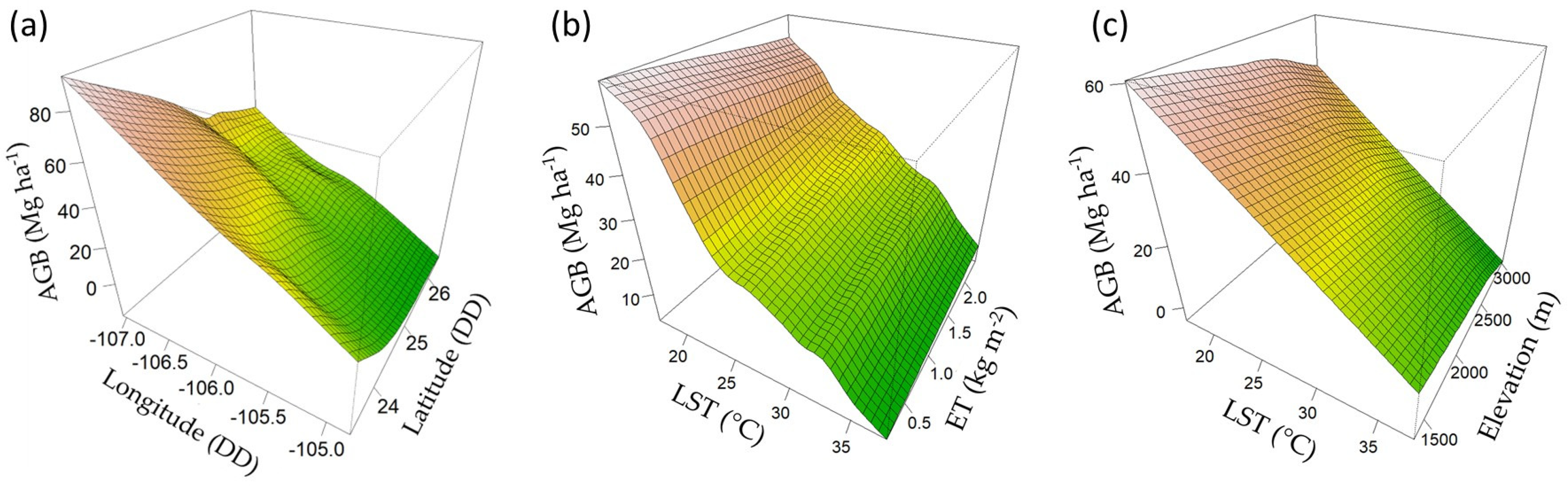
| Interaction Terms | edf | Residual_df | Deviance Explained | R2 | p-Value |
|---|---|---|---|---|---|
| LST-Elevation | 2.87 | 3.52 | 36.6% | 0.39 | <0.001 |
| LST-ET | 9.85 | 13.21 | 36% | 0.35 | <0.001 |
| Lon-Lat | 11.94 | 15.58 | 33% | 0.30 | <0.001 |
| LST-Slope | 4.27 | 5.83 | 30.5% | 0.27 | <0.001 |
| No | Model Structure | Deviance Explained | AIC | RMSE |
|---|---|---|---|---|
| 1 | AGB = s(lon,lat) + s(LST) + s(VTCI) + s(ET) + s(Elevation) + s(slope) + s(GLCM_mean) | 53.7% | 2005.72 | 30.88 |
| 2 | AGB = s(lon,lat) + s(NDVI) + s(Elevation) + s(slope) + s(GLCM_mean) | 56.8% | 2005.72 | 30.01 |
| 3 | AGB = s(lon,lat) + s(VTCI) + s(NDVI) + s(ET) + s(Elevation) + s(slope) + s(GLCM_mean) | 56.8% | 1998.27 | 29.81 |
| 4 | AGB = s(lon,lat) + s(NDVI)) + s(ET) + s(Elevation) + s(slope) + s(GLCM_mean) | 56.3% | 1995.56 | 29.80 |
| 5 | AGB = s(lon,lat) + s(LST) + s(VTCI) + s(NDVI) + s(ET+ s(Elevation) + s(slope) + s(GLCM_mean) | 60.2% | 1996.01 | 29.41 |
| 6 | AGB = s(lon,lat) + s(LST,ET) + s(LST, Elevation) + s(VTCI) + s(NDVI) + s(slope) + s(GLCM_mean) | 61.0% | 1994.34 | 28.33 |
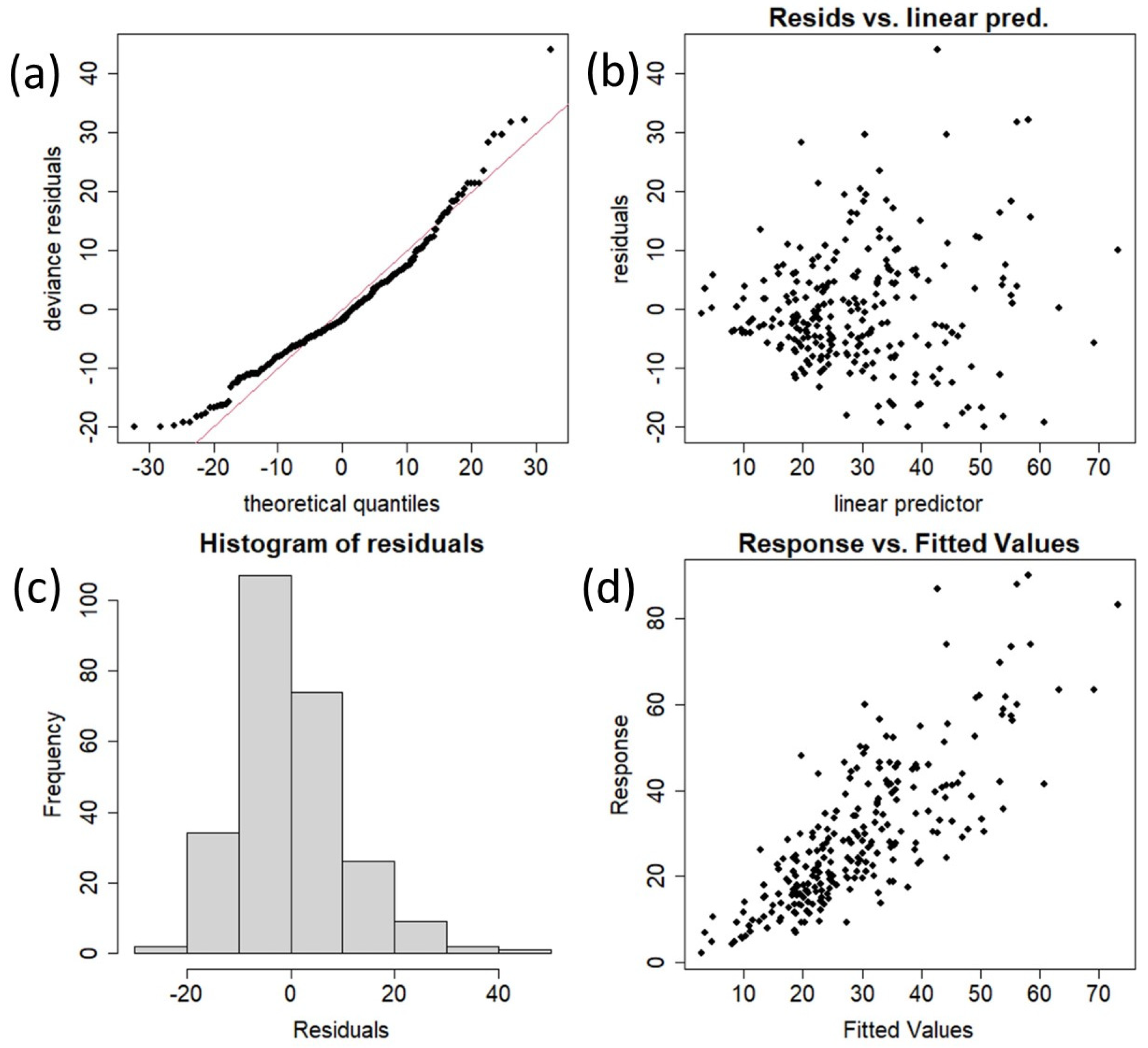
| Estimated AGB | Num. of Observations | Min | Max | Mean | SD | R2 | RMSE |
|---|---|---|---|---|---|---|---|
| GAM calibration | 318 | 2.05 | 92.33 | 30.82 | 18.00 | 0.61 | 28.33 |
| Independent verification | 50 | 4.79 | 83.25 | 27.23 | 18.15 | 0.58 | 31.21 |
Disclaimer/Publisher’s Note: The statements, opinions and data contained in all publications are solely those of the individual author(s) and contributor(s) and not of MDPI and/or the editor(s). MDPI and/or the editor(s) disclaim responsibility for any injury to people or property resulting from any ideas, methods, instructions or products referred to in the content. |
© 2023 by the authors. Licensee MDPI, Basel, Switzerland. This article is an open access article distributed under the terms and conditions of the Creative Commons Attribution (CC BY) license (https://creativecommons.org/licenses/by/4.0/).
Share and Cite
Rosas-Chavoya, M.; López-Serrano, P.M.; Vega-Nieva, D.J.; Hernández-Díaz, J.C.; Wehenkel, C.; Corral-Rivas, J.J. Estimating Above-Ground Biomass from Land Surface Temperature and Evapotranspiration Data at the Temperate Forests of Durango, Mexico. Forests 2023, 14, 299. https://doi.org/10.3390/f14020299
Rosas-Chavoya M, López-Serrano PM, Vega-Nieva DJ, Hernández-Díaz JC, Wehenkel C, Corral-Rivas JJ. Estimating Above-Ground Biomass from Land Surface Temperature and Evapotranspiration Data at the Temperate Forests of Durango, Mexico. Forests. 2023; 14(2):299. https://doi.org/10.3390/f14020299
Chicago/Turabian StyleRosas-Chavoya, Marcela, Pablito Marcelo López-Serrano, Daniel José Vega-Nieva, José Ciro Hernández-Díaz, Christian Wehenkel, and José Javier Corral-Rivas. 2023. "Estimating Above-Ground Biomass from Land Surface Temperature and Evapotranspiration Data at the Temperate Forests of Durango, Mexico" Forests 14, no. 2: 299. https://doi.org/10.3390/f14020299