Article

Forest Insect Outbreak Dynamics: Fractal Properties, Viscous Fingers, and Holographic Principle

1
V.N. Sukachev Institute of Forest SB RAS, 660036 Krasnoyarsk, Russia
2
Krasnoyarsk Scientific Center SB RAS, 660036 Krasnoyarsk, Russia
3
Department of Ecology and Nature Management, Siberian Federal University, 660041 Krasnoyarsk, Russia
4
Institute of Systematics and Ecology of Animals, Siberian Branch of Russian Academy of Sciences SB RAS, 630091 Novosibirsk, Russia
5
Institute of Biophysics SB RAS, 660036 Krasnoyarsk, Russia
*
Author to whom correspondence should be addressed.
Forests 2023, 14(12), 2459; https://doi.org/10.3390/f14122459
Submission received: 22 October 2023 / Revised: 13 December 2023 / Accepted: 15 December 2023 / Published: 18 December 2023
(This article belongs to the Special Issue Ecology and Management of Forest Pests—Series II)

Abstract

:
During the growth of a forest insect outbreak epicenter, there are processes that involve the formation and expansion of the primary epicenter of forest damage, as well as secondary epicenters—both connected and unconnected to the primary one. This study characterizes outbreak epicenters in terms of their fractal dimensions and “viscous finger” parameters at the epicenter boundary, highlighting their significance in the context of forest insect management. Local outbreak epicenters were found to be characterized by fractal dimension D = 1.4–1.5, and the boundaries of the epicenters were described using the “viscous finger” model. Proposed models were constructed and validated using remote sensing data obtained from MODIS and Sentinel-2 satellites at epicenter sites and boundaries during the outbreak of the Siberian silk moth Dendrolimus sibiricus Tschetverikov from 2014 to 2020 in the Krasnoyarsk region of Russia. The study revealed that the frequency of the mode spectrum of one-stage spatial series of “viscous fingers” corresponds with the data on the development of the outbreak foci area.

1. Introduction

Outbreaks of forest insects develop in various types of epicenters: primary epicenters, within which population densities of the pests increase, and secondary epicenters, which emerge because of the local migrations of the insects in the forest. In addition, there are migratory epicenters, which are located rather far away from the primary epicenter, resulting from the mass migrations of adult insects. It is assumed that the pre-imago stages of the pests are relatively sedentary and that only adult insects are able to migrate over considerable distances. The primary, secondary, and migratory epicenters taken together represent the insect outbreak epicenter, which is characterized by a certain total area. The damage done to forest stands and their death are determined by the dynamics of outbreak epicenter development [1].
However, it is often difficult to analyze directly the state of the insect populations during an outbreak. For example, in boreal forests of Siberia, which cover an area of about 2.7 million km2, the average density of the stable, sparse population of the major forest pest—the Siberian silk moth—may be less than 0.001 larvae per tree. Therefore, it is virtually impossible to find the larvae of this pest in a local forest [2]. Although at the outbreak peak, the population density may reach about 10,000 larvae per tree, i.e., the pest density may increase by seven orders of magnitude, forecasts of future outbreaks cannot be based on insect counts. In hard-to-reach taiga forests with a very low human population, entomological studies are usually started only when insect damage to the tree stands is serious enough to be visible from space. The effects of parasites on insect population dynamics can be estimated only in high-density populations. Moreover, even if the primary epicenter of the outbreak is detected in the Taiga region, it can only be reached by helicopter. Hence, remote sensing is the only tool for monitoring and forecasting insect outbreaks.
Point modeling, which considers the population as an aggregate, only takes into account the total population size, and ignores the distribution of the insects over the outbreak area, is usually limited to analyzing the type of spatial distribution of insects on study plots. The random, uniform, and aggregative types of distribution of insects in the forest stand are identified. Numerous aggregation indices are used to quantify the spatial distribution of insects [3].
A more detailed analysis of the spatial structure of forest insect populations is based on investigating spatial coherence between outbreaks of forest insects and the landscape features of the area and forest stand composition. The studies based on the data on outbreaks of Malacosoma disstria Hübner (Lepidoptera: Lasiocampidae) reconstructed for nearly 100 years (1928 to 2006) demonstrated more synchrony and higher intensity of outbreaks in the regions with the greater abundance of host trees [4,5,6,7,8]. Outbreaks were more synchronous and cyclic in the controlled zones, with greater proportions of aspen and other deciduous host trees, compared to wild nature where coniferous species prevailed. Yet, asynchronous outbreak dynamics were observed in the study area as well. Studies on this subject, e.g., a case study of spruce budworm Choristoneura fumiferana Clemens, 1865 (Lepidoptera: Tortricidae) [8], were aimed at identifying the areas prone to outbreaks of different species, but they did not investigate the specific behavior and spatial dynamics of each outbreak. Mathematical tools for such analyses—multivariate regression analysis and autocorrelation analysis—have been adequately developed.
The spatial distribution of insect species has been recently analyzed using an approach that combines network theory and complexity theory. This approach was implemented in the case study of the emerald ash borer bark beetle in Ontario, Canada, using geospatial datasets [9]. Another approach employed in research on spatial dynamics of forest insect outbreaks is an analysis of spatial cross-correlations among temporal changes of the outbreak areas on a vast territory [10]. This approach is used to reveal synchrony and time shifts among outbreaks of the same species in the area.
The most complex approach, involving considerable human effort in data collection and complicated methods for data analysis, is the spatial analysis of dynamics of forest insect outbreaks that includes analysis of the shapes of outbreak boundaries, the rates of outbreak spread in woodlands, and the relationships of these parameters to landscape characteristics and the structure and species composition of forest stands. For many years, it has been technically difficult to obtain such data with accurate coordinates of dynamically changing outbreaks. At present, these parameters of outbreaks can be obtained using GPS and the data gathered by satellites and unmanned aerial vehicles [11].
To gain insight into insect migration processes, it is important to study mechanisms of outbreak epicenter formation. These mechanisms differ depending on the outbreak phase. The main characteristic of the initial outbreak phase is condensation migrations: insects move into the area where ecological conditions are the most favorable for their development and concentrate there in large numbers [1]. Thus, the primary outbreak epicenter is formed. Having damaged the trees in the primary epicenter and consumed all food resources, the insects migrate to the secondary epicenters. These epicenters can be divided into connected and unconnected migration epicenters. Connected secondary epicenters are formed at the boundaries of the outbreaks of previous years; unconnected migration epicenters are formed at certain distances from the epicenters of the previous years. The emergence of unconnected epicenters may be caused by the patchiness of the species composition of forest stands, where forest plots available for insect feeding border the plots with no host trees for the insects. The formation of such outbreak epicenters results in the patchy structure of the damaged forest stands. In terms of statistical theory, such processes can be regarded as Lévy flights [12].
As the outbreak epicenter increases, first, the existing epicenter grows and new connected damaged forest areas emerge, and, second, new unconnected secondary epicenters (islands) are formed and the outbreak epicenter of fractal dimension D appears. The formation of outbreak epicenters is associated with the migration of insects. Insects migrate and continuously change their habitats because they search for food: food resources in local epicenters are often consumed completely, and insects need to find new forest stands with available food [1].
The existing remote sensing data can serve as the basis for developing models that would be used to analyze the dynamics of outbreak epicenters and changes in their shapes over time. The present study discusses approaches to describing the development of epicenters of forest insect outbreaks.

2. Materials and Methods

2.1. Study Site

The study considered the spatial structure of outbreaks of the Siberian silk moth Dendrolimus sibiricus Tschetverikov, 1908 (Lepidoptera: Lasiocampidae). The Siberian silk moth is an endemic species in the forests of Siberia, the Russian Far East, and North China. The adults of this species are good flyers, which have regular outbreaks in vast areas, during which they may damage and kill tree stands [13,14,15,16,17,18,19,20,21].
The construction and verification of the models were based on remote sensing data on areas and shapes of epicenters during two outbreaks of the Siberian silk moth D. sibiricus. The first outbreak was observed in mixed stands of the Siberian fir Abies sibirica Ledeb. and the Siberian pine Pinus sibirica Du Tour, 1803 in the Yeniseisk District of Krasnoyarsk region (58°52′–59°15′ N, 90°38′–91°10′ E) [22]. Visible defoliation was observed in 2014; by 2020, the damage had stopped increasing, and the outbreak had subsided. The total area of the completely and partly defoliated tree stands was about 800,000 ha.
The second outbreak was observed in the mixed fir–pine stands of the Sayan Mountains in the Irbey District of Krasnoyarsk Region (south of Middle Siberia, 54°45′–55°05′ N, 95°20′–99°10′ E). Dark coniferous stands dominate in this area: Siberian pine (P. sibirica), fir (A. sibirica), and spruce (Picea obovata Ledeb.). Deciduous species (Populus tremula L. and Betula spp.) occupy about 15% of the area. Visible defoliation was observed in 2019; by 2021, the damage had stopped increasing, and the outbreak had subsided. The total area of the completely and partly defoliated tree stands was about 16 km2.

2.2. Data Collection

Local outbreaks were detected using remote sensing data from the MODIS and Sentinel-2 satellites. The process of measuring the area and boundaries of the insect outbreak epicenter using remote sensing data has been sufficiently well developed by now. In the present study, changes in the sizes of the outbreak epicenters in the Yeniseisk District were estimated using normalized difference vegetation index (NDVI) from MODIS satellite data. Changes in the sizes of the outbreak epicenters in the Irbey District were estimated using NDVI (Sentinel-2) data. Graphic images and the main statistical data (size, temporal dynamics, functions of distribution of vegetation indices, etc.) for the study areas were obtained using the application programming interface: apps.sentinel-hub.com/eo-browser/ (21 August 2023).

2.3. Data Analysis

Outbreaks of forest insects are associated with the formation of plots of damaged trees—outbreak epicenters. The epicenter area is determined by the pest population size, state of the trees, and landscape structure [2]. During outbreak development, the epicenters are characterized by connectivity parameters. The epicenter is connected when any two points inside the epicenter can be connected by a line within the bounds of the epicenter. However, the epicenter territory is often unconnected and includes a large number of separate damaged plots that have different damaged areas. If the outbreak dynamics is treated as the “flow” of insects across the forest territory, in the context of the percolation theory, these damaged plots can be termed “lattice animals” [23,24,25,26,27]. The study showed that during outbreaks of the Siberian silk moth, unconnected epicenters were formed. The parameters considered while analyzing these epicenters included the area distribution of the epicenters, the relationship between the epicenter area and boundary length, the shape of the epicenter boundary, and the relationship between the shape of the boundary and the growth rate of the epicenter area.
The shape of the outbreak epicenter, like the shape of any two-dimensional bounded set, is characterized by two parameters: the function of distribution of local epicenters by area and fractal dimensions of the boundaries of local epicenters [25]. To calculate the fractal dimension of the epicenter, the area of the epicenter s and the length of its boundary L (pixels) should be estimated. The area s contained with the boundary contour is fractally determined using the length of the boundary L [12,25]:
s = s 0 L α
or
ln   s = ln   s 0 + α   ln   L
Parameter D = 2 α characterizes fractal dimension of the figure [12]. The area and the length of the boundary of each lattice animal were calculated using remote sensing data and original computer programs created in the Borland Delphi environment, and on this basis, the fractal dimension D of the boundaries was estimated.
To describe epicenter boundaries, we used an ecological analog of Darcy’s model, which describes the flow of a fluid through a porous medium in a two-dimensional space [28]:
U ( x , y ) = b 2 12 η p ( x , y )
where U (x, y) is the rate of advance; η is “viscosity” of the medium; p (x, y) is the “pressure” of the population on the tree stand; and b is constant.
If the moving interface remains straight in the horizontal plane, then its position in time and space is given by the equation U = x t . In this case, the movement of the boundary is supported by the pressure gradient ∇p, which is found in Equation (4):
p j = p 0 12 η j U b 2 x U t
where p0 is constant.
In the ecological analog of Darcy’s law, the “viscosity” parameter η can characterize a value proportional to the time required for the defoliation of the host plant in the epicenter and outside it (if the resistance of the host plant to insects is high, the defoliation time is long, if the resistance is low, the defoliation time is short). “Pressure” ∇p is the ratio of the insect density in the epicenter to the insect density outside it. Depending on the characteristics of Equation (4), the interface can have different shapes and be characterized by different fractal dimensions D [29,30,31]. Figure 1 shows the classification of the shapes of boundaries depending on their fractal dimension.
At high “viscosity” and low pressure (“sleeping” epicenter), the shape of the epicenter boundary will be characterized by a fractal size close to 1. When a more “viscous” medium pushes a less “viscous” one, the interface between the media is stable. If, however, a small periodic disturbance with wave number q and amplitude A(t) occurs along the y-axis:
x ( y ) = U t + A ( t ) cos ( q y )
At low viscosity and high pressure (an aggressive form of the pest with a high population density), the fractal dimension of the interface will be close to 2, and this boundary will have a large number of protrusions—“fingers”. In this case, the disturbance will be unstable, and the amplitude of the disturbance will increase with time. The largest pressure gradients will occur at the vertices of the interface, and, according to Darcy’s equation, the vertex will begin to move faster than the rest of the interface, and a small initial disturbance will develop into a rapidly growing “viscous finger.” As integral characteristics of the shape of viscous fingers, we will consider, firstly, the standard deviation σ of their heights and, secondly, the frequency of spectral density mode of the spatial series of viscous fingers.
How does one introduce an integral estimate of the boundary surface? To give an example, consider three variants of model boundaries:
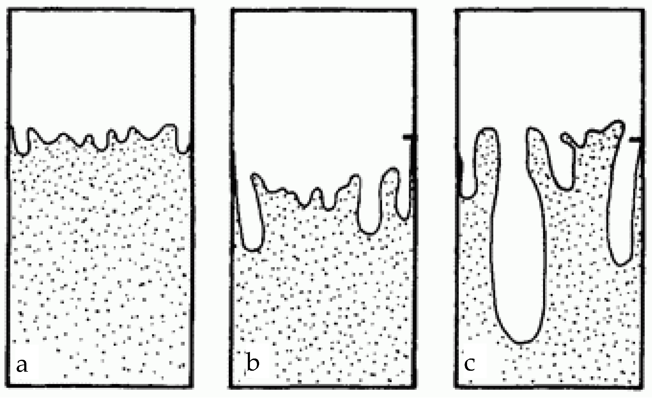
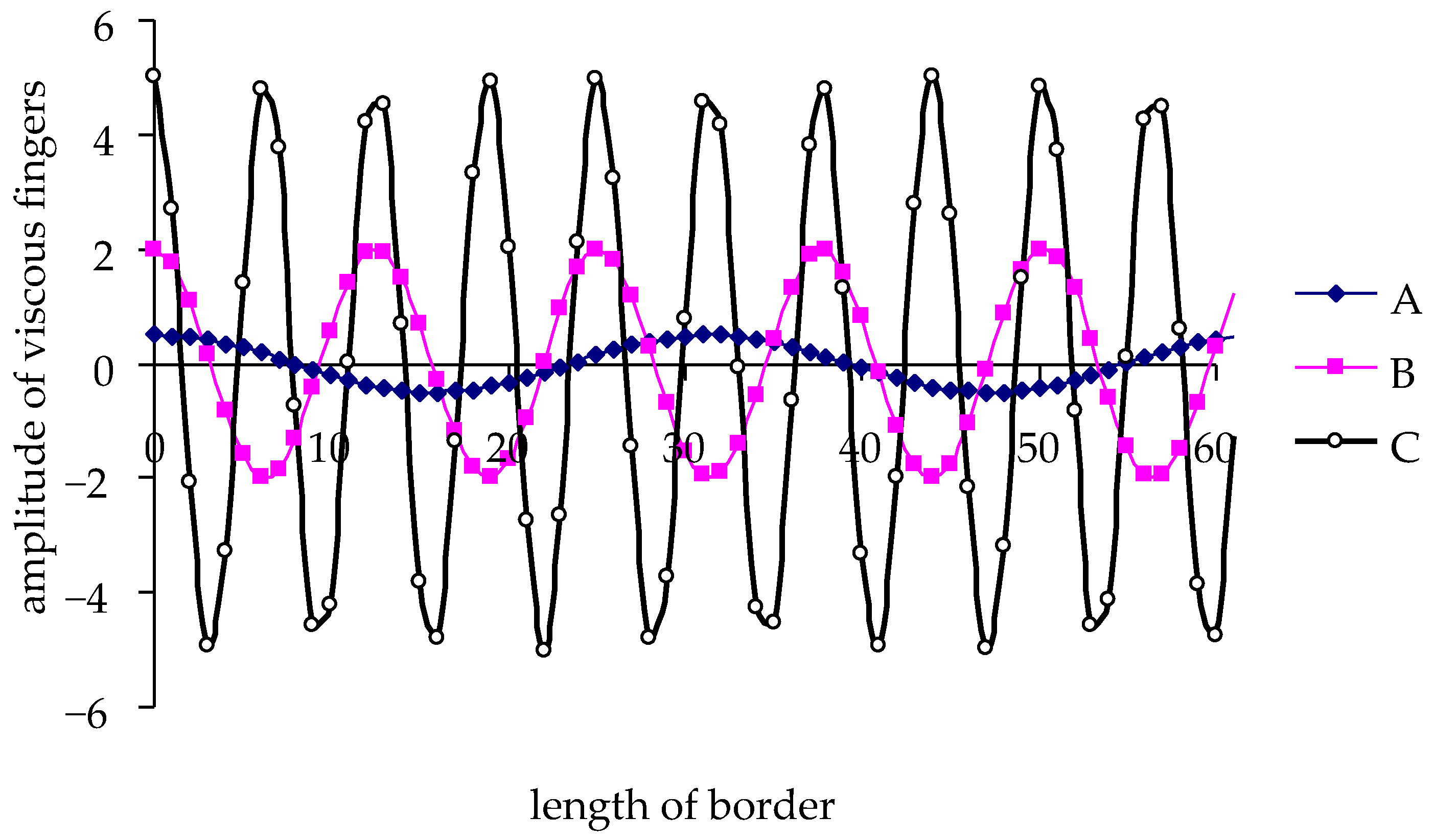
  • (A) a boundary with a small number of “viscous fingers” and small deviations from the average characteristics of the interface (type a in Figure 1);
  • (B) a boundary with an intermediate number of “viscous fingers” and moderate deviations from the average interface characteristics (type b in Figure 1);
  • (C) a boundary with a large number of “viscous fingers” and strong deviations from the average characteristics of the interface (type c in Figure 1);
  • (D) a boundary of random stationary shape.
We will use two indices as integral characteristics of the boundary: the standard deviation for a series of the boundary after removing the spatial trend and the spectrum of the series of this boundary.
Figure 2 shows a view of the boundary surface for types A, B, and C.
For each type of boundary, the spectrum of the spatial series can be estimated (Figure 3).
As can be seen from Figure 3, for the boundary with sparse viscous fingers with small amplitude (type A), the frequency of the maximum fmax of the spectral power is shifted to the region of low frequencies, and the power of the spectrum at this frequency is small. For a boundary with frequent viscous fingers with large amplitude (type C), the frequency of the maximum fmax of the spectral power is shifted to the region of higher frequencies, and the power at frequency fmax is significantly larger than that for the type A series.
Two indices can be proposed as integral characteristics of the boundary shape: the standard deviation s of the stationary spatial series and the frequency fmax (Table 1).
As follows from Table 1, type A boundaries are characterized by minimum values of shape parameters, and type C boundaries by maximum values.
If the outbreak boundary has a random D-type shape, the spectrum of this type of boundary has no pronounced maxima of spectral power at some frequency (Figure 4).
Thus, the flash boundary shape characteristics can be reasonably well estimated from the characteristics of s and fmax, as well as from the shape of the spatial series spectrum of the boundary.
To describe the dynamics and forecast the development of an outbreak of forest insects in space, let us consider the possibility of using in ecology the so-called holographic principle proposed in cosmology, which states that for a mathematical description of any world, the information contained in its outer boundary is sufficient: the idea of an object of higher dimension can be obtained from “holograms” that have a lower dimension, by analogy with a two-dimensional plate—a hologram on which a three-dimensional image of an object is recorded [32,33,34]. In the ecological case, this approach involves studying the boundaries of an epicenter with fractal characteristics D < 2 and using these characteristics to estimate the properties of a two-dimensional insect outbreak epicenter with D = 2.

3. Results

The epicenter of the Siberian silk moth outbreak in the Yeniseisk District is unconnected, consisting of a large number of micro-epicenters (lattice animals) (Figure 5). The epicenter of the Siberian silk moth outbreak in the Irbey District has a structure similar to that of local epicenters (Figure 6).
Figure 7 shows the function of density of area distribution of lattice animals (pixels).
The function f(ln s) is bimodal, and there are lattice animals with small areas (up to seven pixels), which cover about 33% of the total area of lattice animals. There are lattice animals with areas larger than seven pixels, whose area reaches approximately twenty-two thousand pixels (Figure 7). The tail of distribution with areas greater than 1000 pixels occupies about 20% of the total area of lattice animals.
Remote sensing data were used to determine areas s and perimeter lengths L of lattice animals of epicenters in the Yeniseisk District, and ln L dependences of ln s were constructed (Figure 8).
Data of calculations of Equation (2) for different outbreak epicenters in different years are presented in Table 2.
The relationship between logarithms of boundary lengths and areas of micro-epicenters in the Yeniseisk District is linear, coefficients of Equation (2) are significant according to t- and F-tests, and the equation describes this relationship very well. The coefficient of determination R2 is very close to 1, and Equation (2) takes into account over 98% of the variance of lattice animal areas. The α value characterizes the fractal dimension of lattice animals. The fact that lattice animals are described well by the general Equation (2) suggests that all lattice animals have the same fractal dimension, D = 1.33–1.36.
The relationship between the boundary lengths and areas of lattice animals was calculated, and their fractal dimensions were determined for the outbreak epicenter in the Irbey District in the same way as for the epicenter in the Yeniseisk District (Table 2). Remote sensing data were used to calculate the area and boundary length for each lattice animal. For the epicenter in the Irbey District, the fractal dimension of lattice animals is D ≈ 1.40, and the fractal dimensions of the outbreak epicenters in the Irbey and Yeniseisk Districts do not differ significantly.
The following can be said when estimating the spread rates of outbreaks of forest insects. Quantitative parameters of the boundaries should be introduced to estimate the relationships between the characteristics of epicenters and their boundaries. For this, having outlined the boundary in the image (Figure 1), we write the regression equation for coordinates X and Y of the epicenter boundary: Y = KPX (Figure 9).
After that calculation, the coordinates of the epicenter boundaries were altered using the transformation Z = Y ( X ) ( K P X ) . The results of that transformation are presented in Figure 10.
The boundary of the outbreak is shaped as protrusions and depressions—“viscous fingers”. As integrated parameters of the boundary, we will use power W of the spectrum of boundary length, regarded as an analog of the time series, frequency fmax of the spectrum (at the maximum frequency equal to the Nyquist frequency fN = 1/2 of the folded spectrum), which characterizes the maximum spectral power [35], and period λ of “viscous fingers”—the value inverse to the fmax value. These values for the boundaries in the Irbey Districts are given in Table 3.
From Table 3, it follows that before the outbreak began in 2018, when there was no damage, no viscous fingers were observed. In 2019, at the beginning of the outbreak, when about 20% of the considered territory was damaged, viscous fingers were characterized as frequent (fmax = 0.0077) and with a high height (σ = 57.2). By the end of 2020, the characteristics of viscous fingers decreased to fmax = 0.0031 and σ = 37.5. The following can be said regarding the shape of the foci in 2021 when the outbreak stopped. The parameters of the viscous fingers observed in 2021 decreased to the values fmax = 0.0002 and σ = 20.2. Comparing the dynamics of the shapes of viscous fingers, we can say that, in 2019, the shape of viscous fingers was characterized in Figure 1c; in 2020, the shape of viscous fingers was characterized in Figure 1b; and in 2021—Figure 1a.

4. Discussion

Most previous studies of tree-insect interactions using satellite-based methods [36,37,38,39,40,41,42] and unmanned aerial vehicles [43,44,45] have focused on analyzing changes in spectral characteristics of stands in the early stages of insect damage to trees. Using data from seasonal dynamics of vegetation indices is preferable to individual observations for early detection of damage with a probability of p = 0.75 of separating healthy and damaged stands [42]. However, these methods cannot identify areas that will be attacked by insects in the near future as they are time-lagged. Assessments of forest health using such methods cannot be used to identify areas that will be attacked by insects in the near future as they cannot be used to identify areas that will be attacked by insects in the near future. The use of remote sensing methods in this context solely measures damage extent, which is significant for forest economics and inventory purposes but not for forest protection. The development of remote observation methods has made it possible to analyze the spatial dynamics of outbreaks. However, works analyzing the spatial dynamics of outbreaks often use point models that only consider the total area of outbreaks and do not assess the shape of foci and their boundaries [46,47,48,49]. Unlike the mentioned approaches, the suggested method enables the identification of the potential damage zone even before the insects start to affect the forest.
To effectively counteract the negative effects of outbreaks, it is important to have reliable models to identify areas at high risk of tree mortality. For such models to accurately estimate insect-induced damage and mortality in stands, information on stand structure, environmental factors, and differences in topography must be taken into account [50]. Pest population growth is usually modeled using population or system dynamics at the stand level [51,52,53]. Nevertheless, it is difficult to estimate population growth characteristics in large forest stands. Therefore, most models for predicting the risk of insect infestation are built based on a combination of variables related to forest stand characteristics and variables determined by insect impacts. This approach has been described in [50,54,55,56]. Outbreaks have been shown to be caused by factors at several levels, in particular, the abundance of insect pests in stands, landscapes, and climatic influences at the regional level [57,58,59].
Successful pest management requires a comprehensive, quantitative approach to pest outbreaks. This approach describes pest distribution as a function of landscape topology and host-pest interactions. This perspective can be formalized via a mathematical model for multiscale outbreak dynamics, resulting in enhanced prediction and effective preventive actions to mitigate losses due to outbreaks. The achievement of this aim employs the increased availability of high-resolution spatial data on pest outbreaks by linking observed data to multiscale network theory [60]. The study of insect outbreaks through remote sensing techniques has a well-established research history [61,62]. Considerable effort has been directed toward the identification and monitoring of insect pests in agriculture and forestry [39,63,64,65]. Plant stress symptoms caused by insects, such as defoliation, can be readily detected through remote sensing techniques. These techniques have long been applied for indirect insect detection [39,61,64]. For instance, researchers have utilized satellite-obtained NDVI data to chart the spatial and temporal patterns of forest defoliation caused by the caterpillars of various phyllophagous species [66,67,68] and bark beetles [69,70]. Prompt identification of defoliation pests is facilitated using high temporal resolution data [71]. It is important to note that in these studies, damage detection is delayed relative to the time of outbreak onset and does not predict outbreak spread, although some models of outbreak dynamics are considered [47,72,73].
The authors in [73] present a spatially dynamic model of the interaction between mountain pine beetles and forests that takes into account chemical ecology, beetle redistribution, attack, and resulting host mortality. The model comprises six coupled partial differential equations with seven state variables and 20 parameters. This set of equations outlines the temporal dynamics of the following: the attraction of beetles based on pheromone concentration, fluctuations in the populations of flying and nesting beetles, the susceptibility or resistance of trees to attack, and the recovery of trees after attack. Additionally, spatial dynamics are simulated through the movement of beetles in response to gradients of pheromones and kairomones, as well as random redistribution in the absence of semiochemicals. It is challenging to evaluate the accuracy of a model that necessitates determining 20 free parameters beforehand. However, the absence of additional research on this model does not favor its validity.
A set of probabilistic models for cellular transitions was created by Zhou and Liebhold [72] to examine the spatial dynamics of gypsy moth (Lymantria dispar (Linnaeus)) defoliation. Technical terms were explained upon first use. The models consisted of four classes: simple Markov chains, rook and queen movement neighborhood models (which obviously characterize the type of spatial dynamics used in the models), and distance-weighted neighborhood models. Historical maps of gypsy moth defoliation in Massachusetts from 1961 to 1991 were digitized into a binary raster matrix and used to estimate transition probabilities. The analysis revealed that the distance-weighted neighborhood model performed better than other neighborhood models and a simple Markov chain.
The most significant difference between the present approach and the works cited above is the novel approach to analyzing the dynamics of outbreak development. The estimation of the fractal structure of the outbreak, “viscous finger” analysis, and the holographic principle of the relationship between the characteristics of foci and their boundaries have not previously received attention in the field of forest entomology. These methods have only been explored in hydrodynamics and cosmology, as is evident from our citation list. Thus, comparing our data to earlier studies proves challenging.
The present study can be considered one of the possible approaches to modeling the dynamics of outbreaks of forest insects. In contrast to fairly well-studied point models of the population dynamics of forest insects, there are no generally accepted models yet for assessing and predicting the growth processes of outbreak epicenters.
This is largely due to the uncertainty in describing the mechanisms of epicenter formation. In classical models describing the seizure of territory by a certain gene [74,75], the colonized area is, by definition, assumed to be connected. In the diffusion model, the colonized territory is also connected. However, observations show that real epicenters are unconnected, and models that take into account these aspects of the process of pest invasion are needed.
Perhaps the preference for point models over distributed models in analyzing the spatial dynamics of outbreaks is due to the difficulty of using partial differential equation models, as discussed in [74,75]. However, it should be noted that real local outbreak zones are often not connected with each other, making the use of partial differential equation techniques challenging. The proposed approach for describing the spatial dynamics of outbreaks utilizes the fractal, viscous finger, and holographic models. These models describe spatial dynamics using algebraic equations, simplifying the representation and use of field data.
However, some aspects remain unclear even with this approach. In the theory of the growth of insect outbreak epicenters is the relationship between the growth rate and shape of the epicenter boundaries and the appearance of “viscous fingers” at the boundary. The initial analysis conducted in this study suggests that such a relationship may exist, but further research is needed to assess this relationship accurately. The results of this work indicate that remote sensing data can be successfully used to describe and model the dynamics of an outbreak epicenter. An important question is whether there is a critical value of the epicenter area and its critical fractal dimension. If such characteristics exist, then at values below critical values, no outbreak development will occur.
The current study demonstrated that the outbreak epicenters of the same species, the Siberian silk moth, were characterized by the fractal dimension D = 1.3–1.4. However, it is unclear whether there really is a species-specific fractal dimension of the outbreak epicenters of individual insect species or whether this fractal dimension is determined by the landscape features and the spatial distribution of tree species in the stands.
From the analysis of the relationships between the area and the length of the boundaries of local outbreaks, we can conclude that disconnected outbreak zones can be called self-similar, and when the area of the outbreaks increases, it looks exactly the same as before the increase. Indeed, the relationship between the area and the length of the boundaries of local outbreaks does not change when the areas of these outbreaks change. How can one explain the self-similarity of local outbreaks? The first possible assumption may be that we are dealing with a mixed forest, and the shape of the boundaries depends on the heterogeneity of the forest species composition in space. However, the proportion of deciduous trees in the studied territories is quite small, and, for example, for the Irbeysky district, birches and aspens are concentrated in the lower altitude zone of the territory, while a self-similar form of local outbreaks is observed throughout the territory at altitudes from 400 to 800 m a.s.l. The second assumption may be that the Siberian silk moth is characterized by group placement of caterpillars on trees [2], and under these conditions, with the general heterogeneity of the spatial distribution of pests, fractality and self-similarity of the outbreak’s zone will be observed for damage zone. Finally, it is possible that the self-similarity of outbreak zones is associated with the response of trees to damage to needles by insects.
Further research may define more accurately the possible mechanisms responsible for the development of epicenters of forest insect outbreaks and propose reliable models that would enable predicting the dynamics of the epicenters and possible damage to forest stands, which is very important for planning pest control measures in the forest.

5. Conclusions

The present study addressed parameters of the spatial structure of Siberian silk moth epicenters. The concept of lattice animal was introduced to describe the microstructure of damage; models of the distribution of lattice animals by area were considered, and the relationships between the length of the perimeter and the areas of lattice animals were studied. Models of “viscous fingers” describing the shape of lattice animal boundaries were examined. The outbreaks of the same species were found to have similar parameters, making it possible to estimate the growth rate of the outbreak area.

Author Contributions

Conceptualization, V.S.; Methodology, V.S. and A.K.; Software, A.K.; Validation, A.K. and Y.I.; Formal analysis, V.S., A.K., Y.I. and O.T.; Investigation, A.K. and O.T. Data curation, V.S. and A.K.; Writing—original draft, V.S.; Writing—review and editing, A.K. All authors have read and agreed to the published version of the manuscript.

Funding

This research was supported by the Russian Science Foundation (grant #23-66-10015).

Data Availability Statement

The data presented in this study are available on request from the corresponding author.

Conflicts of Interest

The authors declare no conflict of interest.

References

  1. Isaev, A.S.; Khlebopros, R.G.; Kiselev, V.V.; Kondakov, Y.P.; Nedorezov, L.V.; Soukhovolsky, V.G. Forest Insects Population Dynamics; Publishing House of the Eurasian Entomological Journal: Novosibirsk, Russia, 2009; 115p. [Google Scholar]
  2. Isaev, A.S.; Soukhovolsky, V.G.; Tarasova, O.V.; Palnikova, E.N.; Kovalev, A.V. Forest Insect Population Dynamics, Outbreaks and Global Warming Effects; Wiley and Sons: New York, NY, USA, 2017; 286p. [Google Scholar]
  3. Taylor, L.R. Assessing and interpreting the spatial distributions of insect population. Ann. Rev. Entomol. 1984, 29, 321–357. [Google Scholar] [CrossRef]
  4. Sutton, A.; Tardif, J. Dendrochronological reconstruction of forest tent caterpillar outbreaks in time and space, western Manitoba, Canada. Can. J. For. Res. 2007, 37, 1643–1657. [Google Scholar] [CrossRef]
  5. Cooke, B.J.; Roland, J. Trembling aspen responses to drought and defoliation by forest tent caterpillar and reconstruction of recent outbreaks in Ontario. Can. J. For. Res. 2007, 37, 1586–1598. [Google Scholar] [CrossRef]
  6. Cooke, B.J.; MacQuarrie, C.J.K.; Lorenzetti, F. The dynamics of forest tent caterpillar outbreaks across east-central Canada. Ecography 2012, 35, 422–435. [Google Scholar] [CrossRef]
  7. Charbonneau, D.; Lorenzetti, F.; Doyon, F.; Mauffette, Y. The influence of stand and landscape characteristics on forest tent caterpillar (Malacosoma disstria) defoliation dynamics: The case of the 1999–2002 outbreak in northwestern Quebec. Can. J. For. Res. 2012, 42, 1827–1836. [Google Scholar] [CrossRef]
  8. Robert, L.E.; Sturtevant, B.R.; Cooke, B.J.; James, P.M.; Fortin, M.J.; Townsend, P.A.; Wolter, P.T.; Kneeshaw, D. Landscape host abundance and configuration regulate periodic outbreak behavior in spruce budworm (Choristoneura fumiferana Clem.). Ecography 2018, 41, 1556–1571. [Google Scholar] [CrossRef]
  9. Anderson, T.M.; Dragicevic, S. Network-agent based model for simulating the dynamic spatial network structure of complex ecological systems. Ecol. Model. 2018, 389, 19–32. [Google Scholar] [CrossRef]
  10. Barbour, D.A. Synchronous fluctuations in spatially separated populations of cyclic forest insects. In Population Dynamics of Forest Insects; Watt, A.D., Leather, S.R., Hunter, M.D., Kidd, N.A.C., Eds.; Intercept Limited: Andover, UK, 1990; pp. 339–346. [Google Scholar]
  11. Wolter, P.T.; Townsend, P.A.; Sturtevant, B.R.; Kingdon, C.C. Remote sensing of the distribution and abundance of host species for spruce budworm in Northern Minnesota and Ontario. Remote Sens. Environ. 2008, 112, 3971–3982. [Google Scholar] [CrossRef]
  12. Schroeder, M. Fractals, Chaos, and Power Laws; W.H. Freeman and Company: New York, NY, USA, 1991; 429p. [Google Scholar]
  13. Prozorov, S.S. The silk moth in fir forests of Siberia. Proc. SibLTI. Krasn. 1952, 3, 93–132. (In Russian) [Google Scholar]
  14. Boldaruyev, V.O. Population Dynamics of the Siberian Silk Moth and Its Parasites; Buryat Publishers: Ulan-Ude, Russia, 1969; 162p. (In Russian) [Google Scholar]
  15. Epova, V.I.; Pleshanov, A.S. Zones of Severity of Phyllophagous Insects in Asian Russia; Nauka: Novosibirsk, Russia, 1995; 147p. (In Russian) [Google Scholar]
  16. Kolomiyets, N.G. Parasites and Predators of the Siberian Silk Moth; Nauka: Novosibirsk, Russia, 1962; 172p. (In Russian) [Google Scholar]
  17. Kondakov, Y.P. Siberian silk moth outbreaks. In Population Ecology of Forest Animals in Siberia; Nauka: Novosibirsk, Russia, 1974; pp. 206–265. (In Russian) [Google Scholar]
  18. Rozhkov, A.S. Outbreak of the Siberian Silk Moth and Insect Control Measures; Nauka: Moscow, Russia, 1965; 178p. (In Russian) [Google Scholar]
  19. Rozhkov, A.S. Siberian Silk Moth; Nauka: Moscow, Russia, 1963; 175p. (In Russian) [Google Scholar]
  20. Soukhovolsky, V.G.; Tarasova, O.V.; Kovalev, A.V. A modeling of critical events in forest insects populations). Rus. J. Gen. Biol. 2020, 81, 374–386. (In Russian) [Google Scholar]
  21. Yurchenko, G.I.; Turova, G.I. Siberian and White-Striped Silkworms in the Far East; DalNIILCH Puplishers: Habarovsk, Russia, 2007; 98p. (In Russian) [Google Scholar]
  22. Pavlov, I.; Litovka, Y.; Golubev, D.; Astapenko, S.; Chromogin, P. New Outbreak of Dendrolimus sibiricus Tschetv. in Siberia (2012–2017): Monitoring, Modeling and Biological Control. Contemp. Probl. Ecol. 2018, 11, 406–419. [Google Scholar] [CrossRef]
  23. Broadbent, S.R.; Hammersley, J.M. Percolation processes. I. Crystals and mazes. Proc. Camb. Philos. Soc. 1957, 53, 629–641. [Google Scholar] [CrossRef]
  24. Kesten, H. Percolation Theory for Mathematicians; Birkhauser: Boston, MA, USA, 1982; 423p. [Google Scholar]
  25. Feder, J. Fractals; Plenum Press: New York, NY, USA, 1988; 283p. [Google Scholar]
  26. Jensen, I. Enumerations of lattice animals and trees. J. Stat. Phys. 2001, 102, 865–881. [Google Scholar] [CrossRef]
  27. Hsu, H.P.; Nadler, W.; Grassberger, P. Simulations of lattice animals and trees. J. Phys. A Math. Gen. 2005, 38, 775–806. [Google Scholar] [CrossRef]
  28. Kleman, M.; Lavrentovich, O.D. Soft Matter Physics: An Introduction; Springer: New York, NY, USA, 2003; 637p. [Google Scholar]
  29. Kessler, D.A.; Levine, H. The theory of Saffman-Taylor fingers. Phys. Rev. A Gen. Phys. 1986, 33, 2621–2633. [Google Scholar] [CrossRef] [PubMed]
  30. Constantin, P.; Pugh, M. Global solutions for small data to the Hele-Shaw problem. Appear. Nonlinearity 1993, 6, 393–416. [Google Scholar] [CrossRef]
  31. Ceniceros, H.; Hou, T.Y. The singular perturbation of surface tension in Hele-Shaw flows. J. Fluid Mech. 2000, 409, 251–272. [Google Scholar] [CrossRef]
  32. Hooft, G. Canonical Quantization of Gravitating Point Particles in 2 + 1 Dimensions. Class. Quantum Gravity 1993, 10, 1653–1664. [Google Scholar] [CrossRef]
  33. Susskind, L. The world as a hologram. J. Math. Phys. 1995, 36, 6377–6396. [Google Scholar] [CrossRef]
  34. Susskind, L. The Black Hole War; Little, Brown: New York, NY, USA, 2008; 470p. [Google Scholar]
  35. Anderson, T.W. Statistical Analysis of Time Series; Wiley: New York, NY, USA, 1971; 704p. [Google Scholar]
  36. Meddens, A.J.H.; Hicke, J.A.; Vierling, L.A.; Hudak, A.T. Evaluating methods to detect bark beetle-caused tree mortality using single-date and multi-date Landsat imagery. Remote Sens. Environ. 2013, 132, 49–58. [Google Scholar] [CrossRef]
  37. Anees, A.; Aryal, J. Near-Real Time Detection of Beetle Infestation in Pine Forests Using MODIS Data. IEEE J. Sel. Top. Appl. Earth Obs. Remote Sens. 2014, 7, 3713–3723. [Google Scholar] [CrossRef]
  38. Meigs, G.W.; Kennedy, R.E.; Cohen, W.B. A Landsat time series approach to characterize bark beetle and defoliator impacts on tree mortality and surface fuels in conifer forests. Remote Sens. Environ. 2011, 115, 3707–3718. [Google Scholar] [CrossRef]
  39. Senf, C.; Seidl, R.; Hostert, P. Remote sensing of forest insect disturbances: Current state and future directions. Int. J. Appl. Earth Obs. Geoinf. 2017, 60, 49–60. [Google Scholar] [CrossRef] [PubMed]
  40. Latifi, H.; Dahms, T.; Beudert, B.; Heurich, M.; Kübert, C.; Dech, S. Synthetic RapidEye data used for the detection of area-based spruce tree mortality induced by bark beetles. GIScience Remote Sens. 2018, 55, 839–859. [Google Scholar] [CrossRef]
  41. Spruce, J.P.; Hicke, J.A.; Hargrove, W.W.; Grulke, N.E.; Meddens, A.J.H. Use of MODIS NDVI Products to Map Tree Mortality Levels in Forests Affected by Mountain Pine Beetle Outbreaks. Forests 2019, 10, 811. [Google Scholar] [CrossRef]
  42. Bárta, V.; Lukeš, P.; Homolová, L. Early detection of bark beetle infestation in Norway spruce forests of Central Europe using Sentinel-2. Int. J. Appl. Earth Obs. Geoinf. 2021, 100, 102335. [Google Scholar] [CrossRef]
  43. Dash, J.P.; Watt, M.S.; Pearse, G.D.; Heaphy, M.; Dungey, H.S. Assessing very high-resolution UAV imagery for monitoring forest health during a simulated disease outbreak. ISPRS J. Photogramm. Remote Sens. 2017, 131, 1–14. [Google Scholar] [CrossRef]
  44. Näsi, R.; Honkavaara, E.; Blomqvist, M.; Lyytikäinen-Saarenmaa, P.; Hakala, T.; Viljanen, N.; Kantola, T.; Holopainen, M. Remote sensing of bark beetle damage in urban forests at individual tree level using a novel hyperspectral camera from UAV and aircraft. Urban For. Urban Green 2018, 30, 72–83. [Google Scholar] [CrossRef]
  45. Klouček, T.; Komárek, J.; Surový, P.; Hrach, K.; Janata, P.; Vašíček, B. The Use of UAV Mounted Sensors for Precise Detection of Bark Beetle Infestation. Remote Sens. 2019, 11, 1561. [Google Scholar] [CrossRef]
  46. Gray, D.R.; MacKinnon, W.E. Outbreak patterns of the spruce budworm and their impact in Canada. For. Chronicle. 2006, 82, 550–561. [Google Scholar] [CrossRef]
  47. Foster, J.R.; Townsend, P.A.; Mladenoff, D.J. Spatial dynamics of gypsy moth defoliation outbreak and dependence of habitat characteristics. Landscape Ecol. 2013, 28, 1307–1320. [Google Scholar] [CrossRef]
  48. Meigs, G.W.; Kennedy, R.E.; Gray, A.N.; Gregory, M.J. Spatiotemporal dynamics of recent mountain pine beetle and western spruce budworm outbreaks across the Pacific Northwest Region, USA. For. Ecol. Manag. 2015, 339, 71–86. [Google Scholar] [CrossRef]
  49. Senf, C.; Campbell, E.M.; Pflugmacher, D.; Wulder, M.A.; Hostert, P. A multi-scale analysis of western spruce budworm outbreak dynamics. Landsc. Ecol. 2017, 32, 501–514. [Google Scholar] [CrossRef]
  50. Sproull, G.J.; Adamus, M.; Szewczyk, J.; Kersten, G.; Szwagrzyk, J. Fine-scale spruce mortality dynamics driven by bark beetle disturbance in Babia Góra National Park. Poland. Eur. J. For. Res. 2016, 135, 507–517. [Google Scholar] [CrossRef]
  51. Fernández, A.; Fort, H. Catastrophic phase transitions and early warnings in a spatial ecological model. J. Stat. Mech. Theor. Exp. 2009, P09014. [Google Scholar] [CrossRef]
  52. Lewis, M.A.; Nelson, W.; Xu, C. A structured threshold model for mountain pine beetle outbreak. Bull. Math. Biol. 2010, 72, 565–589. [Google Scholar] [CrossRef]
  53. Fahse, L.; Heurich, M. Simulation and analysis of outbreaks of bark beetle infestations and their management at the stand level. Ecol. Model. 2011, 222, 1833–1846. [Google Scholar] [CrossRef]
  54. Overbeck, M.; Schmidt, M. Modelling infestation risk of Norway spruce by Ips typographus (L.) in the Lower Saxon Harz Mountains (Germany). For. Ecol. Manag. 2012, 266, 115–125. [Google Scholar] [CrossRef]
  55. Kautz, M.; Dworschak, K.; Gruppe, A.; Schopf, R. Quantifying spatio-temporal dispersion of bark beetle infestations in epidemic and non-epidemic conditions. For. Ecol. Manag. 2011, 262, 598–608. [Google Scholar] [CrossRef]
  56. Stadelmann, G.; Bugmann, H.; Wermelinger, B.; Meier, F.; Bigler, C. A predictive framework to assess spatio-temporal variability of infestations by the European spruce bark beetle. Ecography 2013, 36, 1208–1217. [Google Scholar] [CrossRef]
  57. Kärvemo, S.; Van Boeckel, T.P.; Gilbert, M.; Grégoire, J.C.; Schroeder, M. Large-scale risk mapping of an eruptive bark beetle—Importance of forest susceptibility and beetle pressure. For. Ecol. Manag. 2014, 318, 158–166. [Google Scholar] [CrossRef]
  58. Seidl, R.; Müller, J.; Hothorn, T.; Bässler, C.; Heurich, M.; Kautz, M. Small beetle, large-scale drivers: How regional and landscape factors affect outbreaks of the european spruce bark beetle. J. Appl. Ecol. 2016, 53, 530–540. [Google Scholar] [CrossRef] [PubMed]
  59. Raffa, K.F.; Aukema, B.H.; Bentz, B.J.; Carroll, A.L.; Hicke, J.A.; Turner, M.G.; Romme, W.H. Cross-scale drivers of natural disturbances prone to anthropogenic amplification: The dynamics of bark beetle eruptions. Bioscience 2008, 58, 501–517. [Google Scholar] [CrossRef]
  60. Urban, D.; Keitt, T. Landscape connectivity: A graph-theoretic perspective. Ecology 2001, 82, 1205–1218. [Google Scholar] [CrossRef]
  61. Riley, J.R. Remote sensing in entomology. Annu. Rev. Entomol. 1989, 34, 247–271. [Google Scholar] [CrossRef]
  62. Nansen, C.; Elliott, N. Remote sensing and reflectance profiling in entomology. Annu. Rev. Entomol. 2016, 61, 139–158. [Google Scholar] [CrossRef]
  63. Latchininsky, A.V. Locusts and remote sensing: A review. J. Appl. Remote Sens. 2013, 7, 075099. [Google Scholar] [CrossRef]
  64. Zhang, J.; Huang, Y.; Pu, R.; Gonzalez-Moreno, P.; Yuan, L.; Wu, K.; Huang, W. Monitoring plant diseases and pests through remote sensing technology: A review. Comput. Electron. Agric. 2019, 165, 104943. [Google Scholar] [CrossRef]
  65. Filho, I.F.H.; Heldens, W.B.; Kong, Z.; de Lange, E.S. Drones: Innovative technology for use in precision pest management. J. Econ. Entomol. 2020, 113, 1–25. [Google Scholar] [CrossRef]
  66. Spruce, J.P.; Sader, S.; Ryan, R.E.; Smoot, J.; Kuper, P.; Ross, K.; Prados, D.; Russell, J.; Gasser, G.; McKellip, R.; et al. Assessment of MODIS NDVI time series data products for detecting forest defoliation by gypsy moth outbreaks. Remote Sens. Environ. 2011, 115, 427–437. [Google Scholar] [CrossRef]
  67. Olsson, P.O.; Lindström, J.; Eklundh, L. Near real-time monitoring of insect induced defoliation in subalpine birch forests with MODIS derived NDVI. Remote Sens. Environ. 2016, 181, 42–53. [Google Scholar] [CrossRef]
  68. Eklundh, L.; Johansson, T.; Solberg, S. Mapping insect defoliation in scots pine with MODIS time-series data. Remote Sens. Environ. 2009, 113, 1566–1573. [Google Scholar] [CrossRef]
  69. Hart, S.J.; Veblen, T.T. Detection of spruce beetle-induced tree mortality using high- and medium-resolution remotely sensed imagery. Remote Sens. Environ. 2015, 168, 134–145. [Google Scholar] [CrossRef]
  70. Bryk, M.; Kołodziej, B.; Pliszka, R. Changes of Norway spruce health in the Białowieża forest (CE Europe) in 2013–2019 during a bark beetle infestation, studied with Landsat imagery. Forests 2021, 12, 34. [Google Scholar] [CrossRef]
  71. de Beurs, K.M.; Townsend, P.A. Estimating the effect of gypsy moth defoliation using MODIS. Remote Sens. Environ. 2008, 112, 3983–3990. [Google Scholar] [CrossRef]
  72. Zhou, G.; Liebhold, A.M. Forecasting the spatial dynamics of gypsy moth outbreaks using cellular transition models. Landsc. Ecol. 1995, 10, 177–189. [Google Scholar] [CrossRef]
  73. Logan, J.A.; White, P.; Bentz, B.J.; Powell, J.A. Model analysis of spatial patterns in mountain pine beetle outbreaks. Theor. Popul. Biol. 1998, 53, 236–255. [Google Scholar] [CrossRef]
  74. Fisher, R.A. The Wave of Advance of Advantageous Genes. Ann. Eugen. 1937, 7, 355–369. [Google Scholar] [CrossRef]
  75. Kolmogorov, A.N.; Petrovsky, I.G.; Piskunov, N.S. A study of the equation of diffusion linked to the matter increase and its application to one biological problem. Bull. MSU Ser. A Math. Mech. 1937, 16, 1–16. (In Russian) [Google Scholar]
Figure 1. Typical boundaries of the epicenter. (a) smooth boundary of the epicenter, D = 1, (b) weakly fractal boundary of the epicenter, D > 1, (c) epicenter boundary shaped as “viscous fingers”, D → 2.
Forests 14 02459 g001
Figure 2. Shape of model spatial boundaries for type A, B and C outbreaks.
Forests 14 02459 g002
Figure 3. Spectra of model spatial series of outbreak boundary boundaries of outbreak types A, B and C.
Forests 14 02459 g003
Figure 4. Spectrum of model spatial series of D-type outbreak boundaries: 1—random series with large amplitude; 2—random series with small amplitude.
Forests 14 02459 g004
Figure 5. Epicenters of the Siberian silk moth outbreak in the Yeniseisk District (Krasnoyarsk Region) (2015), NDVI (MODIS) data.
Forests 14 02459 g005
Figure 6. Local epicenters of the Siberian silk moth outbreak (Yr. 2019) in the Irbey District NDVI (Sentinel-2) data.
Forests 14 02459 g006
Figure 7. The function of density f(ln s) of the area distribution of lattice animals in the Yeniseisk District epicenter.
Forests 14 02459 g007
Figure 8. Relationship between the logarithm of the perimeter lengths L of lattice animals and the logarithm of their area s for the outbreak epicenter in the Yeniseisk District in 2015.
Forests 14 02459 g008
Figure 9. The shape of the boundaries of the Siberian silk moth outbreak in the Irbey District.
Forests 14 02459 g009
Figure 10. Transformed representation of the boundary of the Siberian silk moth outbreak in the Irbey District as “viscous fingers”.
Forests 14 02459 g010
Table 1. Shape parameters of the model series of outbreak boundaries.
Type of Border’s FormParameters
sFmax
A0.3540.032
B1.4200.081
C3.5710.161
D10.2630.339
D20.8970.258
Table 2. Parameters of Equation (2) for Siberian silk moth outbreaks in different years.
OutbreakVariables Coeff.Std. Err.t-Testp-Value
Yeniseisk district, 2015.ln s0−0.5870.115−5.1150.000
α1.3300.02455.7050.000
adjR20.979
F3103
D1.50
Yeniseisk district, 2016.ln s0−0.7880.046−17.3110.000
α1.3620.011122.5610.000
adjR20.992
F15,021
D1.47
Irbey district, 2020.ln s0−0.8440.033−25.6530.00
α1.4280.0084169.5230.00
adjR20.99
F28,737
D1.40
Irbey district, 2020.ln s0−0.7010.026−27.4470.00
α1.3740.007194.7010.00
adjR20.986
F37,908
D1.455
Table 3. Parameters of “viscous fingers” of the boundaries of the Siberian silk moth outbreaks in the Irbey Districts.
ParameterYear
2018201920202021
Frequency of the spectrum maximum, fmax, Hz00.00770.00310.0002
Standard deviation σ of “viscous fingers” pixels057, 237.520.2
Area S of outbreaks in % relative to the total area of the territory017, 5245.5647.4
Disclaimer/Publisher’s Note: The statements, opinions and data contained in all publications are solely those of the individual author(s) and contributor(s) and not of MDPI and/or the editor(s). MDPI and/or the editor(s) disclaim responsibility for any injury to people or property resulting from any ideas, methods, instructions or products referred to in the content.

