An Advanced Software Platform and Algorithmic Framework for Mobile DBH Data Acquisition

Abstract

Rapid and precise tree Diameter at Breast Height (DBH) measurement is pivotal in forest inventories. While the recent advancements in LiDAR and Structure from Motion (SFM) technologies have paved the way for automated DBH measurements, the significant equipment costs and the complexity of operational procedures continue to constrain the ubiquitous adoption of these technologies for real-time DBH assessments. In this research, we introduce KAN-Forest, a real-time DBH measurement and key point localization algorithm utilizing RGB-D (Red, Green, Blue-Depth) imaging technology. Firstly, we improved the YOLOv5-seg segmentation module with a Channel and Spatial Attention (CBAM) module, augmenting its efficiency in extracting the tree’s edge features in intricate forest scenarios. Subsequently, we devised an image processing algorithm for real-time key point localization and DBH measurement, leveraging historical data to fine-tune current frame assessments. This system facilitates real-time image data upload via wireless LAN for immediate host computer processing. We validated our approach on seven sample plots, achieving ${}^{bb}A{P}_{50}$ and ${}^{seg}A{P}_{50}$ scores of: $90.0{\%}_{(+3.0\%)}$, $90.9{\%}_{(+0.9\%)}$, respectively with the improved YOLOv5-seg model. The method exhibited a DBH estimation RMSE of 17.61∼54.96 mm ($R^2=0.937$), and secured 78% valid DBH samples at a 59 FPS. Our system stands as a cost-effective, portable, and user-friendly alternative to conventional forest survey techniques, maintaining accuracy in real-time measurements compared to SFM- and LiDAR-based algorithms. The integration of WLAN and its inherent scalability facilitates deployment on Unmanned Ground Vehicles (UGVs) to improve the efficiency of forest inventory. We have shared the algorithms and datasets on Github for peer evaluations.

1. Introduction

Forest inventory is a systematic assessment and continuous monitoring of forest resources in a specific area, with the core objective of collecting and analyzing in-depth data on the structure, species diversity and ecological functions of forests, in order to gain a comprehensive understanding of the current state and future development potential of forests [1]. In this process, in order to obtain exhaustive information about trees, such as number, height, diameter at breast height (DBH) and species, researchers usually choose ground measurement methods to take detailed measurements on predetermined sample plots. Among them, DBH measurement occupies a crucial position in the forest survey of sample plots. By measuring the DBH, researchers can accurately assess the growth trends and structural characteristics of the forest [2]. These critical data are not only essential for the development of scientific forest management strategies, but also play an integral role in maintaining ecosystem integrity and monitoring the health of forests. Therefore, being able to accurately and efficiently measure DBH in sample plots is of far-reaching significance for improving the quality and efficiency of forest inventories [3].

In the realm of forest inventory, the measurement of DBH has long relied on traditional manual methods. For instance, foresters often use contact measuring tools such as measuring tapes or calipers to measure directly around the trunk of a tree, and then use established formulas to convert the circumference data into a DBH value. A total station is an optical measurement tool that can estimate the DBH by evaluating the angle and distance between two points. In addition, the Haglof Electronic Diameter Meter provides a simplified method. Although it is primarily used to estimate tree height, it can also be used to measure DBH under certain conditions [4,5,6]. Traditional methods of measuring DBH have proven their reliability in areas with flat terrain and a limited number of trees. However, when the demand extends to large-scale or real-time measurements, especially in complex terrain such as mountains, swamps, or dense forests, their efficiency and accuracy are seriously challenged. These challenges stem not only from the limitations of the methodology itself, but also from the complexity of operations, time constraints, and risks to personal safety in unknown environments [7,8,9]. First, traditional methods usually require complex operational procedures, which can lead to significant time and labor cost increases in large-scale measurements [10]. Second, due to time constraints, the measurement process may be compressed, which in turn affects its accuracy. Further, for trees with complex morphology or which are obscured by other vegetation and obstacles, the measurement accuracy of traditional methods may be significantly reduced [7]. In summary, although the traditional methods are still applicable under specific conditions, their limitations in a wide range and complex application scenarios cannot be ignored [10].

With the rapid development of modern technology, the emergence of advanced techniques such as LiDAR, Structure Restoration Motion (SFM) reconstruction techniques, and depth cameras have brought about unprecedented changes in the field of precision measurements. These technologies offer a rich source of information with high efficiency and accuracy of forest structure and tree parameters [11,12,13,14]. LiDAR technology, by emitting laser pulses and measuring the time of their reflection back to the ground, is capable of generating highly accurate 3D point cloud data [11]. Meanwhile, SFM technology, by analyzing 2D images from multiple viewpoints, is also able to generate corresponding 3D point cloud data [12]. Whether the point cloud data are obtained by LiDAR or SFM methods, a series of processing steps need to be followed in order to estimate the DBH of trees [15]. First, for point cloud data on irregular ground, ground filtering is required to obtain a digital elevation model (DEM) [16]. Subsequently, all point cloud data are normalized based on the DEM to obtain an approximately flat forest-like model. Next, by intercepting the point cloud at a fixed height, a subset of the point cloud with the “DBH height” of all trees in the sample plot can be obtained. Finally, the clustered subset of point clouds are fitted to circles or cylinders, respectively, and the DBH can be estimated [16,17,18,19,20,21].

Although these methods provide relatively accurate data, there are still some challenges in practical applications. For example, scanning times in some scenes via LiDAR can be as long as 40 min to 1.5 h [17], while 3D reconstruction of a sample plot of 47 to 69 trees using SFM methods can take 7 to 11 h [20]. In addition, LiDAR equipment, backpack LiDAR systems, and UAVs pose challenges for forestry surveyors to carry and maneuver in the forest due to their large size and weight (as shown in

Table 1. Key physical parameters of equipment for plot-level inventories.

Equipment Type	Equipment	Size (mm)	Weight (Kg)
Laser Scanner	Leica ScanStation2 (Leica Geosystems AG, Heerbrugg, Switzerland)	$265\times 370\times 550$	$18.5+12$ 1
LIDAR	LiteMapper 5600 2 (IGI mbH, Kreuztal, Germany)	$420\times 212\times 228$	16.0
UAV	DJI Matrice 600 Pro (DJI, Shenzhen, China)	$1668\times 1518\times 727$	9.5
RGB-D Camera	RealSense D435i (Intel, Santa Clara, CA, USA)	$90\times 25\times 25$	0.075
Laptop	Lenovo Y7000P (Lenovo, Beijing, China)	$361\times 267\times 26.9$	2.35
Router	ASUS RT-AC68U (ASUS, Taipei)	$220\times 83.3\times 160$	0.6

¹ Total weight of scanner and power supply unit.

). Offline forest inventory algorithms do not provide real-time operations, resulting in forestry surveyors not having instant access to measurement data. In addition to the limitations in operational performance, 3D unstructured point cloud data are highly variable in different scenarios. For example, in steep slope or ridge terrain point clouds, the error of ground filtering is still an unsolved problem [22]. Ground filtering algorithms are usually not able to automatically adapt to different scenes [23]. In the case of dense vegetation and complex terrain, the acquired point cloud data are not accurate, which can greatly limit the accuracy of the terrain surface, while heavily relying on empirical formulas for fitting the breast diameter for different tree species [16,20,24]. The influence of factors makes point cloud-based ground object segmentation require developers to customize the algorithms for the characteristics of different forestry plots, which is one of the most important factors limiting its versatility. Meanwhile, its popularization in large-scale applications may be limited due to the high cost of high-precision LiDAR systems and high-performance computing equipment [13].

In the current technological context, RGB-D (Red, Green, Blue-Depth) cameras represent a significant advancement over traditional imaging systems, particularly within agricultural and forestry applications [25,26]. These cameras not only capture the standard red, green, and blue (RGB) color data but also add depth information (D) by measuring the distance to objects using a sensor. This depth-sensing capability, often realized through techniques like Time-of-Flight or structured light, allows for the generation of a depth map, which, when fused with RGB data, results in a comprehensive 3D representation of the scene. The inclusion of depth data enables precise measurements of plant morphology and stand structure, offering detailed insights into canopy density and tree height. The relatively low cost and ease of operation further position RGB-D cameras as practical tools for high-resolution, large-scale data capture, providing valuable multidimensional information in real-time for various analytical and monitoring purposes [14]. Fan et al. [27] have pointed out the cost-effectiveness of RGB-D cameras compared to LiDAR systems in forest inventory and further developed an RGB-D-based SLAM system. Amelia et al. [28] calculated the dominant depth values in a given area as the “trunk depth” and then filtered the pixels whose depths were much greater than the trunk depth, thus obtaining a mask of the main trunk of the tree. Based on traditional methods, the extraction of tree trunk ROI regions is always based on a large number of rules and assumptions of target states. For example, the center axis of the tree must almost overlap with the center line of the frame, and only one tree can appear in the image. Meanwhile the rough regularity algorithm will lead to a decrease in the accuracy of segmentation, resulting in insufficient accuracy of the measured data based on the masked region. Sun et al. [29] constructed an apple tree trunk measurement system using the Azure Kinect V2 (Microsoft, Redmond, WA, USA) depth camera. They placed the depth camera on a tripod, which was connected to a computer via a data cable. Liu et al. [30] chose a computer with a Nvidia GTX-1060 (NVIDIA Corporation, Santa Clara, CA, USA) as a way to improve the real-time performance of the system for fruit detection and picking point localization. Although RGB-D camera-based vision systems for real-time computing in forestry have been widely validated in academia and have been widely used, their practical application in complex forestry environments still faces challenges. For example, the difficulty of carrying large computing platforms makes it more difficult to measure in areas that are difficult for humans to access directly. These problems are similar to those faced when using conventional measuring equipment, where the equipment is not portable.

The great success of deep learning techniques in the field of image segmentation has led to the increasing use of deep cameras in the field of agriculture and forestry. For example, Sila et al. [31] constructed an image-based tree trunk detection system for forestry mobile robots using five different neural networks. They used a detection frame to define tree trunks in the field of view, but since they did not segment the semantic information within the detection frame, the practical applications available are limited. Danilo et al. [22] imporved the U-Net by adding a deep residual module for tree segmentation in urban environments and further fitting the skeleton model of trees. In addition, Vincent [32] used Mask R-CNN and Cascade Mask R-CNN for segmenting tree images and predicting keypoint locations, in which they reported tree detection rates and segmentation accuracies of 90.4% and 87.2%, respectively. Although both studies successfully extracted the trunk masks of trees from 2D images, their algorithms still have limitations in terms of real-time performance. In order to achieve fast standing tree segmentation, Wang et al. [33] optimized the DeepLabV3+ framework to enhance the performance of edge details in tree segmentation and introduced a lightweight network, MobileNet, to reduce the computational complexity, which resulted in a significant improvement in single-frame inference speed. Instance segmentation algorithms are usually categorized into one-stage and two-stage models. Two-stage models such as Region Convolution Neural Network (R-CNN) [34], Fast-RCNN [35], and Mask R-CNN [36] show excellent performance in tasks such as forest detection, segmentation, maturity classification, and yield computation. However, networks such as Faster R-CNN suggest networks by generating regions, which improves segmentation accuracy but leads to an increase in model size and processing time, which is inconsistent with the demand for real-time and light weighting. Redmon et al. [37] proposed YOLO, a single-stage target detection model, which integrates the tasks of detection, classification and localization into a single regression problem, thus simplifying the network structure and computational cost. Based on this, the Yolact [38] model was developed, which simplifies the segmentation and localization tasks into two parallel tasks. First, it generates prototype masks that do not depend on any instances, using a similar approach to that of fully convolution networks [39]; second, it adds a target detection branch that predicts “mask coefficients” for each anchor. The final mask is generated by combining these two parts after processing through non-maximal suppression [40]. Cao et al. [41] conducted a comprehensive evaluation of the performance of multiple segmentation algorithms on the tree segmentation task, and found that the YOLO series of models performed the best in terms of comprehensive performance. All these studies verified that deep learning-based segmentation algorithms are able to quickly and accurately acquire pixel-level coordinates of tree regions in 2D images, and these algorithms show significant advantages in data acquisition and recognition accuracy compared with traditional methods.

In order to accurately measure the tree’s diameter at breast height (DBH), the acquired trunk region montages need to be further processed. The diameter-at-breast points, usually located at a height of about 1.3 m above the ground in the trunk, are two points in the tree cross-section that intersect the line connecting the center of mass [42]. The positioning accuracy of these points directly affects the accuracy of breast diameter measurements. Both traditional methods for locating breast diameter points and deep learning-based methods have their advantages and disadvantages. For example, Amelia et al. [28] used principal component analysis to determine the main axis of the trunk and traversed the binary image to determine the breast diameter points. However, this method is sensitive to noise points and may not be applicable to morphologically irregular trees. Fan et al. [27] combined the IMU sensor and SLAM method to record the spatial information of the root position of the tree so as to directly extract the cross section of the breast diameter position. However, due to the drift characteristics of the SLAM algorithm, long time measurements may lead to cumulative errors. Grondin [32] optimized Mask R-CNN by adding a key point prediction module for predicting key points on the tree trunk, but this method requires a large amount of data annotation. They have a prediction error of 5.2 pixels for the diameter points of the thorax, and this error is further amplified during the mapping of the 2D image coordinate system to the 3D world coordinate system, resulting in a large deviation in the measured thorax values.

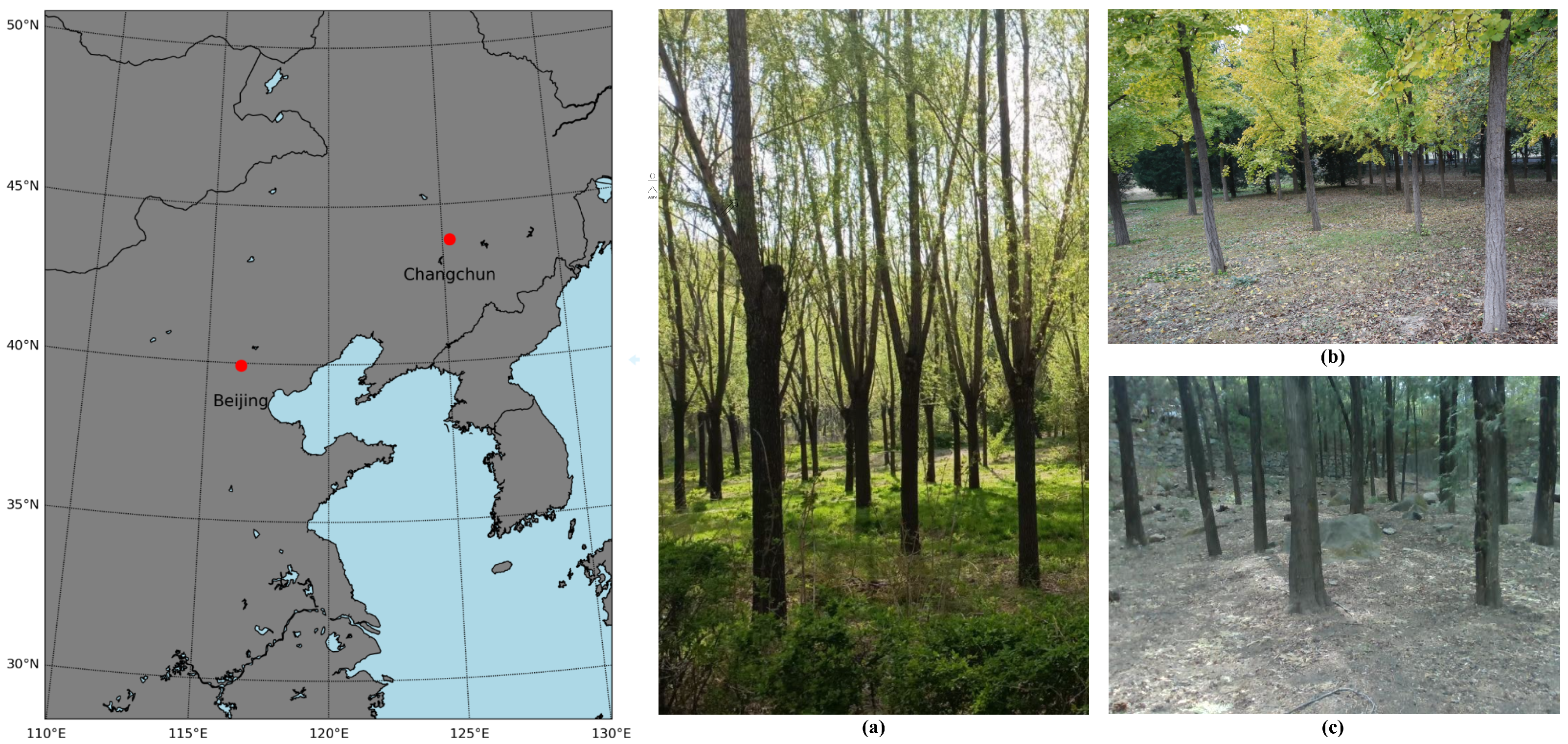
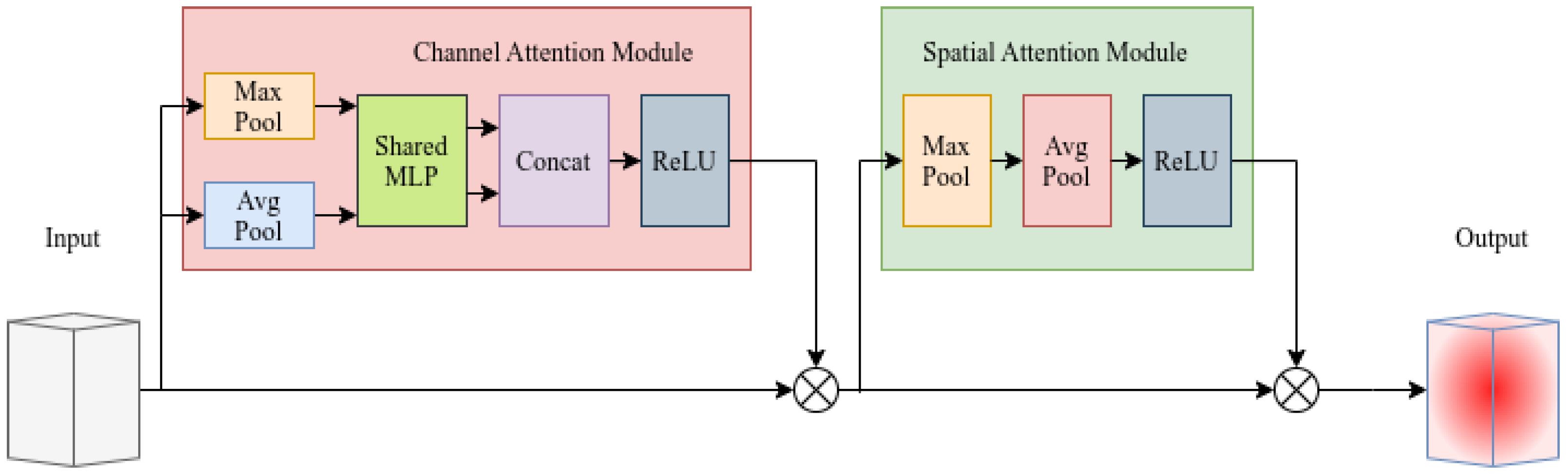
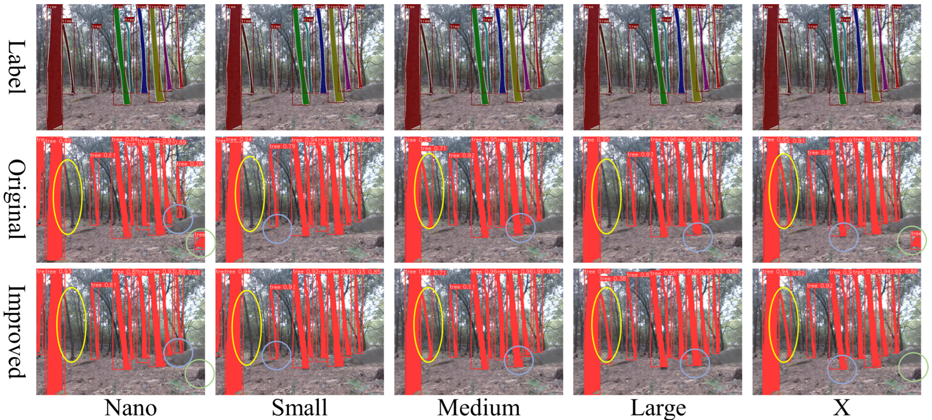
This system is not only portable, but also capable of calculating the breast diameter of trees in the field of view in real time. We have deeply optimized YOLOv5-seg, especially by introducing a Channel and Spatial Attention (CBAM)-based module, which enhances the model’s ability to identify and segment trees in complex forest environments. In addition, we propose a more robust, high real-time and multi-objective localization algorithm compared with the traditional tree breast diameter point localization method. In order to verify the effectiveness of the proposed system, we have performed the proposed system in seven different forest scenes by comparing the DBH computed by the system with the data obtained manually by the traditional method, whose average error is only 39.61 mm ($R^2=0.937$, $MAPE=6.5\%$). This result strongly suggests that the system has the potential to replace traditional chest diameter measurement tools. Considering our future research on the application of unmanned aircraft and unmanned ground vehicles to forest resource surveys and automated path planning in forests, we developed a wireless LAN-based server platform for the system, which allows users to visualize and monitor the system operation or guide the system operation remotely in real time.

2. Materials and Methods

2.1. Study Overview

In this study, we propose an advanced automated tree-breast diameter measurement system based on instance segmentation and RGB-D imaging, and its workflow is shown in Figure 1. First, a depth camera is used to capture continuous RGB frames and depth matrices of trees. This data is timestamped and verified to ensure that it was captured synchronously. They are then packaged into “Frame Pack” and transmitted to a remote platform via wireless LAN. Any received “Frame Packs” that are not in chronological order are then discarded at the remote platform. For each received “Frame Pack”, a modified YOLOv5-seg model is used to identify each tree’s pixel set in the RGB image. In the third step, data enhancement of the tree masks was performed to extract the skeleton lines of each mask. DBH key points are then localized using image processing techniques. Ultimately, the 3D coordinates of the key points are determined by mapping the image coordinates to the camera coordinate system to calculate the tree trunk diameter. The subordination of the tree in the historical data is also discriminated, and the current measurements are corrected based on the existing data of the tracked target.

2.2. Study Area and Data Acquisition

In order to validate our experiment, we selected seven forest sample plots for evaluation. Sample Plots 1 and 2 were located in Beijing Olympic Forest Park (116°23′ E, 40°2′ N). Sample Plots 3 to 5 are located in Beijing Jiufeng National Forest Park (116°5′ E, 40°3′ N). Sample Plots 6 and 7 are located in Jingyuetan National Forest Park, Changchun (125°29′ E, 46°42′ N). Both the Olympic Forest Park and the Jiufeng National Forest Park are located in Beijing and are rich in forest resources. The Olympic Forest Park is relatively flat and most of the trees are planted artificially, making it an excellent location for us to verify the effectiveness of the algorithm in our early experiments. To further validate the performance of the system in real-world environments, we chose sample plots, which are all located in naturally occurring primary forests. A sample of the experimental locations is shown in Figure 2.

Given the actual forest inventory task, different conditions of the sample sites may have different impacts on the task. In this study, representative sample plot condition types were selected, documented and categorized in detail. For detailed information on the trees to be tested and their attributes in these sample plots, please refer to

Table 2. Details of the experimental sample plots.

Site	Study Plot	Plot Type	Acqu. Dates	Dominant Species	No. Trees	Min. DBH (cm)	Max DBH (cm)	Mean DBH (cm)	Terrain Variability	Straightness	Circularity	Shading
Site A. 1	Plot 1	Plantation	18 October 2022	Ginkgo biloba	47	35.5	106	59.7	flat	Slightly Bent	Moderately Round	No
	Plot 2	Plantation	22 October 2022	Ginkgo biloba	40	31.5	90.1	59.4	flat	Slightly Bent	Moderately Round	No
Site B. 2	Plot 3	Primary Forest	25 October 2022	Pinus massoniana	30	25.2	59.9	38.2	flat	Straight	Circular	Sparse
	Plot 4	Primary Forest	25 October 2022	Pinus massoniana	30	21.3	96.4	55.6	flat	Straight	Circular	Sparse
	Plot 5	Primary Forest	25 October 2022	Pinus massoniana	30	25.9	65.7	42.0	Rolling	Straight	Circular	Sparse
Site C. 3	Plot 6	Primary Forest	11 May 2023	Salix matsudana	55	50.5	84.9	68.1	Rolling	Straight	Circular	Sparse
	Plot 7	Primary Forest	11 May 2023	Salix matsudana	47	48.0	82.0	64.8	flat	Straight	Circular	Sparse
Total	-	-	-	-	354	-	-	-	-	-	-	-

¹ Beijing: Olympic Forest Park. ² Beijing: Jiufeng National Forest Park. ³ Changchun: Jingyuetan National Forest Park.

. This study focused on the following aspects: the degree of relief of the terrain, the growth pattern of the trees, and the shading of the ground vegetation in order to evaluate the performance of our system under various sample site conditions. The degree of relief of the terrain was determined by using the level of the iPhone XS (Apple Inc., Cupertino, CA, USA) to measure and observe whether there were any obvious step-like faults in the ground. For the degree of bending of the trees, we focused on the smoothness of the skeleton, which was defined as “Highly Bent” if the skeleton line was irregularly curved at a certain point. The roundness of the tree trunks was assessed by direct observation, looking for visible depressions on the tree surface. Occlusion by vegetation on the ground surface was identified as a key factor affecting the forest survey task visually. We defined a situation where there was no vegetation cover at all as “No”, a situation where there were only small branches that did not prevent observation of the tree trunks as “Sparse”. The situation where trees are close to each other and there are dense low branches on the ground obscuring the trunks is defined as “Intense”.

In order to ensure that accurate values of DBH data were obtained for each sample plot, we manually measured the DBH of trees in each experimental plot using a tape measure. Measurement locations were selected at a horizontal cross-section of the tree trunk at 1.3 m above the ground. Each tree was measured three times independently by two researchers, and after removing obvious outliers, the average of the six measurements was taken as the final data as a way of circumventing manual measurement errors. To understand the time spent by skilled forest investigators to manually measure diameter at breast height, we timed the measurement process in the last three sample plots. Specifically, the measurements in Plot 7 took about 30 min, Plot 6 took about 77 min, and Plot 5 took about 53 min, which shows that manual measurements are time-consuming. It is worth noting that the last two plots were much more difficult to measure due to the steep terrain and dense vegetation on the surface.

The data used to train the instance segmentation model were acquired using an RGB camera (Canon EOS M50 (Canon Inc., Tokyo, Japan)) with a resolution of $6000\times 4000$ pixels, an aperture size of $f/3.5$, an exposure time of 1/80 s and the focal length of the lens was fixed to 15.0. During acquisition, we fixed the camera on a tripod with the height of the lens at about 1.3 m above the ground. When collecting woodland images, we tried to ensure that the trunks of the trees in the field of view were horizontally intact, while requiring that the roots of each tree be above the bottom of the frame. We trained on a mixture of cloudy, sunny, and hazy weather images to ensure that the model is as immune as possible to the effects of intense lighting when making inferences. We also used the Intel® RealSense™ D435i camera to capture a portion of the data, all at a resolution of $640\times 480$, to improve the model’s performance in low-resolution situations. After filtering, we obtained 387 real forest images and labeled the trees in them. We divided all the captured data into training set, validation set and test set according to the ratio of 7:2:1.

We performed data enhancement on the original dataset by expanding each training set to 51 images as shown in Figure 3. Specific information about the dataset before and after enhancement is illustrated in

Table 3. Training dataset details.

Data	Total	Train	Validation	Test
Jiufeng Forest Park	111	77	22	12
Enhanced	3961	3927	77	12
Olympic Forest Park	276	193	55	28
Enhanced	9926	9843	55	28
Total	13,887	3927	77	40

. Training was performed on Ubuntu 20.04 operating system, Python environment was built using Anaconda 3, CUDA 11.7, and YOLOv5-seg was cloned from https://github.com/ultralytics/yolov5 (accessed on 31 October 2022) During the training process of this study, we used YOLOv5-seg’s default hyper-parameter configuration file “hyp.Scratch-low.yaml”. In addition, we loaded the pre-training weights of each model provided by Ultralytics to optimize the performance of the model. The specific parameter information that was ultimately used is shown in

Table 4. Training environments.

GPU	Nividia RTX 3090 (24 GB)
CPU	Intel(R) Xeon(R) Gold 6330 CPU @ 2.00 GHz
Memory	86 GB DDR4
Optimizer	Adam
Epoch	50
Batch Size	32
Initial Learning Rate	0.001
Weight Decay	0.0005

.

2.3. Equipment and Experimental Set-Up

2.3.1. Vision-Based System

When building an efficient vision measurement system, the selection and configuration of core hardware devices is critical. These hardware usually include vision sensors (e.g., RGB cameras and depth cameras), a host computer (e.g., a computer or microcontroller) for data processing and analysis, and other necessary auxiliary devices (e.g., tripods and gimbals). In this study, our vision system consists of the following three components: first, a laptop computer equipped with an Intel i7-10750H CPU and an Nvidia GeForce RTX 2060 GPU serves as the host computer, whose powerful computational power ensures real-time data-intensive computing, and the laptop’s portability also ensures the ease of movement of the forest surveyors in the forest. Second, an Asus RT-AC68U wireless router was set up near the experimental site as a hub for data transmission. Finally, a Raspberry Pi 4 Model B running the Ubuntu operating system served as the downstream computer and was connected to an Intel® RealSense™ D435i depth camera via USB 3.0, a combination that ensured that the measurement sensors were easy to carry.

The Intel® RealSense™ D435i was chosen as the image acquisition device for the vision system based on its wide usage and excellent performance in the field of agricultural and forestry research. The camera utilizes Time-of-Flight (ToF) technology to acquire depth information, and its front end is equipped with infrared transmitter and receiver devices. By measuring the reflection time of an infrared beam, the distance of an object can be accurately calculated. At the software level, we activate the camera’s RGB and depth sensors using the C++ interface of the Intel® RealSense™ SDK 2.0 and capture $640\times 480$ color and depth frames at 30 fps. Calibration of the depth sensor to RGB was performed using the Intel® RealSense™ D400 Series Dynamic Calibration Tool.

A wireless LAN video streaming server based on TCP protocol was running in each of the two computers at the measurement end and the remote. During the run-time of the vision measurement system, the two computers are in constant communication, which is described in detail in the Section 2.5 (The implementation of our system is illustrated in Figure 4).

2.3.2. Experimental Procedure

During the experiment, a wireless router first needs to be deployed near the plot so that the wireless communication module built into the Raspberry Pi can upload the captured images to a remote computer. Subsequently, the Raspberry Pi equipped with a depth camera was activated. Once it is successfully connected to the wireless LAN, the listening module starts responding and waiting for a connection request from the remote end. Upon receiving the request from the remote server, the server activates the camera module and starts the network upload. Successful reception and real-time display of images by the server side marks the successful startup of the system. The server will automatically process each received frame, and after successfully measuring the DBH value of the tree in the frame, it will directly mark the DBH key points, the line at breast height, and the number of the tree in the current frame on the corresponding position of the trees. In the upper-left corner of the screen, the number of visible trees in the current frame, the number of trees that can be measured, and the DBH values and distance information of the corresponding trees are displayed according to their ID.

In the actual data collection phase, the step path of the collector not only affects the time efficiency of data collection, but also has an indirect impact on the accuracy of data. In order to ensure the high efficiency and accuracy of the task, reasonable path planning is especially critical. In order to ensure the uniformity of spatial sampling, data accuracy and collection efficiency, we adopted the “Grid Sampling Strategy”, as shown in Figure 5a. This strategy subdivided the survey area into equal-sized grid cells, and randomly selected several $10\times 10$ m areas in each sample plot to ensure that the entire forest area was evenly and comprehensively covered. To further optimize the sampling path, we also introduced the “Concentric Circle Stepping Strategy”, as shown in Figure 5b. Starting from a designated starting point and facing the center of the sample plot, the center of the sample plot was used as the center of the circle and moved laterally along the circle. This method ensured the continuity and integrity of the data, and further improved the accuracy of the data by obtaining depth information only within a distance with an acceptable error according to

Table 5. Key performance parameters of Intel® RealSense™ D435i.

Depth Range (m)	Min-Z (cm)	RGB FOV (H,V,D)	Depth FOV (H,V,D)	Depth Sensors	Depth Absolute Error	Fill Rate (%)	RGB Resolution	Depth Resolution
0.2∼10 m	17 cm	69 × 42 × 77°	87 × 58 × 95°	activate IR stereo	≤2%	≥99%	$640\times 480$	$640\times 480$

.

2.4. Proposed Image Process Algorithm

2.4.1. Trunk Segmentation

With the development of deep learning, many medium to large models have achieved good results in instance segmentation tasks. However, for the domain of recognizing tree templates from images (for instance segmentation of forest scenes), there are almost no suitable responses. Problems such as the heterogeneity of the edge part of the trees, the target trunks are easily obscured by stray branches and leaves, and the color of the target trunks is similar to the color of the ground make it difficult for previous methods to accurately identify the edge features of the trees. At the same time, the computational complexity and inefficiency of the large model makes it difficult to deploy the model directly on edge computing devices, which brings unique challenges, for instance segmentation for forest scenes. In order to improve the recognition accuracy and the light weight of the model, this study chooses YOLOv5 as the base framework and improves its extended version YOLOv5-seg. As shown in Figure 6, the structure of YOLOv5-seg can be divided into four parts: the input part, the backbone part, the neck part and the segmentation part. In the segmentation part, the module uses three different scales on the feature map to generate candidate frames, and finally outputs the target frames by weighted non-maximization, output target classification, and bounding box regression.

The segmentation process can be divided into the following steps:

• Image Input: the collected real forest image is adjusted to the size of $640\times 640$ pixels by interpolation, and then it is inputted into the Main Network for processing;
• Feature Extraction and Fusion: the CSPDarknet network (Backbone) is firstly utilized to extract global features. Subsequently, these extracted feature maps are fed into a modified Neck Network to realize the fusion of multi-scale features;
• Parallel Processing: the feature tensor is fed into the Prediction Head and ProtoNet branches simultaneously for parallel processing;
• Prototype Mask: a set of k prototypes of the whole image is output by convolving the feature regions. At the same time, the Mask Coefficient Branch in the prediction head generates the corresponding mask coefficients. The Instance Mask is then obtained by linearly combining the set of k prototypes output from ProtoNet with the mask coefficients output from the predicted head;
• Generate Target Mask: finally, the corresponding mask is generated on the segmented target to realize the accurate recognition and localization of trees.

In order to distinguish the deeper semantic information between the target and the background, and to accurately extract the key features of the tree trunk target, we redesigned the part of the segmentation head to be able to focus on the most informative and meaningful part of the input image using the Convolutional Block Attention Module (CBAM), which can better capture the global context of the tree features. It also reduces the derivation time due to its lightweight nature.

The module utilizes a combination of spatial and channel focusing mechanisms to enhance the network’s representation learning capability. First, in the channel attention sub-module, two different strategies are used to capture global information in the spatial dimension: average pooling and maximum pooling. Average pooling is used to integrate the spatial information of the input feature maps to generate a feature descriptor that captures the average information. On the other hand, maximum pooling focuses on capturing the unique and most salient object features, thus generating a descriptor that reflects the strongest features. In the spatial attention sub-module, the task focuses on determining where the “most informative” regions are. The two $H\times W\times 1$ feature maps generated in the channel attention module are aggregated by a channel concatenation operation to obtain a feature map that captures both global average and local extreme value information. Next, this feature map is passed through a standard convolution layer to produce a 2D spatial attention map. Finally, we normalize this mapping by a Sigmoid function to obtain the final spatial attention feature map, as shown in Figure 7.

We inserted the CBAM immediately preceding the upsampling stage within the ProtoNet architecture (as depicted in Figure 8) to enhance the processing pathway for multi-channel, small-scale feature maps. This trick placement facilitates the establishment of feature mapping relationships critical for target tree detection on the respective feature map, boosting a more attentive reconstruction process. Consequently, it accentuates the salient feature weights associated with the target, thereby augmenting both segmentation precision and recognition capabilities. By steering the convolution neural network to concentrate more on the pivotal and information-rich segments of the input imagery, we not only boost the network’s performance but also enhance its representational learning proficiency.

2.4.2. DBH Point Localization

With the help of the example segmentation algorithm used in Section 2.4.1, the trees to be detected on each RGB image frame are defined by Masks, which are actualy a Boolean matrix where each element represents a semantic attribute of the corresponding pixel. If the value of an element of a coordinate in the matrix is TRUE, it means that the pixel corresponds to a tree. The Zhang-Suen Thinning Algorithm [43] is a widely used method for binary image processing. The algorithm uses an iterative approach, which is able to simplify the tree’s mask to a continuous skeleton line while preserving the main morphological features. However, applying this algorithm directly to all masks may cause the following problems:

• Significant Time Consumption: the iterative process of the algorithm needs to traverse every pixel, and the difference in the distance between the tree and the camera leads to variations in the scale of the masks, where larger masks increase the processing time;
• Anomalous Skeleton Lines: the instance segmentation may be affected by occlusion, motion blur, and other factors; the obtained masks may have cavities or breaks, which results in skeleton lines that do not accurately reflect the morphology of the trees.

For the robustness and running performance of the algorithm, it is necessary to perform some enhancements to the mask region. First, we recorded the original coordinates and scale information of each matrix for subsequent mapping of the coordinate points back to the original image. Next, we compressed the mask matrix of each frame to a uniform height in equal proportion to its original aspect ratio. After several experiments, we found that the process of down-sampling the original mask to a height of 120 pixels takes only 3 ms of processing time and accurately reflects the morphological characteristics of the tree, because this data scaling method also eliminates the edge corner points and makes the skeleton line smoother.

On the other hand, anomalous skeletons are dealt with in two categories. The first category of anomalies is characterized by bifurcations, loops or offsets due to low mask quality. For this type of anomaly, we first identify two points at the top and root of the skeleton. Then, using the A* shortest path algorithm with the head as Initial Node and the root as Goal Node, the shortest path on the skeleton is then calculated. Considering that the search in the matrix only allows downward and left-right movement, we used the modified Manhattan distance as a heuristic function shown in Equation (1). Where $h\left(n\right)$ is the estimated distance from the current node n to the target node, $x_{current}$ and $y_{current}$ are the coordinates of the current node, and $x_{goal}$ and $y_{goal}$ are the coordinates of the target node. This step can effectively eliminate the errors due to noise and other factors, so as to obtain a more accurate and continuous skeleton. The second type of anomaly is mainly due to the fact that the tree mask is located at the edge of the frame, for this part of the mask, we choose a simple discard operation because the lack of information will lead to inaccurate calculation of the DBH. Moreover, as the camera moves, the incomplete mask may be the next tree to be measured or a tree that has already been measured, and therefore does not lead to a lack of measurement.

$$h\left(n\right) = |x_{current}-x_{goal}| + |y_{current}-y_{goal}|$$

(1)

After obtaining a sequence of skeleton points $[P=\{P_1,P_2,\dots ,P_n\}]$, the positioning of the root points $P_{Root}$ is relatively intuitive, and the next step should be to locate the points at the tree chest position with the help of the skeleton. Considering that we have used the normalization method to unify all the mask matrices to the same size, and in order to reduce the time consumption caused by the frequent square-root operation in calculating the Euclidean distance, we do not strictly measure the vertical distance from the ground when determining the tree chest position. Instead, we chose a 30% rise in height of the normalized mask from the lower part as the reference height for the breast diameter. At this height location, the intersection of the horizontal intercept with the skeleton line was chosen as the starting point for the DBH calculation, which we refer to here as $P_{Breast}$. The slope of the skeleton line at $P_{Breast}$ can be calculated because the skeleton line is continuous and the variation of the skeleton line is relatively smooth in the local neighborhood of $P_{Breast}$. Here, $Breast\in N^{+}$, $P_i=(x_i,y_i)$, and $Breast\gg 0$, so the slope at $P_{Breast}$ could be obtained through:

$$K_{Breast}=k(P_{i-3},P_{i+3})=\frac{y_{i-3}-y_{i+3}}{x_{i-3}-x_{i+3}}$$

(2)

After the slope at $P_{Breast}$ is obtained, an auxiliary line perpendicular to $K_{Breast}$ is drawn. The mask matrix is traversed from $P_{Breast}$ along the auxiliary line to both sides, and the traversal is terminated in this direction when the position element of the traversal is False, thus determining two preliminary points of the breast measurement, A and B, the process is shown in Figure 9a. However, since the internal and external parameters of the RGB camera and the depth sensor are different, resulting in their fields of view not being identical; these two points are not considered as breast measurement points for the time being. Specifically, pixel points in an RGB image do not always map to the same area in a depth image, as shown in Figure 9c. Gabriel [44] suggests that this phenomenon occurs when an object obstructs the reflective path of infrared light, preventing the infrared sensor from capturing the information, resulting in areas known as depth shadows, which show up as black pixels and are often found at the edges of objects in the near field of view.

Therefore, relying only on RGB images to determine the DBH key points may not ensure their reliance in the world coordinate system. To solve this problem, the positions of the points need to be corrected in conjunction with the depth frame information. On the auxiliary line, in addition to the two preliminary points A and B, a third point m can be determined, which is the intersection of the auxiliary line with the skeleton line and approximates the midpoint of the auxiliary line. Since this point is not affected by depth shading due to camera structure, its depth values $d_M$ from the camera can be safely recorded. With Intel RealSense SDK 2.0, the pixels of an RGB frame and a depth frame can be aligned to obtain depth information for a pixel location in the RGB frame. Record the depth value of $d_A$ and $d_B$ (point A and point B) from the camera. If $|d_A-d_M| > 1$ m or $|d_B-d_M| > 1$ m, it is considered that the depth value at that location may be inaccurate. At this point, starting at the anomalous DBH point, the line is traversed inward along the auxiliary line until a valid depth value is found. The process is illustrated in Figure 9b. In practice, in most cases there will be no invalid depths at the breastplate point and the number of valid points found by backtracking operations usually does not exceed three.

In order to compute the coordinates of the corrected points $A^{\prime }$ and $B^{\prime }$ in the real world, the mapping relations of the camera models need to be established based on the knowledge of projective geometry. First, we consider the internal parameters of the camera, usually denoted as the matrix $M_{intrinsics}$, which includes the camera’s focal lengths $f_x$ and $f_y$, as well as the principal points of the image $c_x$ and $c_y$. This matrix has the form:

$$M_{intrinsics}=\left[\begin{array}{ccc}{f}_x& 0& c_x\\ 0& f_y& c_y\\ 0& 0& 1\end{array}\right]$$

(3)

Given a pixel coordinate $p=(u,v,1)$, its coordinate $P_{cam}$ in the camera coordinate system can be calculated by the following Equation (4):

$$P_{cam}=M_{intrinsics}^{-1}\times p\times Z$$

(4)

Z is the depth value of the p point. Since the hypothesis that the camera coordinate system coincides with the world coordinate system we made, $P_{world}=P_{cam}$. In this way we can find the coordinates of any point in the real world. Mapping $A^{\prime }$, $B^{\prime }$ and M to the world coordinate system through the above method shown in Figure 10a yields $A_w^{\prime }(x_1,y_1,z_1)$, $B_w^{\prime }(x_2,y_2,z_2)$ and $M_w(x_m,y_m,z_m)$. In geometry, it is a fundamental theorem that three points determine a circle. However, the direct use of the point $M_w$ mapped from the RGB pixel coordinate system to the world coordinate system results in a bigger value of the truth DBH, due to the fact that the plane formed by the three points $M_w$, $A_w^{\prime }$, and $B_w^{\prime }$ is not perpendicular to the skeleton line, as shown in Figure 10b. Therefore, the coordinates of $M_w$ need to be corrected.

On the RGB image, as highlighted in Figure 10b, the generated skeleton mapped to the world coordinate system is a curve close to the surface of the tree, and the straight line connecting the points $A_w^{\prime }$, $B_w^{\prime }$ passes through the interior of the tree. Find the center point $C_w$ and its world coordinates $(\frac{x_1+x_2}{2},\frac{y_1+y_2}{2},\frac{z_1+z_2}{2})$. Consider a point D moving along the skeleton line, if the cross section is perpendicular to the skeleton line somewhere, then the inner product of any vector on the plane and the direction vector of the skeleton at the specific position should be zero. As the point D moves, we can compute the inner product of the skeleton’s local direction vector $\overrightarrow{n}$ (which is obtained by computing its difference from neighboring points) and $\overrightarrow{D{C}_w}$, and if some D makes the inner product of $\overrightarrow{n}$ and $\overrightarrow{D{C}_w}$ zero. Then we can consider it as a corrected $M_w^{\prime }$ point. Due to camera errors and the discretion of the skeleton, we may not be able to find a point that makes the inner product exactly 0, so our goal is to find an approximate minimum. Once the corrected $M_w^{\prime }(x_3,y_3,z_3)$ is obtained, the distances between the points $A_w^{\prime }(x_1,y_1,z_1)$, $B_w^{\prime }(x_2,y_2,z_2)$, and $M_w^{\prime }(x_m,y_m,z_m)$ can be computed by using Equation (5):

$$\begin{array}{cc}\hfill d_{AB}=\left|\right|A_w^{\prime }{B}_w^{\prime }{\left|\right|}_2& =\sqrt{{(x_2-x_1)}^2+{(y_2-y_1)}^2+{(z_2-z_1)}^2}\hfill \\ \hfill d_{BM}=\left|\right|B_w^{\prime }{M}_w^{\prime }{\left|\right|}_2& =\sqrt{{(x_3-x_2)}^2+{(y_3-y_2)}^2+{(z_3-z_2)}^2}\hfill \\ \hfill d_{AM}=\left|\right|A_w^{\prime }{M}_w^{\prime }{\left|\right|}_2& =\sqrt{{(x_3-x_1)}^2+{(y_3-y_1)}^2+{(z_3-z_1)}^2}\hfill \end{array}$$

(5)

Then with the help of Helen’s formula (Equation (6)) we could find the area of the triangle formed by the coplanar triple points:

$$\begin{array}{cc}\hfill s& =\frac{d_{AB} + d_{BM} + d_{AM}}{2}\hfill \\ \hfill Area& =\sqrt{s(s-d_{AB})(s-d_{BM})(s-d_{AM})}\hfill \\ \hfill \end{array}$$

(6)

Finally, using the area of the triangle and the lengths of the three sides we could calculate the radius R of the circumcircle of that triangle, and the DBH at that point could be easily calculated through Equation (7):

$$DBH=2\pi \times R=2\pi \times \frac{d_{AB}\times d_{BM}\times d_{AM}}{4\times \mathrm{Area}}$$

(7)

2.4.3. Removal of Outliers

Due to the complexity of the forest environment and interference with the infrared sensor of the Intel RealSense D435i depth camera caused by uneven exposure to sunlight, DBH measurements may be subject to random errors. Such errors often lead to short-term fluctuations in the measurements, which in turn may produce individual outliers. Given the strong contextual links between successive frames in the experiments, utilizing this a priori information may enhance system robustness. Therefore, the system registers each tree in memory to refer to its historical information in subsequent measurements.

In order to achieve efficient and accurate tracking of tree targets in the video stream and optimization of DBH measurements, a comprehensive set of algorithms is designed in this study. The pseudo-code for the implementation of the algorithm is shown in Algorithm 1. First, the algorithm described in Section 2.4.1 is used to detect tree targets in each frame and assign them the corresponding detection frames. Based on this, the algorithm defines a list of “targets” to maintain the recognized tree targets and their associated attributes. For the detection frames in each frame, the system determines the target attributes by calculating the intersection ratio (IoU) with the existing targets to achieve a match between the targets. Targets that reach a predefined IoU threshold are considered as tracked targets and their DBH values are updated based on the historical measurements in their dynamic list. On the contrary, detection frames that do not match an existing target are considered as new targets and are added to the “targets” list. In addition, for each target, the algorithm introduces an inactivity counter that keeps track of the number of consecutive times the target is not detected. When this counter reaches a specific threshold, the target is considered to have left the field of view and is removed from the tracking list. Crucially, each target has a dynamic DBH value list that is used to collect its measurements. New measurements are evaluated against the mean and standard deviation of existing measurements before being added to filter out possible outliers. This approach puts special emphasis on the first few measurements as they provide a baseline for subsequent measurements, and our solution was to wait a few frames until there appeared to be five consecutive frames with a deviation of less than 5 cm. Ultimately, the average value in the dynamic DBH values list for each target is considered as its optimized measurement.

Algorithm 1 Tree target tracking and DBH optimization

Input: Video stream V, IoU threshold $\theta$, Inactivity threshold T

Output: Optimized DBH values list $C_{optimized}$

1:  Initialize target list $targets=\left[\right]$

2:  for each frame $f_t$ in V do

3:        Get detection boxes $B_t$ using the algorithm in Section 2.4.1

4:        Initialize a flag list $matched=\left[False\right]\ast len\left(targets\right)$

5:        for each box b in $B_t$ do

6:              Find target t in $targets$ with highest $IoU(b,t.box)$

7:              if $IoU(b,t.box)>\theta$ then

8:                    Update t’s box

9:                    $t.inactiveCounter=0$

10:                    Update the dynamic list for t based on historical measurements

11:                    $matched\left[index\right(t\left)\right]=True$

12:              else

13:                    Initialize new target for b and add to $targets$

14:                    Initialize a dynamic list for the new target with stable diameter measurements

15:              end if

16:        end for

17:        for each target t in $targets$ do

18:              if not $matched\left[index\right(t\left)\right]$ then

19:                    $t.inactiveCounter+=1$

20:                    if $t.inactiveCounter>T$ then

21:                          Remove t from $targets$

22:                    end if

23:              else

24:                    Calculate average value and standard deviation from t’s dynamic list

25:                    For new DBH measurement $C_t$ for t:

26:                    if $|C_t-\mathrm{average}|>2\times \mathrm{standard}\mathrm{deviation}$ then

27:                          Discard $C_t$ as an outlier

28:                    else

29:                          Add $C_t$ to t’s dynamic list

30:                    end if

31:                    Compute the average DBH value in the dynamic list and update to $C_{optimized}$

32:              end if

33:        end for

34:  end for

35:  return $C_{optimized}$

2.5. Remote Computing Server

In forest environments, wireless signals are often affected by attenuation, scattering, reflection and refraction during propagation due to their high-density vegetation, intricate branch and leaf structure and irregular terrain. Such complex signal propagation characteristics not only lead to the reduction in communication distance, but also may trigger data loss and signal distortion, thus affecting the reliability and stability of communication. In order to achieve efficient and reliable wireless communication in such challenging environments, it is particularly important to design a sophisticated and stable content transmission mechanism. This study focuses on the assurance of wireless communication at the software level for reliable communication without paying attention to unreliable communication due to hardware performance limitations such as signal attenuation due to increased distance.

As mentioned in Section 2.3.1, capturing multiple consecutive frames for the same target has far-reaching significance for DBH measurements, so the server and the client should ensure that the latency is low when communicating, and also ensure that there are no problems such as misalignment of order between the video frames, which may result in incorrectly matching the targets. Considering that the alignment relationship between the depth image and the RGB image is one-to-one, it should be ensured that the RGB frames and the depth frames received at the remote computing platform are captured at the same moment and arrive at the same time in the input pipeline of the algorithm. To achieve these goals, we design and use two mechanisms: timestamp verification and send/receive message queuing mechanism.

First, in order to ensure that the depth image and the RGB image are one-to-one correspondences, the current timestamp needs to be recorded separately when the camera takes the picture. Although the RealSense SDK acquires the image information in parallel when it is acquired through the sensor, we found in our experiments that the depth sensor sometimes would not be able to sample at the same moment as the RGB sensor with internal and external factors such as temperature and shutter jamming. Therefore, it is necessary to take measures on the binding relationship of the images at the source of emission. Next, we pack the two images, the corresponding timestamps, and the effective length of the entire packet to form a “Frame Pack”. Considering that the network latency may cause the transmission rate to be lower than the speed at which the image information is captured, we insert this packet into the send queue to ensure that no data is lost. While the sending queue receives image information from the sensor, it also sends the contents of the queue to the remote computing platform in order if the queue is not empty.

On the receiving side, we also employ a receive queue and timestamp verification mechanism. First, the received packets are inserted into the receive queue. During the receiving process, the timestamp of each Frame Pack is checked, and if the timestamp is smaller than the recorded timestamp, it means that a misordering phenomenon has occurred, and then it will be directly discarded. Considering that frame-by-frame retransmission may affect the performance, we choose not to check the continuity of the sequence. Successfully received Frame Packs are checked for integrity by checking their effective length. The double-checked depth images and RGB images are inserted into the queue to be processed by the real-time algorithm mentioned before.

2.6. Data Evaluation

Qualitative and quantitative studies by statistical means are necessary in order to investigate the effectiveness of the instance segmentation model and the algorithms for measuring DBH proposed in this study. In our analysis, we resorted to three main evaluation metrics to measure the accuracy of the detection and segmentation tasks, namely, $A{P}_{50:5:95}$, $A{P}_{50}$ [45], and $F_1$ score [46]. The $A{P}_{50}$ we adopt is a widely used metric in the field of target detection, which represents the Average Precision at an Intersection over Union (IoU) of 0.5, as shown in Equations (8) and (9), where: TP represents True Positives, FP represents False Positives, and FN represents False Negatives. This metric provides an evaluation of the model’s performance under a relatively loose IoU threshold, giving us a preliminary overview of the model’s accuracy.

$$\mathrm{AP}={\int }_0^{1}p\left(r\right)dr$$

(8)

To provide a more comprehensive evaluation perspective, we also introduce the $A{P}_{50:5:95}$ metric, which calculates the average of the mean accuracies over a range of IoU thresholds (from 0.5 to 0.95, with each increase of 0.05). This multilevel analysis approach does not only consider loose thresholds, but also covers more stringent threshold conditions, thus allowing us to understand the performance of the model in multiple dimensions.

$$\mathrm{IoU}=\frac{\mathrm{TP}}{\mathrm{TP}+\mathrm{FP}+\mathrm{FN}}$$

(9)

We also evaluate our model using the $F_1$ score, which is a reconciled average of precision and recall as shown in Equation (12). This metric is able to synthesize the global performance of the model, providing us with a balanced perspective to understand the model’s performance in all aspects.

$$\mathrm{precision}=\frac{\mathrm{TP}}{\mathrm{TP}+\mathrm{FP}}$$

(10)

$$\mathrm{recall}=\frac{\mathrm{TP}}{\mathrm{TP}+\mathrm{FN}}$$

(11)

$$F_1=2·\frac{\mathrm{precision}·\mathrm{recall}}{\mathrm{precision}+\mathrm{recall}}$$

(12)

Also, in order to quantify the accuracy and reliability of DBH measurements, we used a series of statistical methods in this study. These methods include Root Mean Square Error (RMSE), Mean Absolute Error (MAE), Bias, and Mean Absolute Percentage Error (MAPE). First, RMSE (Equation (13)) is a commonly used prediction error measure that quantifies the magnitude of the prediction error by calculating the difference between the observed value and the true value, and MAE (Equation (14)) is another measure of prediction accuracy that works by calculating the mean of the absolute error between the predicted and actual values for each observation. In order to accurately capture the systematic error of our predicted values relative to the actual values, we will also use the Bias assessment tool (Equation (15)). This method determines the size of the error by calculating the average of all prediction errors, thus allowing us to accurately assess the accuracy of the model. A lower Bias value usually means that the model has a higher accuracy. Finally, MAPE (Equation (16)) is introduced as another error metric that expresses the size of the error as a percentage, thus allowing us to understand the size of the error more intuitively. This method is implemented by calculating the average of the absolute error percentages for each point. We will use these statistical tools in subsequent sections to analyze our data in depth in order to better understand the performance and reliability of our model.

$$\mathrm{RMSE}=\sqrt{\frac{1}{n}\sum _{i=1}^n{(Y_i-{\widehat{Y}}_i)}^2}$$

(13)

$$\mathrm{MAE}=\frac{1}{n}\sum _{i=1}^n|Y_i-{\widehat{Y}}_i|$$

(14)

$$\mathrm{Bias}=\frac{1}{n}\sum _{i=1}^n(Y_i-{\widehat{Y}}_i)$$

(15)

$$\mathrm{MAPE}=\frac{1}{n}\sum _{i=1}^n\left|\frac{Y_i-{\widehat{Y}}_i}{Y_i}\right|\times 100\%$$

(16)

3. Results

3.1. Trunk Segmentation Results Analysis

In Section 2.2, we expanded the original training set by performing data enhancement. In order to verify the effect of this improvement, we adopt YOLOv5nano-seg as the benchmark model and train it with the original training set and the augmented training set, respectively, while keeping the validation and test sets unchanged, and the experimental results are shown in

Table 6. Performance comparison of the benchmark model using the original and enhanced datasets.

Data	Model	Epoch	${}^{\mathit{bb}}{\mathit{AP}}_{50}$	${}^{\mathit{bb}}{\mathit{AP}}_{50:5:95}$	${}^{\mathit{bb}}{\mathit{F}}_1$	${}^{\mathit{seg}}{\mathit{AP}}_{50}$	${}^{\mathit{seg}}{\mathit{AP}}_{50:5:95}$	${}^{\mathit{seg}}{\mathit{F}}_1$
Origin	nano	500	$86.8\%$	$52.8\%$	$82.0\%$	$78.1\%$	$43.8\%$	$76.0\%$
Augmentation	nano	50	$90.0{\%}_{\uparrow 3.2\%}$	$59.9{\%}_{\uparrow 7.1\%}$	$87.0{\%}_{\uparrow 5\%}$	$88.5{\%}_{\uparrow 10.4\%}$	$52.6{\%}_{\uparrow 8.8\%}$	$85.0{\%}_{\uparrow 9\%}$

The ↑ in the table represents data that has grown, respectively.

. It can be clearly seen that despite the fact that the number of training rounds is reduced by a factor of ten, the accuracy of the baseline model is significantly improved in both the detection and segmentation tasks. In particular, the accuracy improvement in the segmentation task is even more significant.

Further, we explore how the attention mechanism affects the performance of the YOLOv5-seg model in target detection and instance segmentation tasks.

Table 7. Performance metrics before and after integration of the attention mechanism.

Model	${}^{\mathit{bb}}{\mathit{AP}}_{50}$	${}^{\mathit{bb}}{\mathit{AP}}_{50:5:95}$	${}^{\mathit{bb}}{\mathit{F}}_1$	${}^{\mathit{seg}}{\mathit{AP}}_{50}$	${}^{\mathit{seg}}{\mathit{AP}}_{50:5:95}$	${}^{\mathit{seg}}{\mathit{F}}_1$	FPS
Nano	$90.0\%$	$59.9\%$	$87.0\%$	$88.5\%$	$52.6\%$	$85.0\%$	123
Nano + CBAM	$92.8{\%}_{\uparrow 2.8\%}$	$63.9{\%}_{\uparrow 4.0\%}$	$90.0{\%}_{\uparrow 3.0\%}$	$90.6{\%}_{\uparrow 2.1\%}$	$56.7{\%}_{\uparrow 4.1\%}$	$89.0{\%}_{\uparrow 4.0\%}$	114
Small	$89.2\%$	$65.3\%$	$87.0\%$	$90.0\%$	$58.2\%$	$88.0\%$	125
Small + CBAM	$90.0{\%}_{\uparrow 0.8\%}$	$63.7{\%}_{\downarrow 1.6\%}$	$90.0{\%}_{\uparrow 3.0\%}$	$90.9{\%}_{\uparrow 0.9\%}$	$59.8{\%}_{\uparrow 1.6\%}$	$88.0\%$	$114.9$
Medium	$90.4\%$	$70.9\%$	$90.0\%$	$88.4\%$	$58.6\%$	$88.0\%$	$92.6$
Medium + CBAM	$89.8{\%}_{\downarrow 0.6\%}$	$70.7{\%}_{\downarrow 0.2\%}$	$88.0{\%}_{\downarrow 2.0\%}$	$90.0{\%}_{\uparrow 1.6\%}$	$58.8{\%}_{\uparrow 0.2\%}$	$88.0\%$	$84.0$
Larger	$91.3\%$	$71.0\%$	$87.0\%$	$90.3\%$	$60.2\%$	$87.0\%$	$82.6$
Large + CBAM	$91.4{\%}_{\uparrow 0.1\%}$	$71.2{\%}_{\uparrow 0.2\%}$	$89.0{\%}_{\uparrow 2.0\%}$	$90.2{\%}_{\downarrow 0.1\%}$	$62.7{\%}_{\uparrow 2.5\%}$	$89.0{\%}_{\uparrow 2.0\%}$	$69.4$
X	$92.2\%$	$71.6\%$	$90.0\%$	$91.8\%$	$59.5\%$	$90.0\%$	$51.8$
X + CBAM	$92.7{\%}_{\uparrow 0.5\%}$	$71.8{\%}_{\uparrow 0.2\%}$	$89.0{\%}_{\downarrow 1.0\%}$	$90.8{\%}_{\downarrow 1.0\%}$	$62.1{\%}_{\uparrow 2.6\%}$	$88.0{\%}_{\downarrow 2.0\%}$	$49.5$

The ↑ and ↓ in the table represent data that has grown or declined, respectively.

shows the performance comparison between various versions of the YOLOv5-seg model before and after the introduction of the CBAM module. The results show that although the introduction of the attention mechanism adds some computational effort, the model is still able to ensure its excellent performance in the real-time task in our task (the shutter speed of the depth camera is locked at 30 frames per second). By improving the segmentation head part of each version of the benchmark model, the performance metrics in both the target detection task and the instance segmentation task are improved. In contrast, the improvement of $A{P}_{50:5:95}$ is more significant, which proves that our improvement is overall effective in enhancing the performance of YOLOv5-seg in forest scenes. The results of the program operation are shown in Figure 11.

It is worth noting that after our improvement, the boosts of benchmark models of different sizes show some variability. The ${}^{seg}A{P}_{50:5:95}$ score of the nano model is improved the most among many models, reaching 4.1%. The other indicators also have the most significant improvement, all of which are more than 2%. This indicates that our improvement is more suitable for small-sized models.

3.2. DBH Measurement Results Analysis

Figure 12 illustrates the deviation of the manual measurements of tree DBH from Plot 1 to Plot 7 and overall from the program’s predicted values. As can be seen in the figure, each subplot clearly identifies the DBH values that were accepted by the optimization algorithm (marked as green data points) and those that were rejected by the algorithm and therefore considered inaccurate (marked as red data points). The horizontal coordinates in these subplots indicate the manually measured values for a particular sampling target, while the vertical coordinates indicate the predicted values. With the aid of the auxiliary line $y=x$, we can identify which trees have had their DBH accurately measured by looking at the deviation of the individual scatter points from it. In total, $215/275$ measurements were successfully accepted.

In Plot 1 and Plot 2 (Olympic Forest Park), the accuracy of DBH measurements was the highest, and their RMSE, MAE, and MAPE were the lowest in the whole sample data; while in Plot 4 and Plot 5 (Jiufeng National Forest Park), the measured DBH had more outliers, which brought larger errors. In Plot 4 and Plot 5 (Jiufeng National Forest Park), the measurements had more outliers, which resulted in a larger error, and the maximum RMSE reached 54.96 mm. In Plot 6 and Plot 7 (Jingyuetan National Forest Park), we took a series of measures to optimize the measurement process. During the measurements, we fixed the depth camera on a hand-held gimbal to minimize motion blur that may occur during movement, thus improving the quality of the RGB images. This strategy significantly reduced the subjective effects due to the different operating styles of the surveyors, resulting in a significant reduction of outliers in both plots. Overall, more than 78% of the DBH was optimized to be picked up by the algorithm mentioned in Section 2.4.3. The data showed a high degree of fit to the $y=x$ baseline, with most of the predicted DBH having no more than 5% error from their true values. The RMSE of all data points is 39.61 mm and its MAPE is about 6.50%, both of which indicate the high accuracy and reliability of our method. Detailed measurement data are recorded in

Table 8. Summary of statistical analysis for different study plots.

Study Plot	Num.	RMSE (mm)	MAE (mm)	Bias (mm)	MAPE (%)	${\mathit{R}}^2$
Plot 1	43	23.86	20.11	−0.02	4.01	0.957
Plot 2	40	17.61	13.62	−3.22	4.08	0.952
Plot 3	30	27.77	22.9	3.56	7.04	0.926
Plot 4	30	54.96	44.65	−16.5	10.43	0.840
Plot 5	30	45.70	39.3	−5.97	10.31	0.573
Plot 6	55	43.80	33.58	0.42	5.31	0.889
Plot 7	47	45.69	36.62	−2.23	6.07	0.862
Total	275	39.61	30.28	−3.31	6.50	0.937

.

In order to deeply explore the bias distribution characteristics of each study plot and the overall sample, we plotted the corresponding box plots to visualize the statistical properties of these data points. As shown in Figure 13, the Interquartile Range (IQR) of the overall samples and most of the plots were restricted to ±50 mm, highlighting the trend of data concentration. In particular, the whisker range of Plot 1 and Plot 2 is less than 25 mm at both ends, which indicates a very tight distribution of data bias and low variability in these plots. It is interesting to note that the mean values of the data for all plots fall within the 95% confidence interval of the median, indicating the reliability of the means. With the exception of Plot 4, which exhibits slightly separated means and medians at approximately 25 mm, the error means and medians for the remaining sample plots fall immediately adjacent to the horizontal midline, indicative of a robust central tendency. On further observation, we find that Plot 4 and Plot 5 have larger IQRs, revealing higher bias variability and uncertainty in these samples. Meanwhile, Plot 4, 5 and 7 have significantly wider notch ranges, suggesting greater fluctuations in the median, reflecting a more dispersed distribution of errors. Plot 4 and Plot 5 exhibit more outliers, which may suggest the presence of more mis-classification points in these plots. On the other hand, Plot 3 and Plot 6 have longer whiskers, indicating a wider range of data distribution, which may indicate a larger range of error distribution.

4. Discussion

4.1. Trunk Segmentation Results Analysis

While working with the YOLOv5-seg model, we noticed that the tree masks obtained when using different sizes and improved models have significant differences at their edges. As shown in the blue circle in Figure 14, the extracted masks tend to lose the semantic information of the tree roots in the segmentation results of instances with small-sized models, and this phenomenon will be gradually improved with the improvement of the model size. On the other hand, small-sized models sometimes fail to detect trees with irregular growth poses and fail to extract the semantic information of the corresponding pixels. Increasing the size of the model, while increasing the detection rate of trees to some extent, can also incorrectly categorize other targets (the tree stump shown in Figure 14) as those expected to be extracted. Accurately segmenting the tree masks is the most important prerequisite for our task. The challenge of instance segmentation in forest images is mainly:

• The color of the ground and the color of the tree skin are sometimes similar, and the instance segmentation model cannot accurately distinguish the texture features of the ground, the complex background, and the tree skin, so it leads to a significant reduction in segmentation integrity, detection rate, and segmentation edge accuracy;
• In complex natural forests, the positions of trees are randomly distributed in space, so the phenomenon of occlusion between trees is inevitable; when only part of the semantic information of the target to be detected appears in the field of view of the instance segmentation algorithm, it is necessary to focus on the model’s “focus”.

In summary, in order to solve the problem of unclear information in multi-channel small-size feature maps for networks with small models, we incorporate an attention mechanism into the segmentation header. CBAM is an advanced attention mechanism module that enhances the representation of features in convolutional neural networks, and by combining spatial and channel attention, it realizes adaptive attention to key regions and channels in the image to better capture tree features with global contextual information. We concatenate a CBAM module before the up-sampling module in the segmented header section, whose purpose is to first allow the model to focus on the feature-dense parts of the image before up-sampling. Establishing the feature mapping relationship of the target tree on the feature map and better highlighting the feature weights of the target can improve the segmentation accuracy of the instance segmentation model for tree edges in complex forest scenes.

As Figure 14 reveals, the introduction of the attention mechanism significantly enhances the network’s ability in recognizing tree features, as evidenced by the significant increase in target confidence level and higher accuracy of tree edges in the figure, as well as the segmentation completeness of the trunk region. The optimized network significantly reduces the misclassification of trees or stray branches in the background as foreground targets, rendering finer tree edges. In addition, the error of misclassifying other objects as detection targets is also drastically cut down. The improvement is particularly prominent in small model, indicating that our optimization strategy is particularly suitable for working in small model with limited feature extraction capabilities. On the other hand, by integrating the attention module in the segmentation head of the large model, we successfully improve the level of clustering of target information in the small-scaled feature map, thus enhancing the weight of the target in the feature map. This not only motivates the network to build better feature mapping relationships to handle ambiguous edge information through weight matching, but also improves the segmentation performance at high IoU thresholds, thus optimizing the segmentation effect on local details of the target trunk. In the example segmentation task, our model successfully achieves more than 90% tree detection accuracy (${}^{bb}AP50$) and segmentation accuracy (${}^{seg}AP50$), which provides high-precision information input for forest perception tasks. The model can ensure sufficient real-time performance in a hardware environment equipped with NVIDIA GeForce RTX 3090 GPU, with a frame rate per second (FPS) of 49∼114 between models of different sizes.

4.2. Analysis of DBH Results

The automatic DBH measurement method based on RGB-D technology proposed in this study combines the image segmentation technique and the 3D information obtained from projective geometric transformation to realize the needs of real-time forest inventory. Compared with the traditional measurement methods based on LiDAR or SFM technology, this method is more efficient and less costly. It is experimentally demonstrated that our method can achieve high measurement accuracy, where most of the errors are within 5% and the overall coefficient of determination $R^2$ value is as high as 0.937. Although the root mean square error varies from 17.61 mm to 54.96 mm (MAPE is 4.08% to 10.43% respectly, and 6.50% totally), this error is acceptable for forest inventory at the sample plot scale. This suggests that our proposed visual measurement system has the potential to be a cost-effective alternative to commonly used equipment such as total stations and LiDAR. Our system solves two major problems in its algorithm design:

• A novel method to locate tree keypoints: we overcome the limitations of the traditional PCA algorithm in keypoint localization by parsing the native morphology semantics of the tree structure and utilizing the Thinning Algorithm to locate the keypoints at any height position of the tree trunk.
• Adjusting measurements by exploiting the “memory”: we introduce a simple target tracking algorithm to exploit the frames in history of video streams, thus improving the stability of the tree diameter measurement algorithm.

Although our system works efficiently in most cases, it still suffers from some limitations. One prominent problem is the inability of the depth sensor to accurately map points obtained from keypoint localization to actual spatial points in the world coordinate system. This occurs mainly when trees are obscured by dense undergrowth or by branches, resulting in large fluctuations in the measurements, as shown in Plot 4, 5, and 7 in Figure 12. The system will automatically discard these readings. In addition, the performance of the system is affected by the terrain and the location of the WLAN router deployed. Although the mobility of hand-held measurement devices has been enhanced by the integration of high-capacity image servers, it is still challenging for humans to access and measure trees in steep area with hand-held devices, which affects the comprehensiveness of the measurements. Depth cameras working on the active infrared stereo principle require a stabilization period for their individual samples. When moving or vibrating rapidly, this may result in inaccurate depth information being collected, which can lead to errors in the precise mapping of key points, and additionally affect the efficiency of forest resource surveys. Despite these obstacles, we remain convinced of the considerable research significance and development potential of our study. In the future, we are committed to optimizing and improving our work by adopting the following strategies in our future research efforts:

• More detailed analysis of tree structure: we will delve into exploring and parsing the structural (semantic) information of tree masks, especially those factors that directly affect the accuracy of trunk measurements. Our goal is to identify and obtain information on the spatial location of those branches and leaves that may lead to measurement errors, so that possible sources of error can be circumvented more accurately in the world coordinate system;
• Equipment updating: for equipment selection, we plan to use a binocular RGB camera that has been calibrated as a depth sensor to capture depth information in the forest more accurately and stably;
• System modularization and network upgrade: our system adopts a modular design, which allows us to easily integrate more advanced communication technologies, such as the 5G module, on the Raspberry Pi platform to enable real-time monitoring and data interaction over longer distances A screenshot of the program running in real time is shown by Figure 15.

5. Conclusions

To address the time-consuming, labor-intensive, and technical limitations encountered in the current forest resource inventory during DBH measurement, we have developed an automatic DBH measurement system based on W-LAN utilizing RGB-D cameras and deep learning technology. The effectiveness and accuracy of this system have been verified across various plots.

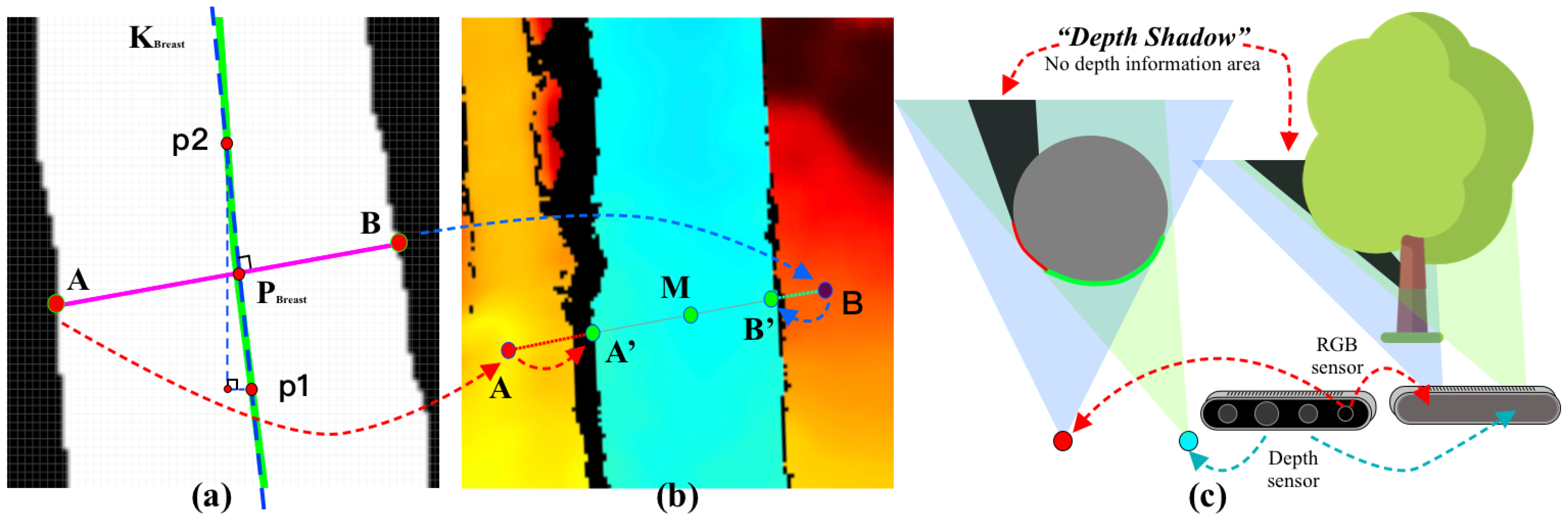
First, we enhanced the segmentation head of the YOLOv5-seg model, incorporating attention mechanisms to more comprehensively capture the global contextual information of tree features, thereby achieving higher segmentation accuracy in a shorter time. On this basis, we propose a novel image-based keypoint localization method for tree masks, which is able to accurately locate two mask edge points (DBH keypoints) whose connecting lines are perpendicular to the tree growth direction at any height of the tree mask. Subsequently, with the help of RGB-D camera, we map the DBH keypoints to the world coordinate system to obtain the DBH. In order to minimize the measurement errors, we discussed several situations that may lead to deviations in the positioning of the DBH keypoints, such as low-quality skeletons and the phenomenon of deep shadows, and then optimized each case accordingly.

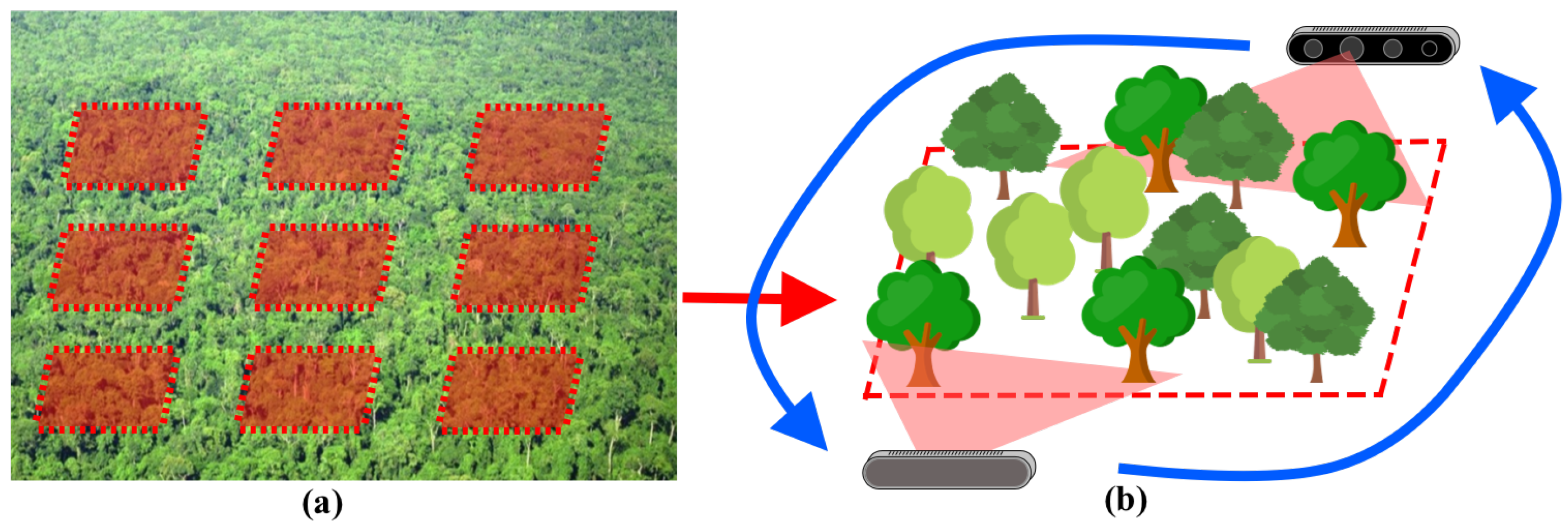
In addition, we designed an optimization method based on target tracking that tracks multiple trees and improves the stability of the algorithm by reducing the probability of outliers during diameter measurements through repeated measurements. We also experimented with a WLAN-based edge computing strategy, and this separated architecture has two major advantages:

• Shifting intensive computational tasks to a remote computing platform not only improves computational efficiency, but also reduces the burden on the low-power devices on the measurement side, allowing them to sample the environment more stably;
• The cost of measurement-side equipment that simplifies the task is dramatically reduced, allowing deployment scales to be equitably increased. More measurement devices are monitored simultaneously at the remote end, improving inventory efficiency.

Accurate tree DBH measurements are important for both traditional forest inventory tasks and vision-based automated path planning for forestry robots. Once our system is activated, the entire process is fully automated, and we have provided a user-friendly graphical interface for operators, providing a solid foundation for future deployment on UAVs, UGVs or UMVs. We look forward to the system playing an even greater role in future unmanned equipment-based forest inventory missions. This will not only move our research forward, but will also revolutionize the entire field of forest resource management by providing more powerful tools to conserve and manage our valuable forest resources.

References

1. Siry, J.P.; Cubbage, F.W.; Ahmed, M.R. Sustainable forest management: Global trends and opportunities. For. Policy Econ. 2005, 7, 551–561. [Google Scholar] [CrossRef]
2. Lindenmayer, D.B.; Margules, C.R.; Botkin, D.B. Indicators of biodiversity for ecologically sustainable forest management. Conserv. Biol. 2000, 14, 941–950. [Google Scholar] [CrossRef]
3. White, J.C.; Coops, N.C.; Wulder, M.A.; Vastaranta, M.; Hilker, T.; Tompalski, P. Remote Sensing Technologies for Enhancing Forest Inventories: A Review. Can. J. Remote Sens. 2016, 42, 619–641. [Google Scholar] [CrossRef]
4. Leverett, B.; Bertolette, D. American Forests Champion Trees Measuring Guidelines Handbook; American Forests: Washington, DC, USA, 2014; Available online: https://www.americanforests.org/wp-content/uploads/2014/12/AF-Tree-Measuring-Guidelines_LR.pdf (accessed on 4 January 2023).
5. Ganz, S.; Käber, Y.; Adler, P. Measuring tree height with remote sensing—A comparison of photogrammetric and LiDAR data with different field measurements. Forests 2019, 10, 694. [Google Scholar] [CrossRef]
6. Larjavaara, M.; Muller-Landau, H.C. Measuring tree height: A quantitative comparison of two common field methods in a moist tropical forest. Methods Ecol. Evol. 2013, 4, 793–801. [Google Scholar] [CrossRef]
7. Krisanski, S.; Taskhiri, M.S.; Turner, P. Enhancing methods for under-canopy unmanned aircraft system based photogrammetry in complex forests for tree diameter measurement. Remote Sens. 2020, 12, 1652. [Google Scholar] [CrossRef]
8. Zhang, Y.; Yang, J.; Li, G.; Zhao, T.; Song, X.; Zhang, S.; Li, A.; Bian, H.; Li, J.; Zhang, M.; et al. Camera calibration for long-distance photogrammetry using unmanned aerial vehicles. J. Sens. 2022, 2022, 8573315. [Google Scholar] [CrossRef]
9. Jiang, R.; Lin, J.; Li, T. Refined Aboveground Biomass Estimation of Moso Bamboo Forest Using Culm Lengths Extracted from TLS Point Cloud. Remote Sens. 2022, 14, 5537. [Google Scholar] [CrossRef]
10. Qiu, Z.; Feng, Z.; Jiang, J.; Lin, Y.; Xue, S. Application of a continuous terrestrial photogrammetric measurement system for plot monitoring in the Beijing Songshan national nature reserve. Remote Sens. 2018, 10, 1080. [Google Scholar] [CrossRef]
11. Peterson, B.; Dubayah, R.; Hyde, P.; Hofton, M.; Blair, J.B.; Fites-Kaufman, J. Use of LIDAR for forest inventory and forest management application. In Proceedings of the Seventh Annual Forest Inventory and Analysis Symposium, Portland, ME, USA, 3–6 October 2005; General Technical Report WO-77. McRoberts, R.E., Reams, G.A., Van Deusen, P.C., McWilliams, W.H., Eds.; US Department of Agriculture, Forest Service: Washington, DC, USA, 2007; Volume 77, pp. 193–202. [Google Scholar]
12. Iglhaut, J.; Cabo, C.; Puliti, S.; Piermattei, L.; O’Connor, J.; Rosette, J. Structure from motion photogrammetry in forestry: A review. Curr. For. Rep. 2019, 5, 155–168. [Google Scholar] [CrossRef]
13. Gollob, C.; Ritter, T.; Kraßnitzer, R.; Tockner, A.; Nothdurft, A. Measurement of forest inventory parameters with Apple iPad pro and integrated LiDAR technology. Remote Sens. 2021, 13, 3129. [Google Scholar] [CrossRef]
14. Wang, Q.; Zhang, Q. Three-dimensional reconstruction of a dormant tree using rgb-d cameras. In Proceedings of the 2013 ASABE Annual International Meeting, Kansas City, MO, USA, 21–24 July 2013; American Society of Agricultural and Biological Engineers: St. Joseph, MI, USA, 2013; p. 1. [Google Scholar]
15. Moosmann, F.; Pink, O.; Stiller, C. Segmentation of 3D lidar data in non-flat urban environments using a local convexity criterion. In Proceedings of the 2009 IEEE Intelligent Vehicles Symposium, Xi’an, China, 3–5 June 2009; pp. 215–220. [Google Scholar]
16. Panagiotidis, D.; Surovỳ, P.; Kuželka, K. Accuracy of Structure from Motion models in comparison with terrestrial laser scanner for the analysis of DBH and height influence on error behaviour. J. For. Sci. 2016, 62, 357–365. [Google Scholar] [CrossRef]
17. Srinivasan, S.; Popescu, S.C.; Eriksson, M.; Sheridan, R.D.; Ku, N.W. Terrestrial laser scanning as an effective tool to retrieve tree level height, crown width, and stem diameter. Remote Sens. 2015, 7, 1877–1896. [Google Scholar] [CrossRef]
18. Brede, B.; Lau, A.; Bartholomeus, H.M.; Kooistra, L. Comparing RIEGL RiCOPTER UAV LiDAR derived canopy height and DBH with terrestrial LiDAR. Sensors 2017, 17, 2371. [Google Scholar] [CrossRef] [PubMed]
19. Wieser, M.; Mandlburger, G.; Hollaus, M.; Otepka, J.; Glira, P.; Pfeifer, N. A case study of UAS borne laser scanning for measurement of tree stem diameter. Remote Sens. 2017, 9, 1154. [Google Scholar] [CrossRef]
20. Gao, Q.; Kan, J. Automatic forest DBH measurement based on structure from motion photogrammetry. Remote Sens. 2022, 14, 2064. [Google Scholar] [CrossRef]
21. Piermattei, L.; Karel, W.; Wang, D.; Wieser, M.; Mokroš, M.; Surovỳ, P.; Koreň, M.; Tomaštík, J.; Pfeifer, N.; Hollaus, M. Terrestrial structure from motion photogrammetry for deriving forest inventory data. Remote Sens. 2019, 11, 950. [Google Scholar] [CrossRef]
22. Jodas, D.S.; Brazolin, S.; Yojo, T.; De Lima, R.A.; Velasco, G.D.N.; Machado, A.R.; Papa, J.P. A deep learning-based approach for tree trunk segmentation. In Proceedings of the 2021 34th SIBGRAPI Conference on Graphics, Patterns and Images (SIBGRAPI), Gramado, Brazil, 18–22 October 2021; pp. 370–377. [Google Scholar]
23. Luo, W.; Ma, H.; Yuan, J.; Zhang, L.; Ma, H.; Cai, Z.; Zhou, W. High-Accuracy Filtering of Forest Scenes Based on Full-Waveform LiDAR Data and Hyperspectral Images. Remote Sens. 2023, 15, 3499. [Google Scholar] [CrossRef]
24. Li, F.; Zhu, H.; Luo, Z.; Shen, H.; Li, L. An adaptive surface interpolation filter using cloth simulation and relief amplitude for airborne laser scanning data. Remote Sens. 2021, 13, 2938. [Google Scholar] [CrossRef]
25. Condotta, I.C.; Brown-Brandl, T.M.; Pitla, S.K.; Stinn, J.P.; Silva-Miranda, K.O. Evaluation of low-cost depth cameras for agricultural applications. Comput. Electron. Agric. 2020, 173, 105394. [Google Scholar] [CrossRef]
26. Fu, L.; Gao, F.; Wu, J.; Li, R.; Karkee, M.; Zhang, Q. Application of consumer RGB-D cameras for fruit detection and localization in field: A critical review. Comput. Electron. Agric. 2020, 177, 105687. [Google Scholar] [CrossRef]
27. Fan, Y.; Feng, Z.; Mannan, A.; Khan, T.U.; Shen, C.; Saeed, S. Estimating tree position, diameter at breast height, and tree height in real-time using a mobile phone with RGB-D SLAM. Remote Sens. 2018, 10, 1845. [Google Scholar] [CrossRef]
28. Holcomb, A.; Tong, L.; Keshav, S. Robust Single-Image Tree Diameter Estimation with Mobile Phones. Remote Sens. 2023, 15, 772. [Google Scholar] [CrossRef]
29. Sun, X.; Fang, W.; Gao, C.; Fu, L.; Majeed, Y.; Liu, X.; Gao, F.; Yang, R.; Li, R. Remote estimation of grafted apple tree trunk diameter in modern orchard with RGB and point cloud based on SOLOv2. Comput. Electron. Agric. 2022, 199, 107209. [Google Scholar] [CrossRef]
30. Liu, T.; Kang, H.; Chen, C. ORB-Livox: A real-time dynamic system for fruit detection and localization. Comput. Electron. Agric. 2023, 209, 107834. [Google Scholar] [CrossRef]
31. da Silva, D.Q.; Dos Santos, F.N.; Sousa, A.J.; Filipe, V. Visible and thermal image-based trunk detection with deep learning for forestry mobile robotics. J. Imaging 2021, 7, 176. [Google Scholar] [CrossRef]
32. Grondin, V.; Fortin, J.M.; Pomerleau, F.; Giguère, P. Tree detection and diameter estimation based on deep learning. Forestry 2023, 96, 264–276. [Google Scholar] [CrossRef]
33. Shi, L.; Wang, G.; Mo, L.; Yi, X.; Wu, X.; Wu, P. Automatic Segmentation of Standing Trees from Forest Images Based on Deep Learning. Sensors 2022, 22, 6663. [Google Scholar] [CrossRef]
34. Girshick, R.; Donahue, J.; Darrell, T.; Malik, J. Rich feature hierarchies for accurate object detection and semantic segmentation. In Proceedings of the IEEE Conference on Computer Vision and Pattern Recognition, Columbus, OH, USA, 23–28 June 2014; pp. 580–587. [Google Scholar]
35. Ren, S.; He, K.; Girshick, R.; Sun, J. Faster r-cnn: Towards real-time object detection with region proposal networks. Adv. Neural Inf. Process. Syst. 2015, 28, 91–99. [Google Scholar] [CrossRef]
36. He, K.; Gkioxari, G.; Dollár, P.; Girshick, R. Mask r-cnn. In Proceedings of the IEEE International Conference on Computer Vision, Venice, Italy, 22–29 October 2017; pp. 2961–2969. [Google Scholar]
37. Redmon, J.; Divvala, S.; Girshick, R.; Farhadi, A. You only look once: Unified, real-time object detection. In Proceedings of the IEEE Conference on Computer Vision and Pattern Recognition, Las Vegas, NV, USA, 27–30 June 2016; pp. 779–788. [Google Scholar]
38. Bolya, D.; Zhou, C.; Xiao, F.; Lee, Y.J. Yolact: Real-time instance segmentation. In Proceedings of the IEEE/CVF International Conference on Computer Vision, Seoul, Republic of Korea, 27 October–2 November 2019; pp. 9157–9166. [Google Scholar]
39. Long, J.; Shelhamer, E.; Darrell, T. Fully convolutional networks for semantic segmentation. In Proceedings of the IEEE Conference on Computer Vision and Pattern Recognition, Boston, MA, USA, 7–12 June 2015; pp. 3431–3440. [Google Scholar]
40. Neubeck, A.; Van Gool, L. Efficient non-maximum suppression. In Proceedings of the 18th International Conference on Pattern Recognition (ICPR’06), Hong Kong, China, 20–24 August 2006; Volume 3, pp. 850–855. [Google Scholar]
41. Cao, L.; Zheng, X.; Fang, L. The Semantic Segmentation of Standing Tree Images Based on the Yolo V7 Deep Learning Algorithm. Electronics 2023, 12, 929. [Google Scholar] [CrossRef]
42. Grondin, V.; Pomerleau, F.; Giguère, P. Training Deep Learning Algorithms on Synthetic Forest Images for Tree Detection. arXiv 2022, arXiv:2210.04104. [Google Scholar]
43. Zhang, T.Y.; Suen, C.Y. A fast parallel algorithm for thinning digital patterns. Commun. ACM 1984, 27, 236–239. [Google Scholar] [CrossRef]
44. Danciu, G.; Banu, S.M.; Căliman, A. Shadow removal in depth images morphology-based for Kinect cameras. In Proceedings of the 2012 16th International Conference on System Theory, Control and Computing (ICSTCC), Sinaia, Romania, 12–14 October 2012; pp. 1–6. [Google Scholar]
45. Wang, W.; Dai, J.; Chen, Z.; Huang, Z.; Li, Z.; Zhu, X.; Hu, X.; Lu, T.; Lu, L.; Li, H.; et al. Internimage: Exploring large-scale vision foundation models with deformable convolutions. In Proceedings of the IEEE/CVF Conference on Computer Vision and Pattern Recognition, Vancouver, BC, Canada, 18–22 June 2023; pp. 14408–14419. [Google Scholar]
46. Han, X.L.; Jiang, N.J.; Yang, Y.F.; Choi, J.; Singh, D.N.; Beta, P.; Du, Y.J.; Wang, Y.J. Deep learning based approach for the instance segmentation of clayey soil desiccation cracks. Comput. Geotech. 2022, 146, 104733. [Google Scholar] [CrossRef]
Figure 1. Pipeline of the system.
Forests 14 02334 g001
Figure 2. Schematic of the actual view of the sampling site, with the left subplot showing the geographic location of the experiment. (a) Changchun: Jingyuetan National Forest Park. (b) Beijing: Olympic Forest Park. (c) Beijing: Jiufeng National Forest Park.
Forests 14 02334 g002
Figure 3. Five data enhancement algorithms were chosen: random noise (Salt and Pepper, Gaussian Noise, Gaussian Blue), flipping (Horizontal and Vertical Flip), geometric transformations (Affine Transform, Random Scaling, Random Translation), Random Contrast (Gamma Contrast, Linear Contrast, Random Luminance, Random Saturation), and SnowFlakes.
Forests 14 02334 g003
Figure 4. The components of proposed vision measurement system.
Forests 14 02334 g004
Figure 5. Schematic of sampling strategy. (a) Grid sampling. (b) Concentric circle stepping.
Forests 14 02334 g005
Figure 6. The structure of the YOLOv5-seg model.
Forests 14 02334 g006
Figure 7. The structure of the CBAM module.
Forests 14 02334 g007
Figure 8. The improved segment head of the YOLOv5-seg model.
Forests 14 02334 g008
Figure 9. (a) K B r e a s t is the slope at P B r e a s t , and A and B are the two initially identified points for chest diameter measurement; (b) points A and B may not be accurately mapped in the depth image, and so were progressively adjusted to the position of A′ and B′; (c) an illustration of the reasons for the formation of the depth shadow.
Forests 14 02334 g009
Figure 10. (a) A schematic of the pixel coordinate system mapped to the world coordinate system; (b) the tilted cylinder is a schematic of a tree, where the gray ellipse is a horizontal cross-section of the tree, the green cross-section represents a cross-section that is perpendicular to the skeleton line in space, and the red cross-section represents a non-perpendicular cross-section (the one that is initially looked for), and n is a localized direction vector of the skeleton; (c) three-point fitting circle in the plane.
Forests 14 02334 g010
Figure 11. The segmentation result of the improved YOLOv5nano-seg model.
Forests 14 02334 g011
Figure 12. Comparison of predicted and manual measurement values of DBH in plots.
Forests 14 02334 g012
Figure 13. Boxplot illustrating the error distribution from plots and total.
Forests 14 02334 g013
Figure 14. Instance segmentation results of various sizes: original and proposed model. The first row represents the ground truth annotations; the second row illustrates the results obtained using the original model; the third row shows the better results achieved after improvement. In this analysis, the yellow circle indicates an irregular, slender tree trunk, while the blue circle delineates the tree root segmentation. The green circle highlights mis-segmented tree root sections. It is evident from the figure that enlarging the model size enhances the region of interest (ROI) for segmentation but also notably amplifies mis-segmentation. However, following our enhancements, there is a marked improvement in the model’s segmentation accuracy and its proficiency in identifying correct segmentation content.
Forests 14 02334 g014
Figure 15. The program’s live screen displays depth frames and RGB frames on both sides. Both frames automatically highlight the breast position with an auxiliary line to indicate the measurement location. The top left area provides details such as tree number, radius, and key points’ distances. A line from the center of the tree to the camera helps find the tree quickly. The enlarged image in the center is a detail of a depth map, and is meant to illustrate that all three of the keypoints we located are in the exact position. The red dot in the center is M w , while the white dots on either side are: A w and B w .
Forests 14 02334 g015