
Combining Multisource Data and Machine Learning Approaches for Multiscale Estimation of Forest Biomass

 , ,
, ,
Abstract
:1. Introduction
2. Materials and Methods
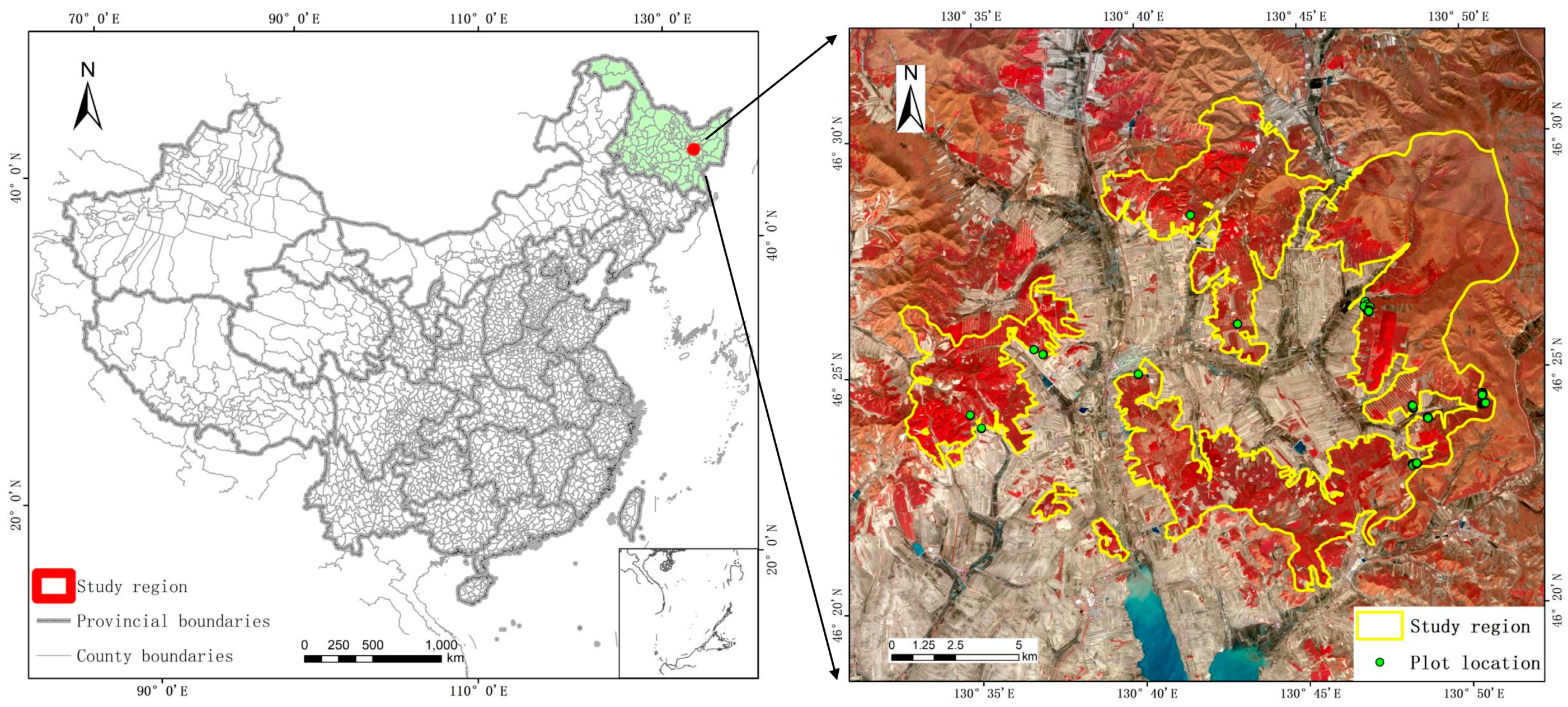
2.1. Study Area
2.2. Data
2.2.1. Field Data
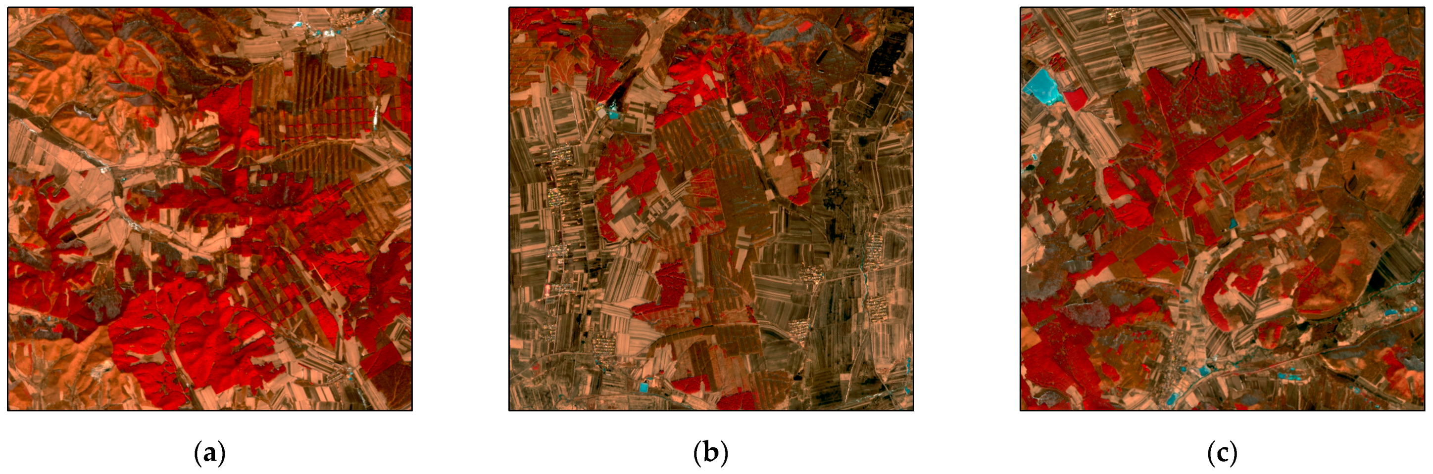
2.2.2. Remotely Sensed Data
- (1)
- LiDAR Data
- (2)
- Optical Data
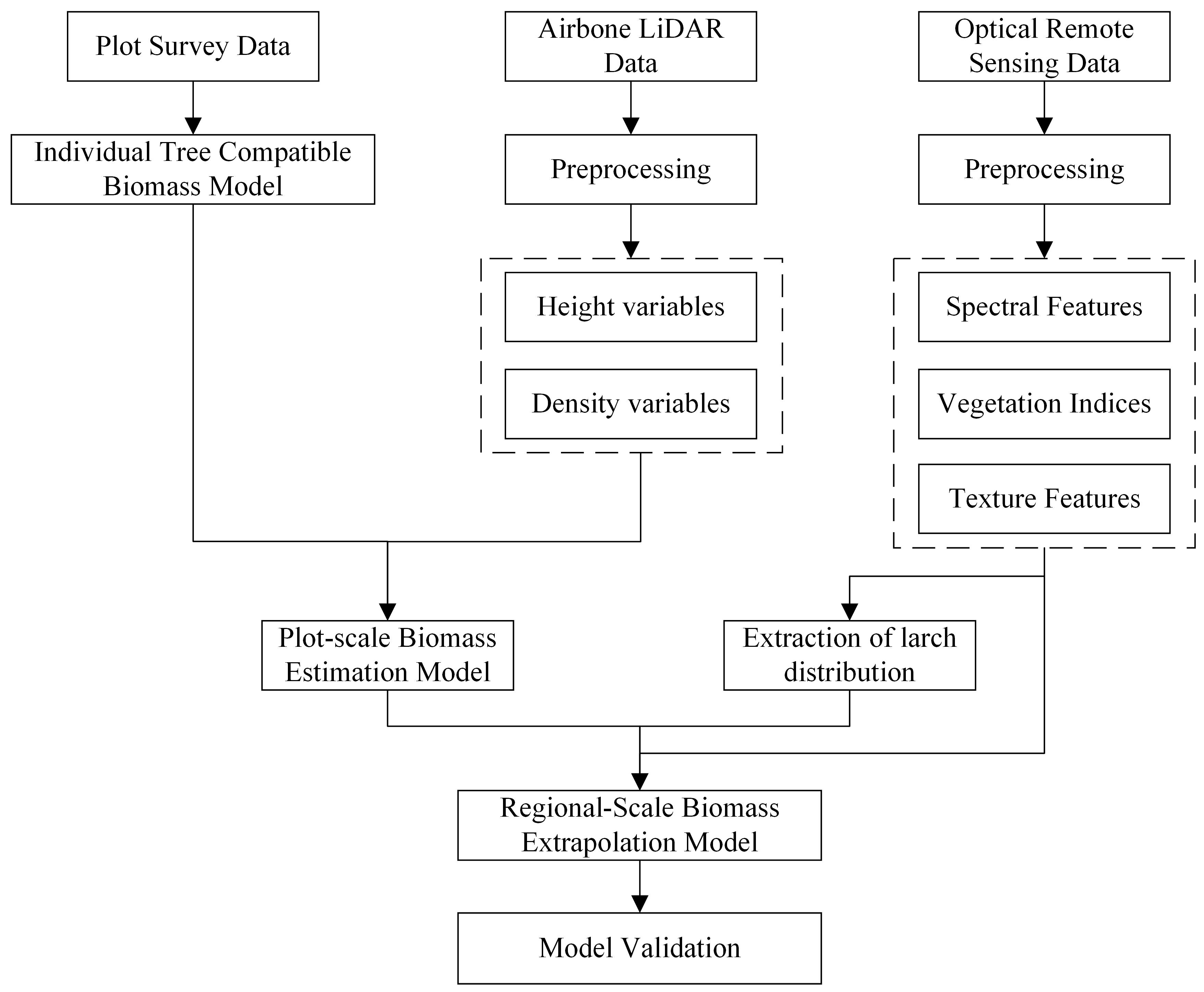
2.3. Methods
2.3.1. Build a Basic Model of Larch Biomass Compatibility
2.3.2. Build a Plot-Scale Biomass Component Estimation Model on the Basis of Airborne LiDAR Data
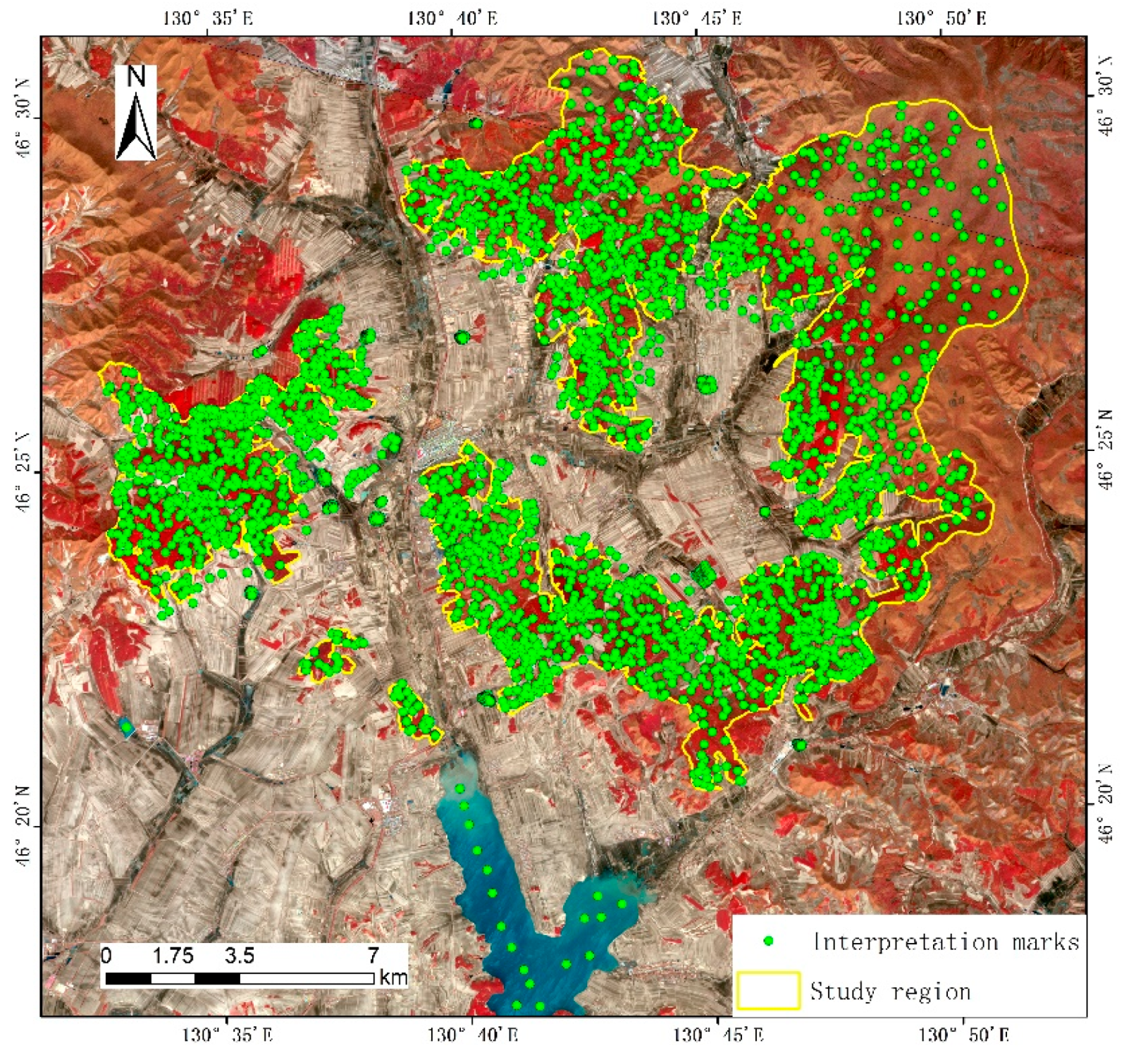
2.3.3. Extraction of Larch Distribution Information on the Basis of Vegetation Phenology Characteristics
2.3.4. Construction of a Model for Extrapolation of Biomass Components at the Regional Scale
2.3.5. Model Evaluation
3. Results
3.1. Basic Model of Larch Biomass Compatibility
3.2. Plot-Scale Biomass Component Estimation Model Based on Airborne LiDAR Data
3.3. Extraction of Larch Distribution Information Based on Vegetation Phenology Characteristics
3.4. Construction of a Regional-Scale Biomass Component Extrapolation Model Based on Multisource Data Fusion
4. Discussion
4.1. Performance of Regression-Based Method and Machine Learning Algorithms
4.2. Extraction of Larch Distribution Information
4.3. Extrapolation Model of Biomass Components
4.4. Trade-Off between the Accuracy and Cost in Biomass Estimation
5. Conclusions
Author Contributions
Funding
Data Availability Statement
Conflicts of Interest
Glossary
| Abbreviation | Definition | Units |
| LSTM | Long short-term memory | |
| DBH | Diameter at breast height | cm |
| H | Height of a tree | m |
| Hi | Altitude percentiles extracted from LiDAR points | |
| AIHi | Cumulative altitude percentiles extracted from LiDAR points | |
| Di | Density variable extracted from LiDAR points | |
| GF-1 | Gaofen-1 satellite | |
| PMS1 | One of high-resolution cameras on the GF-1 | |
| MLR | Multiple linear regression | |
| RF | Random forest | |
| SVM | Support vector machine | |
| Kappa | Kappa coefficient, an indicator to evaluate the accuracy of classification | |
| RNN | Recurrent neural network | |
| Coefficient of determination | ||
| Adjusting coefficient of determination | ||
| RMSE | Root mean square error | |
| rRMSE | Relative root mean square error | |
| SEE | Standard deviation of the estimated value | |
| TRE | Total relative error | |
| MPE | Mean estimation error | |
| MSE | Mean systematic error | |
| MPSE | Mean percentage standard error | |
| a | The fitting parameter in biomass model | |
| b | The fitting parameter in biomass model | |
| B | Biomass | ton |
| BStem | Biomass of stem | ton |
| BBark | Biomass of bark | ton |
| BBranch | Biomass of branch | ton |
| BLeaf | Biomass of leaf | ton |
| BRoot | Biomass of root | ton |
| BAbove | Aboveground biomass | ton |
| BTotal | Total biomass | ton |
| t | Ton | ton |
References
- Zeng, W.; Xiao, Q.; Hu, J.; Liao, Z. Establishment of single-tree biomass equations for Pinus massoniana in southern China. J. Cent. South Univ. Technol. 2010, 30, 50–56. [Google Scholar]
- Myneni, R.B.; Dong, J.; Tucker, C.J.; Kaufmann, R.K.; Kauppi, P.E.; Liski, J.; Zhou, L.; Alexeyev, V.; Hughes, M. A large carbon sink in the woody biomass of Northern forests. Proc. Natl. Acad. Sci. USA 2001, 98, 14784–14789. [Google Scholar] [CrossRef]
- Yu, G.; Fang, H.; Fu, Y.; Wang, Q. Research on carbon budget and carbon cycle of terrestrial ecosystems in regional scale: A review. Shengtai Xuebao/Acta Ecol. Sin. 2011, 31, 5449–5459. [Google Scholar]
- Awad, M.M. FlexibleNet: A New Lightweight Convolutional Neural Network Model for Estimating Carbon Sequestration Qualitatively Using Remote Sensing. Remote Sens. 2023, 15, 272. [Google Scholar] [CrossRef]
- Nishizono, T.; Iehara, T.; Kuboyama, H.; Fukuda, M. A forest biomass yield table based on an empirical model. J. For. Res. 2005, 10, 211–220. [Google Scholar] [CrossRef]
- Yu, Q.; Wang, Y.; Van Le, Q.; Yang, H.; Hosseinzadeh-Bandbafha, H.; Yang, Y.; Sonne, C.; Tabatabaei, M.; Lam, S.S.; Peng, W. An overview on the conversion of forest biomass into bioenergy. Front. Energy Res. 2021, 9, 684234. [Google Scholar] [CrossRef]
- Herold, M.; Carter, S.; Avitabile, V.; Espejo, A.B.; Jonckheere, I.; Lucas, R.; McRoberts, R.E.; Næsset, E.; Nightingale, J.; Petersen, R. The role and need for space-based forest biomass-related measurements in environmental management and policy. Surv. Geophys. 2019, 40, 757–778. [Google Scholar] [CrossRef]
- Tang, X.; Zhao, X.; Bai, Y.; Tang, Z.; Wang, W.; Zhao, Y.; Wan, H.; Xie, Z.; Shi, X.; Wu, B. Carbon pools in China’s terrestrial ecosystems: New estimates based on an intensive field survey. Proc. Natl. Acad. Sci. USA 2018, 115, 4021–4026. [Google Scholar] [CrossRef]
- Zhou, G.; Meng, C.; Jiang, P.; Xu, Q. Review of carbon fixation in bamboo forests in China. Bot. Rev. 2011, 77, 262–270. [Google Scholar] [CrossRef]
- Lambert, M.; Ung, C.; Raulier, F. Canadian national tree aboveground biomass equations. Can. J. For. Res. 2005, 35, 1996–2018. [Google Scholar] [CrossRef]
- Shen, Y.; Sun, X.; Zhang, J.; Ma, J. Study on the individual tree biomass of Larix kaempferi plantation in Xiaolong Mountain, Gansu Province. For. Res. 2011, 24, 517–522. [Google Scholar]
- Fu, L.; Zeng, W.; Tang, S.; Sharma, R.; Li, H. Using linear mixed model and dummy variable model approaches to construct compatible single-tree biomass equations at different scales-A case study for Masson pine in Southern China. J. For. Sci. 2012, 58, 101–115. [Google Scholar] [CrossRef]
- Haara, A.; Leskinen, P. The assessment of the uncertainty of updated stand-level inventory data. Silva Fenn. 2009, 43, 87–112. [Google Scholar] [CrossRef]
- Lei, X.; Yu, L.; Hong, L. Climate-sensitive integrated stand growth model (CS-ISGM) of Changbai larch (Larix olgensis) plantations. For. Ecol. Manag. 2016, 376, 265–275. [Google Scholar] [CrossRef]
- Zhang, Y.; Liang, S.; Yang, L. A review of regional and global gridded forest biomass datasets. Remote Sens. 2019, 11, 2744. [Google Scholar] [CrossRef]
- Wigneron, J.-P.; Li, X.; Frappart, F.; Fan, L.; Al-Yaari, A.; De Lannoy, G.; Liu, X.; Wang, M.; Le Masson, E.; Moisy, C. SMOS-IC data record of soil moisture and L-VOD: Historical development, applications and perspectives. Remote Sens. Environ. 2021, 254, 112238. [Google Scholar] [CrossRef]
- Tong, X.; Brandt, M.; Yue, Y.; Ciais, P.; Rudbeck Jepsen, M.; Penuelas, J.; Wigneron, J.-P.; Xiao, X.; Song, X.-P.; Horion, S. Forest management in southern China generates short term extensive carbon sequestration. Nat. Commun. 2020, 11, 129. [Google Scholar] [CrossRef]
- Fayad, I.; Baghdadi, N.; Guitet, S.; Bailly, J.-S.; Hérault, B.; Gond, V.; El Hajj, M.; Minh, D.H.T. Aboveground biomass mapping in French Guiana by combining remote sensing, forest inventories and environmental data. Int. J. Appl. Earth Obs. Geoinf. 2016, 52, 502–514. [Google Scholar] [CrossRef]
- Cao, Q.; Xu, D.; Ju, H. Biomass estimation of five kinds of mangrove community with the KNN method based on the spectral information and textural features of TM images. For. Res. 2011, 24, 144–150. [Google Scholar]
- El Hajj, M.; Baghdadi, N.; Labrière, N.; Bailly, J.-S.; Villard, L. Mapping of aboveground biomass in Gabon. Comptes Rendus Géosci. 2019, 351, 321–331. [Google Scholar] [CrossRef]
- Guo, Q.; Su, Y.; Hu, T.; Guan, H.; Jin, S.; Zhang, J.; Zhao, X.; Xu, K.; Wei, D.; Kelly, M. Lidar boosts 3D ecological observations and modelings: A review and perspective. IEEE Geosci. Remote Sens. Mag. 2020, 9, 232–257. [Google Scholar] [CrossRef]
- Liu, Q.; Li, Z.; Chen, E.; Pang, Y.; Tian, X.; Cao, C. Estimating biomass of individual trees using point cloud data of airborne LIDAR. High Technol. Lett. 2010, 20, 765–770. [Google Scholar]
- Næsset, E.; Gobakken, T. Estimation of above- and below-ground biomass across regions of the boreal forest zone using airborne laser. Remote Sens. Environ. 2008, 112, 3079–3090. [Google Scholar] [CrossRef]
- Mougin, E.; Proisy, C.; Marty, G.; Fromard, F.; Puig, H.; Betoulle, J.; Rudant, J.-P. Multifrequency and multipolarization radar backscattering from mangrove forests. IEEE Trans. Geosci. Remote Sens. 1999, 37, 94–102. [Google Scholar] [CrossRef]
- Qiu, S.; Xing, Y.; Xu, W. Estimation of regional forest aboveground biomass combining spaceborne large footprint LiDAR and HJ-1A hyperspectral images. Acta Ecol. Sin. 2016, 36, 7401–7411. [Google Scholar]
- Tolan, J.; Yang, H.-I.; Nosarzewski, B.; Couairon, G.; Vo, H.; Brandt, J.; Spore, J.; Majumdar, S.; Haziza, D.; Vamaraju, J. Sub-meter resolution canopy height maps using self-supervised learning and a vision transformer trained on Aerial and GEDI Lidar. arXiv 2023, arXiv:2304.07213. [Google Scholar]
- Wagner, F.H.; Roberts, S.; Ritz, A.L.; Carter, G.; Dalagnol, R.; Favrichon, S.; Hirye, M.; Brandt, M.; Ciais, P.; Saatchi, S. Sub-Meter Tree Height Mapping of California using Aerial Images and LiDAR-Informed U-Net Model. arXiv 2023, arXiv:2306.01936. [Google Scholar]
- Yang, S.; Zhang, K.; Shao, Y. Classification of Airborne LiDAR Point Cloud Data Based on Multiscale Adaptive Features. Acta Opt. Sin. 2019, 39, 0228001. [Google Scholar] [CrossRef]
- Fan, S.; Zhang, A.; Hu, S.; Sun, W. A method of classification for airborne full waveform LiDAR data based on random forest. Chin. J. Lasers 2013, 40, 0914001. [Google Scholar]
- Shu, Z.; Sun, K.; Qiu, K.; Ding, K. Pairwise-Svm for On-Board Urban Road LIDAR Classification. Int. Arch. Photogramm. Remote Sens. Spat. Inf. Sci. 2016, 41, 109. [Google Scholar] [CrossRef]
- Ma, H.; Gao, X.; Gu, X. Random forest classification of Landsat 8 imagery for the complex terrain area based on the combination of spectral, topographic and texture information. J. Geo-Inf. Sci. 2019, 21, 359–371. [Google Scholar]
- Dube, T.; Mutanga, O. Evaluating the utility of the medium-spatial resolution Landsat 8 multispectral sensor in quantifying aboveground biomass in uMgeni catchment, South Africa. ISPRS J. Photogramm. Remote Sens. 2015, 101, 36–46. [Google Scholar] [CrossRef]
- Kajisa, T.; Murakami, T.; Mizoue, N.; Top, N.; Yoshida, S. Object-based forest biomass estimation using Landsat ETM+ in Kampong Thom Province, Cambodia. J. For. Res. 2009, 14, 203–211. [Google Scholar] [CrossRef]
- Foody, G.M.; Boyd, D.S.; Cutler, M.E. Predictive relations of tropical forest biomass from Landsat TM data and their transferability between regions. Remote Sens. Environ. 2003, 85, 463–474. [Google Scholar] [CrossRef]
- Wang, L.-H.; Xing, Y.-Q. Remote sensing estimation of natural forest biomass based on an artificial neural network. Ying Yong Sheng Tai Xue Bao J. Appl. Ecol. 2008, 19, 261–266. [Google Scholar]
- Mountrakis, G.; Im, J.; Ogole, C. Support vector machines in remote sensing: A review. ISPRS J. Photogramm. Remote Sens. 2011, 66, 247–259. [Google Scholar] [CrossRef]
- Sun, F.; Yuan, J.; Lu, S. The change and test of climate in Northeast China over the last 100 years. Clim. Environ. Res. 2006, 11, 101–108. [Google Scholar]
- Wang, X.-Y.; Zhao, C.-Y.; Jia, Q.-Y. Impacts of climate change on forest ecosystems in Northeast China. Adv. Clim. Chang. Res. 2013, 4, 230–241. [Google Scholar]
- Husch, B.; Beers, T.W.; Kershaw, J.A., Jr. Forest Mensuration; John Wiley & Sons: Hoboken, NJ, USA, 2002. [Google Scholar]
- Xuan, Z.; Zhang, Q.; Ge, L.; He, H.; Xu, M.; Xu, W. Biomass structure and distribution of Korean Larch Plantations. For. Resour. Manag. 2013, 1, 53. [Google Scholar]
- Mo, D.; Wu, Q.; Lin, N.; Zhuo, Y. Carbon and nitrogen storage and their allocation pattern in Cryptomeria fortunei plantations in southeastern Guangxi of South China. Chin. J. Ecol. 2012, 1, 794–799. [Google Scholar]
- Yan, S.; Gao, R.; Chen, G.; Zhang, R. Carbon Stock and Carbon Sequestration of Successive Planting Chinese Fir in Different Rotations. J.-Northeast. For. Univ. Chin. Ed. 2006, 34, 42. [Google Scholar]
- Pang, Y.; Li, Z.; Ju, H.; Lu, H.; Jia, W.; Si, L.; Guo, Y.; Liu, Q.; Li, S.; Liu, L. LiCHy: The CAF’s LiDAR, CCD and hyperspectral integrated airborne observation system. Remote Sens. 2016, 8, 398. [Google Scholar] [CrossRef]
- Zhao, X.; Guo, Q.; Su, Y.; Xue, B. Improved progressive TIN densification filtering algorithm for airborne LiDAR data in forested areas. ISPRS J. Photogramm. Remote Sens. 2016, 117, 79–91. [Google Scholar] [CrossRef]
- Li, Z.; Liu, Q.; Pang, Y. Review on forest parameters inversion using LiDAR. J. Remote Sens. 2016, 20, 1138–1150. [Google Scholar]
- Dong, L.; Li, F. Additive stand-level biomass models for natural larch forest in the east of Daxing’an mountains. Sci. Silvae Sin. 2016, 52, 13–20. [Google Scholar]
- Fu, L.; Lei, Y.; Sun, W.; Tang, S.; Zeng, W. Development of compatible biomass models for trees from different stand origin. Acta Ecol. Sin. 2014, 34, 1461–1470. [Google Scholar]
- Parresol, B.R. Additivity of nonlinear biomass equations. Can. J. For. Res. 2001, 31, 865–878. [Google Scholar] [CrossRef]
- Hong, Y.; Chen, D.; Shen, J.; Sun, X.; Zhang, S. Compatible biomass models for Larix olgensis plantation based on tree-level and stand-level. For. Res. 2019, 32, 33–40. [Google Scholar]
- Hong, Y.; Zhang, S.; Chen, W.; Chen, D.; Xiang, W.; Pang, Y. Inversion of Biomass Components for Larix olgensis Plantation Using Airborne LiDAR. For. Res. 2019, 32, 83–90. [Google Scholar]
- Li, M.; Kang, X.; Fan, W. Burned area extraction in Huzhong forests based on remote sensing and the spatial analysis of the burned severity. Sci. Silvae Sin. 2017, 53, 163–174. [Google Scholar]
- Wang, X.; Chen, E.; Li, Z.; Yao, W.; Zhao, L. Multi-temporal and dual-polarization SAR for forest land type classification. Sci. Silvae Sin. 2014, 50, 83–91. [Google Scholar]
- Xing, Z.; Li, Y.; Deng, R.; Zhu, H.; Fu, B. Extracting farmland shelterbelt automatically based on ZY-3 remote sensing images. Sci. Silvae Sin. 2016, 52, 11–20. [Google Scholar]
- Giles, C.L.; Kuhn, G.M.; Williams, R.J. Dynamic recurrent neural networks: Theory and applications. IEEE Trans. Neural Netw. 1994, 5, 153–156. [Google Scholar] [CrossRef]
- Schuster, M.; Paliwal, K.K. Bidirectional recurrent neural networks. IEEE Trans. Signal Process. 1997, 45, 2673–2681. [Google Scholar] [CrossRef]
- Hochreiter, S.; Schmidhuber, J. Long short-term memory. Neural Comput. 1997, 9, 1735–1780. [Google Scholar] [CrossRef]
- Schumann, O.; Wöhler, C.; Hahn, M.; Dickmann, J. Comparison of random forest and long short-term memory network performances in classification tasks using radar. In Proceedings of the 2017 Sensor Data Fusion: Trends, Solutions, Applications (SDF), Bonn, Germany, 10–12 October 2017; pp. 1–6. [Google Scholar]
- Van Houdt, G.; Mosquera, C.; Nápoles, G. A review on the long short-term memory model. Artif. Intell. Rev. 2020, 53, 5929–5955. [Google Scholar] [CrossRef]
- Kinga, D.A. A method for stochastic optimization. In Proceedings of the International Conference on Learning Representations, ICLR 2015, San Diego, CA, USA, 7–9 May 2015. [Google Scholar]
- Li, G.; Xie, Z.; Jiang, X.; Lu, D.; Chen, E. Integration of ZiYuan-3 multispectral and stereo data for modeling aboveground biomass of larch plantations in North China. Remote Sens. 2019, 11, 2328. [Google Scholar] [CrossRef]
- Talucci, A.C.; Forbath, E.; Kropp, H.; Alexander, H.D.; DeMarco, J.; Paulson, A.K.; Zimov, N.S.; Zimov, S.; Loranty, M.M. Evaluating post-fire vegetation recovery in Cajander Larch Forests in Northeastern Siberia using UAV derived vegetation indices. Remote Sens. 2020, 12, 2970. [Google Scholar] [CrossRef]
- Naik, P.; Dalponte, M.; Bruzzone, L. Prediction of forest aboveground biomass using multitemporal multispectral remote sensing data. Remote Sens. 2021, 13, 1282. [Google Scholar] [CrossRef]
- Pang, Y.; Li, Z.-Y. Inversion of biomass components of the temperate forest using airborne Lidar technology in Xiaoxing’an Mountains, Northeastern of China. Chin. J. Plant Ecol. 2012, 36, 1095. [Google Scholar] [CrossRef]
- Yang, J.; Huang, X. The 30 m annual land cover dataset and its dynamics in China from 1990 to 2019. Earth Syst. Sci. Data 2021, 13, 3907–3925. [Google Scholar] [CrossRef]
- Zhao, Y.; Zeng, Y.; Zheng, Z.; Dong, W.; Zhao, D.; Wu, B.; Zhao, Q. Forest species diversity mapping using airborne LiDAR and hyperspectral data in a subtropical forest in China. Remote Sens. Environ. 2018, 213, 104–114. [Google Scholar] [CrossRef]
- Badhwar, G. Classification of corn and soybeans using multitemporal thematic mapper data. Remote Sens. Environ. 1984, 16, 175–181. [Google Scholar] [CrossRef]
- Conese, C.; Maselli, F. Use of multitemporal information to improve classification performance of TM scenes in complex terrain. ISPRS J. Photogramm. Remote Sens. 1991, 46, 187–197. [Google Scholar] [CrossRef]
- Tian, J.; Xing, Y.; Yao, S.; Zeng, X.; Jiao, Y. Comparison of Landsat-TM image forest type classification based on cellular automata and BP neural network algorithm. Sci. Silvae Sin. 2017, 53, 26–34. [Google Scholar]
- Lo, T.C.; Scarpace, F.L.; Lillesand, T.M. Use of multitemporal spectral profiles in agricultural land-cower classification. Photogramm. Eng. Remote Sens. 1986, 52, 535–544. [Google Scholar]
- Cao, L.; Li, H.; Han, Y.; Yu, F.; Gu, H. Application of convolutional neural networks in classification of high resolution remote sensing imagery. Sci. Surv. Mapp. 2016, 41, 170–175. [Google Scholar]
- Liu, D.; Han, L.; Han, X. High spatial resolution remote sensing image classification based on deep learning. Acta Opt. Sin. 2016, 36, 306–314. [Google Scholar]
- Fu, W.; Zou, W. Review of Remote Sensing Image Classification Based on Deep Learning. Appl. Res. Comput. 2018, 35, 3521–3525. [Google Scholar]
- Zeng, J.; Zhang, X. Laoshan forest biomass estimation based on GF-1 images with inversion algorithm. J. Cent. South Univ. For. Technol. 2016, 36, 46–51. [Google Scholar]
- Liu, F.; Feng, Z.; Zhao, F.; Song, Y. Biomass inversion study of ZY-3 remote sensing satellite imagery. J. Northwest For. Univ. 2015, 30, 175–181. [Google Scholar]
- Huang, X.; Sun, X.; Zhang, S.; Chen, D. Compatible biomass models for Larix kaempferi in mountainous area of eastern Liaoning. For. Res. 2014, 27, 142–148. [Google Scholar]


| Ages | DBH (cm) | H (m) | Basal Area (m2·ha) | Density (Trees·ha) | ||||
|---|---|---|---|---|---|---|---|---|
| Mean | Range | Mean | Range | Mean | Range | Mean | Range | |
| Young stand | 8.6 | 5.6~11.0 | 18.51 | 12.94~26.16 | 21.6 | 16.8~24.7 | 1825 | 1700~1950 |
| Middle-aged stand | 12.7 | 11.8~13.3 | 15.81 | 13.55~24.86 | 25.2 | 23.2~28.7 | 1589 | 1283~1750 |
| Near-mature stand | 17.7 | 16.6~19.5 | 20.27 | 19.28~21.16 | 33.6 | 27.3~49.9 | 1233 | 1050~1467 |
| Mature stand | 22.8 | 16.9~31.5 | 26.82 | 23.85~29.41 | 26.4 | 16.8~33.4 | 672 | 417~1133 |
| Ages | Numbers of Trees | DBH/cm | Height/m | Stem/kg | Bark/kg | Branch/kg | Leaf/kg | Root/kg |
|---|---|---|---|---|---|---|---|---|
| Young stand | 16 | 3.4~9.2 | 3.7~13.8 | 1.7~15.9 | 0.3~2.9 | 0.7~4.8 | 0.6~2.0 | 0.8~5.2 |
| Middle-aged stand | 16 | 9.2~13.1 | 6.5~17.1 | 10.1~48.6 | 2.1~7.1 | 3.7~9.0 | 1.5~3.1 | 4.7~11.9 |
| Near-mature stand | 16 | 12.9~16.7 | 11.3~18.4 | 26.9~106.4 | 4.0~12.3 | 5.4~12.3 | 1.8~3.5 | 7.4~20.1 |
| Mature stand | 16 | 17.2~23.0 | 11.7~20.8 | 64.0~185.7 | 7.9~19.2 | 8.7~19.4 | 2.5~5.6 | 15.8~49.9 |
| Sample NO. | DBH (cm) | Basal Area (m2·ha) | Density (Trees·ha) | |
|---|---|---|---|---|
| Mean | Range | |||
| 1 | 8.85 | 5.3~15.4 | 18.46 | 2850 |
| 2 | 10.63 | 5.5~19.7 | 16.78 | 1783 |
| 3 | 10.29 | 4.8~16.2 | 22.13 | 2517 |
| 4 | 12.53 | 7.0~18.6 | 15.85 | 1233 |
| 5 | 19.19 | 6.5~26.4 | 16.44 | 550 |
| 6 | 16.87 | 9.5~23.4 | 16.25 | 700 |
| 7 | 17.61 | 10.1~25.5 | 18.86 | 750 |
| 8 | 16.64 | 6.5~22.2 | 21.08 | 933 |
| 9 | 17.03 | 5.6~23.5 | 16.38 | 683 |
| 10 | 17.80 | 9.9~26.3 | 15.64 | 600 |
| Satellite/Sensor | Resolution | Date | Orbit Number | Use |
|---|---|---|---|---|
| GF-1/PMS1 | 2 m/8 m | 26 March 16 | E 130.7/N 46.3, E 130.8/N 46.6; | Extraction of L. olgensis distribution information and the construction 171 of the biomass estimation model |
| 6 July 16 | E 130.7/N 46.6, E 130.6/N 46.3 | |||
| 18 September18 | E 129.9/ N45.5 | Evaluation of the biomass estimation model |
| Grayscale Compression Parameters | Sliding Window | Step Size | Direction |
|---|---|---|---|
| 64 levels | 9 × 9 | 1 | 135° |
| Components | Parameter Estimates | Evaluation Statistics | ||||||
|---|---|---|---|---|---|---|---|---|
| a | b | SEE (t) | TRE (%) | MPE (%) | MSE (%) | MPSE (%) | ||
| Stem | 0.06 | 2.51 | 0.97 | 14.59 | 9.03 | 7.03 | 6.31 | 18.47 |
| Bark | 0.03 | 1.99 | 0.95 | 1.78 | 7.70 | 7.21 | 6.52 | 17.34 |
| Branch | 0.16 | 1.46 | 0.92 | 1.69 | 5.91 | 5.40 | 5.98 | 16.81 |
| Leaf | 0.24 | 0.91 | 0.84 | 0.49 | 5.69 | 4.73 | 5.69 | 16.21 |
| Root | 0.04 | 2.10 | 0.96 | 4.20 | 10.85 | 8.01 | 7.50 | 17.15 |
| Aboveground | 0.96 | 18.01 | 8.41 | 6.58 | 6.38 | 16.74 | ||
| Total | 0.96 | 21.02 | 8.80 | 6.44 | 6.53 | 16.38 | ||
| Components | Parameter Estimates | Evaluation Statistics | ||||||
|---|---|---|---|---|---|---|---|---|
| a0 | b1 | b2 | b3 | R2 | RMSE (t) | rRMSE | TRE (%) | |
| Stem | −2.76 ** | −0.63 ** | 1.70 ** | 11.85 ** | 0.91 | 0.41 | 0.08 | 0.60 |
| Bark | −3.12 ** | −0.88 ** | 1.19 ** | 10.78 ** | 0.83 | 0.05 | 0.08 | 0.66 |
| Branch | −0.87 * | −0.79 ** | 0.44 ** | 7.35 * | 0.54 | 0.07 | 0.10 | 0.91 |
| Leaf | 0.11 | −1.10 ** | −0.167 | 5.86 | 0.634 | 0.15 | 0.68 | 0.96 |
| Root | −2.57 ** | −0.60 ** | 1.145 ** | 8.38 ** | 0.87 | 0.08 | 0.067 | 0.45 |
| Aboveground | −1.59 ** | −0.65 ** | 1.40 ** | 10.58 ** | 0.91 | 0.46 | 0.067 | 0.45 |
| Total | −1.30 ** | −0.64 ** | 1.36 ** | 10.22 ** | 0.91 | 0.534 | 0.07 | 0.45 |
| Components | R2 | RMSE (t) | rRMSE | TRE (%) |
|---|---|---|---|---|
| Stem | 0.97 | 0.54 | 0.11 | 1.067 |
| Bark | 0.96 | 0.05 | 0.09 | 0.73 |
| Branch | 0.92 | 0.07 | 0.10 | 0.94 |
| Leaf | 0.91 | 0.03 | 0.14 | 1.94 |
| Root | 0.96 | 0.10 | 0.09 | 0.71 |
| Aboveground | 0.97 | 0.62 | 0.10 | 0.85 |
| Total | 0.97 | 0.72 | 0.09 | 0.81 |
| Classification Types | L. olgensis | Other Coniferous | Broad-Leaved Trees | Cultivated and Unutilized Land | Construction Land | Waters | User Accuracy(%) |
|---|---|---|---|---|---|---|---|
| L. olgensis | 91 | 3 | 1 | 5 | 91.0 | ||
| Other coniferous | 3 | 92 | 2 | 2 | 1 | 92.0 | |
| Broad-leaved trees | 1 | 3 | 88 | 6 | 2 | 88.0 | |
| Cultivated and unutilized land | 1 | 92 | 7 | 92.0 | |||
| Construction land | 1 | 12 | 84 | 3 | 84.0 | ||
| Waters | 4 | 3 | 93 | 93.0 | |||
| Graphic accuracy (%) | 95.8 | 92.9 | 95.7 | 76.0 | 86.6 | 96.9 |
| Components | Evaluation Statistics | |||||||
|---|---|---|---|---|---|---|---|---|
| R2 | RMSE (t) | rRMSE | TRE (%) | |||||
| RF | LSTM | RF | LSTM | RF | LSTM | RF | LSTM | |
| Stem | 0.70 | 0.70 | 0.68 | 0.62 | 0.14 | 0.14 | 1.92 | 1.93 |
| Bark | 0.69 | 0.66 | 0.04 | 0.04 | 0.08 | 0.08 | 0.64 | 0.69 |
| Branch | 0.35 | 0.26 | 0.04 | 0.04 | 0.06 | 0.06 | 0.32 | 0.39 |
| Leaf | 0.50 | 0.44 | 0.02 | 0.02 | 0.10 | 0.11 | 0.92 | 1.11 |
| Root | 0.71 | 0.71 | 0.10 | 0.10 | 0.09 | 0.08 | 0.76 | 0.75 |
| Aboveground | 0.71 | 0.72 | 0.62 | 0.61 | 0.11 | 0.10 | 1.09 | 1.06 |
| Total | 0.71 | 0.71 | 0.74 | 0.72 | 0.11 | 0.10 | 1.08 | 1.04 |
| Models | All Samples | Samples of Biomass > 8 ton | |||
|---|---|---|---|---|---|
| Overestimated | Underestimated | Overestimated | Underestimated | ||
| LSTM | Number of samples | 3758 | 3897 | 512 | 1824 |
| Proportion | 49.1% | 50.9% | 21.9% | 78.1% | |
| RF | Number of samples | 3589 | 4066 | 370 | 1966 |
| Proportion | 46.9% | 53.1% | 15.8% | 84.2% | |
| Components | Evaluation Statistics | |||
|---|---|---|---|---|
| R2 | RMSE (t) | rRMSE | TRE (%) | |
| Stem | 0.53 | 0.31 | 0.11 | 1.01 |
| Bark | 0.45 | 0.04 | 0.09 | 0.71 |
| Branch | 0.08 | 0.11 | 0.19 | 3.31 |
| Leaf | 0.20 | 0.06 | 0.28 | 7.06 |
| Root | 0.50 | 0.06 | 0.08 | 0.58 |
| Aboveground | 0.65 | 0.29 | 0.07 | 0.43 |
| Total | 0.63 | 0.35 | 0.07 | 0.43 |
Disclaimer/Publisher’s Note: The statements, opinions and data contained in all publications are solely those of the individual author(s) and contributor(s) and not of MDPI and/or the editor(s). MDPI and/or the editor(s) disclaim responsibility for any injury to people or property resulting from any ideas, methods, instructions or products referred to in the content. |
© 2023 by the authors. Licensee MDPI, Basel, Switzerland. This article is an open access article distributed under the terms and conditions of the Creative Commons Attribution (CC BY) license (https://creativecommons.org/licenses/by/4.0/).
Share and Cite
Hong, Y.; Xu, J.; Wu, C.; Pang, Y.; Zhang, S.; Chen, D.; Yang, B. Combining Multisource Data and Machine Learning Approaches for Multiscale Estimation of Forest Biomass. Forests 2023, 14, 2248. https://doi.org/10.3390/f14112248
Hong Y, Xu J, Wu C, Pang Y, Zhang S, Chen D, Yang B. Combining Multisource Data and Machine Learning Approaches for Multiscale Estimation of Forest Biomass. Forests. 2023; 14(11):2248. https://doi.org/10.3390/f14112248
Chicago/Turabian StyleHong, Yifeng, Jiaming Xu, Chunyan Wu, Yong Pang, Shougong Zhang, Dongsheng Chen, and Bo Yang. 2023. "Combining Multisource Data and Machine Learning Approaches for Multiscale Estimation of Forest Biomass" Forests 14, no. 11: 2248. https://doi.org/10.3390/f14112248