
Carnivorous Plant Algorithm and BP to Predict Optimum Bonding Strength of Heat-Treated Woods
Abstract
:1. Introduction
2. Methods
2.1. Data Preparation
T-Test and ANOVA
2.2. Prediction Models
2.2.1. Carnivorous Plant Algorithm (CPA)
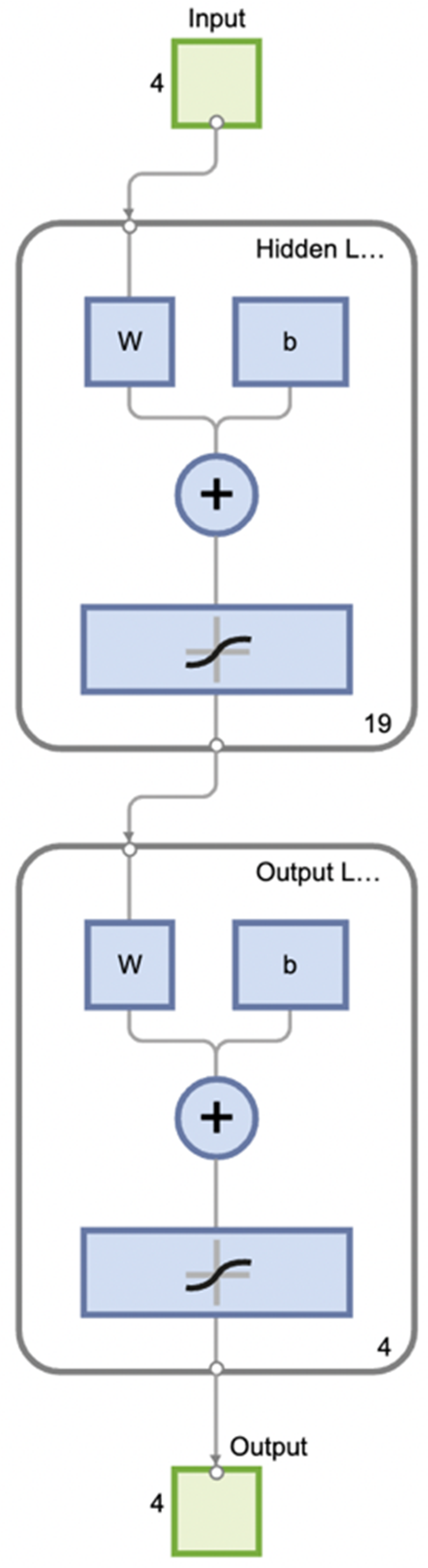
2.2.2. BP Neural Network
2.2.3. Random Forests Algorithm (RF)
2.2.4. Model Performance Evaluation
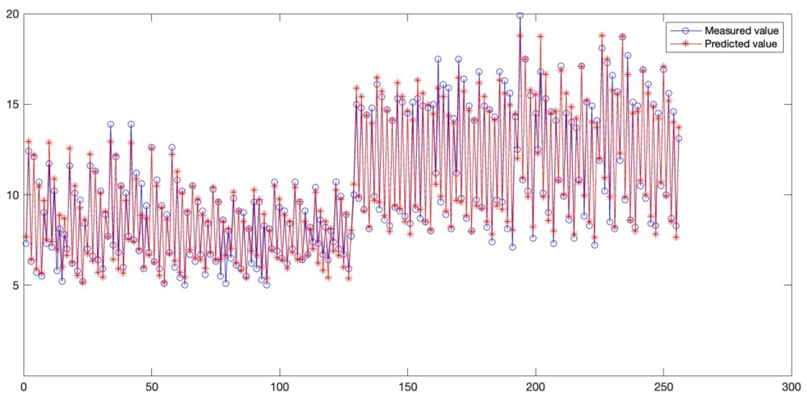
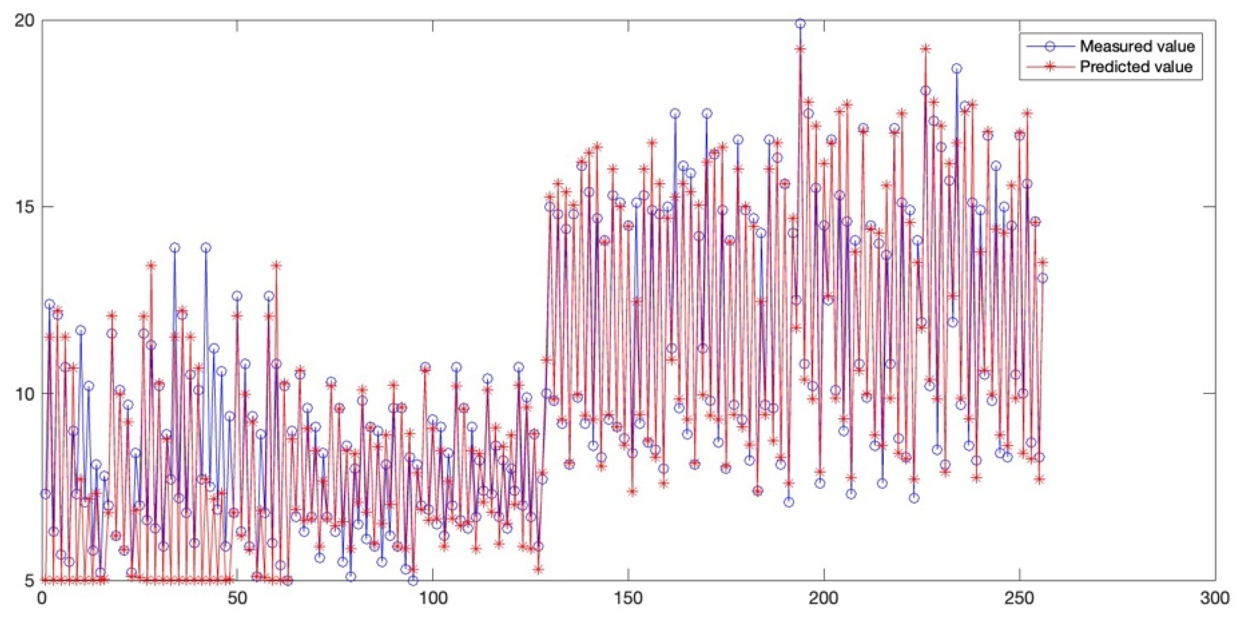
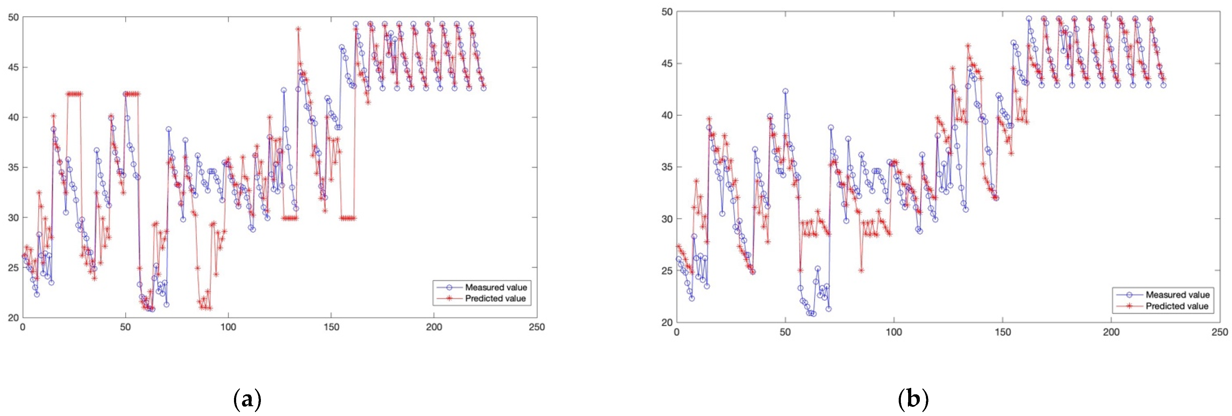
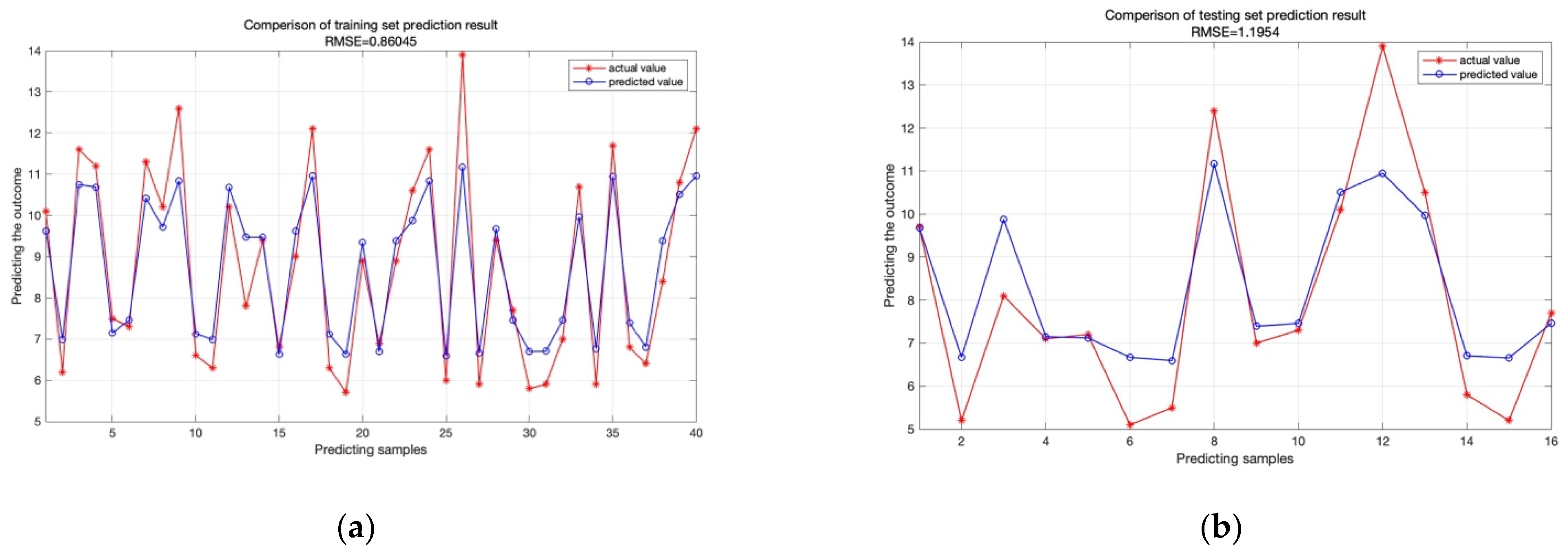
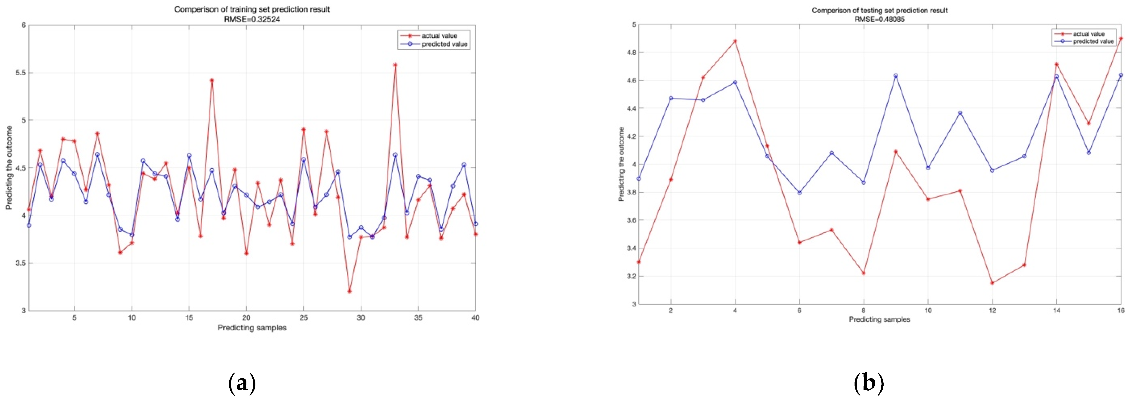
3. Results
4. Discussion
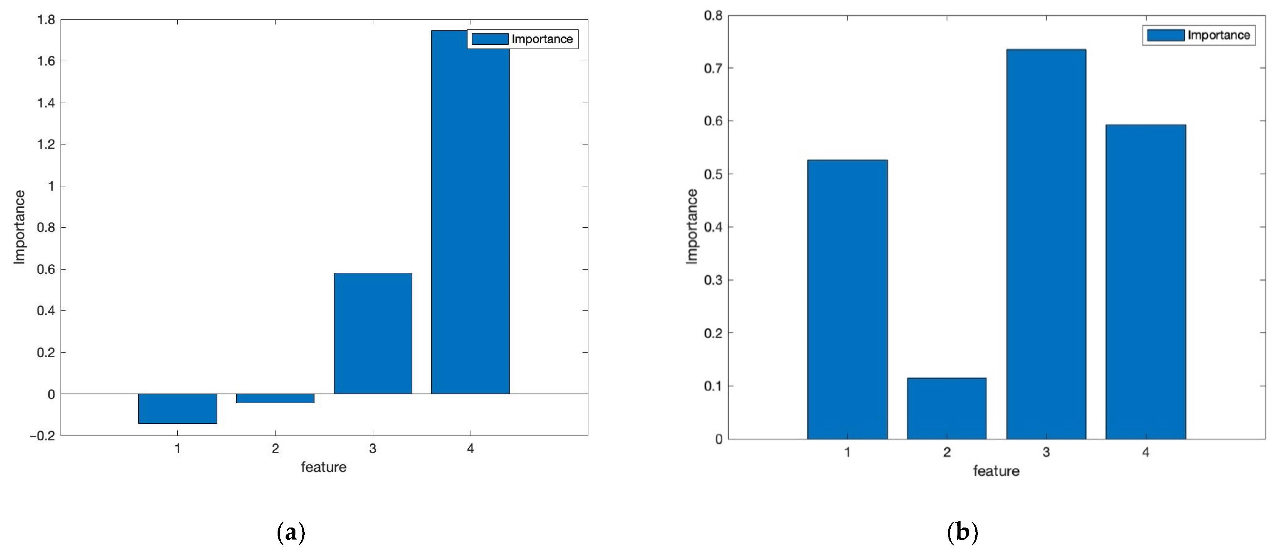
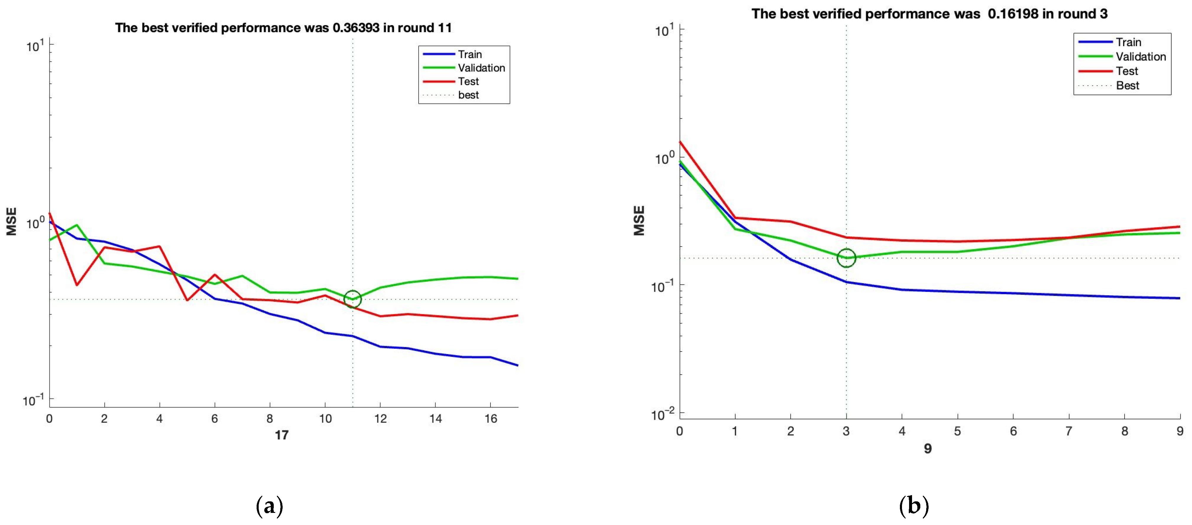
- The four variables of feed rate, wood species, heat treatment time, and heat treatment temperature were varied to varying degrees in this paper. The bond strength values of the two adhesives, PVAc and MUF, were predicted according to varying degrees of changes in different variables. It can be seen from Table 1 that with the increase in temperature, the bonding strength of the PVAc and MUF adhesives gradually decreases, and the value of the PVAc bonding strength decreases significantly between different tree species. Therefore, the CPA-BP model can be used as an efficient method to predict the optimal bond strength of different wood species processed and heat treated under different conditions. Miao SU et al. [21] used an artificial neural network to predict surface-embedded fibers to enhance the bond strength between CFRP and concrete. The established BPNN model has a coefficient of determination R2 of 0.957. Julian D Olden et al. [22] used a Monte Carlo simulation to provide a comparison of the results of different methods. Their paper showed that the average similarity between the actual and predicted values obtained using this method was 0.92; Mário R.F. Coelho et al. [23] proposed a DM model to predict the NSM FRP system, the bond strength of which is more robust and accurate than the guide model, with a minimum RMSE value of 8.6 and an R2 of 0.89. However, the CPA-BP algorithm used in this paper has a better performance in the relationship between the actual value and the predicted value. The coefficient of determination is 0.9771.
- The tree species of the wood is also an important factor affecting the glue strength. Studies have shown that when the wood is glued with the same kind of adhesive, the glue strength also increases proportionally with the density of the tree species. White oak has the greatest bond strength of the four tree species mentioned in this article. On the influence of the direction of wood grain, changing the direction of the fibers on the surface of the plywood, the glued strength will also change accordingly. The bonding strength of the two pieces of wood fiber is the highest when the direction of the wood fibers is parallel, and the bonding strength is the lowest when the direction of the two wood fibers is perpendicular. Ayhan Özçifçi et al. (2008) [24] mentioned in their paper that beech wood has a high density, and its bond strength is better in the tangential direction than in the radial direction. Among all the factors that affect the bonding strength of wood, the relationship between the surface roughness and the bonding strength is relatively complex, and parameters such as wood properties and processing methods may affect the surface roughness, thereby affecting the bonding effect. The bonding strength of the wood surface does not increase linearly with the decrease in the surface roughness. The heat treatment of wood improves its elasticity and mechanical properties, and it is a common process today to maintain the quality of wood by changing its equilibrium moisture content, surface bond strength, surface roughness, etc. In summary, predicting wood properties is relevant to improving wood utilization [25].
5. Conclusions
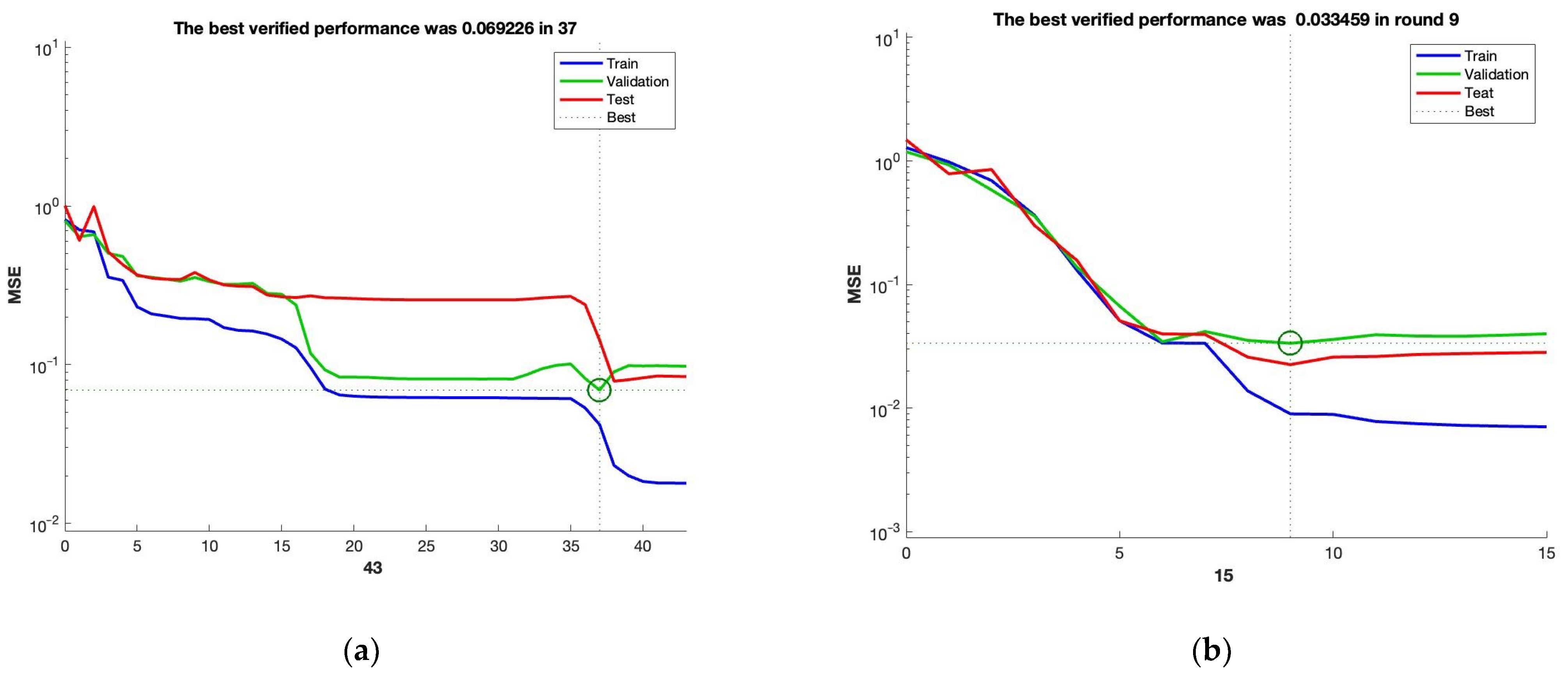
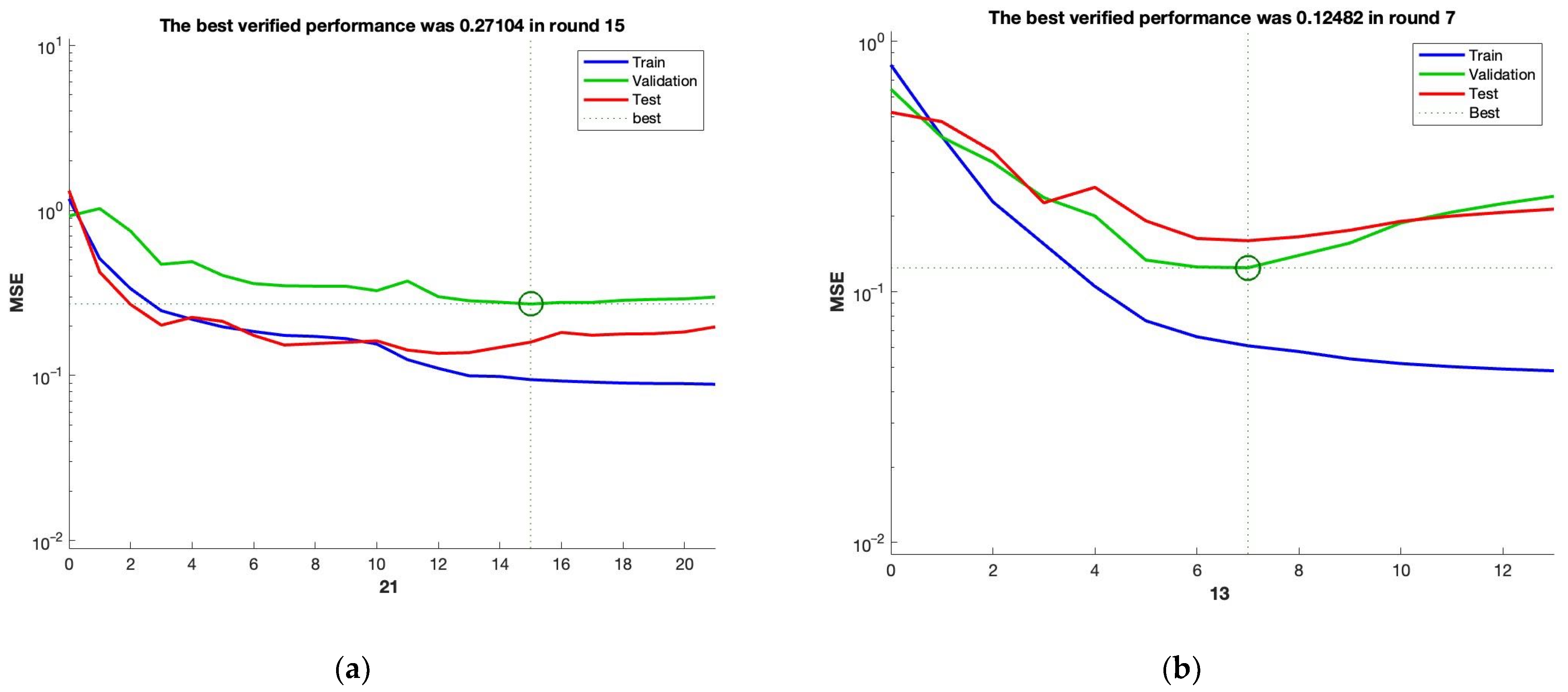
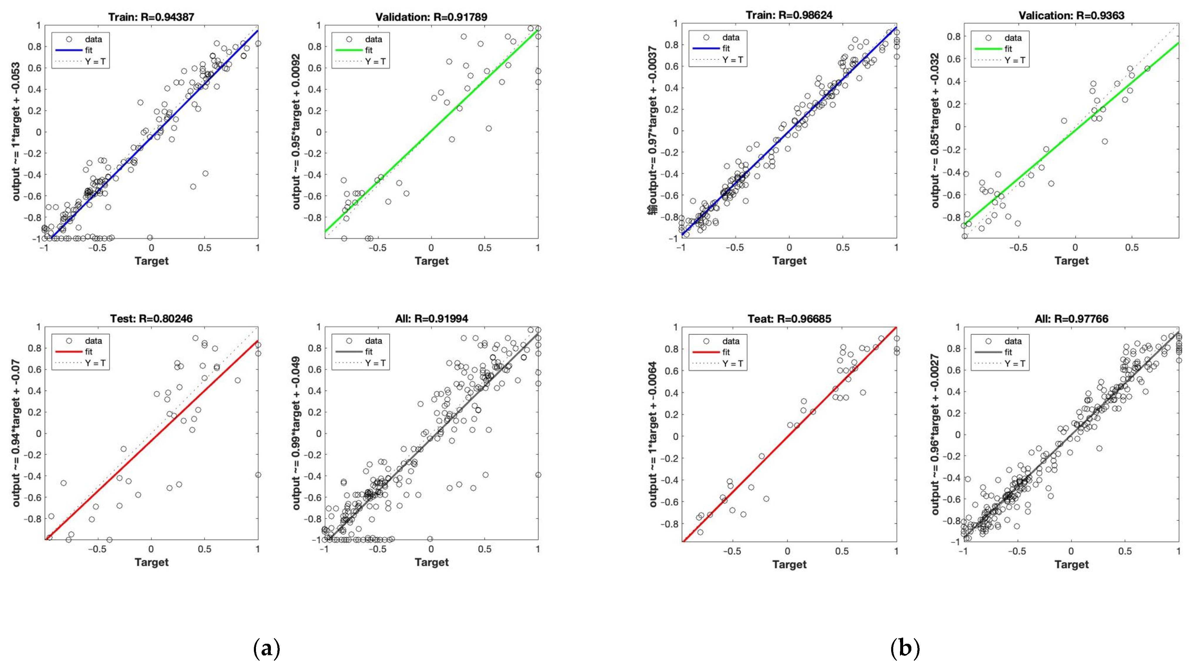
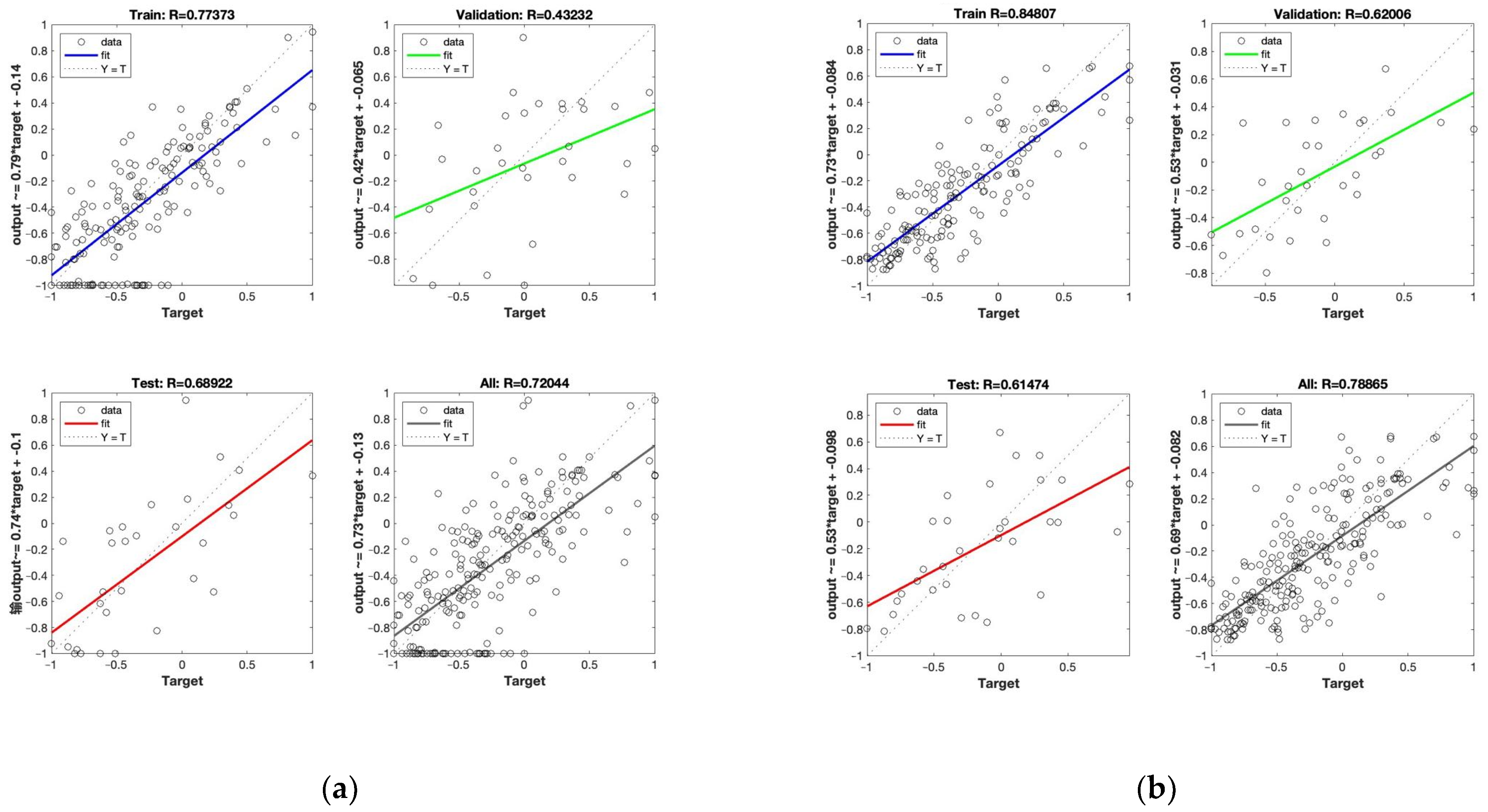
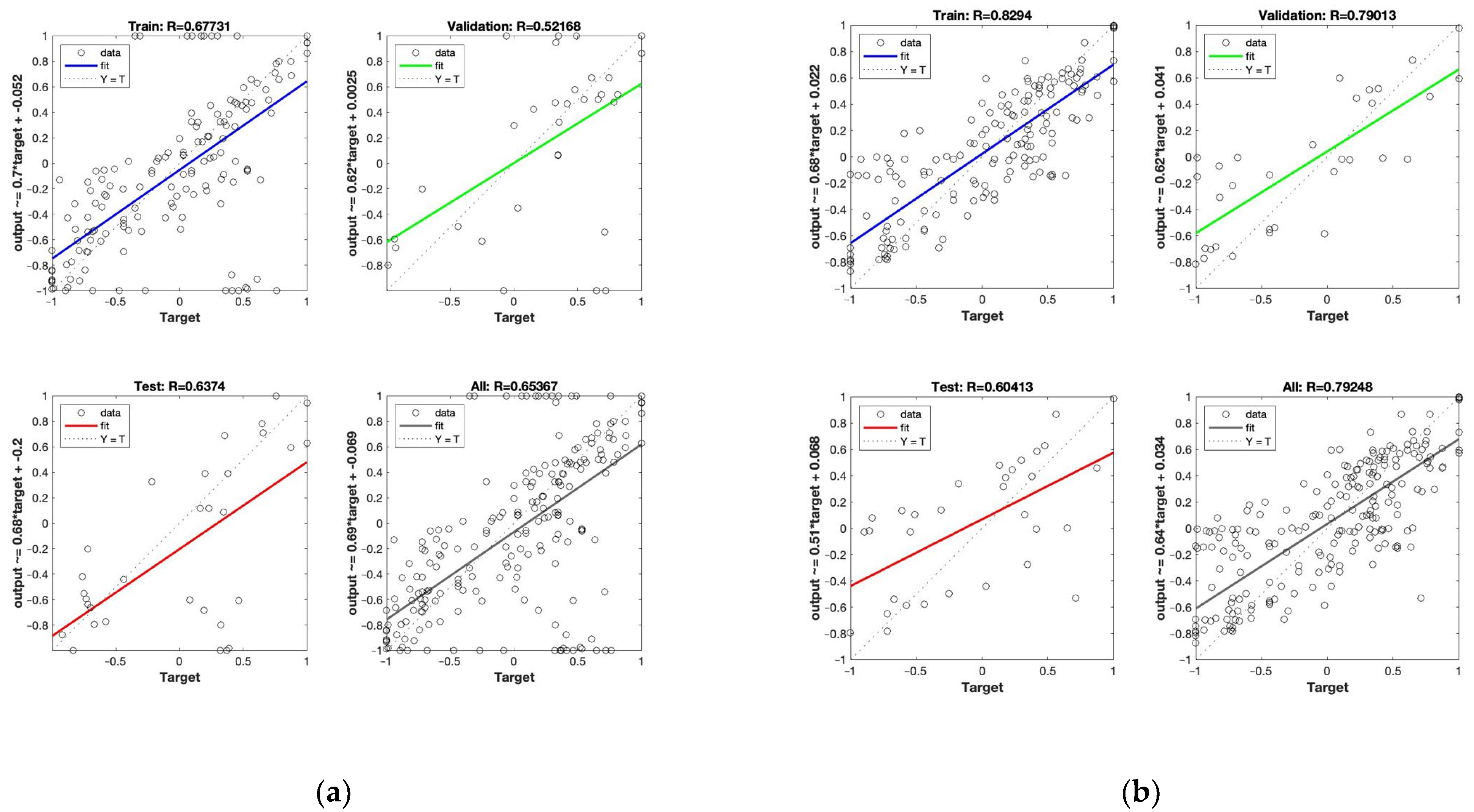
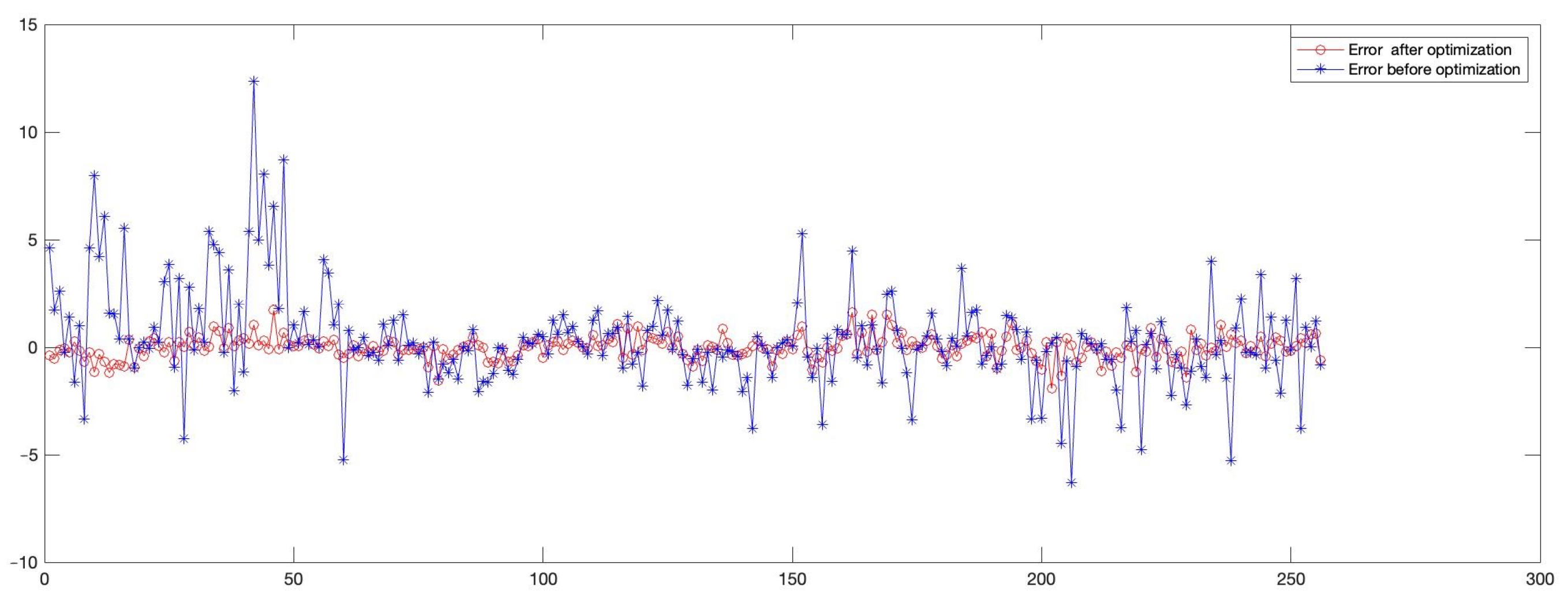
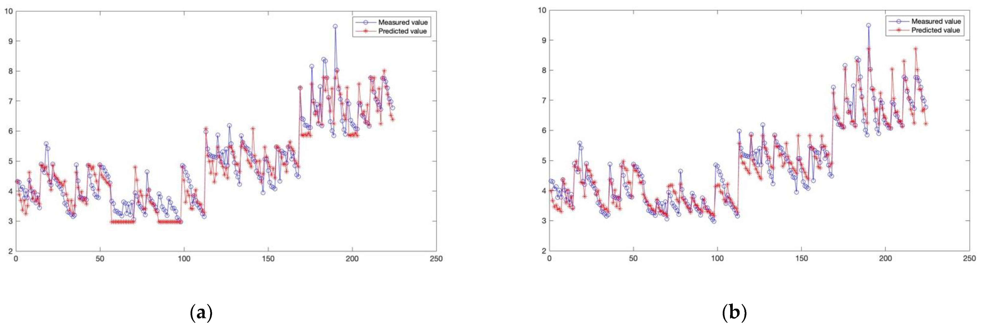
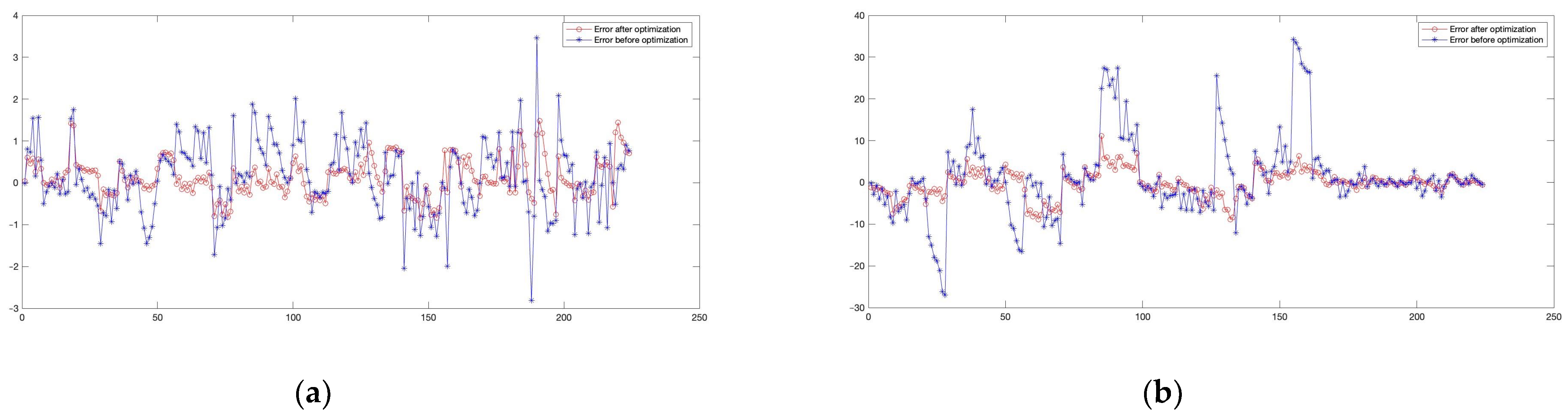
- In this paper, a CPA-BP model was used to predict the bond strength and surface roughness of four kinds of wood with feeding speed, heat treatment time, temperature, and adhesive type as input variables, and they were compared with the actual measured values. The two prediction models used 64 and 56 sets of data, respectively, and were divided into two training and test sets for predicting the bond strength and surface roughness, respectively. The results showed that the optimized bond strength prediction results using the CPA-BP model resulted in a 77.9% decrease in MSE value, a 45.9% decrease in MAE value, a 45.35% decrease in MAPE value, and a 9% increase in R2 value compared to the BP neural network, as well as an 11.9% increase in R2 compared to the random forest algorithm. The surface roughness prediction results showed that the optimized MSE values decreased by up to 54.77%, MAE values decreased by 20.8%, MAPE values decreased by 12.2%, and R2 values increased by 39.4%; compared with the random forest algorithm, R2 increased by up to 55.6%. It can be seen that the algorithm used in this paper has higher accuracy compared to the BP algorithm.
- Combining with the data set used in this paper, there are four types of input, and there is a complex linear relationship between the input and the output. The BP neural network model optimized by CPA has also achieved ideal results in prediction. According to the comparison between the predicted value and the measured value, when the R2 between them is very close to 1, the various error values and MAPE, that is, the average error percentage, are very low. These values illustrate the accuracy and applicability of the CPA-BP algorithm. Compared with the traditional BP neural network model, the algorithm used in this paper is closer to the actual measured value.
- When heat-treating wood, the bond strength values were higher with the PVAc binder under the same tree species and white oak with the same binder. When other conditions are the same, the adhesion performance will gradually decrease with the increase in temperature, among which, the decrease in PVAc is more obvious than that of MUF. When the other conditions are the same, its bond strength is better in the tangential direction than in the radial direction. However, the relationship between surface roughness and wood glue strength is relatively complex.
- In future research, this model can be further optimized. It can be seen that although the CPA-BP model is better than the BP neural network model in predicting the glue strength and surface roughness of plywood, its effect can be better, especially on the surface. In the roughness part, the coefficient of determination R2 of the model is 0.83, and the weights and thresholds in the algorithm can be optimized again so that the prediction results can be closer to the real value and the R2 is higher.
Supplementary Materials
Author Contributions
Funding
Institutional Review Board Statement
Informed Consent Statement
Data Availability Statement
Conflicts of Interest
References
- Cai, J.; Cai, L. Effects of thermal modification on mechanical and swelling properties and color change of lumber killed by mountain pine beetle. Bioresources 2012, 7, 3488–3499. [Google Scholar] [CrossRef]
- Schmidt, M.; Glos, P.; Wegener, G. Gluing of European beech wood for load bearing timber structures. Eur. J. Wood Wood Prod. 2010, 68, 43–57. [Google Scholar] [CrossRef]
- Knorz, M.; Schmidt, M.; Torno, S.; Van De Kuilen, J.-W. Structural bonding of ash (Fraxinus excelsior L.): Resistance to delamination and performance in shearing tests. Holz als Roh-und Werkst. 2014, 72, 297–309. [Google Scholar] [CrossRef]
- Sikora, K.S.; McPolin, D.O.; Harte, A.M. Shear Strength and Durability Testing of Adhesive Bonds in Cross-laminated Timber. J. Adhes. 2015, 92, 758–777. [Google Scholar] [CrossRef] [Green Version]
- Hill, C.; Altgen, M.; Rautkari, L. Thermal modification of wood—A review: Chemical changes and hygroscopicity. J. Mater. Sci. 2021, 56, 6581–6614. [Google Scholar] [CrossRef]
- Kubovský, I.; Kačíková, D.; Kačík, F. Structural Changes of Oak Wood Main Components Caused by Thermal Modification. Polymers 2020, 12, 485. [Google Scholar] [CrossRef] [Green Version]
- Herrera-Builes, J.; Sepúlveda-Villarroel, V.; Osorio, J.; Salvo-Sepúlveda, L.; Ananías, R. Effect of Thermal Modification Treatment on Some Physical and Mechanical Properties of Pinus oocarpa Wood. Forests 2021, 12, 249. [Google Scholar] [CrossRef]
- Wentzel, M.; Fleckenstein, M.; Hofmann, T.; Militz, H. Relation of chemical and mechanical properties of Eucalyptus nitens wood thermally modified in open and closed systems. Wood Mater. Sci. Eng. 2019, 14, 165–173. [Google Scholar] [CrossRef]
- Wang, X.; Chen, X.; Xie, X.; Wu, Y.; Zhao, L.; Li, Y.; Wang, S. Effects of thermal modification on the physical, chemical and micromechanical properties of Masson pine wood (Pinus massoniana Lamb.). Holzforschung 2018, 72, 1063–1070. [Google Scholar] [CrossRef] [Green Version]
- Čabalová, I.; Výbohová, E.; Igaz, R.; Kristak, L.; Kačík, F.; Antov, P.; Papadopoulos, A.N. Effect of oxidizing thermal modification on the chemical properties and thermal conductivity of Norway spruce (Picea abies L.) wood. Wood Mater. Sci. Eng. 2022, 17, 366–375. [Google Scholar] [CrossRef]
- Serrano, E. A numerical study of the shear-strength-predicting capabilities of test specimens for wood–adhesive bonds. Int. J. Adhes. Adhes. 2004, 24, 23–35. [Google Scholar] [CrossRef]
- Esteban, L.G.; Fernández, F.G.; de Palacios, P. Prediction of plywood bonding quality using an artificial neural network. Holzforschung 2011, 65, 209–214. [Google Scholar] [CrossRef]
- Demirkir, C.; Özsahin, Ş.; Aydin, I.; Colakoglu, G. Optimization of some panel manufacturing parameters for the best bonding strength of plywood. Int. J. Adhes. Adhes. 2013, 46, 14–20. [Google Scholar] [CrossRef]
- Ugulino, B.; Hernández, R.E. Assessment of surface properties and solvent-borne coating performance of red oak wood produced by peripheral planing. Eur. J. Wood Wood Prod. 2017, 75, 581–593. [Google Scholar] [CrossRef]
- Hazir, E.; Ozcan, T.; Koç, K.H. Prediction of Adhesion Strength Using Extreme Learning Machine and Support Vector Regression Optimized with Genetic Algorithm. Arab. J. Sci. Eng. 2020, 45, 6985–7004. [Google Scholar] [CrossRef]
- Ozcan, S.; Ozcifci, A.; Hiziroglu, S.; Toker, H. Effects of heat treatment and surface roughness on bonding strength. Constr. Build. Mater. 2012, 33, 7–13. [Google Scholar] [CrossRef]
- Ong, K.M.; Ong, P.; Sia, C.K. A carnivorous plant algorithm for solving global optimization problems. Appl. Soft Comput. 2020, 98, 106833. [Google Scholar] [CrossRef]
- Tiryaki, S.; Özşahin, Ş.; Yıldırım, I. Comparison of artificial neural network and multiple linear regression models to predict optimum bonding strength of heat treated woods. Int. J. Adhes. Adhes. 2014, 55, 29–36. [Google Scholar] [CrossRef]
- Kohonen, T.; Mäkisara, K.; Simula, O.; Kangas, J. (Eds.) Artificial Neural Networks; Elsevier: Amsterdam, The Netherlands, 1991. [Google Scholar] [CrossRef]
- Cutler, D.R.; Edwards, T.C., Jr.; Beard, K.H.; Cutler, A.; Hess, K.T.; Gibson, J.; Lawler, J.J. Random forests for classification in ecology. Ecology 2007, 88, 2783–2792. [Google Scholar] [CrossRef]
- Su, M.; Peng, H.; Li, S.-F. Application of an interpretable artificial neural network to predict the interface strength of a near-surface mounted fiber-reinforced polymer to concrete joint. J. Zhejiang Univ. A 2021, 22, 427–440. [Google Scholar] [CrossRef]
- Olden, J.D.; Joy, M.K.; Death, R.G. An accurate comparison of methods for quantifying variable importance in artificial neural networks using simulated data. Ecol. Model. 2004, 178, 389–397. [Google Scholar] [CrossRef]
- Coelho, M.R.; Sena-Cruz, J.M.; Neves, L.A.; Pereira, M.; Cortez, P.; Miranda, T. Using data mining algorithms to predict the bond strength of NSM FRP systems in concrete. Constr. Build. Mater. 2016, 126, 484–495. [Google Scholar] [CrossRef]
- Özçifçi, A.; Yapici, F. Effects of machining method and grain orientation on the bonding strength of some wood species. J. Mater. Process. Technol. 2008, 202, 353–358. [Google Scholar] [CrossRef]
- Chen, Y.; Wang, W.; Li, N. Prediction of the equilibrium moisture content and specific gravity of thermally modified wood via an Aquila optimization algorithm back-propagation neural network model. BioResources 2022, 17, 4816–4836. [Google Scholar] [CrossRef]


| Group Statistics | |||||
|---|---|---|---|---|---|
| Adhesives | N | average value | Standard deviation | Standard error mean | |
| ScotchPine | 0.00 | 32 | 6.3531 | 0.79189 | 0.13999 |
| 1.00 | 32 | 10.6188 | 1.56750 | 0.27710 | |
| Independent Sample Test | |||||||||
|---|---|---|---|---|---|---|---|---|---|
| Levin’s test of variance equality | Mean equality t-test | ||||||||
| ScotchPine | F | Significance | t | degree of freedom | Significance (two-tailed) | Mean Difference | Standard error difference | Difference 95% confidence interval | |
| Lower limit | Upper limit | ||||||||
| Assuming equal variance | 10.641 | 0.002 | −13.740 | 62 | 0.000 | −4.26563 | 0.31045 | −4.88621 | −3.64504 |
| Does not assume equal variance | −13.740 | 45.856 | 0.000 | −4.26563 | 0.31045 | −4.89058 | −3.64067 | ||
| Scotch Pine | Sum of Squares | Degree of Freedom | Mean Square | F | Significance |
|---|---|---|---|---|---|
| SSA | 62.747 | 3 | 20.916 | 3.873 | 0.013 |
| SSE | 323.991 | 60 | 5.400 | ||
| SST | 386.737 | 63 |
| (I) Temp | (J) Temp | Mean Difference (I–J) | Standard Error | Significance | 95% Confidence Interval | |
|---|---|---|---|---|---|---|
| Lower Limit | Upper Limit | |||||
| 0.00 | 1.00 | 1.00625 | 0.82157 | 0.225 | −0.6371 | 2.6496 |
| 2.00 | 1.86250 * | 0.82157 | 0.027 | 0.2191 | 3.5059 | |
| 3.00 | 2.66250 * | 0.82157 | 0.002 | 1.0191 | 4.3059 | |
| 1.00 | 0.00 | −1.00625 | 0.82157 | 0.225 | −2.6496 | 0.6371 |
| 2.00 | 0.85625 | 0.82157 | 0.301 | −0.7871 | 2.4996 | |
| 3.00 | 1.65625 * | 0.82157 | 0.048 | 0.0129 | 3.2996 | |
| 2.00 | 0.00 | −1.86250 * | 0.82157 | 0.027 | −3.5059 | −0.2191 |
| 1.00 | −0.85625 | 0.82157 | 0.301 | −2.4996 | 0.7871 | |
| 3.00 | 0.80000 | 0.82157 | 0.334 | −0.8434 | 2.4434 | |
| 3.00 | 0.00 | −2.66250 * | 0.82157 | 0.002 | −4.3059 | −1.0191 |
| 1.00 | −1.65625 * | 0.82157 | 0.048 | −3.2996 | −0.0129 | |
| 2.00 | −0.80000 | 0.82157 | 0.334 | −2.4434 | 0.8434 | |
| Grain Orientation | Feeding Speed | Duration | Temperature | Adhesives | Measured | Predicted | Measured | Predicted | Measured | Predicted | Measured | Predicted |
|---|---|---|---|---|---|---|---|---|---|---|---|---|
| Scotch Pine | Uludag Fir | Oriental Beech | White Oak | |||||||||
| Radial | 8 m/min | 2 | control | MUF | 7.3000 | 7.6794 | 6.7000 | 6.9424 | 10.0000 | 10.5935 | 12.5000 | 11.9949 |
| PVAc | 12.4000 | 12.9384 | 10.5000 | 10.4530 | 15.0000 | 15.8804 | 19.9000 | 18.7821 | ||||
| 120 °C | MUF | 6.3000 | 6.4347 | 6.3000 | 6.5158 | 9.8000 | 9.9229 | 10.8000 | 10.9303 | |||
| PVAc | 12.1000 | 12.1663 | 9.6000 | 9.7772 | 14.8000 | 15.4382 | 17.5000 | 17.5013 | ||||
| 150 °C | MUF | 5.7000 | 5.9203 | 6.7000 | 6.4052 | 9.2000 | 9.0955 | 10.2000 | 9.8968 | |||
| PVAc | 10.7000 | 10.4410 | 9.1000 | 8.8727 | 14.4000 | 14.3814 | 15.5000 | 15.7770 | ||||
| 180 °C | MUF | 5.5000 | 5.6752 | 5.6000 | 5.9294 | 8.1000 | 8.2383 | 7.6000 | 8.2307 | |||
| PVAc | 9.0000 | 9.6808 | 8.4000 | 8.5099 | 14.8000 | 13.9525 | 14.5000 | 15.5375 | ||||
| 4 | control | MUF | 7.3000 | 7.5344 | 6.7000 | 6.8204 | 9.9000 | 9.6859 | 12.5000 | 12.2787 | ||
| PVAc | 11.7000 | 12.8628 | 10.3000 | 10.4035 | 16.1000 | 16.4593 | 16.8000 | 18.7292 | ||||
| 120 °C | MUF | 7.1000 | 7.4255 | 6.3000 | 6.3918 | 9.2000 | 9.5855 | 10.1000 | 9.8694 | |||
| PVAc | 10.2000 | 10.8839 | 9.6000 | 9.6280 | 15.4000 | 15.7163 | 15.3000 | 16.6434 | ||||
| 150 °C | MUF | 5.8000 | 6.9837 | 5.5000 | 6.4414 | 8.6000 | 8.8279 | 9.0000 | 8.5835 | |||
| PVAc | 8.1000 | 8.8735 | 8.6000 | 8.5327 | 14.7000 | 14.6435 | 14.6000 | 14.5109 | ||||
| 180 °C | MUF | 5.2000 | 6.0050 | 5.1000 | 6.6618 | 8.3000 | 7.9627 | 7.3000 | 8.0013 | |||
| PVAc | 7.8000 | 8.7073 | 8.0000 | 8.0996 | 14.1000 | 14.1328 | 14.1000 | 14.6037 | ||||
| 16 m/min | 2 | control | MUF | 7.0000 | 6.6605 | 6.5000 | 7.0236 | 9.3000 | 9.3826 | 10.8000 | 10.7860 | |
| PVAc | 11.6000 | 12.5449 | 9.8000 | 10.1550 | 15.3000 | 16.1866 | 17.1000 | 16.8517 | ||||
| 120 °C | MUF | 6.2000 | 6.2485 | 6.1000 | 6.2210 | 9.1000 | 9.2409 | 9.9000 | 9.9950 | |||
| PVAc | 10.1000 | 10.5053 | 9.1000 | 9.0906 | 15.1000 | 15.4207 | 14.5000 | 15.5957 | ||||
| 150 °C | MUF | 5.8000 | 5.5346 | 5.9000 | 5.8056 | 8.8000 | 8.5312 | 8.6000 | 8.8172 | |||
| PVAc | 9.7000 | 9.2768 | 9.0000 | 8.5314 | 14.5000 | 14.6034 | 14.0000 | 14.8537 | ||||
| 180 °C | MUF | 5.2000 | 5.1466 | 5.5000 | 5.4186 | 8.4000 | 7.8365 | 7.6000 | 7.8345 | |||
| PVAc | 8.4000 | 8.6401 | 8.1000 | 8.1266 | 15.1000 | 14.1342 | 13.7000 | 14.2061 | ||||
| 4 | control | MUF | 7.0000 | 6.7588 | 6.2000 | 6.9059 | 9.2000 | 9.3938 | 10.8000 | 10.7105 | ||
| PVAc | 11.6000 | 12.2452 | 9.6000 | 10.2657 | 15.3000 | 16.3239 | 17.1000 | 17.0773 | ||||
| 120 °C | MUF | 6.6000 | 6.3451 | 5.9000 | 6.6460 | 8.7000 | 9.1959 | 8.8000 | 9.9380 | |||
| PVAc | 11.3000 | 11.2903 | 9.6000 | 9.7277 | 14.9000 | 15.5982 | 15.1000 | 15.1886 | ||||
| 150 °C | MUF | 6.4000 | 5.6998 | 5.3000 | 5.9860 | 8.5000 | 8.5284 | 8.3000 | 8.5077 | |||
| PVAc | 10.2000 | 10.0936 | 8.3000 | 8.9364 | 14.8000 | 14.9623 | 14.9000 | 14.0068 | ||||
| 180 °C | MUF | 5.9000 | 5.4324 | 5.0000 | 5.3976 | 8.0000 | 8.0672 | 7.2000 | 7.6578 | |||
| PVAc | 8.9000 | 9.0611 | 8.1000 | 8.0123 | 15.0000 | 14.4797 | 14.1000 | 13.7108 | ||||
| Tangential | 8 m/min | 2 | control | MUF | 7.7000 | 7.6794 | 7.0000 | 6.9424 | 11.2000 | 10.5935 | 11.9000 | 11.9949 |
| PVAc | 13.9000 | 12.9384 | 10.7000 | 10.4530 | 17.5000 | 15.8804 | 18.1000 | 18.7821 | ||||
| 120 °C | MUF | 7.2000 | 6.4347 | 6.9000 | 6.5158 | 9.6000 | 9.9229 | 10.2000 | 10.9303 | |||
| PVAc | 12.1000 | 12.1663 | 9.3000 | 9.7772 | 16.1000 | 15.4382 | 17.3000 | 17.5013 | ||||
| 150 °C | MUF | 6.8000 | 5.9203 | 6.5000 | 6.4052 | 8.9000 | 9.0955 | 8.5000 | 9.8968 | |||
| PVAc | 10.5000 | 10.4410 | 9.1000 | 8.8727 | 15.9000 | 14.3814 | 16.6000 | 15.7770 | ||||
| 180 °C | MUF | 6.0000 | 5.6752 | 6.2000 | 5.9294 | 8.1000 | 8.2383 | 8.1000 | 8.2307 | |||
| PVAc | 10.1000 | 9.6808 | 8.4000 | 8.5099 | 14.2000 | 13.9525 | 15.7000 | 15.5375 | ||||
| 4 | control | MUF | 7.7000 | 7.5344 | 7.0000 | 6.8204 | 11.2000 | 9.6859 | 11.9000 | 12.2787 | ||
| PVAc | 13.9000 | 12.8628 | 10.7000 | 10.4035 | 17.5000 | 16.4593 | 18.7000 | 18.7292 | ||||
| 120 °C | MUF | 7.5000 | 7.4255 | 6.6000 | 6.3918 | 9.8000 | 9.5855 | 9.7000 | 9.8694 | |||
| PVAc | 11.2000 | 10.8839 | 9.6000 | 9.6280 | 16.4000 | 15.7163 | 17.7000 | 16.6434 | ||||
| 150 °C | MUF | 6.9000 | 6.9837 | 6.4000 | 6.4414 | 8.7000 | 8.8279 | 8.6000 | 8.5835 | |||
| PVAc | 10.6000 | 8.8735 | 9.1000 | 8.5327 | 14.9000 | 14.6435 | 15.1000 | 14.5109 | ||||
| 180 °C | MUF | 5.9000 | 6.0050 | 6.7000 | 6.6618 | 8.0000 | 7.9627 | 8.2000 | 8.0013 | |||
| PVAc | 9.4000 | 8.7073 | 8.2000 | 8.0996 | 14.1000 | 14.1328 | 14.9000 | 14.6037 | ||||
| 16 m/min | 2 | control | MUF | 6.8000 | 6.6605 | 7.4000 | 7.0236 | 9.7000 | 9.3826 | 10.5000 | 10.7860 | |
| PVAc | 12.6000 | 12.5449 | 10.4000 | 10.1550 | 16.8000 | 16.1866 | 16.9000 | 16.8517 | ||||
| 120 °C | MUF | 6.3000 | 6.2485 | 7.3000 | 6.2210 | 9.3000 | 9.2409 | 9.8000 | 9.9950 | |||
| PVAc | 10.8000 | 10.5053 | 8.6000 | 9.0906 | 14.9000 | 15.4207 | 16.1000 | 15.5957 | ||||
| 150 °C | MUF | 5.9000 | 5.5346 | 6.7000 | 5.8056 | 8.2000 | 8.5312 | 8.4000 | 8.8172 | |||
| PVAc | 9.4000 | 9.2768 | 8.2000 | 8.5314 | 14.7000 | 14.6034 | 15.0000 | 14.8537 | ||||
| 180 °C | MUF | 5.1000 | 5.1466 | 6.4000 | 5.4186 | 7.4000 | 7.8365 | 8.3000 | 7.8345 | |||
| PVAc | 8.9000 | 8.6401 | 8.0000 | 8.1266 | 14.3000 | 14.1342 | 14.5000 | 14.2061 | ||||
| 4 | control | MUF | 6.8000 | 6.7588 | 7.4000 | 6.9059 | 9.7000 | 9.3938 | 10.5000 | 10.7105 | ||
| PVAc | 12.6000 | 12.2452 | 10.7000 | 10.2657 | 16.8000 | 16.3239 | 16.9000 | 17.0773 | ||||
| 120 °C | MUF | 6.0000 | 6.3451 | 7.0000 | 6.6460 | 9.6000 | 9.1959 | 10.0000 | 9.9380 | |||
| PVAc | 10.8000 | 11.2903 | 9.9000 | 9.7277 | 16.3000 | 15.5982 | 15.6000 | 15.1886 | ||||
| 150 °C | MUF | 5.4000 | 5.6998 | 6.7000 | 5.9860 | 8.1000 | 8.5284 | 8.7000 | 8.5077 | |||
| PVAc | 10.2000 | 10.0936 | 8.9000 | 8.9364 | 15.6000 | 14.9623 | 14.6000 | 14.0068 | ||||
| 180 °C | MUF | 5.0000 | 5.4324 | 5.9000 | 5.3976 | 7.1000 | 8.0672 | 8.3000 | 7.6578 | |||
| PVAc | 9.0000 | 9.0611 | 7.7000 | 8.0123 | 14.3000 | 14.4797 | 13.1000 | 13.7108 | ||||
| Grain Orientation | Feeding Speed | Time | Temp. | Process | Scotch Pine | Uludag Fir | Oriental Beech | White Oak | ||||
|---|---|---|---|---|---|---|---|---|---|---|---|---|
| Ra | Predicted Value | Ra | Predicted Value | Ra | Predicted Value | Ra | Predicted Value | |||||
| Radial | 8 m/min | 2 h | Contr | 4.320 | 3.993 | 3.670 | 3.765 | 5.980 | 5.563 | 7.440 | 7.239 | |
| 120 °C | b-ht | 4.290 | 3.661 | 3.580 | 3.648 | 5.400 | 5.123 | 6.420 | 6.735 | |||
| a-ht | 4.060 | 3.454 | 3.340 | 3.508 | 5.220 | 4.919 | 6.390 | 6.489 | ||||
| 150 °C | b-ht | 4.130 | 3.515 | 3.320 | 3.497 | 5.170 | 4.909 | 6.200 | 6.413 | |||
| a-ht | 3.770 | 3.370 | 3.270 | 3.391 | 5.160 | 4.740 | 6.190 | 6.227 | ||||
| 180 °C | b-ht | 4.020 | 3.398 | 3.250 | 3.354 | 5.140 | 4.673 | 6.120 | 6.186 | |||
| a-ht | 3.780 | 3.307 | 3.170 | 3.292 | 5.120 | 4.573 | 6.120 | 6.079 | ||||
| 6 h | Contr | 4.370 | 4.363 | 3.640 | 3.707 | 5.870 | 5.821 | 8.160 | 8.028 | |||
| 120 °C | b-ht | 4.010 | 4.221 | 3.590 | 3.434 | 5.240 | 5.017 | 7.010 | 7.063 | |||
| a-ht | 3.700 | 3.594 | 3.260 | 3.298 | 4.970 | 4.864 | 6.610 | 6.595 | ||||
| 150 °C | b-ht | 3.970 | 4.009 | 3.570 | 3.329 | 5.310 | 4.716 | 6.890 | 6.614 | |||
| a-ht | 3.610 | 3.477 | 3.210 | 3.220 | 4.860 | 4.594 | 6.250 | 6.289 | ||||
| 180 °C | b-ht | 3.870 | 3.798 | 3.630 | 3.239 | 5.400 | 4.458 | 7.480 | 6.307 | |||
| a-ht | 3.440 | 3.397 | 3.060 | 3.167 | 4.860 | 4.393 | 6.170 | 6.130 | ||||
| 16 m/min | 2 h | Contr | 4.900 | 4.800 | 3.940 | 4.134 | 6.190 | 5.827 | 8.390 | 8.300 | ||
| 120 °C | b-ht | 4.715 | 4.969 | 3.830 | 4.178 | 5.580 | 5.424 | 8.340 | 7.674 | |||
| a-ht | 4.620 | 4.733 | 3.580 | 4.181 | 5.270 | 5.385 | 7.780 | 7.364 | ||||
| 150 °C | b-ht | 5.580 | 4.685 | 3.490 | 3.972 | 4.950 | 5.130 | 7.120 | 7.076 | |||
| a-ht | 5.420 | 4.275 | 3.430 | 3.915 | 4.620 | 5.083 | 6.320 | 6.697 | ||||
| 180 °C | b-ht | 4.310 | 4.262 | 3.340 | 3.704 | 4.470 | 4.793 | 6.010 | 6.532 | |||
| a-ht | 4.200 | 3.800 | 3.210 | 3.614 | 4.230 | 4.752 | 5.850 | 6.251 | ||||
| 6 h | Contr | 4.900 | 4.838 | 4.650 | 4.213 | 5.850 | 5.808 | 9.490 | 8.709 | |||
| 120 °C | b-ht | 4.440 | 4.666 | 4.040 | 3.774 | 5.630 | 5.460 | 8.030 | 8.026 | |||
| a-ht | 4.380 | 4.656 | 3.750 | 3.688 | 5.510 | 5.471 | 7.400 | 7.368 | ||||
| 150 °C | b-ht | 4.220 | 4.509 | 3.660 | 3.586 | 5.440 | 5.155 | 7.060 | 7.352 | |||
| a-ht | 4.160 | 4.255 | 3.550 | 3.456 | 5.400 | 5.208 | 6.340 | 6.637 | ||||
| 180 °C | b-ht | 4.070 | 4.281 | 3.470 | 3.402 | 5.250 | 4.810 | 6.050 | 6.714 | |||
| a-ht | 3.900 | 3.873 | 3.350 | 3.279 | 5.180 | 4.909 | 5.900 | 6.221 | ||||
| Tangential | 8 m/min | 2 h | Contr | 3.600 | 3.993 | 3.910 | 3.765 | 5.060 | 5.563 | 7.000 | 7.239 | |
| 120 °C | b-ht | 3.530 | 3.661 | 3.810 | 3.648 | 5.000 | 5.123 | 6.910 | 6.735 | |||
| a-ht | 3.300 | 3.454 | 3.480 | 3.508 | 4.670 | 4.919 | 6.360 | 6.489 | ||||
| 150 °C | b-ht | 3.280 | 3.515 | 3.380 | 3.497 | 4.590 | 4.909 | 6.230 | 6.413 | |||
| a-ht | 3.220 | 3.370 | 3.320 | 3.391 | 4.450 | 4.740 | 6.170 | 6.227 | ||||
| 180 °C | b-ht | 3.150 | 3.398 | 3.180 | 3.354 | 4.420 | 4.673 | 6.080 | 6.186 | |||
| a-ht | 3.200 | 3.307 | 3.760 | 3.292 | 3.950 | 4.573 | 6.070 | 6.079 | ||||
| 6 h | Contr | 4.880 | 4.363 | 3.620 | 3.707 | 5.060 | 5.821 | 6.940 | 8.028 | |||
| 120 °C | b-ht | 4.340 | 4.221 | 3.430 | 3.434 | 5.060 | 5.017 | 6.880 | 7.063 | |||
| a-ht | 3.800 | 3.594 | 3.430 | 3.298 | 4.680 | 4.864 | 6.530 | 6.595 | ||||
| 150 °C | b-ht | 3.770 | 4.009 | 3.330 | 3.329 | 4.290 | 4.716 | 6.470 | 6.614 | |||
| a-ht | 3.760 | 3.477 | 3.120 | 3.220 | 4.160 | 4.594 | 6.300 | 6.289 | ||||
| 180 °C | b-ht | 3.750 | 3.798 | 3.030 | 3.239 | 4.120 | 4.458 | 6.270 | 6.307 | |||
| a-ht | 3.710 | 3.397 | 2.970 | 3.167 | 4.070 | 4.393 | 6.160 | 6.130 | ||||
| 16 m/min | 2 h | Contr | 4.860 | 4.800 | 4.850 | 4.134 | 5.480 | 5.827 | 7.780 | 8.300 | ||
| 120 °C | b-ht | 4.500 | 4.969 | 4.810 | 4.178 | 5.400 | 5.424 | 7.720 | 7.674 | |||
| a-ht | 4.190 | 4.733 | 4.630 | 4.181 | 4.330 | 5.385 | 7.300 | 7.364 | ||||
| 150 °C | b-ht | 4.090 | 4.685 | 4.520 | 3.972 | 5.330 | 5.130 | 7.060 | 7.076 | |||
| a-ht | 3.890 | 4.275 | 4.340 | 3.915 | 5.280 | 5.083 | 6.970 | 6.697 | ||||
| 180 °C | b-ht | 3.810 | 4.262 | 4.140 | 3.704 | 5.250 | 4.793 | 6.880 | 6.532 | |||
| a-ht | 3.780 | 3.800 | 3.570 | 3.614 | 4.940 | 4.752 | 6.720 | 6.251 | ||||
| 6 h | Contr | 4.880 | 4.838 | 3.850 | 4.213 | 5.480 | 5.808 | 7.760 | 8.709 | |||
| 120 °C | b-ht | 4.800 | 4.666 | 3.690 | 3.774 | 5.400 | 5.460 | 7.750 | 8.026 | |||
| a-ht | 4.780 | 4.656 | 3.540 | 3.688 | 5.070 | 5.471 | 7.650 | 7.368 | ||||
| 150 °C | b-ht | 4.680 | 4.509 | 3.450 | 3.586 | 5.270 | 5.155 | 7.440 | 7.352 | |||
| a-ht | 4.550 | 4.255 | 3.370 | 3.456 | 4.840 | 5.208 | 7.080 | 6.637 | ||||
| 180 °C | b-ht | 4.480 | 4.281 | 3.240 | 3.402 | 4.540 | 4.810 | 6.980 | 6.714 | |||
| a-ht | 4.270 | 3.873 | 3.150 | 3.279 | 4.480 | 4.909 | 6.770 | 6.221 | ||||
| Grain Orientation | Feeding Speed | Time | Temp. | Process | Scotch Pine | Uludag Fir | Oriental Beech | White Oak | ||||
|---|---|---|---|---|---|---|---|---|---|---|---|---|
| Rmax | Predicted Value | Rmax | Predicted Value | Rmax | Predicted Value | Rmax | Predicted Value | |||||
| Radial | 8 m/min | 2 h | Contr | 26.100 | 26.073 | 23.300 | 23.573 | 36.200 | 36.258 | 49.300 | 49.232 | |
| 120 °C | b-ht | 25.600 | 26.919 | 22.100 | 27.559 | 34.000 | 36.147 | 48.900 | 48.245 | |||
| a-ht | 25.000 | 26.135 | 21.900 | 29.062 | 33.000 | 33.944 | 46.200 | 46.136 | ||||
| 150 °C | b-ht | 24.800 | 25.778 | 21.500 | 29.086 | 32.200 | 33.596 | 45.400 | 46.063 | |||
| a-ht | 23.800 | 24.925 | 20.900 | 29.747 | 31.000 | 31.947 | 44.700 | 44.069 | ||||
| 180 °C | b-ht | 23.000 | 24.639 | 20.900 | 30.666 | 30.500 | 31.809 | 43.800 | 43.926 | |||
| a-ht | 22.300 | 24.158 | 20.800 | 29.069 | 29.900 | 30.994 | 42.900 | 43.289 | ||||
| 6 h | Contr | 28.300 | 32.319 | 23.900 | 29.524 | 38.000 | 39.676 | 49.300 | 49.010 | |||
| 120 °C | b-ht | 26.200 | 32.844 | 25.200 | 31.187 | 34.300 | 40.759 | 47.900 | 48.653 | |||
| a-ht | 24.400 | 30.033 | 22.600 | 29.763 | 32.800 | 37.318 | 46.200 | 46.378 | ||||
| 150 °C | b-ht | 26.400 | 30.039 | 23.300 | 28.741 | 35.300 | 38.167 | 48.400 | 47.592 | |||
| a-ht | 24.100 | 28.912 | 22.400 | 29.346 | 32.600 | 37.111 | 44.700 | 44.168 | ||||
| 180 °C | b-ht | 26.200 | 28.570 | 23.500 | 27.241 | 36.600 | 37.725 | 47.800 | 45.221 | |||
| a-ht | 23.500 | 28.009 | 21.300 | 29.098 | 33.200 | 36.970 | 42.900 | 43.169 | ||||
| 16 m/min | 2 h | Contr | 38.800 | 39.121 | 38.800 | 35.434 | 42.700 | 46.643 | 49.300 | 49.214 | ||
| 120 °C | b-ht | 37.800 | 37.697 | 36.500 | 36.140 | 38.800 | 40.927 | 48.300 | 48.000 | |||
| a-ht | 36.800 | 36.526 | 35.900 | 34.994 | 37.000 | 37.363 | 46.200 | 45.754 | ||||
| 150 °C | b-ht | 35.500 | 35.719 | 34.500 | 34.247 | 35.000 | 40.381 | 45.400 | 45.872 | |||
| a-ht | 34.500 | 35.401 | 33.300 | 33.557 | 33.000 | 39.230 | 44.700 | 43.787 | ||||
| 180 °C | b-ht | 33.900 | 33.865 | 33.200 | 32.343 | 31.500 | 41.866 | 43.800 | 43.735 | |||
| a-ht | 30.500 | 33.775 | 31.400 | 31.634 | 30.900 | 41.084 | 42.900 | 43.111 | ||||
| 6 h | Contr | 35.800 | 39.207 | 29.800 | 30.771 | 42.800 | 46.784 | 49.300 | 48.601 | |||
| 120 °C | b-ht | 34.800 | 38.369 | 37.700 | 34.712 | 44.500 | 46.955 | 48.500 | 47.863 | |||
| a-ht | 33.300 | 36.376 | 34.900 | 33.881 | 43.800 | 45.093 | 46.200 | 46.629 | ||||
| 150 °C | b-ht | 32.900 | 36.771 | 34.200 | 33.121 | 43.500 | 45.472 | 45.400 | 46.336 | |||
| a-ht | 31.700 | 34.178 | 33.000 | 32.603 | 41.100 | 43.566 | 44.700 | 44.377 | ||||
| 180 °C | b-ht | 29.200 | 34.722 | 32.700 | 31.695 | 40.900 | 43.901 | 43.800 | 44.239 | |||
| a-ht | 28.800 | 31.753 | 32.200 | 31.844 | 39.600 | 42.659 | 42.900 | 43.167 | ||||
| Tangential | 8 m/min | 2 h | Contr | 29.800 | 26.073 | 36.200 | 23.573 | 39.900 | 36.258 | 49.300 | 49.232 | |
| 120 °C | b-ht | 28.300 | 26.919 | 35.300 | 27.559 | 39.400 | 36.147 | 48.600 | 48.245 | |||
| a-ht | 27.900 | 26.135 | 34.500 | 29.062 | 36.700 | 33.944 | 47.200 | 46.136 | ||||
| 150 °C | b-ht | 26.500 | 25.778 | 33.500 | 29.086 | 36.400 | 33.596 | 46.400 | 46.063 | |||
| a-ht | 26.500 | 24.925 | 33.300 | 29.747 | 33.100 | 31.947 | 44.700 | 44.069 | ||||
| 180 °C | b-ht | 25.300 | 24.639 | 32.700 | 30.666 | 32.500 | 31.809 | 43.800 | 43.926 | |||
| a-ht | 24.900 | 24.158 | 34.600 | 29.069 | 32.000 | 30.994 | 42.900 | 43.289 | ||||
| 6 h | Contr | 36.700 | 32.319 | 34.600 | 29.524 | 41.900 | 39.676 | 49.300 | 49.010 | |||
| 120 °C | b-ht | 35.600 | 32.844 | 34.600 | 31.187 | 41.600 | 40.759 | 48.600 | 48.653 | |||
| a-ht | 34.200 | 30.033 | 34.000 | 29.763 | 40.400 | 37.318 | 47.200 | 46.378 | ||||
| 150 °C | b-ht | 33.400 | 30.039 | 33.600 | 28.741 | 40.100 | 38.167 | 46.400 | 47.592 | |||
| a-ht | 32.400 | 28.912 | 32.700 | 29.346 | 39.800 | 37.111 | 44.700 | 44.168 | ||||
| 180 °C | b-ht | 31.800 | 28.570 | 31.700 | 27.241 | 39.000 | 37.725 | 44.200 | 45.221 | |||
| a-ht | 31.200 | 28.009 | 35.500 | 29.098 | 39.000 | 36.970 | 42.900 | 43.169 | ||||
| 16 m/min | 2 h | Contr | 39.900 | 39.121 | 35.300 | 35.434 | 47.000 | 46.643 | 49.300 | 49.214 | ||
| 120 °C | b-ht | 38.900 | 37.697 | 35.300 | 36.140 | 46.600 | 40.927 | 48.700 | 48.000 | |||
| a-ht | 36.500 | 36.526 | 34.100 | 34.994 | 45.900 | 37.363 | 47.200 | 45.754 | ||||
| 150 °C | b-ht | 35.800 | 35.719 | 33.700 | 34.247 | 44.100 | 40.381 | 46.400 | 45.872 | |||
| a-ht | 34.600 | 35.401 | 32.500 | 33.557 | 43.600 | 39.230 | 44.700 | 43.787 | ||||
| 180 °C | b-ht | 34.600 | 33.865 | 31.600 | 32.343 | 43.200 | 41.866 | 43.800 | 43.735 | |||
| a-ht | 34.200 | 33.775 | 31.100 | 31.634 | 43.100 | 41.084 | 42.900 | 43.111 | ||||
| 6 h | Contr | 42.300 | 39.207 | 33.100 | 30.771 | 49.300 | 46.784 | 49.300 | 48.601 | |||
| 120 °C | b-ht | 39.900 | 38.369 | 33.000 | 34.712 | 48.100 | 46.955 | 48.200 | 47.863 | |||
| a-ht | 37.200 | 36.376 | 32.700 | 33.881 | 47.200 | 45.093 | 47.200 | 46.629 | ||||
| 150 °C | b-ht | 36.800 | 36.771 | 32.000 | 33.121 | 46.400 | 45.472 | 46.400 | 46.336 | |||
| a-ht | 35.300 | 34.178 | 31.100 | 32.603 | 44.700 | 43.566 | 44.700 | 44.377 | ||||
| 180 °C | b-ht | 34.200 | 34.722 | 29.000 | 31.695 | 43.800 | 43.901 | 43.800 | 44.239 | |||
| a-ht | 34.000 | 31.753 | 28.800 | 31.844 | 42.900 | 42.659 | 42.900 | 43.167 | ||||
| Duration | Temp. | Adhesives | Scotch Pine | Uludag Fir | Oriental Beech | White Oak | ||||
|---|---|---|---|---|---|---|---|---|---|---|
| BP | CPA-BP | BP | CPA-BP | BP | CPA-BP | BP | CPA-BP | |||
| 2 | control | MUF | 2.3000 | −0.3794 | −0.1965 | −0.2424 | −0.8923 | −0.5935 | 0.7375 | 0.5051 |
| PVAc | 0.8754 | −0.5384 | −0.1178 | 0.0470 | −0.2607 | −0.8804 | 0.6785 | 1.1179 | ||
| 120 °C | MUF | 1.3000 | −0.1347 | −0.3071 | −0.2158 | −0.0517 | −0.1229 | 0.4187 | −0.1303 | |
| PVAc | −0.1163 | −0.0663 | 0.5443 | −0.1772 | −0.8035 | −0.6382 | −0.2912 | −0.0013 | ||
| 150 °C | MUF | 0.7000 | −0.2203 | 0.0538 | 0.2948 | −0.1118 | 0.1045 | 0.3549 | 0.3032 | |
| PVAc | −0.8092 | 0.2590 | 0.6326 | 0.2273 | −0.9883 | 0.0186 | −1.6628 | −0.2770 | ||
| 180 °C | MUF | 0.5000 | −0.1752 | −0.2999 | −0.3294 | −0.0516 | −0.1383 | −0.3076 | −0.6307 | |
| PVAc | −1.6752 | −0.6808 | 0.7501 | −0.1099 | −0.2336 | 0.8475 | −1.6490 | −1.0375 | ||
| 4 | control | MUF | 2.2995 | −0.2344 | 0.0459 | −0.1204 | −0.0679 | 0.2141 | −0.1030 | 0.2213 |
| PVAc | 3.9851 | −1.1628 | 0.0921 | −0.1035 | −0.0967 | −0.3593 | 0.0916 | −1.9292 | ||
| 120 °C | MUF | 2.1000 | −0.3255 | −0.1559 | −0.0918 | −0.2055 | −0.3855 | 0.2194 | 0.2306 | |
| PVAc | 3.0304 | −0.6839 | 0.0095 | −0.0280 | −1.0313 | −0.3163 | −2.2387 | −1.3434 | ||
| 150 °C | MUF | 0.8000 | −1.1837 | −1.0576 | −0.9414 | −0.6973 | −0.2279 | −0.3269 | 0.4165 | |
| PVAc | 0.7763 | −0.7735 | 0.1211 | 0.0673 | −1.8866 | 0.0565 | −3.1429 | 0.0891 | ||
| 180 °C | MUF | 0.2000 | −0.8050 | −0.7445 | −1.5618 | 0.2469 | 0.3373 | −0.4554 | −0.7013 | |
| PVAc | 2.7607 | −0.9073 | −0.3902 | −0.0996 | 0.0527 | −0.0328 | 0.3180 | −0.5037 | ||
| 2 | control | MUF | 0.1906 | 0.3395 | −0.5897 | −0.5236 | −0.1421 | −0.0826 | 0.1834 | 0.0140 |
| PVAc | −0.4853 | −0.9449 | −0.2844 | −0.3550 | −0.7038 | −0.8866 | 0.0844 | 0.2483 | ||
| 120 °C | MUF | −0.0003 | −0.0485 | −0.7309 | −0.1210 | −0.0154 | −0.1409 | −0.0727 | −0.0950 | |
| PVAc | 0.1265 | −0.4053 | 0.0165 | 0.0094 | 0.0951 | −0.3207 | 0.0878 | −1.0957 | ||
| 150 °C | MUF | −0.0288 | 0.2654 | −0.0847 | 0.0944 | 0.1792 | 0.2688 | −0.2917 | −0.2172 | |
| PVAc | 0.4736 | 0.4232 | 0.4116 | 0.4686 | 0.0189 | −0.1034 | −0.2886 | −0.8537 | ||
| 180 °C | MUF | 0.1122 | 0.0534 | −1.0233 | 0.0814 | 1.0299 | 0.5635 | −0.9961 | −0.2345 | |
| PVAc | 1.5257 | −0.2401 | −0.7976 | −0.0266 | 2.6366 | 0.9658 | −1.8685 | −0.5061 | ||
| 4 | control | MUF | 1.9269 | 0.2412 | −0.8163 | −0.7059 | −0.2347 | −0.1938 | 0.9295 | 0.0895 |
| PVAc | −0.4717 | −0.6452 | −0.6140 | −0.6657 | −0.6966 | −1.0239 | 0.1413 | 0.0227 | ||
| 120 °C | MUF | 1.5945 | 0.2549 | −0.0144 | −0.7460 | −0.0262 | −0.4959 | 0.3935 | −1.1380 | |
| PVAc | −2.1276 | 0.0097 | −0.0258 | −0.1277 | −1.7965 | −0.6982 | −2.3840 | −0.0886 | ||
| 150 °C | MUF | 1.3986 | 0.7002 | −0.5344 | −0.6860 | 0.2033 | −0.0284 | 0.0587 | −0.2077 | |
| PVAc | −0.0580 | 0.1064 | −0.6371 | −0.6364 | −0.7999 | −0.1623 | 0.3152 | 0.8932 | ||
| 180 °C | MUF | 0.8997 | 0.4676 | −0.2894 | −0.3976 | 0.4055 | −0.0672 | −0.4935 | −0.4578 | |
| PVAc | 0.1257 | −0.1611 | 0.2218 | 0.0877 | 0.3012 | 0.5203 | 0.5925 | 0.3892 | ||
| 2 | control | MUF | 2.7000 | 0.0206 | 0.1035 | 0.0576 | 0.3077 | 0.6065 | 0.1375 | −0.0949 |
| PVAc | 2.3754 | 0.9616 | 0.0822 | 0.2470 | 2.2393 | 1.6196 | −1.1215 | −0.6821 | ||
| 120 °C | MUF | 2.2000 | 0.7653 | 0.2929 | 0.3842 | −0.2517 | −0.3229 | −0.1813 | −0.7303 | |
| PVAc | −0.1163 | −0.0663 | 0.2443 | −0.4772 | 0.4965 | 0.6618 | −0.4912 | −0.2013 | ||
| 150 °C | MUF | 1.8000 | 0.8797 | −0.1462 | 0.0948 | −0.4118 | −0.1955 | −1.3451 | −1.3968 | |
| PVAc | −1.0092 | 0.0590 | 0.6326 | 0.2273 | 0.5117 | 1.5186 | −0.5628 | 0.8230 | ||
| 180 °C | MUF | 1.0000 | 0.3248 | 0.3001 | 0.2706 | −0.0516 | −0.1383 | 0.1924 | −0.1307 | |
| PVAc | −0.5752 | 0.4192 | 0.7501 | −0.1099 | −0.8336 | 0.2475 | −0.4490 | 0.1625 | ||
| 4 | control | MUF | 2.6995 | 0.1656 | 0.3459 | 0.1796 | 1.2321 | 1.5141 | −0.7030 | −0.3787 |
| PVAc | 6.1851 | 1.0372 | 0.4921 | 0.2965 | 1.3033 | 1.0407 | 1.9916 | −0.0292 | ||
| 120 °C | MUF | 2.5000 | 0.0745 | 0.1441 | 0.2082 | 0.3945 | 0.2145 | −0.1806 | −0.1694 | |
| PVAc | 4.0304 | 0.3161 | 0.0095 | −0.0280 | −0.0313 | 0.6837 | 0.1613 | 1.0566 | ||
| 150 °C | MUF | 1.9000 | −0.0837 | −0.1576 | −0.0414 | −0.5973 | −0.1279 | −0.7269 | 0.0165 | |
| PVAc | 3.2763 | 1.7265 | 0.6211 | 0.5673 | −1.6866 | 0.2565 | −2.6429 | 0.5891 | ||
| 180 °C | MUF | 0.9000 | −0.1050 | 0.8555 | 0.0382 | −0.0531 | 0.0373 | 0.4446 | 0.1987 | |
| PVAc | 4.3607 | 0.6927 | −0.1902 | 0.1004 | 0.0527 | −0.0328 | 1.1180 | 0.2963 | ||
| 2 | control | MUF | −0.0094 | 0.1395 | 0.3103 | 0.3764 | 0.2579 | 0.3174 | −0.1166 | −0.2860 |
| PVAc | 0.5147 | 0.0551 | 0.3156 | 0.2450 | 0.7962 | 0.6134 | −0.1156 | 0.0483 | ||
| 120 °C | MUF | 0.0997 | 0.0515 | 0.4691 | 1.0790 | 0.1846 | 0.0591 | −0.1727 | −0.1950 | |
| PVAc | 0.8265 | 0.2947 | −0.4835 | −0.4906 | −0.1049 | −0.5207 | 1.6878 | 0.5043 | ||
| 150 °C | MUF | 0.0712 | 0.3654 | 0.7153 | 0.8944 | −0.4208 | −0.3312 | −0.4917 | −0.4172 | |
| PVAc | 0.1736 | 0.1232 | −0.3884 | −0.3314 | 0.2189 | 0.0966 | 0.7114 | 0.1463 | ||
| 180 °C | MUF | 0.0122 | −0.0466 | −0.1233 | 0.9814 | 0.0299 | −0.4365 | −0.2961 | 0.4655 | |
| PVAc | 2.0257 | 0.2599 | −0.8976 | −0.1266 | 1.8366 | 0.1658 | −1.0685 | 0.2939 | ||
| 4 | control | MUF | 1.7269 | 0.0412 | 0.3837 | 0.4941 | 0.2653 | 0.3062 | 0.6295 | −0.2105 |
| PVAc | 0.5283 | 0.3548 | 0.4860 | 0.4343 | 0.8034 | 0.4761 | −0.0587 | −0.1773 | ||
| 120 °C | MUF | 0.9945 | −0.3451 | 1.0856 | 0.3540 | 0.8738 | 0.4041 | 1.5935 | 0.0620 | |
| PVAc | −2.6276 | −0.4903 | 0.2742 | 0.1723 | −0.3965 | 0.7018 | −1.8840 | 0.4114 | ||
| 150 °C | MUF | 0.3986 | −0.2998 | 0.8656 | 0.7140 | −0.1967 | −0.4284 | 0.4587 | 0.1923 | |
| PVAc | −0.0580 | 0.1064 | −0.0371 | −0.0364 | 0.0001 | 0.6377 | 0.0152 | 0.5932 | ||
| 180 °C | MUF | −0.0003 | −0.4324 | 0.6106 | 0.5024 | −0.4945 | −0.9672 | 0.6065 | 0.6422 | |
| PVAc | 0.2257 | −0.0611 | −0.1782 | −0.3123 | −0.3988 | −0.1797 | −0.4075 | −0.6108 | ||
| Grain Orientation | Feeding Speed | Time | Temp. | Process | Scotch Pine (Rmax) | Uludag Fir (Rmax) | Oriental Beech (Rmax) | White Oak (Rmax) | ||||
|---|---|---|---|---|---|---|---|---|---|---|---|---|
| BP | CPA-BP | BP | CPA-BP | BP | CPA-BP | BP | CPA-BP | |||||
| Radial | 8 m/min | 2 h | Contr | −0.086 | 0.027 | −1.639 | −0.273 | 0.014 | −0.058 | 0.001 | 0.068 | |
| 120 °C | b-ht | −1.413 | −1.319 | 0.491 | −5.459 | −3.108 | −2.147 | 0.235 | 0.655 | |||
| a-ht | −0.350 | −1.135 | 0.879 | −7.162 | −1.393 | −0.944 | 0.379 | 0.064 | ||||
| 150 °C | b-ht | −1.973 | −0.978 | −0.407 | −7.586 | −3.327 | −1.396 | −1.739 | −0.663 | |||
| a-ht | −0.763 | −1.125 | −0.064 | −8.847 | −0.903 | −0.947 | 0.010 | 0.631 | ||||
| 180 °C | b-ht | −2.650 | −1.639 | −1.693 | −9.766 | −3.312 | −1.309 | −1.648 | −0.126 | |||
| a-ht | −1.618 | −1.858 | −0.131 | −8.269 | −0.754 | −1.094 | −1.014 | −0.389 | ||||
| 6 h | Contr | −4.161 | −4.019 | −5.328 | −5.624 | −2.013 | −1.676 | 0.160 | 0.290 | |||
| 120 °C | b-ht | −4.843 | −6.644 | −4.202 | −5.987 | −3.587 | −6.459 | −0.302 | −0.753 | |||
| a-ht | −1.062 | −5.633 | −1.719 | −7.163 | −0.964 | −4.518 | −0.184 | −0.178 | ||||
| 150 °C | b-ht | −3.468 | −3.639 | −5.182 | −5.441 | −2.355 | −2.867 | 1.032 | 0.808 | |||
| a-ht | −3.010 | −4.812 | −4.550 | −6.946 | −2.875 | −4.511 | 0.193 | 0.532 | ||||
| 180 °C | b-ht | −2.657 | −2.370 | −4.367 | −3.741 | −1.187 | −1.125 | 1.872 | 2.579 | |||
| a-ht | −4.508 | −4.509 | −7.325 | −7.798 | −3.345 | −3.770 | −0.498 | −0.269 | ||||
| 16 m/min | 2 h | Contr | −1.310 | −0.321 | 3.356 | 3.366 | 12.794 | −3.943 | 0.172 | 0.086 | ||
| 120 °C | b-ht | 0.471 | 0.103 | 0.668 | 0.360 | 8.900 | −2.127 | 0.476 | 0.300 | |||
| a-ht | −0.180 | 0.274 | 0.893 | 0.906 | 7.100 | −0.363 | −0.103 | 0.446 | ||||
| 150 °C | b-ht | −0.081 | −0.219 | 0.366 | 0.253 | 5.100 | −5.381 | −0.451 | −0.472 | |||
| a-ht | 0.105 | −0.901 | 0.032 | −0.257 | 3.100 | −6.230 | 0.113 | 0.913 | ||||
| 180 °C | b-ht | 0.447 | 0.035 | −0.101 | 0.857 | 1.600 | −10.366 | −0.254 | 0.065 | |||
| a-ht | −1.948 | −3.275 | 0.068 | −0.234 | 1.000 | −10.184 | −0.212 | −0.211 | ||||
| 6 h | Contr | −6.499 | −3.407 | −2.660 | −0.971 | −6.011 | −3.984 | 0.434 | 0.699 | |||
| 120 °C | b-ht | −7.500 | −3.569 | 1.691 | 2.988 | −0.851 | −2.455 | 0.122 | 0.637 | |||
| a-ht | −8.999 | −3.076 | 0.809 | 1.019 | −0.453 | −1.293 | −0.117 | −0.429 | ||||
| 150 °C | b-ht | −9.400 | −3.871 | 0.319 | 1.079 | −0.900 | −1.972 | −0.520 | −0.936 | |||
| a-ht | −10.599 | −2.478 | 0.315 | 0.397 | −2.602 | −2.466 | 0.193 | 0.323 | ||||
| 180 °C | b-ht | −13.100 | −5.522 | 2.151 | 1.005 | −1.498 | −3.001 | −0.075 | −0.439 | |||
| a-ht | −13.499 | −2.953 | 1.966 | 0.356 | −1.896 | −3.059 | −0.277 | −0.267 | ||||
| Tangential | 8 m/min | 2 h | Contr | 3.614 | 3.727 | 11.261 | 12.627 | 3.714 | 3.642 | 0.001 | 0.068 | |
| 120 °C | b-ht | 1.287 | 1.381 | 13.691 | 7.741 | 2.292 | 3.253 | −0.065 | 0.355 | |||
| a-ht | 2.550 | 1.765 | 13.479 | 5.438 | 2.307 | 2.756 | 1.379 | 1.064 | ||||
| 150 °C | b-ht | −0.273 | 0.722 | 11.593 | 4.414 | 0.873 | 2.804 | −0.739 | 0.337 | |||
| a-ht | 1.937 | 1.575 | 12.336 | 3.553 | 1.197 | 1.153 | 0.010 | 0.631 | ||||
| 180 °C | b-ht | −0.350 | 0.661 | 10.107 | 2.034 | −1.312 | 0.691 | −1.648 | −0.126 | |||
| a-ht | 0.982 | 0.742 | 13.669 | 5.531 | 1.346 | 1.006 | −1.014 | −0.389 | ||||
| 6 h | Contr | 4.239 | 4.381 | 5.372 | 5.076 | 1.887 | 2.224 | 0.160 | 0.290 | |||
| 120 °C | b-ht | 4.557 | 2.756 | 5.198 | 3.413 | 3.713 | 0.841 | 0.398 | −0.053 | |||
| a-ht | 8.738 | 4.167 | 9.681 | 4.237 | 6.636 | 3.082 | 0.816 | 0.822 | ||||
| 150 °C | b-ht | 3.532 | 3.361 | 5.118 | 4.859 | 2.445 | 1.933 | −0.968 | −1.192 | |||
| a-ht | 5.290 | 3.488 | 5.750 | 3.354 | 4.325 | 2.689 | 0.193 | 0.532 | ||||
| 180 °C | b-ht | 2.943 | 3.230 | 3.833 | 4.459 | 1.213 | 1.275 | −1.728 | −1.021 | |||
| a-ht | 3.192 | 3.191 | 6.875 | 6.402 | 2.455 | 2.030 | −0.498 | −0.269 | ||||
| 16 m/min | 2 h | Contr | −0.210 | 0.779 | −0.144 | −0.134 | 17.094 | 0.357 | 0.172 | 0.086 | ||
| 120 °C | b-ht | 1.571 | 1.203 | −0.532 | −0.840 | 16.700 | 5.673 | 0.876 | 0.700 | |||
| a-ht | −0.480 | −0.026 | −0.907 | −0.894 | 16.000 | 8.537 | 0.897 | 1.446 | ||||
| 150 °C | b-ht | 0.219 | 0.081 | −0.434 | −0.547 | 14.200 | 3.719 | 0.549 | 0.528 | |||
| a-ht | 0.205 | −0.801 | −0.768 | −1.057 | 13.700 | 4.370 | 0.113 | 0.913 | ||||
| 180 °C | b-ht | 1.147 | 0.735 | −1.701 | −0.743 | 13.300 | 1.334 | −0.254 | 0.065 | |||
| a-ht | 1.752 | 0.425 | −0.232 | −0.534 | 13.200 | 2.016 | −0.212 | −0.211 | ||||
| 6 h | Contr | 0.001 | 3.093 | 0.640 | 2.329 | 0.489 | 2.516 | 0.434 | 0.699 | |||
| 120 °C | b-ht | −2.400 | 1.531 | −3.009 | −1.712 | 2.749 | 1.145 | −0.178 | 0.337 | |||
| a-ht | −5.099 | 0.824 | −1.391 | −1.181 | 2.947 | 2.107 | 0.883 | 0.571 | ||||
| 150 °C | b-ht | −5.500 | 0.029 | −1.881 | −1.121 | 2.000 | 0.928 | 0.480 | 0.064 | |||
| a-ht | −6.999 | 1.122 | −1.585 | −1.503 | 0.998 | 1.134 | 0.193 | 0.323 | ||||
| 180 °C | b-ht | −8.100 | −0.522 | −1.549 | −2.695 | 1.402 | −0.101 | −0.075 | −0.439 | |||
| a-ht | −8.299 | 2.247 | −1.434 | −3.044 | 1.404 | 0.241 | −0.277 | −0.267 | ||||
| Model | Object of Study | Performance Criteria | ||||||
|---|---|---|---|---|---|---|---|---|
| MAPE | MSE | RMSE | MAE | RMAE | R2 | |||
| BP | bonding strength | 0.0765 | 1.3074 | 1.1434 | 0.7380 | 0.8591 | 0.8961 | |
| surface roughness | Ra | 0.06959 | 0.18118 | 0.42565 | 0.32402 | 0.56923 | 0.90375 | |
| Rmax | 0.084409 | 22.6945 | 4.7639 | 2.9131 | 1.7068 | 0.62626 | ||
| CPA-BP | bonding strength | 0.0418 | 0.2885 | 0.5371 | 0.3989 | 0.6316 | 0.9771 | |
| surface roughness | Ra | 0.056752 | 0.12429 | 0.35255 | 0.26956 | 0.51919 | 0.93397 | |
| Rmax | 0.0741 | 10.2645 | 3.2038 | 2.3281 | 1.5258 | 0.8310 | ||
| Random Forest | bonding strength | 0.0788 | 0.8698 | 0.9077 | 0.7370 | 0.8521 | 0.8733 | |
| surface roughness | Ra | 0.0678 | 0.1609 | 0.3955 | 0.3185 | 0.5613 | 0.4310 | |
| Rmax | 0.0806 | 11.1156 | 3.0732 | 2.6126 | 1.5666 | 0.5338 | ||
Disclaimer/Publisher’s Note: The statements, opinions and data contained in all publications are solely those of the individual author(s) and contributor(s) and not of MDPI and/or the editor(s). MDPI and/or the editor(s) disclaim responsibility for any injury to people or property resulting from any ideas, methods, instructions or products referred to in the content. |
© 2022 by the authors. Licensee MDPI, Basel, Switzerland. This article is an open access article distributed under the terms and conditions of the Creative Commons Attribution (CC BY) license (https://creativecommons.org/licenses/by/4.0/).
Share and Cite
Wang, Y.; Wang, W.; Chen, Y. Carnivorous Plant Algorithm and BP to Predict Optimum Bonding Strength of Heat-Treated Woods. Forests 2023, 14, 51. https://doi.org/10.3390/f14010051
Wang Y, Wang W, Chen Y. Carnivorous Plant Algorithm and BP to Predict Optimum Bonding Strength of Heat-Treated Woods. Forests. 2023; 14(1):51. https://doi.org/10.3390/f14010051
Chicago/Turabian StyleWang, Yue, Wei Wang, and Yao Chen. 2023. "Carnivorous Plant Algorithm and BP to Predict Optimum Bonding Strength of Heat-Treated Woods" Forests 14, no. 1: 51. https://doi.org/10.3390/f14010051