1. Introduction
Surface mining causes extensive changes in land cover and biodiversity and forms a completely new landscape in the area affected by mining. The ecosystems in the whole mining area, not just in the mine, are covered up with overburden material excavated from the mine. During the operation of open-cast coal mines, the overlying spoil material above the coal layer is removed and deposited in spoil heaps. Therefore, the rehabilitation of the post-mining landscape is crucial not only for restoring biomass production, but also for the restoration of both the ecosystem structure and functions of such areas [
1,
2].
Extensive areas where mining activity terminates are usually transformed into forests, agricultural land, and artificial lakes. A technical reclamation is a traditional approach to restoration, which is focused on the restoration of soil productivity and production functions of the landscape (forestry, agriculture), or in the case of hydric reclamation, to the landscaping importance of water bodies [
3]. From an ecological perspective, reclamation should enable the restoration of original ecosystems, as well as their functions and services. In this way, there is a strong relation between reclamation and ecosystem services [
2,
4].
The concept of ecosystem services can be used as an evaluation framework and for identification of the appropriate methods of landscape restoration in order to achieve targets related to both ecosystem health and the provision of ecosystem services to society [
5,
6]. In recent decades, a number of studies have looked at reclamation from a broader perspective, taking into account one or more aspects of ecosystem services. In addition to restoring productivity, they also consider other functions and important ecosystem services that the restored sites are to perform, in particular soil protection, climate regulation, carbon sequestration, water retention, biodiversity, or cultural functions such as recreation [
4,
7,
8,
9,
10,
11,
12,
13,
14,
15,
16].
Especially when post-mining areas are located in the immediate vicinity of human settlements, the recreation functions of the restored ecosystems become more important. This is the case of the post-mining area of the Sokolov brown-coal basin—the region in the west of the Czech Republic, where mining and subsequent reclamation of the affected land has been carried out since the 1960s and is going to continue as a result of the legal obligation of mining companies to recultivate the land before it is handed over for further use [
17]. Because afforestation has been a popular reclamation practice for almost six decades, there are abundant reclaimed forests in the vicinity of several towns and villages in the Sokolov mining area that are particularly suitable for short-term recreation.
However, many of these restored forests were left to grow without appropriate forest management, therefore, they are little used for recreation. As found by Braun Kohlová et al. [
18,
19], the attractiveness of the restored forests on the Sokolov spoil heaps for recreation is significantly lower than conventionally managed forest stands. As implied by Braun Kohlová et al. [
18], to increase the recreation value of restored forest ecosystems, it is necessary to implement suitable silvicultural treatment at a young and middle age of these stands.
An appropriate way to address this problem is to develop a forest growth model—and calibrate it using empirical data—that allows the study of the dynamics of restored forests and the evaluation of the thinning management alternative, including the effect of harvesting on the recreation value of these reclaimed stands. Although Frouz et al. [
16,
20] carried out the vegetation surveys with the basic dendrometric measurement at the largest Sokolov spoil heap—Velká Podkrušnohorská heap—in 2006 and in 2015, respectively, the small sample of plots—28 sampling plots in 2006 and 8 plots in 2015—was not sufficient for the parametrization of the growth model. In 2018, Cienciala et al. [
21] conducted a representative one-time forest survey on 250 inventory plots at the Velká Podkrušnohorská heap and the adjacent Matyáš heap. As the inventory survey was stratified according to three growth stages and seven forest stand types, the data are applicable to a growth model that allows the prediction of stand characteristics structured according to its stages or sizes.
A matrix model of forest growth—firstly elaborated in the seminal works of M.B. Usher [
22,
23]—is a common approach when the stand-level dynamics on a size-structured population is simulated. Matrix growth models with the Usher matrix are among the empirical dynamic models that are widely used in forest growth modeling because of their ability to provide accurate and detailed simulations of forest stand dynamics structured according to tree-size distribution [
24].
Compared to the stand-level and size-structured models, individual-based models are applied when the trajectories, spatial heterogeneity of individual trees, and inter-tree competition are accounted for [
25]. However, individual-based models require a lot more data than stand-based models [
26]. On the contrary, the shortcomings of matrix models are seen in the arbitrary division of size classes and the inability to incorporate the variability between trees of the same size class [
27]. Detailed comparison and classification of growth models can be found in Liang and Picard [
28] and Vanclay [
29].
Many different types of matrix growth models were developed—with a wide range of forestry applications and across various types of forest ecosystems—and their linear and non-linear specifications from constant-parameter matrices to matrix models with stochastic vital rates or a geospatial dependence [
30,
31,
32]. More recently, matrix growth models, due to their accuracy in predicting forest population dynamics, have been adjusted to account for climate variability, various forest management practices, and environmental disturbances (see [
28]). An example of natural or anthropogenic disturbances are wild or managed fires. A matrix model was used in several applications to study forest restoration and dynamics of forest stands subject to fire [
33,
34]. Nevertheless, a study of the forest dynamics of restored forest stands on spoil heaps in the post-mining areas—as an example of anthropogenic disturbance—by matrix growth models is missing.
To expand the existing applications of matrix growth models to restored forest ecosystems on spoil heaps, we adopt a density-dependent matrix growth model with harvest previously developed by Buongiorno and Michie [
30] and Liang et al. [
31] and with its extension by artificial regeneration made by Liang [
24]. More specifically, we applied the matrix growth model calibrated on forest inventory data [
21] from the Velká Podkrušnohorská and Matyáš spoil heaps in order to explore the short-term dynamics of seven types of restored forests—alder, deciduous, larch, pine, spruce, and mixed coniferous-deciduous replantation, and spontaneous succession that represent predominant forest types in the Sokolov mining area. Subsequently, we used the growth model to evaluate various management options (initial planting, thinning regime) and investigate how the respective management regime affects the recreation value and aboveground biomass of restored forest. Here, we hypothesize that thinning will increase the recreation value of the forest regardless of the restored stand type and the intensity of thinning without any significant decrease in the stock of aboveground tree biomass in the short-term at the same time.
2. Materials and Methods
2.1. Study Area
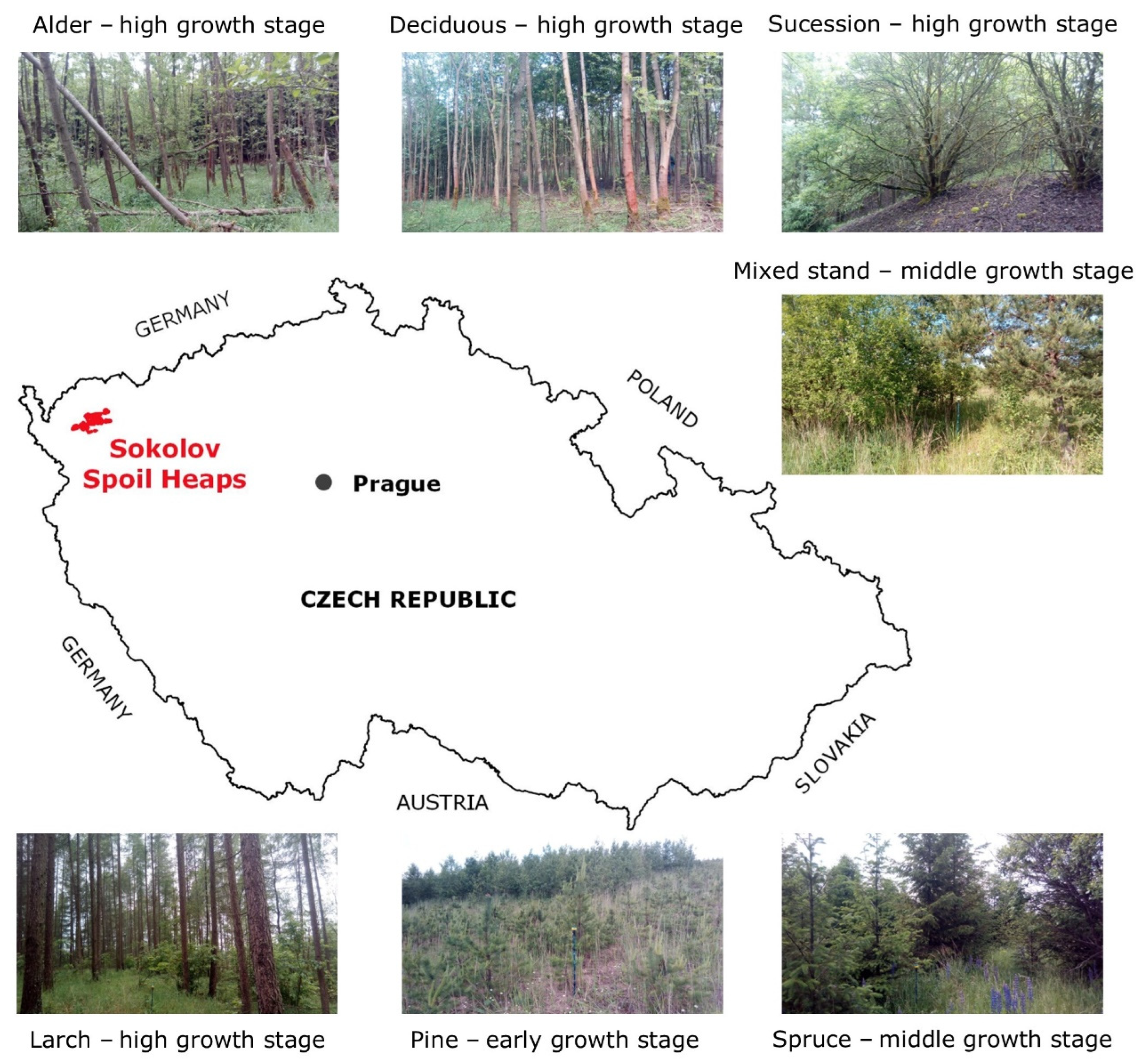
The Sokolov brown-coal mining area is situated in the western part of the Czech Republic, near the German border. The areas of interest are spoil heaps situated in the neighborhood of Sokolov town, which began to be created during the 1960s by the deposition and shaping of the overburden material excavated from up to 200 m during brown-coal open-cast mining. The geographical location of the Sokolov spoil heaps in the Czech Republic is illustrated in
Figure 1. So far, about 7000 ha of land on 10 main spoil heaps in the Sokolov mining area have been recultivated, which accounts for 75% of the area affected by coal mining there. The spoil heaps are different in size; the smallest Velký Riesl heap occupies the area of 16 ha, while the largest Velká Podkrušnohorská heap occupies 1900 ha [
35]. The geographical distribution of the Sokolov spoil heaps can be found in Braun Kohlová et al. [
19] (p. 4).
The heaps’ substrate is composed of alkaline tertiary clays—so-called cypris formation—mostly consisting of clay minerals such as illite, kaolinite, and montmorillonite; non-clay minerals such as siderite and calcite are also often present.
More than 53 thousand inhabitants live in the vicinity of the spoil heaps, namely, in three towns, including the town of Sokolov with 23 thousand inhabitants and 14 villages.
Restored forests on the spoil heaps are mainly even-aged with stands represented by one dominant tree species; there is also a mosaic of deciduous and coniferous stands, and some stands are also mixed. The restored forest stands on spoil heaps are either replanted forests with one dominant tree species or some spots are unreclaimed and left for spontaneous succession. Heaps with filled overburden were usually leveled and compacted before stands were replanted, while the terrain of unreclaimed sites was left unleveled. The surface of unreclaimed sites is characterized by numerous ridges and depressions and a series of parallel waves with a 2 m height originally created by heaping machinery during the depositing overburden on the heap [
17].
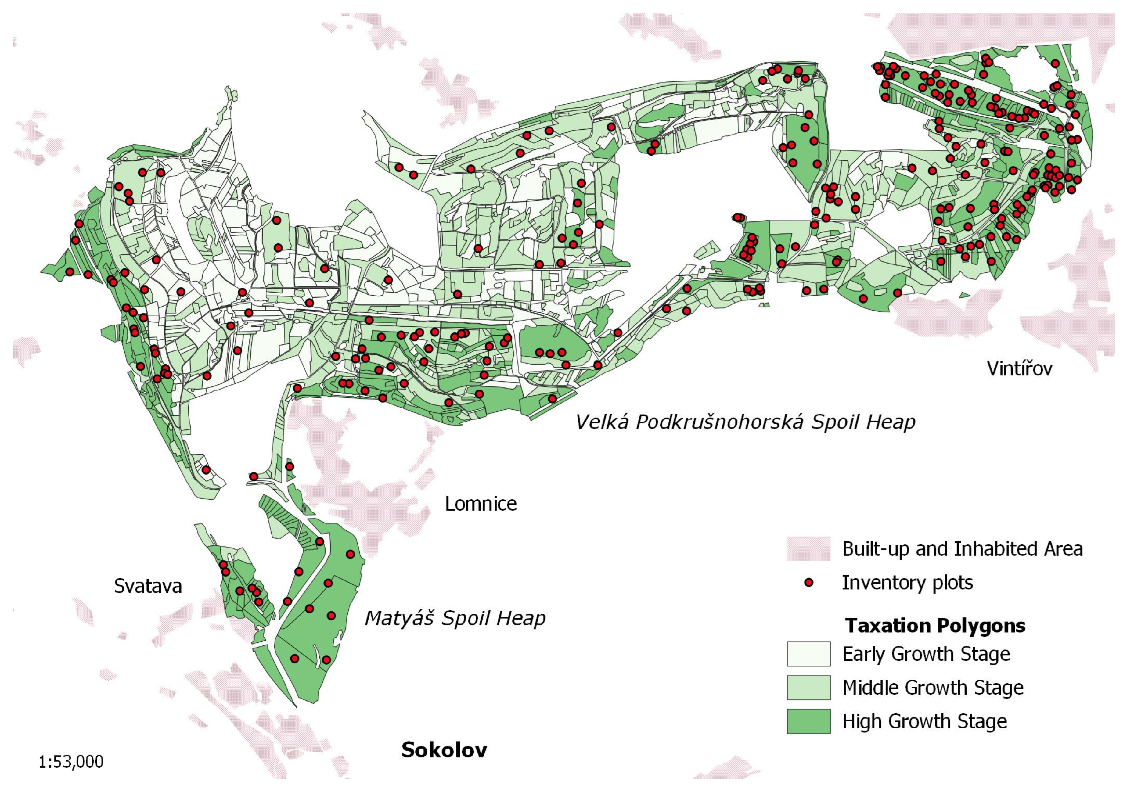
Inventory plot data [
21] measured at two Sokolov spoil heaps—Matyáš heap and Velká Podkrušnohorská heap—were used to calibrate the growth matrix model for a subsequent simulation of forest dynamics with respect to various forest restoration managements. The Matyáš heap with an area of 167 ha is the smaller one of both soil heaps, the neighboring Velká Podkrušnohorská heap—as the largest spoil heap in the Sokolov brown-coal mining district—has an area of 1939 ha and is about 10 km long and 2.5 km wide with a height up to 200 m above the original terrain. The altitude of the study site is in the range of 409–604 m a.s.l. The mean annual precipitation and temperature are 800 mm and 7 °C, respectively [
36]. The geographical distribution of the Matyáš heap and Velká Podkrušnohorská heap is shown in
Figure 2.
Replanted forest stands on the Velká Podkrušnohorská and Matyáš heap mainly consist of one tree species or two tree species of the same genus that were combined during replantation. Mostly, tree species such as Black alder (
Alnus glutinosa (L.) Gaertn.), Norway spruce (
Picea abies (L.) H. Karst.), European ash (
Fraxinus excelsior L.), Scotch pine (
Pinus sylvestris L.), European larch (
Larix decidua Mill.), European aspen (
Populus tremula L.), Austrian pine (
Pinus nigra J. F. Arnold), English oak (
Quercus robur L.), and small-leaved linden (
Tilia cordata Mill.) have been used for replanting. Silver birch (
Betula Pendula Roth) and goat willow (
Salix caprea L.) are successional trees that predominate on unreclaimed sites. The overview of the relative representation of individual tree species determined from forest inventory on the investigated spoil heaps is shown in
Table A1 in
Appendix A.
Restored forest stands growing on the Velká Podkrušnohorská and Matyáš heaps are young and middle-aged forests. Therefore, for the forest inventory purposes, we categorized these stands according to three growth stages: early growth stage with a height of up to 2 m (10–15 years old), middle growth stage of a height from 2 to 10 m (10–30 years old), and high growth stage of a height above 10 m (30–60 years old). The geographical distribution of forest stands on the Velká Podkrušnohorská and Matyáš heap corresponding to their growth stages is illustrated in
Figure 2. As prevailing stand types, stands with a dominant representation of alder, larch, pine, spruce, long-lived deciduous trees, mixed coniferous–deciduous stands, and stands with a spontaneous succession are present on the heaps (see their visualization in
Figure 1). The classification of individual tree species into the prevailing stand types is given in
Table A2 in
Appendix A.
In addition to trees, there are also shrubs and herbaceous vegetation in the stands. Among shrub species, European black elder (
Sambucus nigra L.), European hawthorn (
Crataegus oxyacantha L.) and common snowberry (
Symphoricarpos albus L.) are the most widespread species in the shrub understory of restored forest stands. Other shrub species are also present, such as wild privet (
Ligustrum vulgare L.), alder buckthorn (
Frangula alnus Mill.), dog rose (
Rosa canina L.), guelder rose (
Viburnum opulus L.), common dogwood (
Cornus sanguinea L.), Turkish hazel (
Corylus colurna L.), bird cherry (
Prunus padus L.), blackthorn (
Prunus spinosa L.), common ninebark (
Physocarpus opulifolius Maxim.), European buckthorn (
Rhamnus cathartica), and cornelian cherry (
Cornus mas L.), but their occurrence is rather rare. Most plant species, and at the same time the largest coverage of the herbaceous layer (e. g.
Festuca ovina agg.,
Pastinaca sativa,
Festuca gigantea,
Crepis biennis,
Epipactis helleborine,
Melilotus albus), are in the alder, larch, and pine stands (see [
36] for more details).
2.2. Forest Inventory Data
The matrix growth model was calibrated on data from a forest inventory survey—conducted by Cienciala et al. [
21]—with a sample of 250 inventory plots (see
Figure 2), which were randomly distributed across the Velká Podkrušnohorská and Matyáš heap. The inventory plots included restored forests, both stands established by planting and those created by spontaneous succession. In both cases, the stands were unmanaged—left to grow without appropriate forestry management since the planting or colonization with successional trees—forests until the time of inventory.
The inventory survey was planned as a single survey, i.e., with one-time dendrometric measurement on each plot. Each inventory plot was a circular plot composed of three circular zones with the following size criteria that a tree had to meet in order to be subject to a dendrometric measurement. Trees with DBH (diameter at breast height) below 7 cm and with tree height above 25 cm were measured in the zone delimited by the inner circle (radius of 2 m, area 12.6 m2). The trees above DBH > 7 cm were measured in the zone bounded by the middle cycle (radius of 5 m, area 78.5 m2) and trees above DBH > 15 cm were measured in the zone delimited by the outer circle (radius of 10 m, area 314.2 m2).
Tree and stand characteristics on the sample plots were measured throughout the year 2018. On each sample plot, the basic dendrometric measurement was taken for each individual tree that corresponded to the sampling design. Tree data collected include species, diameter, height, status (type of recruitment—natural or artificial, live, or dead standing tree), basal area, and dry matter of aboveground tree biomass. On the plot-level, stem density, natural and artificial recruitment density, total basal area, total AGB, number of tree and shrub species, total cover of shrub understory on a plot, and the age of the stand in years were derived for each plot. The list of stand characteristics and their description is provided for illustration in
Table A3 in
Appendix B.
Each plot was assigned to one of three growth phases: (i) early—stand up to a height of 1.5–2 m, (ii) middle—stand in the range of height of 2–10 m, and (iii) high—stand above 10 m in height (alder stand above 6 m in height). In addition to the growth stage differentiation, the plot was classified with respect to the seven forest stand types, i.e., according to the dominant tree species prevailing on the given inventory plot. The assignment of individual tree species to the appropriate forest type category is defined in
Table A2 in
Appendix A. Specifically, the following categories of forest types were defined—the conditions for classifying the inventory plots to the defined forest types are given in parentheses: (i) alder (alder representation of 70% and more in the stand), (ii) long-lived deciduous (≥70%), (iii) spontaneous succession (representation of succession trees >50%), (iv) larch (≥70%), (v) pine (≥70%), (vi) spruce (≥70%), and (vii) mixed coniferous–deciduous stands (if none of the above conditions are met).
While the inventory plots assigned to early and middle growth stages made up 7% and 29% of the sample, respectively, plots with trees in high growth stage accounted for 64% of the sample. The most frequent in the sample were the plots classified as mixed coniferous–deciduous, succession, and pine stand with 22%, 20%, and 15%, respectively. Plots classified as alder and long-lived deciduous stand equally accounted for 12%, plots with spruce and larch stands made up 11% and 8%, respectively.
Summary statistics of stand characteristics for plot-level variables are given in
Table A4 and mean values for other stand characteristics are presented in
Table A5 in
Appendix B. At the same time, statistics are presented for individual forest types. At the plot-level, mean tree density was highest for spruce forest stands (6300 trees∙ha
−1), the density of succession, pine, and larch stands was very similar. The mean stand recruitment was the highest for succession; this also applies for natural recruitment. Spruce stands had the highest mean artificial recruitment. Deciduous forest stands had on average the largest both basal area and aboveground tree biomass, while spruce stands had the lowest values of these stand characteristics. Deciduous stands were the oldest on average (34 years), while pine stands were the youngest (17 years). Spontaneous succession stands had the highest tree diversity on average, while alder stands had the lowest. The mean shrub species diversity was highest in deciduous stands and lowest in spruce stands. The coverage of shrub understory exceeding 22%, was measured in alder stands.
Summary statistics of tree characteristics for tree-level variables for all stands and according to forest type category are given in
Table A6 in
Appendix B. At the tree-level, succession stands had the largest mean values of DBH and aboveground biomass, while pine stands had the lowest. The average tree height was the highest for deciduous stands (14.4 m); pine stands were the lowest (8.5 m). In contrast, pine stands had the lowest mortality rate on average, while mixed coniferous–deciduous stands had the highest mortality.
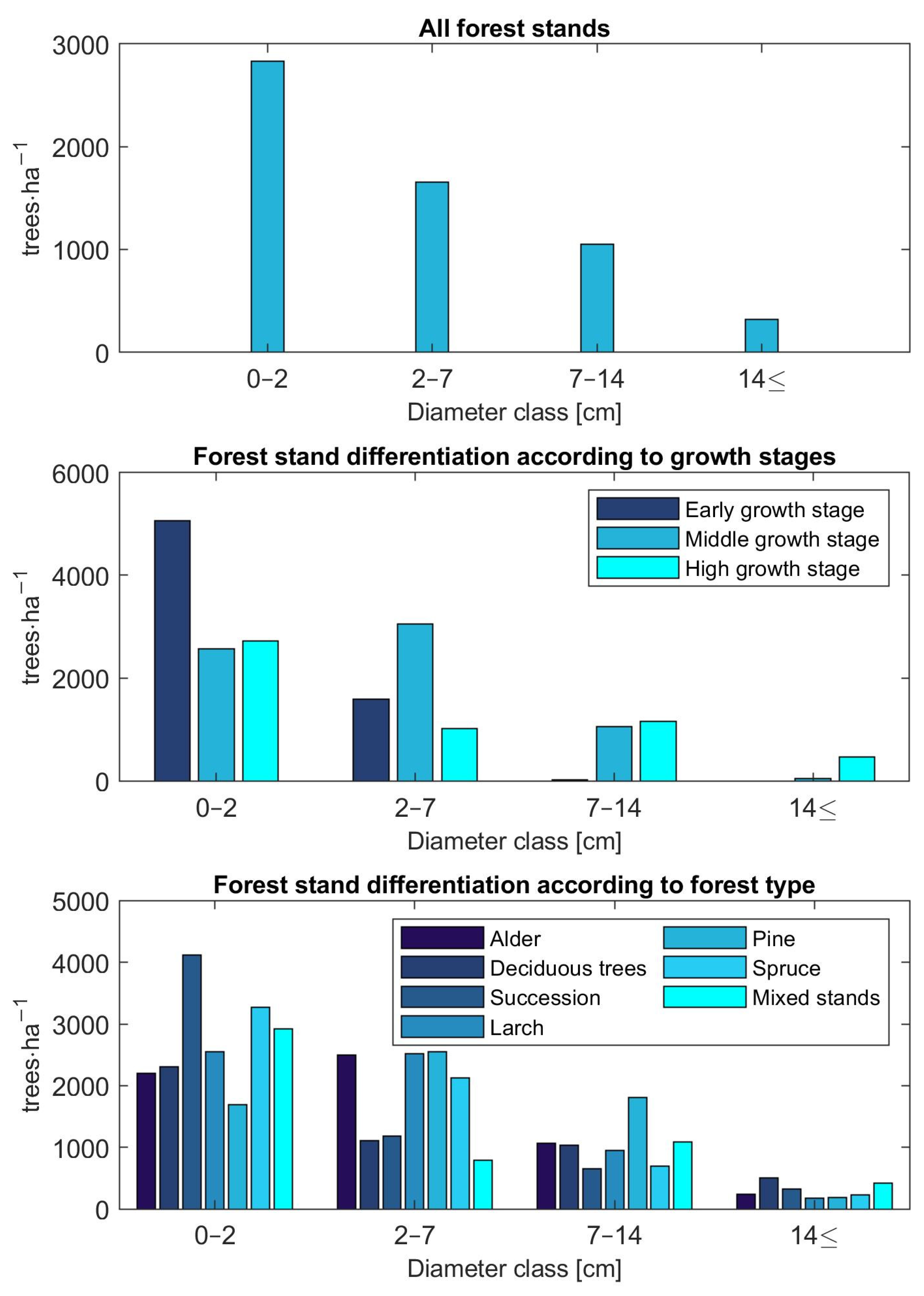
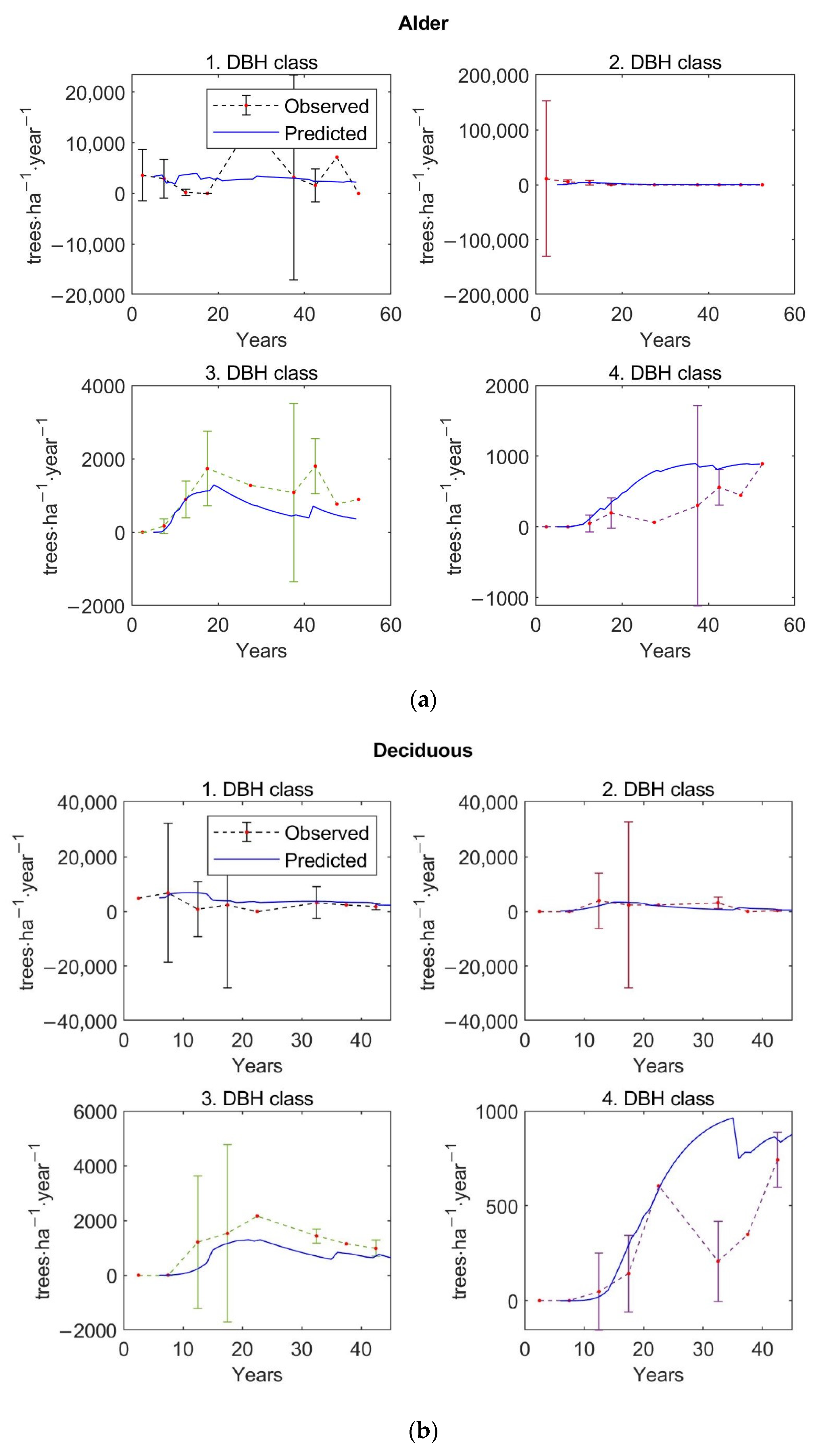
Mean values of stem density per hectare based on inventory plot data differentiated according to the DBH classes—we implemented 4 DBH classes in the growth model with the first DBH class representing recruitment: (i) 0–2 cm, (ii) 2–7 cm, (iii) 7–14 cm, and (iv) 14 cm and more—and with respect to three growth stages and seven forest types are shown in the three graphs in
Figure 3. Across all inventory plots, tree density decreases with diameter classes. Similarly, a decreasing tree density was observed for succession, deciduous, and spruce stands. In contrast, alder and pine stands reached the highest stem density in the second diameter class; larch stands had the highest density in the first two classes. Differentiation according to the growth stages shows that the stem density was the highest in the first diameter class for the early growth stage. Trees in the third and fourth DBH class are no longer observed for this growth stage. Plots of the middle growth stage reached maximum density in the second diameter class. The number of trees inventoried in the fourth DBH class was negligible for this growth stage. As with all forest stands, the distribution of tree density shows a decreasing trend for the high growth stage.
2.3. Data on Attractiveness for Recreation
Data on the recreation value of restored forest sites came from an environmental preference study [
19], in which several representative reclaimed forest stands, including spontaneous succession stands, located on spoil heaps in the Sokolov brown-coal basin were evaluated for their recreational values. The study used a discrete choice experiment (DCE), in which the participants evaluated restored stands in response to the particular photography of a given stand as perceptual stimuli. In the DCE, the measure of recreation value was represented by a person’s choice of a location with restored forests for walking in response to particular visual stimuli. The design of choice task in the DCE consisted of two hypothetical localities for recreation represented by different types of restored forest stands and a reference option of staying at home.
The survey was carried out in 2016 as an online questionnaire, which included the DCE. The resulting sample of 869 respondents consisted of the residents living in the neighborhood of spoil heaps and open-cast mines (
n = 629) and residents from the Central Bohemian region (
n = 240), which represented a control population [
19].
The questionnaire used photographs of seven forest stands representing different reclamation practices and different growth phases. Spruce, pine, and alder replantation at the age of 35 years represented the plantation practice and stands of the middle growth stage. A 15-year-old spruce replantation was also included in the DCE as the plantation of the early growth stage. Spontaneous succession as an example of an unreclaimed forest site was another type of restored forest included in the DCE and was represented by three age and growth stage classes (15, 35, 55 years, and early, middle, high growth phase, respectively).
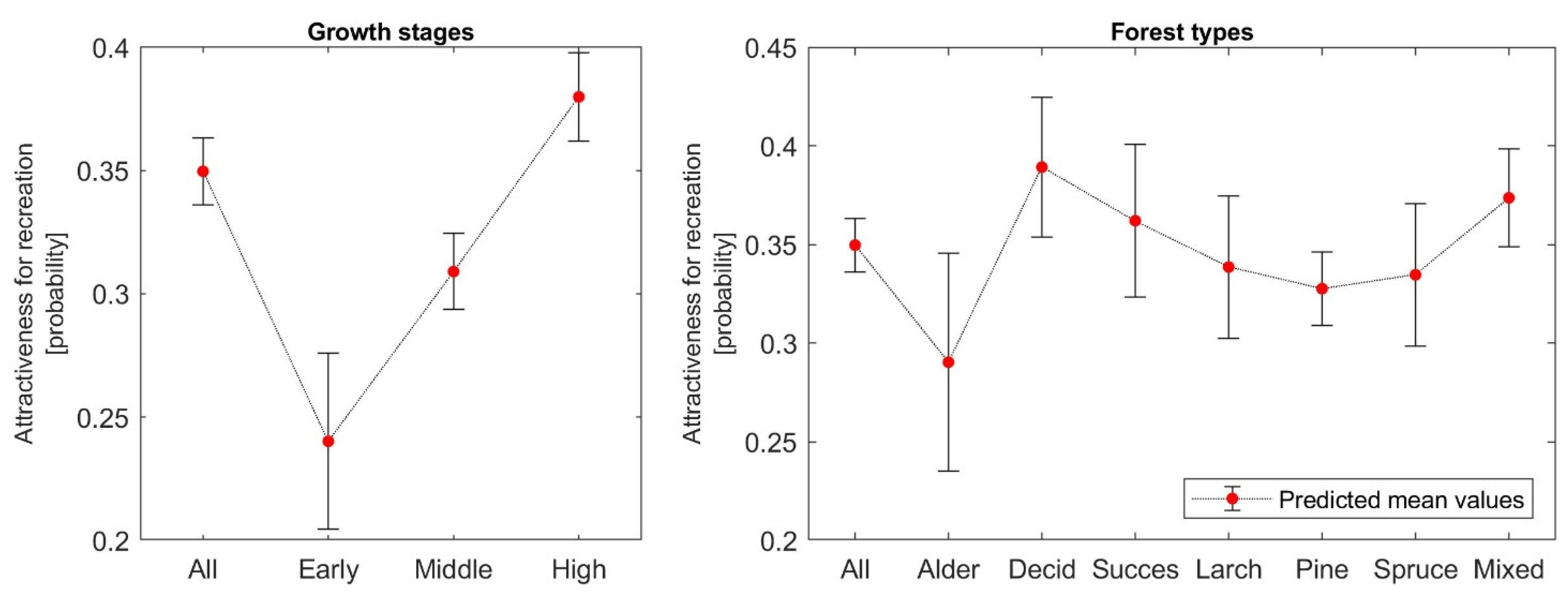
The mean recreation values—attractiveness for recreation—expressed as the mean probability of a person’s choice of a given type of restored forest for a one-hour walk are presented in
Table A5 in
Appendix B, with the highest recreation value for pine replantation and sites restored with spontaneous succession. Conversely, alder stands had a very low recreation value.
2.4. Matrix Growth Model and its Structure
The model used for the simulation of the dynamics of restored forests growing at the Sokolov spoil heaps is a density-dependent matrix growth model developed by Liang [
24]. This growth model is an extension of previous models [
30,
31] and takes into account not only harvest and natural regeneration, but also artificial recruitment. To express the dependence of the projection matrix on stand density, the tree growth, mortality, and artificial recruitment are functions of the stand basal area [
37].
In the subsequent notations, t refers to time in years (, to a type of restored forest stand, and to a diameter class. We consider the model accounting for seven types of restored forests , as they are defined in the description of forest inventory survey. Specifically, we distinguish between alder, long-lived deciduous, spontaneous succession, larch, pine, spruce, and mixed coniferous–deciduous stands. Each stand is structured into four diameter classes specified as follows: (i) 0–2 cm, (ii) 2–7 cm, (iii) 7–14 cm, and (iv) above 14 cm.
At the stand level, the state of forest according to its diametric structure is represented by a column vector
that expresses the number of live trees per hectare of restored forest type
and diameter class
at time
. The matrix growth model predicts the state of forest stand
in year
with respect to the state of forest stand
(e.g., tree density per hectare) in year
[
24,
30]. The growth model [
24] noticed in a matrix form is as follows:
where
is an Usher projection matrix or also growth matrix,
is a vector of harvest,
is a vector of natural regeneration,
is a vector of artificial recruitment, and
is a vector of random errors. The initial state of forest stand is given by a vector
.
The state-dependent growth matrix
is a block matrix:
with seven submatrices
on the main diagonal. Each block
of the growth matrix
represents the projection matrix of order 4 × 4 for a given type of restored forest stand
, where:
that describes how the trees of each restored forest type
grow or die between
and
.
The parameters and of are vital rates representing the transition probability of ingrowth and upgrowth, respectively. The parameter of ingrowth is the probability that a tree of restored forest type and diameter class survives and stays in the same diameter class j between and . The parameter of upgrowth is the probability that a tree of restored forest type and diameter class survives and grows into the diameter class between and .
Let the parameter
denote the mortality rate representing the probability that a tree of forest stand
and diameter class
dies between
and
. Then, the transition parameters
and
are related as follows:
Vector
represents natural recruitment between time
and
. Vector
is a subvector of
with zero elements except the first one
. This regeneration parameter defines the annual number of trees of restored forest type
naturally recruited in the first DBH class (0–2.0 cm) between
and
, where:
Vector
represents state-dependent artificial regeneration between time
and
. Similar to natural regeneration, vector
is a subvector of
with zero elements except the replanting parameter
in the first position. This parameter expresses the annual number of trees of restored forest type
artificially recruited in the smallest diameter class between
and
, where:
Column vector
is a harvest vector formed by subvectors
. Vector
consists of elements
representing the number of harvested alive trees per hectare for restored forest type
and diameter class
at time
:
2.5. Parametrization of Vital Rates and Projected Variables of Restored Stands
The matrix growth model (Equation (1)) is a density-dependent type of the model, of which vital rates—transition, mortality, and recruitment parameters—are dependent on the stand state , thus, the model is non-linear. The vital rates are hypothesized to be functions of stand density, respectively, stand basal area.
The vital rates were parametrized as empirical functions of tree- and stand-level variables from forest inventory data measured at the Sokolov spoil heaps [
21]. The notation of all variables is defined in
Table A3, and their summary statistics are given in
Table A4,
Table A5 and
Table A6 in
Appendix B. Both the functions of
—derived from the annual diameter growth
, see Equation (8)—and
were formulated based on individual tree-level data, together with stand-level (plot-level) data from the inventory plot in which each individual tree was growing. Conversely, the natural regeneration
and artificial recruitment
were developed as empirical functions based on stand-level data.
The aboveground tree biomass and recreation value were formulated as other empirical functions that were further used when the dynamics of restored forests were evaluated for different thinning scenarios. These functions were parametrized by stand variables—such as stand density and stand basal area—that the growth model (Equation (1)) enables us to predict. As growth rate and mortality function, the parameters of the tree biomass equation were estimated with individual tree-level data together with stand-level data. The recreation value equation was estimated with stand-level data only.
As explanatory variables, the diameter of an individual tree () and total stand basal area () were used in the annual tree diameter growth, mortality, and aboveground biomass equations. Stem density () was used in both recruitment equations to represent the seed abundance. Total stand basal area () was used in the artificial recruitment equation only. In addition to stem density, age of the dominant tree species and total cover of shrub understory () were used in the recreation value equation. Apart from tree diameter measured at the tree-level, the other explanatory variables were defined at the stand-level.
The regression parameters of all empirical functions, except mortality function, were estimated with the maximum likelihood procedure using Matlab function ‘fitnlm’. Mortality was estimated as a probit function with the generalized least squares using Matlab function ‘fitglm’.
2.5.1. Growth Function
The transition probability of upgrowth
is computed as follows [
24,
31]:
where
is the annual tree diameter growth [cm] of a tree of restored forest type
in diameter class
and in year
, and
is the width of the corresponding diameter class
[cm]. It is assumed that trees are uniformly distributed within each diameter class [
24].
The diameter growth [cm∙year
−1] is a function of tree diameter and its square (
[cm] and stand basal area, its squared and cubed form
[m
2∙ha
−1], with parameters
and error term
. The specification of non-linear diameter growth model is as follows:
According to prior biological knowledge, the tree diameter parameter
is expected to have a positive sign and
to have a negative sign. The stand basal area parameter
is expected to be negative; the parameters and of its squared and cubed term,
and
should be positive and negative, respectively. Therefore, the growth rate is supposed to increase with tree diameter, and the slower growth is expected in denser forests [
37,
38].
The total stand basal area
for each forest type
is defined at the stand-level as follows:
where
corresponds to the average basal area of trees growing in the stand of forest type
and diameter class
.
When predicting during the simulations of the matrix model, was replaced by , the midpoint of the corresponding DBH class , in Equation (9).
In the absence of permanent plot data in the study site, we used one-time plot data, the proposed method for the calculation of the yearly diameter growth
is based on the following observations and assumptions: (a) afforested forests on spoil heaps by plantation or spontaneous succession are newly formed stands on sites that previously had no tree cover; (b) the age of the stand, and thus, main trees initially planted or established by spontaneous succession, represents the time since the afforestation of the site; (c) the age of the dominant tree species that represents a given forest type
is used to determine the stand age.
Table A2 in
Appendix A shows the assignment of individual tree species to a given forest type. (d) The trees that played roles in the stand initiation are determined according to their diameter and growth phase of the stand as follows: (i) trees of the first and second DBH class of forest stands in the early growth phase, (ii) trees of the third and fourth DBH class of stands in the middle growth phase, and (iii) trees of the fourth DBH class of stands in the high growth phase.
Under these observations, the annual growth rate
of an individual tree was derived with tree-level data such as tree diameter (
) and age of the dominant tree (
) with respect to the growth phase of the inventory plot on which the tree was located. Three growth phases are classified: early, middle, and high, denoted by subindexes
,
, and
, respectively. The yearly diameter growth is calculated as follows:
where
and
are the diameter and age, respectively, of the tree of forest type
, diameter class
, and growth phase
. This means that the tree diameter growth per year is equal to DBH divided by the age of dominant tree growing on the plot. While
was computed for trees with DBH below 7 cm—1st and 2nd DBH class—for the inventory plots of the early growth phase, trees with DBH above 7 cm—3rd and 4th diameter class—and trees with DBH above 14 cm—4th diameter class—were considered when the growth rate was calculated for trees growing on the inventory plots of the middle and high growth phases, respectively.
2.5.2. Mortality Function
In the studies [
31,
32,
38] with permanent plot data, the probability of annual tree mortality is derived from the inventory records representing the state whether a tree died or remained alive between two inventories. In our study with cross-section inventory data without periodic measurement, we used the individual tree records indicating the health status of a tree. We constructed a binary variable representing tree mortality
, which equals to 1 if a standing tree of forest type
and diameter class
is dead or a standing tree is otherwise damaged, e.g., a tree with a break, and 0 if it is a live tree without visible damage. Mean values of
according to forest type are presented in
Table A6 in
Appendix B.
We used the time interval parameter
with respect to the forest type
and diameter class
to convert state-based mortality
on the probability of annual tree mortality
as follows:
The time interval parameter
is set with inventory plot age (
) as:
where
is the average age of forest stands represented by inventory plots by growth phases
and forest types
. The annual mortality rates derived from
according to Equations (12) and (13) are roughly similar to those mortality estimates obtained from the permanent plot data in other studies [
31,
38,
39].
The probability of tree mortality
is a probit function of tree diameter
, stand basal area
, its squared and cubed form
, with parameters
and error term
. The specification of mortality model is as follows:
where
is the standard normal cumulative function. The tree diameter parameter
is expected to be negative. Conversely, the stand basal area parameter
is supposed to have a positive sign, the parameters of its squared and cubed term,
and
should be negative and positive, respectively. Therefore, smaller trees are supposed to have higher mortality than larger ones, and the higher mortality rate will be in denser forest stands.
Knowing and , the transition probability of ingrowth is computed according to the relation in Equation (4).
2.5.3. Recruitment Functions
Dissimilar to growth rate and mortality, both natural regeneration and artificial recruitment,
and
[trees∙ha
−1∙year
−1], are developed as stand-based functions, and they are specified as linear functions of stand density,
[trees∙ha
−1∙year
−1]. Specifically, natural regeneration is a function of stand density with parameter
and error term
, and has the following form:
The stand density parameter is expected to have a positive sign, so that more trees increase the abundance of seeds and cause a higher rate of regeneration.
Artificial recruitment is a function of stand density and stand basal area, with parameters
and error term
and has the following specification:
One would expect both parameters of stand density and stand basal area to be negative. Therefore, a smaller number of trees in the stand would require a higher intensity of artificial planting. However, the larger the stand basal area is, and thus, stand density, the higher the competition between trees will be.
Data for the recruitment,
and
, i.e., the number of trees per hectare entering yearly the smallest diameter class as natural regeneration and artificial planting, respectively, were computed from the inventory data measured on individual trees of up to 2.0 cm DBH. First, a tree from recruitment was assigned to either (1) the natural or (2) the artificial recruitment category
based on the regeneration origin determined during the inventory survey. Furthermore, the average annual height increment of recruitment (
) for each restored forest type
was derived with tree-level data such as tree height (
) and age of the dominant tree (
) measured on inventory plots of the early growth phase—trees up to 2 m height—as follows:
where
and
are the tree height and age, respectively, of the average tree of forest type
, diameter class
, and growth phase
. The annual height increment of recruitments was from 9 cm for deciduous, larch, and mixed stands to 28 cm for succession stands. The height increment of spruce, pine, and alder stands amounted to 15 cm, 18 cm, and 24 cm, respectively.
The parameter
was then used to measure the annual recruitment
—both natural
and artificial recruitment
—on each inventory plot as follows:
where
and
are, respectively, the tree height of the average tree and the number of trees of forest type
, diameter class
, and recruitment type
, on a given plot.
2.5.4. Function of Aboveground Tree Biomass
The volume of aboveground tree biomass of individual trees
[tonnes∙tree
−1] is a function of tree diameter
, stand basal area
, its squared and cubed form
, with parameters
and error term
. The specification of tree biomass model is as follows:
Since the tree volume is related to the tree diameter, the parameter should be positive. The stand basal area reflects possible effect of stand density, so that tree volume should be higher in a less dense stand. Therefore, the stand basal area parameter is expected to be negative, the parameters of its squared and cubed term, and , should be positive and negative, respectively.
The data for
in Equation (19) were determined using the allometric equations, which were predominantly derived for main tree species and different tree components in the central Europe [
40,
41,
42,
43,
44,
45,
46,
47]. Specifically, the calculation of aboveground tree biomass consisted of deriving the volume of following tree component: coarse wood (≥7 cm in diameter), bark of coarse wood, small wood (<7 cm in diameter) including bar, and needles (in conifers). Individual tree inventory data such as DBH and tree height were used as explanatory variables in the component biomass functions.
2.5.5. Function of Attractiveness for Recreation
The recreation value
[probability] as attractiveness of restored forest stands for recreation, is a function of the proportion of stem density (
) to age of the dominant tree species
, and total cover of shrub understory
, with parameters
and error term
The model on recreation value is specified as linear-log model:
The shrub understory parameter
is supposed to have a negative sign, so that shrubs detract from scenic beauty of forest stands, as found by Brown and Daniel [
48]. The parameter
is assumed to be negative, since increasing stand age should have positive scenic impact, thus, increasing recreation value of the stand. The effect of tree density on recreation value is opposite. As found by Hull et al. [
49], the age of stand has a positive effect on scenic beauty, but in interaction with tree density, since increasing density weakens the age effect.
The parameters of the recreation value model were estimated with forest inventory data [
21] and with the estimates of recreation value derived in the environmental preference study [
19]. The data for recreation value,
in Equation (20), were represented by mean recreation values predicted by the DCE model for seven restored forest stands at the Sokolov spoil heaps in the environmental preference study. Forest inventory data—such as tree density, age of stand, shrub coverage—from seven inventory plots geographically corresponding to the restored forest stands, where photographs were taken in 2016 for the assessment of the attractiveness for recreation in the environmental preference study, was subsequently attached to the data on recreation value.
2.6. Verification of the Growth Model
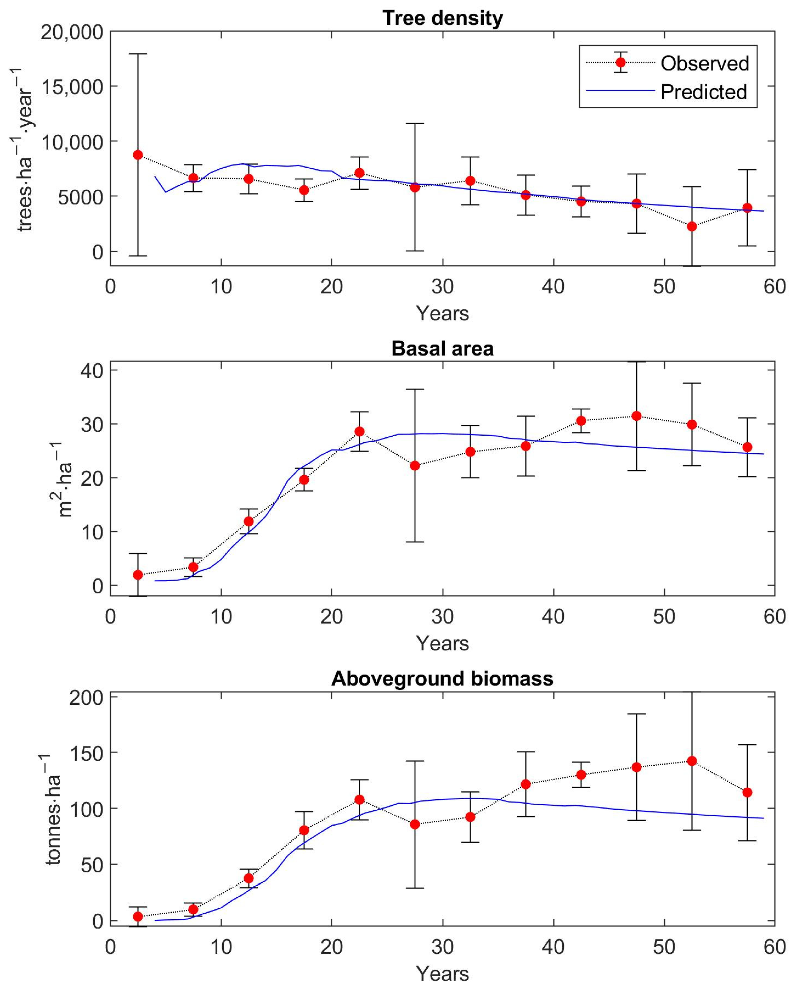
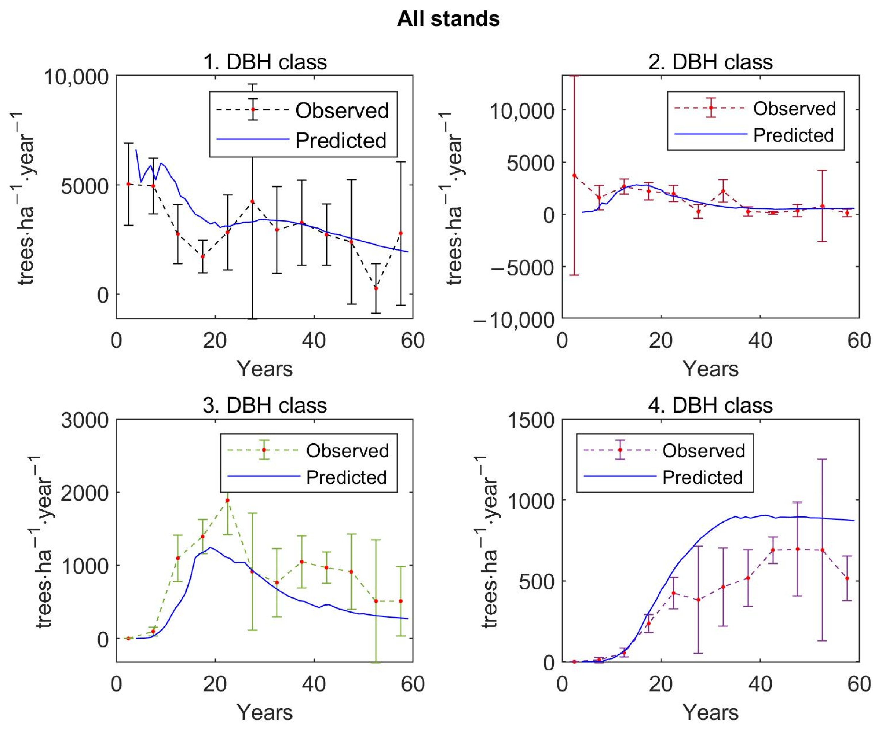
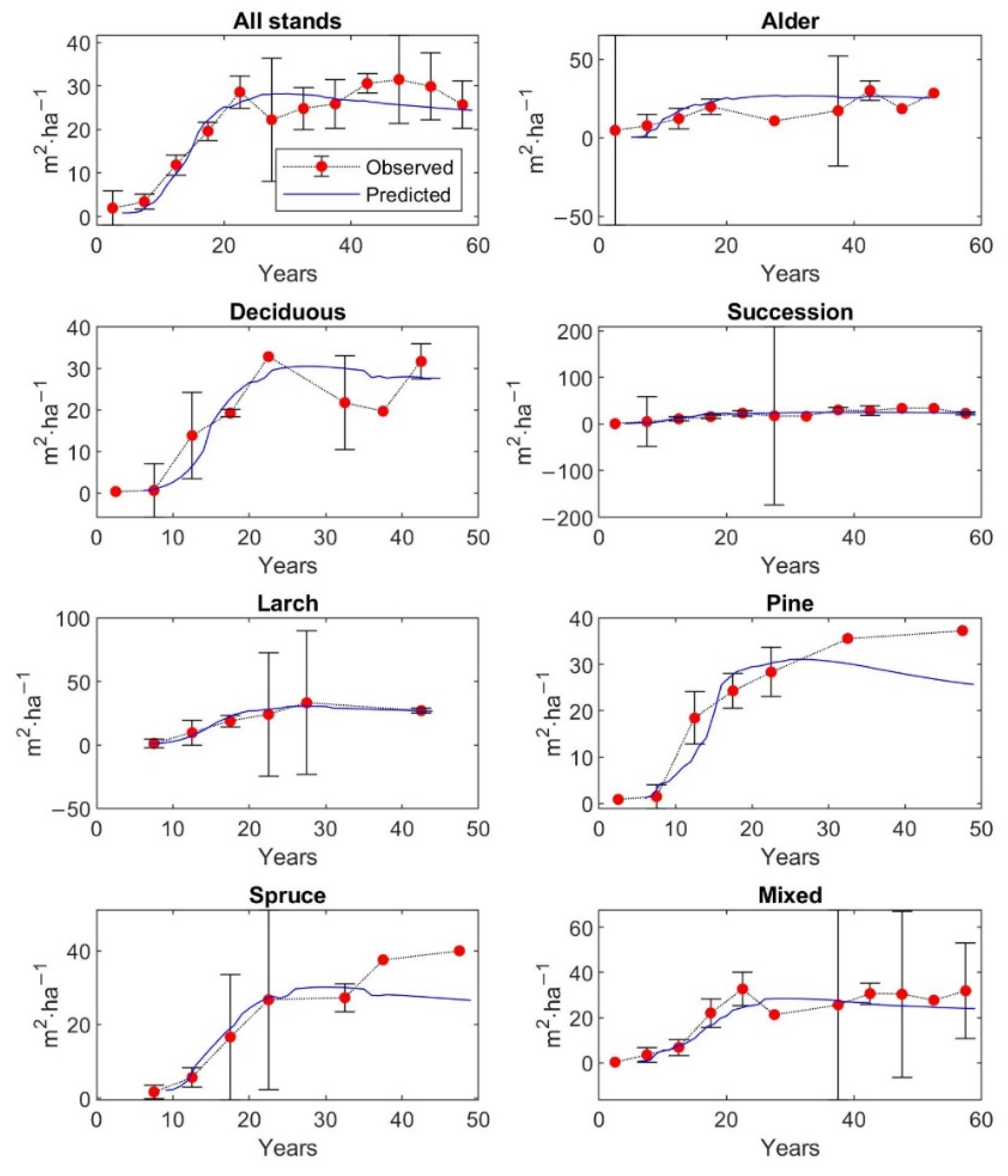
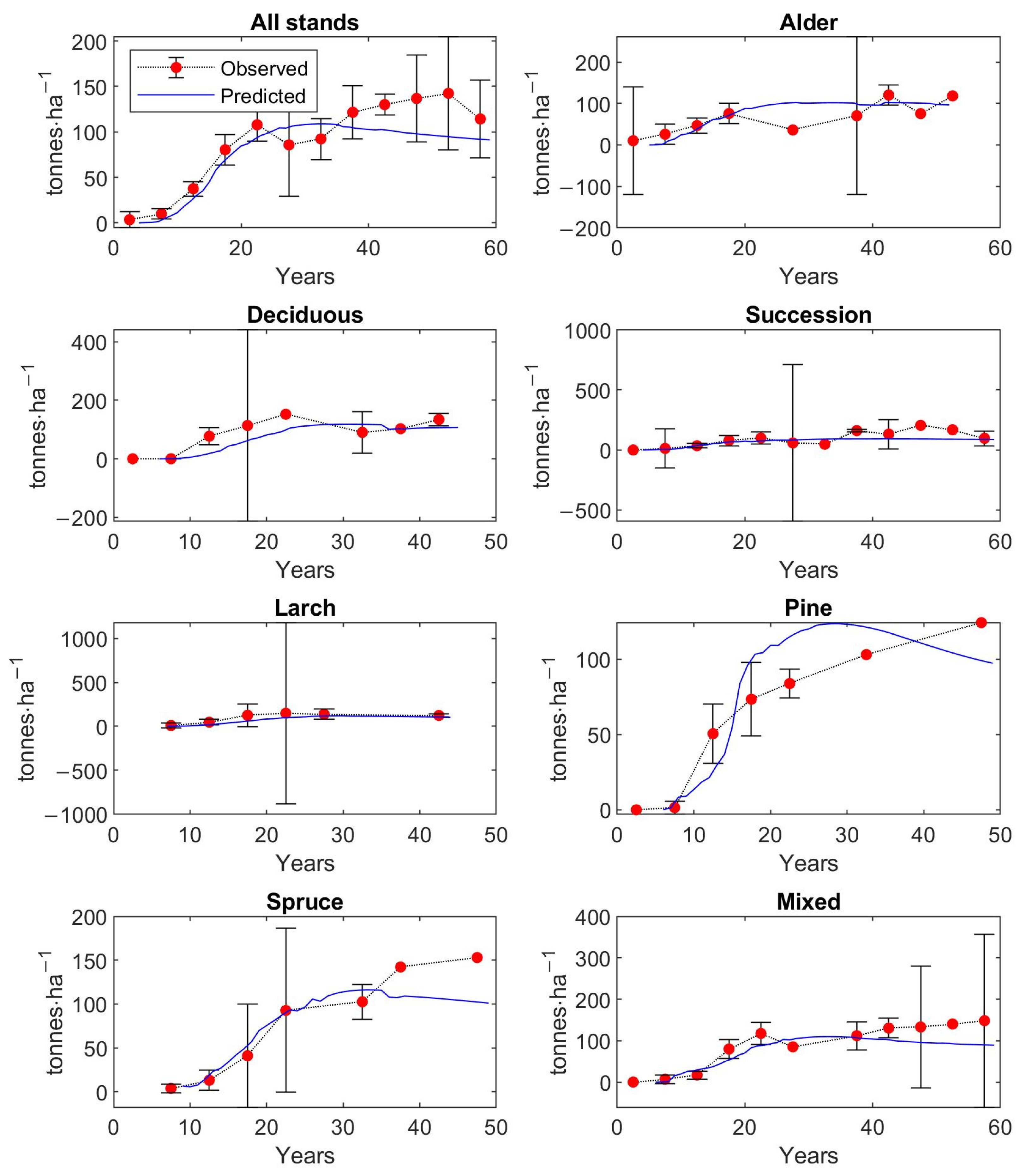
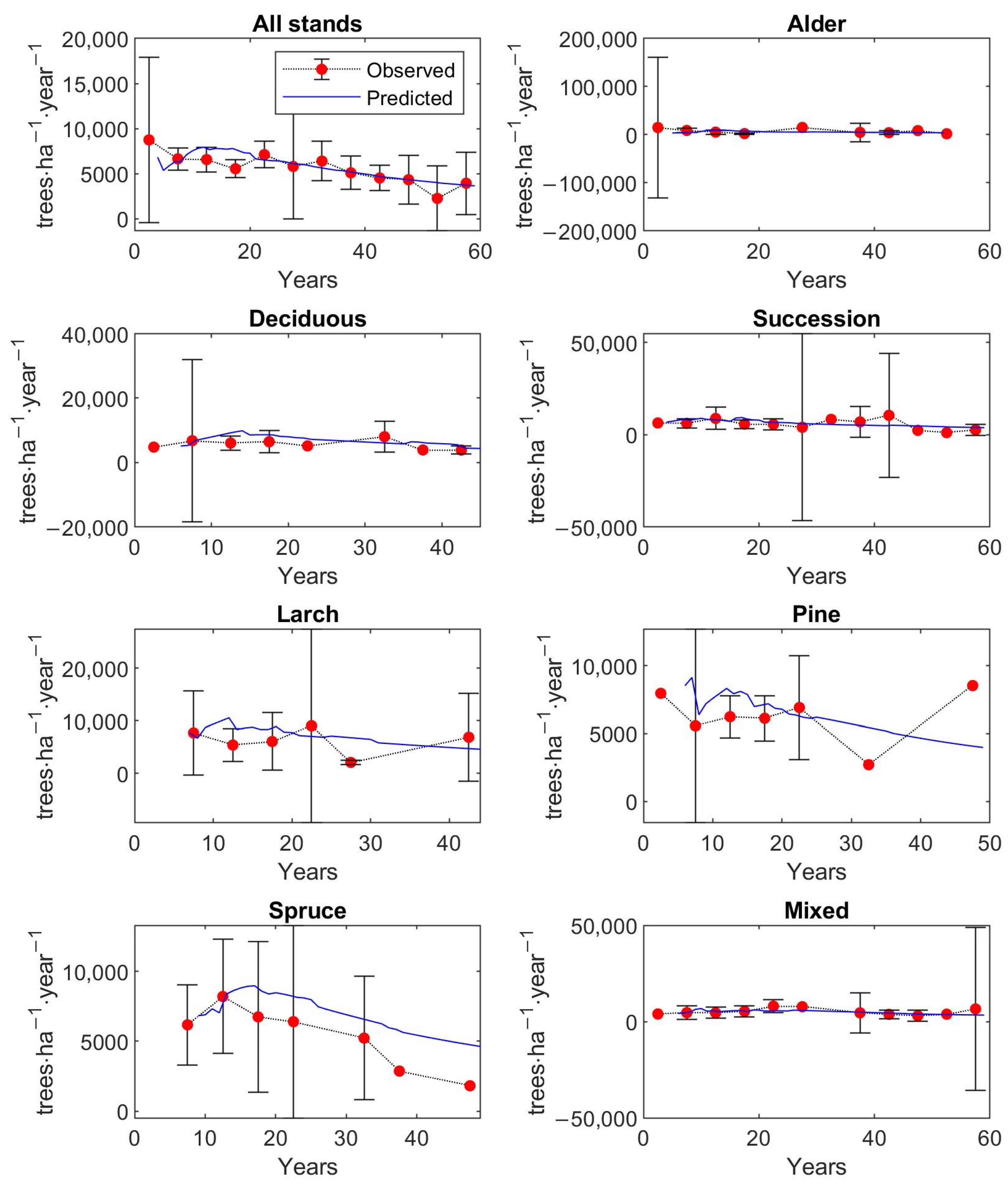
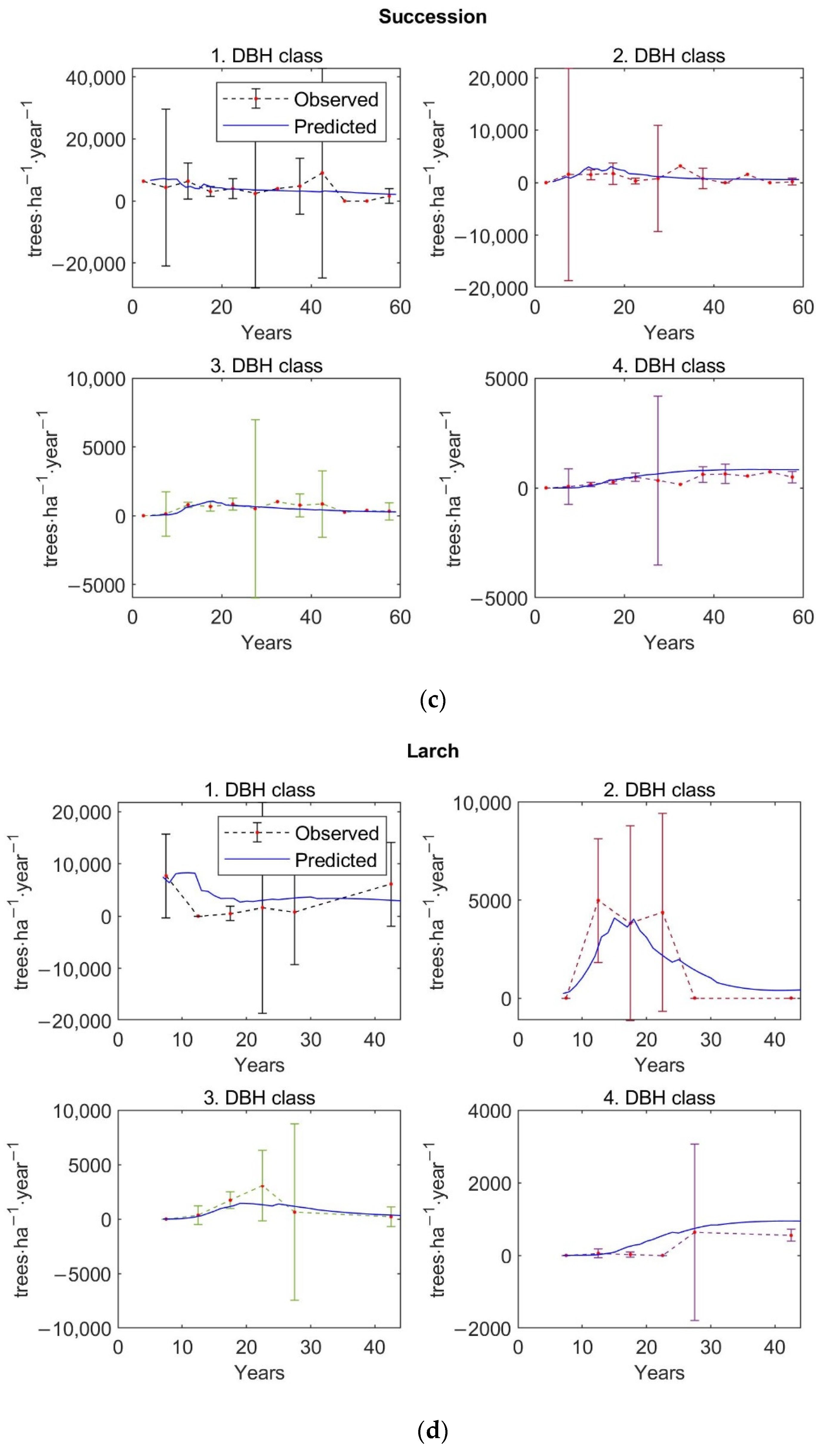
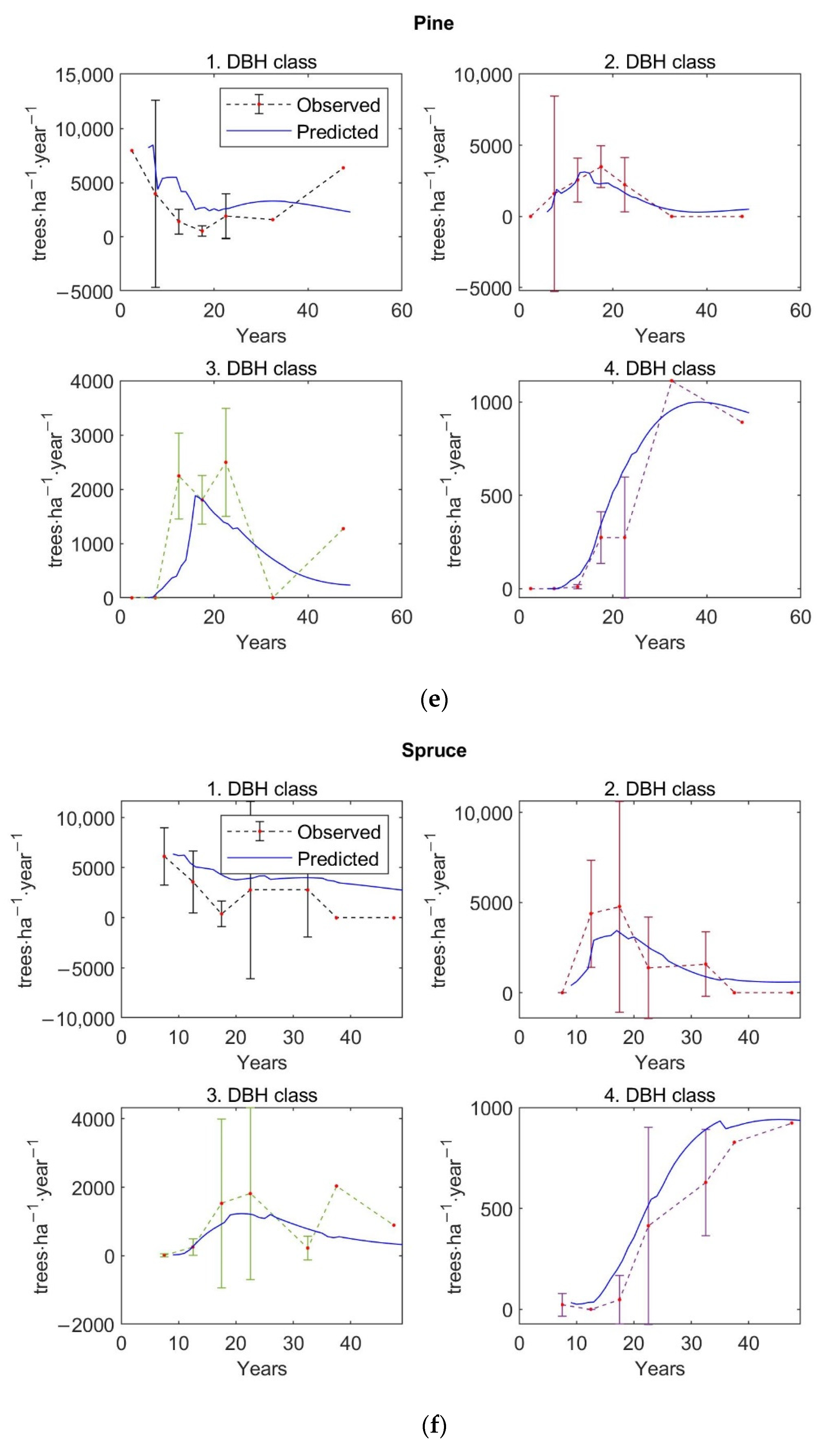
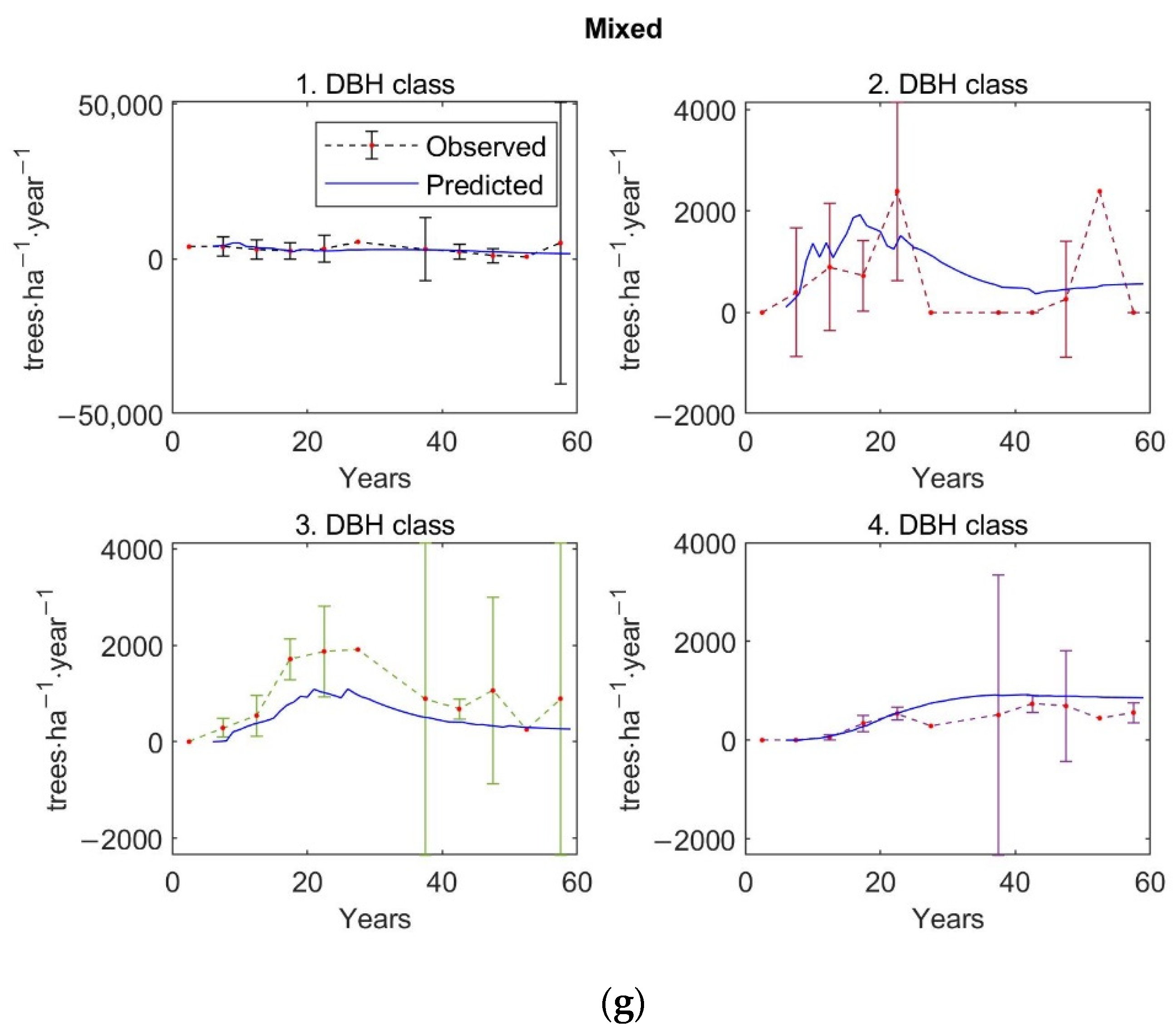
The matrix growth model (Equation (1)) with empirical functions (Equations (9), (14)–(16), (19)) representing individual variables in the matrix model was calibrated on inventory plot data from the Velká Podkrušnohorská and Matyáš heap. Verification—accuracy of the calibrated growth model was determined based on the prediction errors, the differences between the observed values of stand characteristics—stem density, density according to the DBH classes, basal area, and AGB—and the predicted values of these simulated forest characteristics.
The observed values of stand characteristics were expressed as 5-year averages. In the given 5-year average, only those inventory plots whose age was within the given 5-year interval were included. At the same time, a 95% confidence interval was determined with the 5-year average of the observed forest characteristic.
The accuracy of the model was verified on 250 inventory plots. The growth model was used to simulate the dynamics of restored forest stands on each inventory plot in a one-year time step up to the age of 59 years. This age corresponds to the maximum age that was determined during the forest inventory survey for the dominant tree growing on the inventory plot. The initial state of forest stand used for simulation corresponds to the observed state of the restored forest on the given inventory plot.
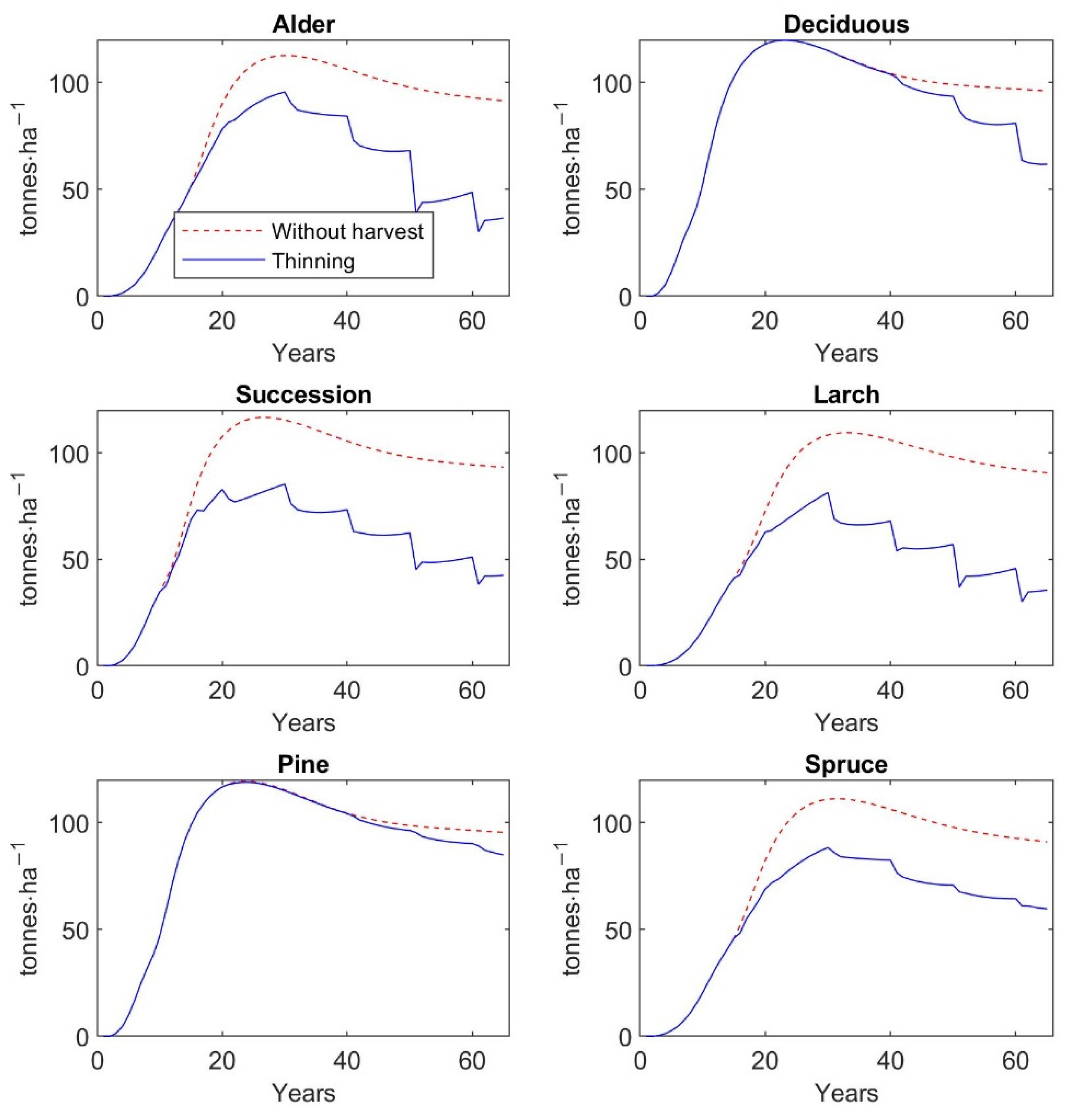
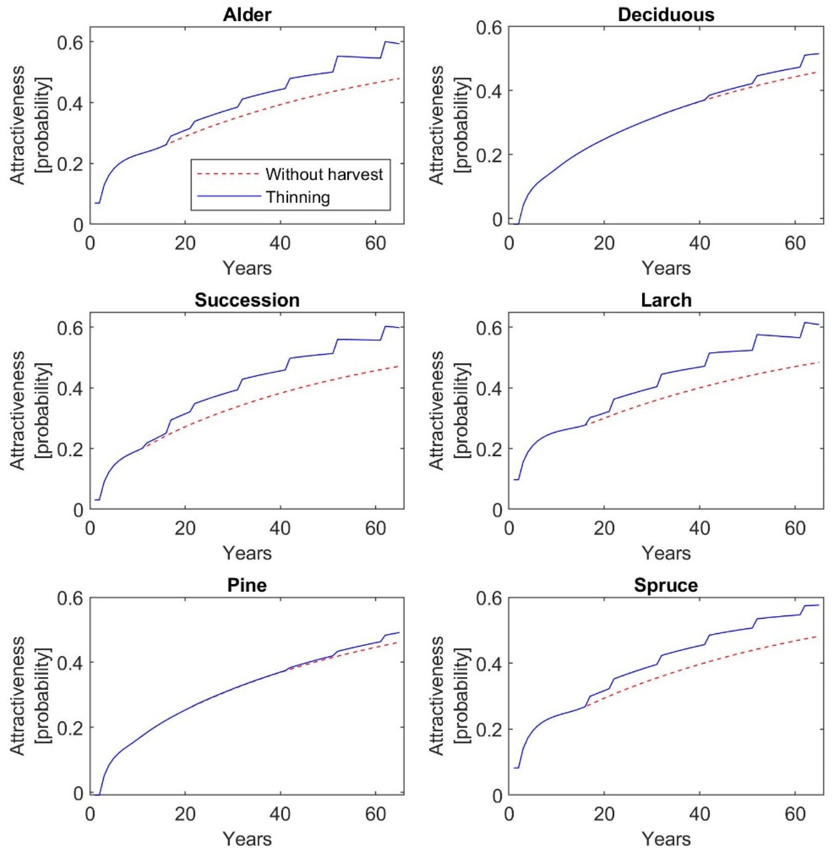
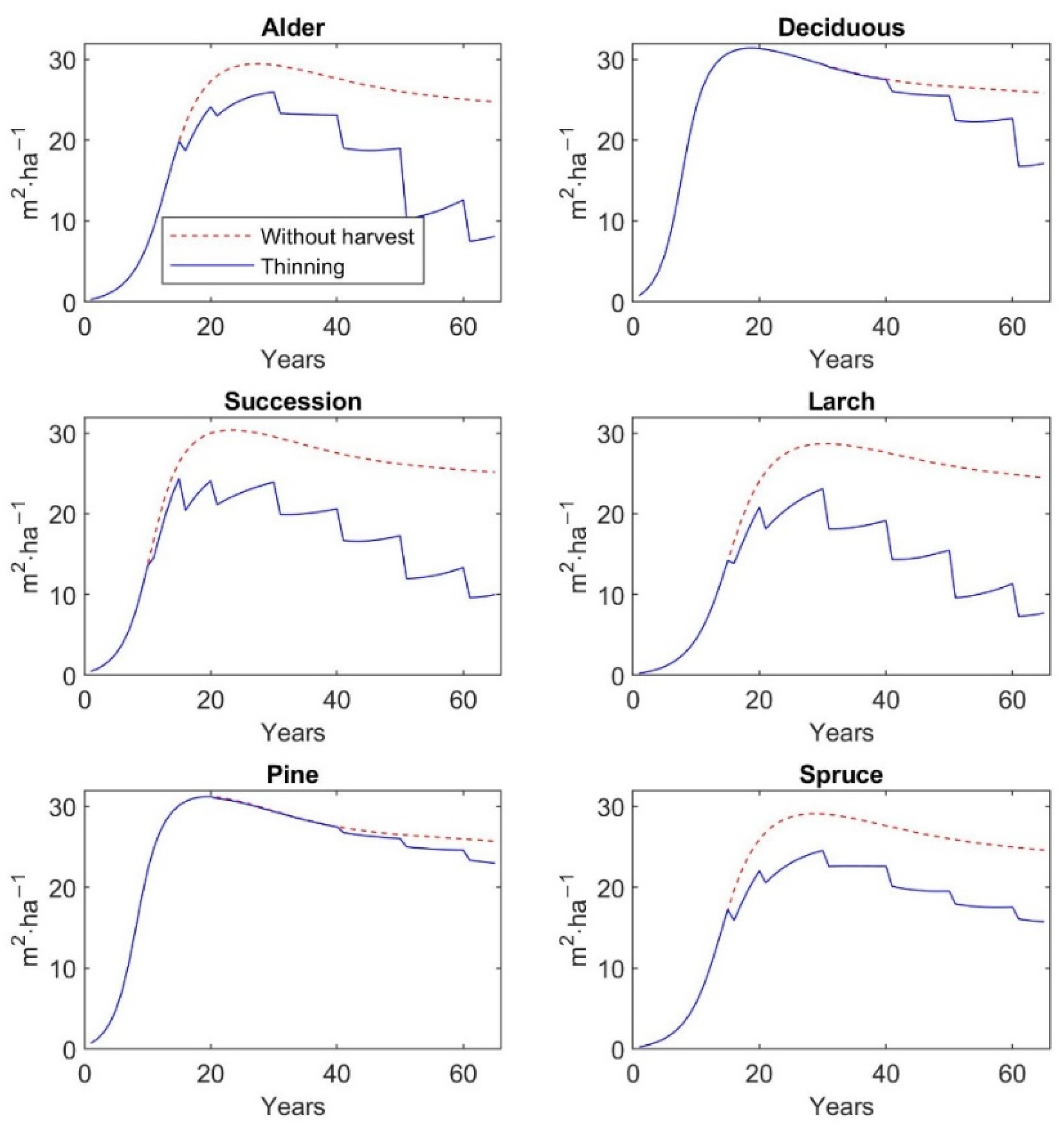
2.7. Application of the Model to Differenct Thinning Managements
The matrix growth model calibrated on inventory plot data from the Sokolov spoil heaps—Velká Podkrušnohorská and Matyáš heap—was applied to study the dynamics of six types of restored forests—alder, deciduous, successional, larch, pine, and spruce stands—with and without the management of various regimes of thinning. The simulation was mainly focused on the prediction of the recreation value and aboveground biomass under different thinning regimes, which correspond to a given type of restored forest stand. The simulation was run in a one-year time step for each thinning scenario for 65 years with a 5-year cutting cycle up to 20 years of stand age and a 10-year cutting cycle in the rest of the simulated period. The simulation period up to 65 years represents the age range of restored forests of early, middle, and high growth stage that are present in the study site. Older restored stands are absent in the Sokolov mining area, because the first forest reclamations were started here only at the beginning of the 1970s.
The parameters of thinning measures considered in the simulation are based on the framework guidelines for the management of reclaimed forests [
50], which were drawn up for the Sokolov spoil heaps within this study. For each stand type and age, the guidelines propose the state of the forest stand, which corresponds to the minimum target numbers of trees per hectare after thinning in a given cutting year. The minimum target numbers of trees per hectare are given in
Table A7 in
Appendix C.
4. Discussion
Following the findings of previous studies [
18,
19], the results have shown that restored forest stands—both replanted and sites with succession—at the Velká Podkrušnohorská and Matyáš spoil heaps in the Sokolov brown-coal mining area, which are left to grow without appropriate silvicultural management, have a lower recreation value than forest stands with targeted after-care such as thinning and pruning. This is consistent with the findings of the study on perceived beauty of various restored forest stands in the North-West Bohemian brown-coal basin in the Czech Republic realized by Sklenicka and Molnarova [
51], in which managed coniferous forest received higher preferences than wild, unmanaged, deciduous forest. On the other hand, the wilderness element of the forest landscape was not significant in the study by Svobodova et al. [
52], in which visual preferences of different type of restored landscape were evaluated in the same brown-coal district as in the previous study.
In the matrix growth model (Equation (1)), the recreation value of the restored forests is parametrized apart from the stand age and shrub cover by tree density (Equation (20)) with its negative effect on recreation value, when the decreasing tree density increases the attractiveness of reclaimed forests for recreation. The tree density effect reflects well the stand conditions after the thinning selections in the long-term horizon when the direct remnants of logging are no longer visible. However, the model does not reflect the short-term post-thinning stand conditions, with slash piles, small diameter downed wood, and other visible harvest effects detracting from the scenic beauty and recreation value of managed stands [
48].
In addition to the tree density, the results indicate that the recreation value of restored forests increases with the age of the stand. The positive effect of stand age on the attractiveness of reclaimed forests for recreation or on their perceived beauty was previously confirmed by Braun Kohlová et al. [
18,
19], and Sklenicka and Molnarova [
51], respectively, for restored forest sites in the Sokolov and North-Bohemian mining area. This means that the restored forest stands of an early (<2 m) and middle (2–10 m) growth stage are characterized by low recreation value; this was confirmed for both successional stands [
18,
19] and replantations [
52]. Interestingly, the significantly lower recreation value of early-stage restored stands was observed for spruce plantation compared to spontaneous succession [
19]. This can be explained by a lower density of successional stands in their initial phase, while the spruce is planted in high seedling densities (10,000 seedlings per hectare).
The level of shrub and herbaceous understory and ground deformations are among other stand-level attributes that affect peoples’ preferences towards recreation in restored forests. While the effect of shrubs—the presence of shrub layer detracts from visual attractivity of restored stands—was taken into account in the model on recreation value (Equation (20)), the cover of the herbaceous understory was not measured on the inventory plots, and therefore, the presence of herbaceous vegetation was not considered in the model. This may result in higher estimates of the recreation value of restored stands, especially those with a thick herbaceous vegetation. This is particularly problematic in alder stands with a high fixation of natural nitrogen that supports the spreading of grasses such as
Calamagrostis epigejos or
Arrhenatherum elatius [
36]. It was alder stands with a large understory vegetation of
C. epigejos that were perceived as less attractive than other restored forest stands [
18].
Ground deformations caused by the conveyor belt dumping and layering of overburden material into 1–2 m high waves during the technical reclamation of the spoil heap are a suitable place for the development of spontaneously emerging ecosystems and the growth of succession tree species [
10,
17]. However, visible ground unevenness present at unreclaimed places left to spontaneous succession detract from the attractiveness of successional stands for recreation, as proven by Braun Kohlová et al. [
18]. The highest growth phase of succession (
B. pendula) was perceived as more attractive than the early (
B. Pendula,
P. sylvestris,
P. abies) or middle (
S. caprea) growth phases. In part, this may be influenced by less visible geomorphological irregularities in high growth stage stands due to geophysical processes. This might partially overestimate the predicted recreation value of successional forests in their early and middle growth stages.
From the long-term perspective, we can, therefore, recommend the formation of numerous ridges and depressions when a spoil heap is created, supporting the emergence and growth of successional forests. At suitable places on the spoil heap, strongly deformed terrain with spontaneous succession can be carefully combined with a phytotoxic surface. This will create future open areas with scenic landscape views and a habitat for rare plant species [
10]. Deeper deformities give birth to ponds and pools suitable for amphibians. After opening these locations with spontaneous succession to visitors, we can inform the public about the importance of habitats for biodiversity and its origins. This information can take many forms, such as information boards or natural trails.
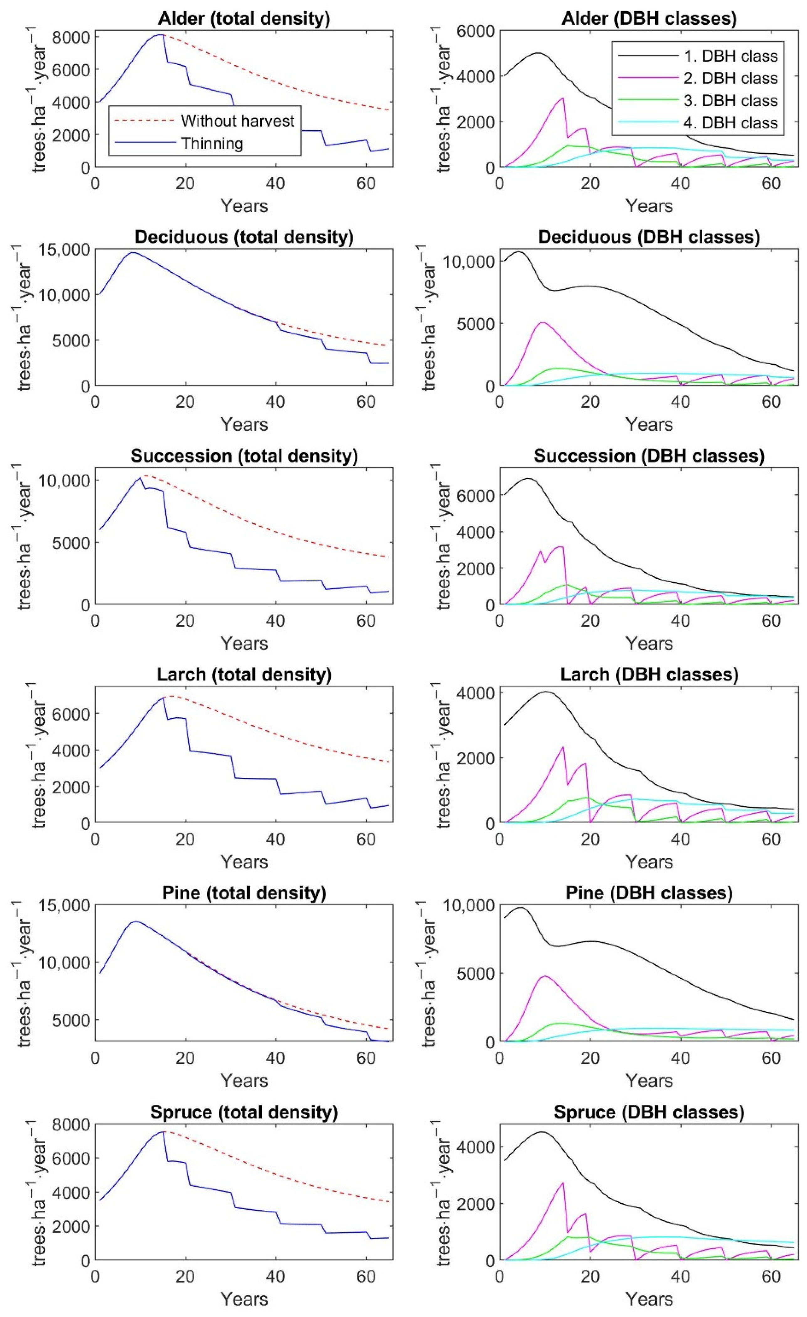
Furthermore, the findings of the current study indicate that thinning of different intensities increases the recreation value of restored forests, but at the same time the aboveground tree biomass significantly decreases, except on pine plantations. AGB and recreation value—measured as mean probability of a person’s choice of a given forest type for a one-hour walk—of a 65-year-old pine stand is 84.9 t∙ha−1 and 0.49, if thinning management is regularly realized. On the other hand, larch plantations at the same age reach 35.6 t∙ha−1 AGB, but recreation value amounts to 0.61. In comparison to unmanaged stands, the AGB of 65-year-old larch stands due to thinning operations is decreased by 61%, while recreation value is increased by 26%. The similar values and dynamics in AGB and recreation value as for larch stands are observed for alder plantations. Deciduous and spruce stands at the age of 65 reach 61.8 and 59.2 t∙ha−1 AGB, and their recreation value is 0.52 and 0.58, respectively. The regular thinning and, thus, subsequent decrease in AGB by 35% in both types of plantations will increase recreation value by 12% for deciduous stands and by as much as 20% for spruce stands. The highest increase in recreation value by 27% is observed for successional stands, which is accompanied by a 54% decrease in AGB. A 65-year-old successional stand reaches 42.5 t∙ha−1 AGB with recreation value at 0.60.
From the timber production perspective of the individual forest types of restored stands, pine forests (usually
P. sylvestris or
P. nigra) created by plantation have an above-average wood yield, especially if the thinning interventions are regularly realized in the middle and high growth phase. This is consistent with the findings of the study by Vacek et al. [
53], which proved high productivity and stand volume of
P. sylvestris on the reclaimed forest site at the Antonín spoil heap in the Sokolov mining area, even though the pine restored stand was insufficiently thinned out. At the same time,
P. sylvestris was found to be very adaptive towards climate change. However, pine forests have worse pedogenetic characteristics than alder or succession forests, as confirmed by Melichar et al. [
54] at the Velká Podkrušnohorská and Matyáš spoil heaps.
The successional forests have an average wood yield, as was also confirmed by Vacek et al. [
55] at the Antonín spoil heap. The mean stand volume of successional stands (
Populus tremula,
S. caprea, or
B. pendula) were significantly lower than on afforested stands by
Q. robur,
B. pendula, or
Alnus glutinosa. However, the reclaimed sites colonized with successional trees are significant for their pedogenetic process and tree and herbaceous diversity [
54]. The higher species richness and total stand diversity of successional sites compared to replanted stands were also proven by Vacek et al. [
55] for the Antonín heap.
Forest plantations predominantly with alder have a lower-than-average wood yield; wood volume per hectare is less than for successional forests. This was confirmed at the Velká Podkrušnohorská heap by Frouz et al. [
56], when woody biomass was significantly greater on successional sites (
P. tremula and
S. caprea) than on replanted sites by
A. glutinosa at their high growth stages. Nevertheless, woody biomass was greater for alder stands than for successional sites at their early and middle growth stages. The stand volume of alder plantation at the high growth stage was also lower compared to replanted stands with
Q. robur and
B. pendula and the successional stand with
P. tremula at the Antonín heap [
55]. However, successional forests with
S. caprea, or
B. pendula had a lower stand volume than the alder plantation. Nonetheless, alder planting at spoil heaps is mainly motivated by its suitability as a preparatory tree species. The pedogenetic role of alder stands is crucial, even though natural conditions on soil heaps are less favorable for alders and, thus, cause its premature aging [
54]. The species diversity of alder stands is also relatively high compared to spruce, pine, long-term deciduous, or silver birch plantations [
36,
55].
One of the limitations of the matrix growth model is the fact that the model is calibrated on the inventory data of the restored forests from early to high growth stage up to the age of 60 years at maximum, because older forest reclamations are absent in the Sokolov mining area and also in other coal mining areas in the Czech Republic. Therefore, we have used the model to simulate the forest dynamics and evaluate the effects of the thinning interventions for a period of 65 years. Beyond this time horizon, we would not be able to evaluate the errors between the predicted and actual stand states. The possible improvement of the model would be to establish the inventory system of permanent plots capturing a wide range of restored forest types, soil, and geomorphological conditions in the study site and to extend the simulation period beyond the current time horizon of 65 years. In addition, the vital rates including the diameter growth, mortality, and both artificial and natural recruitment rates were parametrized with one-time inventory plot data. Second forest inventory with dendrometric measurements on the same inventory plots as in 2018 could greatly enhance the validity of the estimated parameters of the matrix growth model (Equation (1)).
Finally, in addition to the biomass production and recreation function, the restored forest ecosystems positively influence the properties of reclaimed soil, store carbon in AGB and in soil organic matter, and create the habitat conditions favoring herbaceous species diversity. Given the availability of data from pedological and phytocenological surveys [
36,
57] realized at the Sokolov spoil heaps in recent past, the opportunity exists to further extend the matrix model with the soil properties, carbon storage, tree and herbaceous diversity, and to study the stand dynamics from the perspective of the multifunctional use of restored forest ecosystems.


 ,
, 


