Fuel and Time Consumption in Alpine Cable Yarder Operations

Abstract

A survey was conducted on 12 cable yarding operations in northern Italy, with the purpose of determining fuel consumption and time use. The observation unit was the individual operation, intended as all the activities needed to complete the harvesting of a sale (mean = 500 m³ of timber). All teams were equipped with a tower yarder, an excavator-based loader or processor and a truck or a tractor with trailer, if intermediate transportation to a larger roadside landing (two-staging) was required. The crew size was 3 or 4 operators. Time and fuel use were recorded separately for the following tasks: relocation; set up & dismantle; commuting; yarding; processing and/or loading; major delay events. Fuel consumption averaged 5.1 L m⁻³, of which 2.2 L m⁻³ was incurred by two-staging. In general, the yarder accounted for less than half the total fuel consumption of the operation: the processor was indeed the main consumer. Relocation had a very small incidence on time and fuel use. Set up and dismantle did not incur significant fuel consumption but occupied a meaningful share of total time (mean = 22%). Commuting also incurred unexpectedly large (and generally neglected) fuel and time use—with means at 13% and 7%, respectively. Technology developments aimed at reducing fuel consumption should target both main consumers: the yarder as well as the excavator-based processor. Significant benefits would also be achieved through improved planning and infrastructure development, aimed at minimizing the need for intermediate transportation (i.e. two-staging).

1. Introduction

The adjective “unprecedented” has come into popular use following the recent Covid pandemics and it is now used (and abused) to describe a wide variety of new and shocking events. However, it would be hard to use it for the latest energy crisis caused by the Ukrainian conflict. Recurrent fuel shortages represent the structural problem of a global economy that keeps growing faster than the resources it needs for further expansion. That is true for all activities, including forestry. Large amounts of fuel are used for such activities as stand establishment, tree tending and wood harvesting. Among those activities, wood harvesting is the largest user of diesel fuel [1,2]. Fuel cost is indeed one of the strongest concerns of harvesting contractors [3]. It accounts for about 20% of total logging cost [4,5,6] and is subject to large fluctuations that amplify business risk. Fully mechanized ground-based harvesting requires between 1.2 and 2.8 L of diesel per m³, depending on forest type and work conditions [7,8]. In fact, those figures represent the diesel consumption incurred by one of the most efficient harvesting techniques, which is deployed under favorable terrain conditions and achieves a very high productivity [9]. In mountain areas, forests grow on steep slopes where conventional ground-based harvesting cannot be applied. There, loggers must resort to cable-based technology, which is more laborious, less productive and incurs significantly higher cost. The lower efficiency of cable yarding may also result in a higher fuel consumption per product unit. Unfortunately, there is little evidence to confirm that hypothesis. Very few studies have specifically addressed the fuel consumption incurred by cable operations, and they report a wide range of values—from 1.7 L m⁻³ [10] to 3.2 L m⁻³ [11]. Such large difference may partly depend on the different forests and technologies studied by the two different research teams, whereby the lower figures represent Alpine forest operations conducted with European-style cable yarders and the higher ones pertain to New Zealand plantation harvesting, conducted with larger American-style haulers. In fact, the difference may also depend on the two studies spanning over different system boundaries, as the European figures cover only the main yarding equipment (i.e., yarder and integral processor) while the New Zealand data include all additional supporting equipment, including the separate excavator-based machines tasked with processing, sorting and fleeting. While the yarder is at the core of any cable operation, a correct assessment of the fuel consumption incurred for cable harvesting should include all main work steps and all the equipment used to carry them out. That way one may estimate how fuel price may impact the final cost of the product obtained from mountain operations, as well as identify the main consumers to prioritize fuel saving measures. It is true that yarding properly has the highest potential for energy saving and recuperation [12,13], but yarding is just one link in the supply chain, and it is important to assess the benefits of any improvements in yarder fuel efficiency against the background of the whole operation, so as to develop synergic benefits through complementary measures. Mountain forestry is often practiced in remote areas and such ancillary tasks as equipment relocation and crew commutes may incur significant time and fuel consumption. Similarly, poor road quality may require moving the logs from the landing to a larger log yard accessible to highway vehicles, an operation that is commonly known as two-staging [14,15]. A comprehensive assessment of fuel price impacts should include all those tasks, possibly defining the incidence of each one over total consumption. Therefore, the goal of this study was to produce solid reference figures for the fuel consumption incurred by cable yarding operations conducted in the European Alps.

Such information is crucial to predicting the impact of fuel price variations on cable yarding profitability. Furthermore, it would greatly assist with determining the energy consumption and the emission levels associated with alternative harvesting technologies [16]. Sustainability assessments of forest management options must be based on reliable fuel use data. Given the strategic importance of such studies to policy makers and forest managers, it is essential that the base data used for modelling are as representative and accurate as possible, because any minor error will be greatly inflated by upscaling. Lack of representative figures may push modelers to adopt default figures derived for other environments than those under examination and the eventual predictions will suffer from poor accuracy.

Moreover, reliable fuel consumption estimates may help design public support measures for rural entrepreneurs. In Europe, farm and forest owners are often eligible for excise duty repayments or tax-free fuel allowances. However, those allowances are often estimated with outdated models, designed for manual operations that incur a lower fuel consumption compared with modern mechanized operations [17].

Finally, better information about fuel consumption would also allow for benchmarking different harvesting systems and help identify the most environmentally friendly ones, for eventual public support, as it is already common in some European countries (e.g. Switzerland).

2. Materials and Methods

Data were collected in North-Eastern Italy in the years 2020 and 2021. Five logging contractors participated in the study, based in Carnia (3), Lombardy (1) and Trentino (1). All contractors were associated to ConAIBo, the National Consortium of Italian Loggers’ Associations and were recruited into the study through their own regional charters. Participating contractors were asked to provide complete time use and fuel consumption data for all the operations conducted for the harvesting of at least one of their typical lots. Information was collected through a standardized form and included all work necessary for turning trees in the forest into logs stacked at the woodyard. The survey covered all supporting tasks, such as equipment relocation, yarder set up and dismantling and daily commutes to the worksites. Participants provided information about all equipment used for the operation, and recorded fuel consumption separately for each piece of equipment. They also recorded the number of skyline corridors installed at each worksite, as well as the characteristics of each one of them, namely: skyline length (tower to end mast), yarding direction (uphill or downhill) and winch position (uphill or downhill). Finally, information was provided about the hours invested in each task on each working day, and on the number of workers operating on that day. These were scheduled hours and included all main delays [18]. However, when at least half a day was lost, then that time was recorded separately, and the cause was described. Recorded major delays were attributed alternatively to weather, maintenance or interference.

Overall, the following tasks were distinguished: relocation; set up and dismantle; felling and yarding; processing and loading; two-staging; commuting. Each task was associated with a specific machine, for which time and fuel consumption were recorded on the appropriate forms. This component of the study allowed attributing fuel use to each individual task and determining time use, so that the incidence of each task on overall time consumption could be assessed.

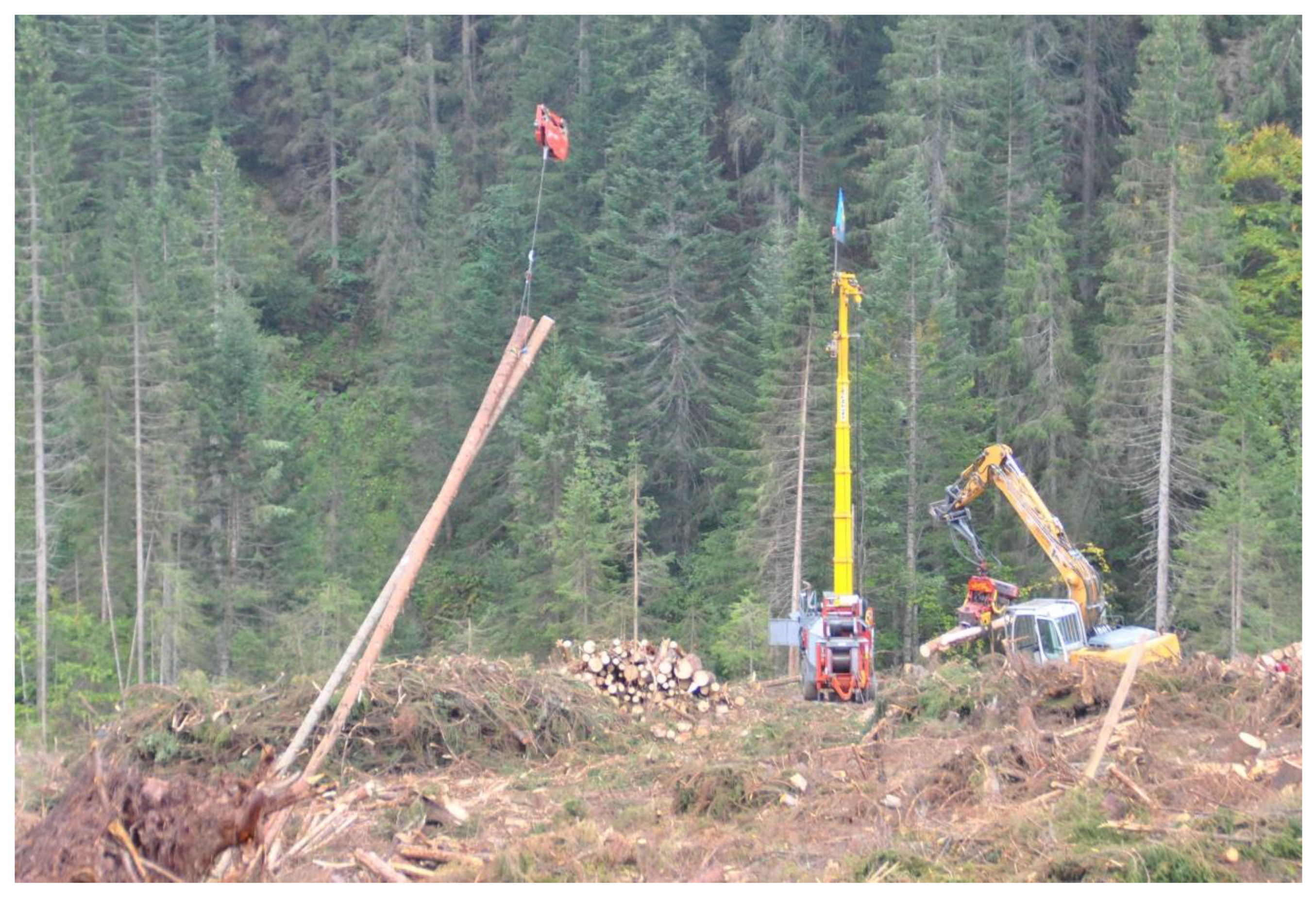
All study operators used modern Valentini tower yarders, except for the Lombard contractor who had a Konrad Woodliner (

Table 1. Description of the test operations.

#	Placename	Operator	Stand	Treatment	Yarder	Crew	Lines	Direction	Span	Handle	2-Stage	kW
1	Cuvio (VA)	Lombardy	Hardwood	Clearcut	Konrad	3	1	Downhill	400	L	Y	230
2	Tolmezzo (UD)	FVG 1	Spruce	Salvage	V850	3	1	Downhill	250	L	N	255
3	Arta terme (UD)	FVG 1	Spruce	Salvage	V850	3	2	Uphill	300	L	N	255
4	Cleulis (UD)	FVG2	Hardwood	Selection	V400	3	1	Uphill	200	P	Y	460
5	Enemonzo (UD)	FVG2	Hardwood	Selection	V400	3	1	Uphill	100	P + L	N	220
6	Socchieve (UD)	FVG2	Spruce	Salvage	V400	4	2	Uphill	200	P + L	Y	460
7	Cere (TN)	Trentino	Spruce	Salvage	V600	4	9	Various	300	P	Y	660
8	Meone (UD)	FVG2	Spruce	Salvage	V400	3	3	Uphill	250	P + L	Y	220
9	Rigolato (UD)	FVG2	Spruce	Salvage	V400	3–4	2	Uphill	310	L	N	180
10	Forni Avoltri (UD)	FVG 3	Spruce	Salvage	V600	4	4	Downhill	550	P	Y	630
11	Piani di Luzza (UD)	FVG 3	Spruce	Salvage	V600	4	4	Downhill	550	P	Y	630
12	Pierabech (UD)	FVG 3	Spruce	Salvage	V600	4	3	Downhill	600	P	Y	630

Notes: The code between parentheses in the column “Placename” represents the province code; All the V models under the “Yarder” column are Valentini tower yarders; “Span” is the direct distance between the tower tip and the end mast, without slope correction; 2-Stage = intermediate transportation from the yarder landing to a roadside log yard; Handle = the equipment stationed by the yarder for handling the incoming load: L = excavator-based loader; P = excavator-based processor. If a loader is also present (sites 5, 6 and 8), then the processor focuses on delimbing and crosscutting, the loader on stacking; kW = sum of the rated engine power of all equipment used in the operation (yarder, processor, excavator, truck etc.).

, Figure 1). Except for the latter, all set-ups used mechanical self-clamping carriages, among which Hochleitner’s Bergwald was the most popular (e.g., Bergwald 3000, 4000 and 5000). Typically, three workers manned the yarder and the excavator-based processor (or loader); a fourth team member was often employed when two-staging was necessary. All set-ups adopted a standing skyline configuration, and the loads were always pulled towards the tower, which could be set uphill or downhill. In the latter case, a haulback line was installed, except for the Konrad Woodliner that could drive directly on the skyline and did not need any external winches to pull it up or down. All operators were experienced professionals, who had been engaged with forest work for many years and had a deep understanding of the techniques and equipment they used. In most cases, the owner of the company or one of his relatives was directly engaged with the work being performed.

Nine out of twelve operations were salvage cuts of spruce-dominated softwood stands, which had become the prevalent treatment in the Italian Alps for at least four years after the catastrophic windstorm Vaia in October 2018 [19]. The remaining three operations concerned hardwood stands: two were selection cuts, while the third was a clearcut, conducted on a typical coppice forest (the Lombard case).

The observation unit was the individual operation (n = 12). Records did not contain sufficient detail to attribute fuel consumption and time use to any individual day or cable line. Typically, contractors would refuel when the tank was close to empty or when a good opportunity presented itself (delay etc.), which did not occur every day or exactly when a line was completed and the next one was to be installed. While more detail would have allowed building more accurate models, we traded accuracy for power, preferring a robust model based on a larger number of operations and workdays to a sophisticated one based on fewer operations and workdays.

Data analysis started with estimating the breakdown of fuel consumption and time use over the different tasks. The next step was the extraction of descriptive statistics for estimating general reference values that could be used for benchmarking. Differences between groups were tested with non-parametric statistics, which were most suitable to the non-normal, unbalanced small dataset gathered with the study. Regression analysis was used to determine the shape and significance of any associations between variables—typically fuel use vs. operational conditions. For all analyses the significance level was α < 5%.

Overall, the dataset represented 12 operations that covered 40 ha and produced 6090 m³ of timber. That task required 8500 man-hours and 28,900 L of diesel fuel. Thirty-three cable lines were installed, with a mean span of 370 m (tower tip to end mast). The data covered all time and fuel consumption required for turning trees in the forest into logs stacked at a roadside yard.

3. Results

The study sites represented the typical small lots normally harvested in the European Alps [20]. Mean tract surface was between 2 and 3 ha, for a harvest of about 500 m³ (

Table 2. Study sites: descriptive statistics.

		Mean	Median	SD	SE	Min	Max	IQR	SUM
Surface	ha	3.7	3.4	1.3	0.4	2	7	1	44
Removal	m3	507	328	531	153	200	2100	345	6084
Stocking	m3 ha−1	139	94	143	41	54	583	50	-
Yarder power	kW	127	128	50	14	75	175	94	-
Sum power	kW	402	357	195	56	180	660	405	-
Lines	n	2.8	2.0	2.3	0.6	1	9	2.5	33
Span	m	334	300	158	46	100	600	250	-
Crew	n	3.5	3.4	0.5	0.1	3	4	1	-
Worksite time	days	21	15	21	6	9	85	9	252

Notes: SD = Standard Deviation; SE = Standard Error; IQR = Interquartile Range; Yarder power = Rated power of the yarder engine; Sum power = Sum of the rated powers of all engines at work; Span = direct distance between the tip of the tower and that of the end mast, not corrected for slope; Total time = Days the operation was active on the selected site, incl. commuting (travel time), non-work time up to half a day (e.g., disturbance, delays) and work time.

). Removal intensity varied greatly (from 50 to 500 m³ ha⁻¹) depending on stand conditions and silvicultural treatment. On average, harvesting took from 2 to 3 weeks and required the set-up of 2 to 3 lines—that is, one line per week. The mean power for the yarder alone was 127 kW, but this figure is strongly driven by the prevalence of two yarder models of very different sizes: the Valentini V400 powered by a 75 kW tractor and the Valentini V600/1000 powered by a 175 kW independent engine. The whole operation consisted of a yarder (75 to 175 kW), an excavator-based loader or processor (60 to 100 kW) and a truck for two-staging (250–300 kW) where intermediate transportation was necessary—that is 8 cases out of 12. As a result, the total power invested in an operation may easily climb to 400 kW or more. That figure excluded the power of the chainsaws used for felling (all cases) and processing (wherever a processor was not available). However, the power of the average chainsaw was about 2 kW and even if 4 or 5 chainsaws would be present at each operation, their contribution to total power was negligible.

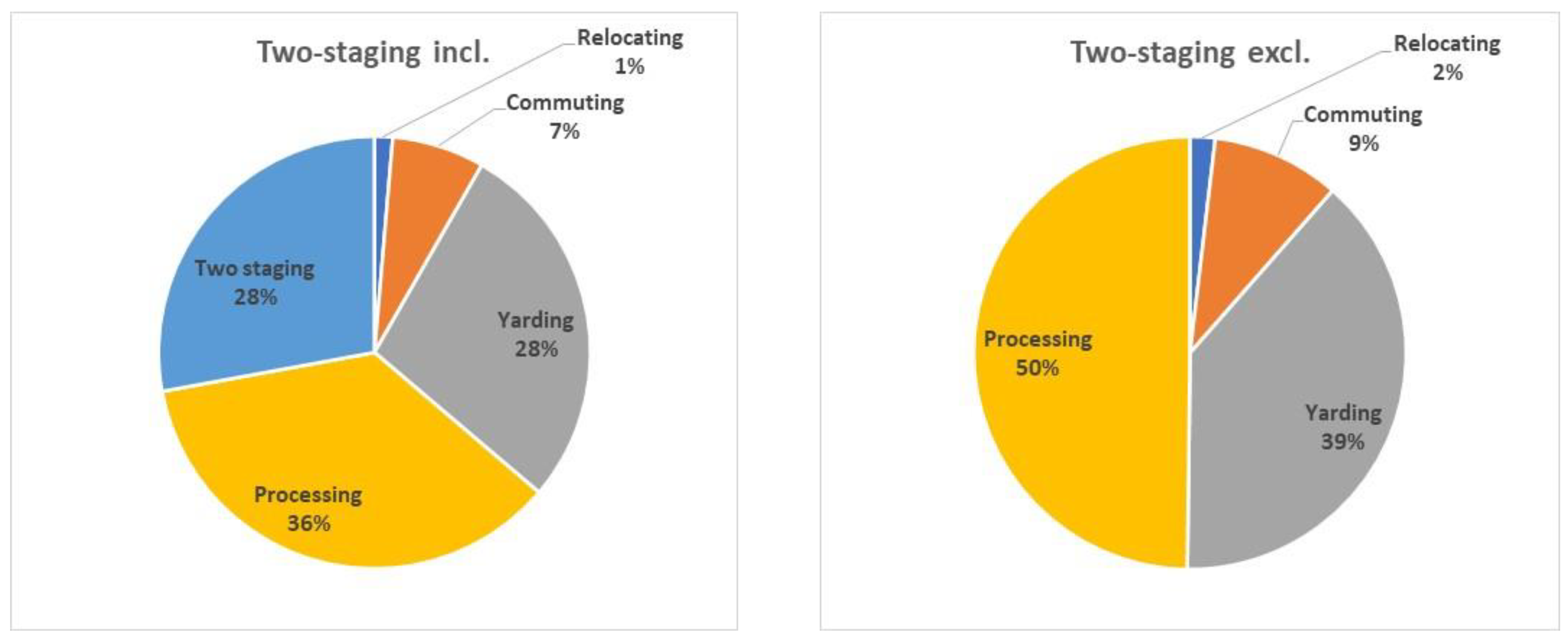
Overall, diesel fuel consumption was 12 to 50 times as large as the consumption of chainsaw fuel mix, and therefore most of the analysis focused on diesel fuel consumption. Taken as the grand total (sums of all operations), yarding accounted for a fraction of total diesel fuel consumption, assessed at one quarter of the total when two-staging was included, or 40% of the total if that was excluded (Figure 2). Taken as the mean of the breakdowns from each individual operation, that figure was 23% or 42%, depending on whether the operation required two staging or not. Interestingly, the contribution of the yarder to total diesel fuel consumption never exceeded 33%, when two staging was performed (

Table 3. Percent breakdown of total diesel fuel consumption among the main tasks (n = 12).

	Mean	Median	SD	SE	Min	Max	IQR
Including two-staging
Yarding	23.3	24.0	8.3	2.9	13.8	33.2	16.2
Yarding & Processing	58.3	62.2	17.3	6.1	26.5	77.6	23.4
Two-staging	33.7	32.3	16.0	5.7	13.9	60.6	25.2
Relocating	1.6	1.0	1.5	0.5	0.2	4.4	1.9
Commuting	6.5	6.3	2.7	1.0	3.1	11.6	3.3
Excluding two-staging
Yarding	41.8	42	16.2	8.1	23.4	59.8	26.1
Yarding & Processing	84.3	82.9	7.8	3.9	77.8	93.7	19.3
Two-staging	-	-	-	-	-	-	-
Relocating	4.9	3.5	4.3	2.1	1.6	11.1	5.4
Commuting	10.7	10.2	5.5	2.7	4.7	17.9	7.5

Notes: SD = Standard Deviation; SE = Standard Error; IQR = Interquartile Range.

). In all cases, the main fuel consumer was the excavator tasked with handling and processing the incoming loads. When performed, two-staging incurred about the same consumption as yarding alone, although that figure was extremely variable due to the large variations in two-staging distances, which ranged between 2 and 8 km. Unfortunately, that parameter was reported only in a minority of cases and therefore there were not enough data for regressing fuel consumption against two-staging distance. Equipment relocation between work sites contributed very little to overall fuel consumption, while the daily crew commutes had a variable impact, which may grow to represent over 10% when dealing with particularly remote sites (e.g., the operation in Cuvio, Lombardy).

In absolute terms, total fuel consumption averaged a whopping 5 L m⁻³ of diesel (

Table 4. Diesel fuel consumption (L m⁻³) by task: descriptive statistics.

	Mean	Median	SD	SE	Min	Max	IQR
Total	5.10	4.89	2.47	0.71	1.80	9.07	3.89
Yarding	1.32	1.27	0.56	0.16	0.62	2.14	1.02
Yarding & processing	3.15	2.71	1.40	0.41	1.40	6.37	1.85
Two-staging (8)	2.22	2.05	1.49	0.52	0.77	5.50	1.16
Relocating	0.10	0.10	0.08	0.02	0.01	0.25	0.11
Commuting	0.37	0.30	0.25	0.07	0.13	1.05	0.18
Yarding Uphill (6)	0.94	0.81	0.44	0.18	0.62	1.81	0.23
Yarding Downhill (5)	1.81	1.85	0.31	0.14	1.35	2.14	0.44

Notes: SD = Standard Deviation; SE = Standard Error; IQR = Interquartile Range; The Number in parentheses in the first column represents the number of observations (n). When no number is reported, then n = 12.

). Yarding alone incurred a fuel consumption between 0.8 and 1.8 L m⁻³ (interquartile range), with an average at 1.3 L m⁻³. When handling and processing were also included, the cumulated figure became over twice as large. Two-staging incurred a larger fuel consumption than yarding (≥2 L m⁻³). On top of that, the study operations consumed between 0.13 and 0.27 L m⁻³ of chainsaw fuel (interquartile range). In fact, chainsaw fuel consumption was significantly different depending on whether or not a processor was used; if it was used, mean chainsaw fuel consumption was 0.1 L m⁻³, if not fuel consumption expanded to 0.4 L m⁻³ (p = 0.0065, according to the Mann–Whitney test). Conversely, when trees were processed motor-manually and the excavator was only used for loading, the fuel consumption incurred by the excavator component averaged 0.74 L m⁻³, instead of 2.31 L m⁻³ as recorded for those cases where the excavator fleet was also tasked with mechanized processing (p = 0.0108, according to the Mann–Whitney test).

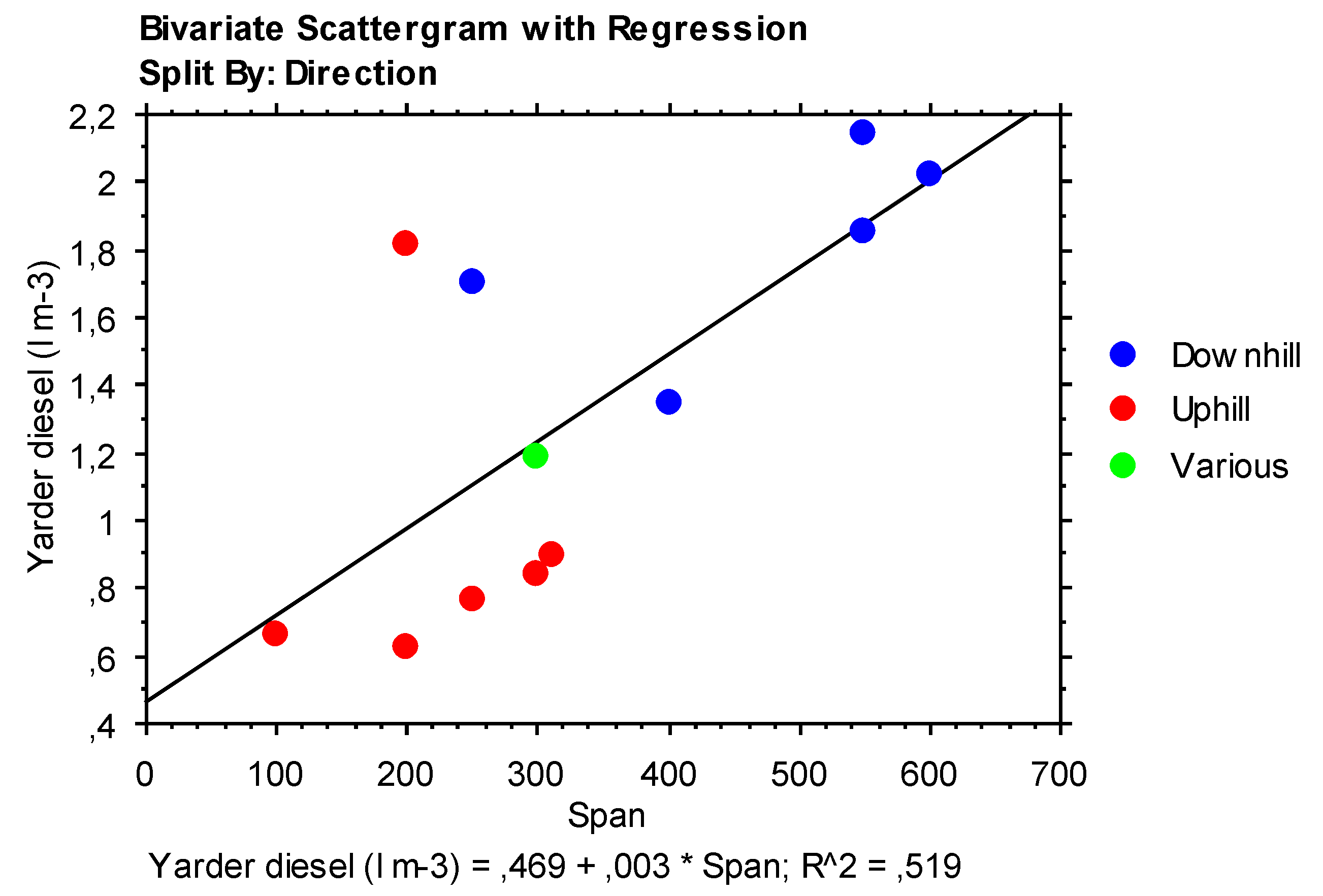
Data analysis showed a good correlation between yarder fuel consumption and line span (Figure 3). Consumption increased by 0.3 L m⁻³ for each additional 100 m of line span. Unfortunately, the data were badly unbalanced, since the longest spans were all powerful yarders (mean 175 kW) used for downhill extraction, while the shortest were much lighter yarders (mean 75 kW) used for uphill extraction. Therefore, it was impossible to determine how much of the additional fuel consumption incurred on the longer lines was due to the longer distance travelled, and how much to the larger engine power of the machines used for those jobs.

Production accounted for 40% to 70% of total time (man-hours; interquartile range), with a grand average at 57% (

Table 5. Percent breakdown of total time (man-hours) among the main tasks and time use per m³ and task (n = 12).

	Mean	Median	SD	SE	Min	Max	IQR
% over total time
Relocating	2.1	1.7	1.9	0.6	0.2	7.3	1.5
Setting up	22.0	13.3	21.0	6.1	3.1	60.6	30.9
Commuting	13.9	10.0	12.5	3.6	2.5	38.9	11.8
Production	55.6	58.2	17.4	5.0	27.8	84.4	28.3
Downtime	6.5	3.4	7.4	2.1	0.0	18.8	13.6
man-hours m−3
Relocating	0.032	0.020	0.040	0.012	0.002	0.153	0.010
Setting up	0.340	0.255	0.265	0.076	0.030	0.914	0.365
Commuting	0.208	0.143	0.361	0.104	0.025	1.344	0.119
Production	0.848	0.786	0.475	0.137	0.395	1.980	0.686
Downtime	0.100	0.052	0.125	0.036	0.000	0.330	0.192

Notes: SD = Standard Deviation; SE = Standard Error; IQR = Interquartile Range.

). Large downtime events represented between 3 and 6% of total time (man-hours): however, that figure only accounted for major time-loss occurrences, when all work came to a halt due to bad weather, serious breakdown or massive interference (e.g. rescuing another operation). All the recurrent downtime that characterized the operation of a single piece of equipment was not recorded separately and was lumped with production. Therefore, production time also included a whole range of delay events, with variable individual durations.

Overall, time consumption amounted to 1.5 man-hours m⁻³. That included all tasks in the list, namely: relocation, setting up, commuting, production and large downtime (

Table 6. Time consumption (man-hour m⁻³): descriptive statistics.

Time	Processor	n	Mean	Median	SD	SE	Min	Max	IQR
All	All together	12	1.53	1.24	0.74	0.21	0.95	3.54	0.78
All	No	4	1.97	1.67	1.13	0.56	1.02	3.54	1.66
All	Yes	8	1.31	1.21	0.38	0.38	0.95	2.09	0.50
Production	All together	12	0.85	0.79	0.47	0.14	0.39	1.98	0.69
Production	No	4	1.16	1.06	0.63	0.31	0.54	1.98	0.94
Production	Yes	8	0.69	0.62	0.32	0.11	0.39	1.26	0.47

Notes: n = number of observations; SD = Standard Deviation; SE = Standard Error; IQR = Interquartile Range; All = time consumption for all tasks; Production = time consumption relative to production only (felling, yarding and processing), and excluding: relocation, set up and dismantle, commuting and major downtime; Processor = whether the operation uses a mechanized processor or just a loader.

). If the analysis was restricted to production only, then time consumption would amount to 0.85 man-hour m⁻³. In fact, there was a large difference between the productivity of the operations equipped with a processor and those with a loader, only—the former using 70% less man-hours than the latter. With p = 0.08, the Mann–Whitney test indicated that such difference was not significant at the 5% level, but it was still highly suggestive. In contrast, two-staging had a much smaller effect: overall time consumption averaged 1.6 man-hours m⁻³ when two-staging was necessary and 1.3 man-hours m⁻³ when it was not. As expected, time use was higher when two-staging was applied, but the difference was relatively small (23%) and was not statistically significant (p = 0.50 according to the Mann–Whitney test). Of course, lack of statistical significance did not prove that two-staging had no impact on overall time use, but simply that this study was not designed to gauge the effect of two-staging on time consumption and therefore the results of the comparison for two-staging may have been confounded by uncontrolled background noise.

Set-up and dismantling were the second largest consumers and occupied 22% of the total time invested in the operation. Mean set-up and dismantling time was 12 h (43 man-hours) per line (

Table 7. Set-up and dismantling: main descriptive statistics (n = 12).

		Mean	Median	SD	SE	Min	Max	IQR
	Uphill & Downhill Yarding (33 lines)
Span	m	337	300	166	50	100	600	300
Time	h line−1	12	9	8	3	2	26	14
Time	man-hour line−1	43	32	35	11	8	104	58
Time	man-hour m−3	0.30	0.26	0.26	0.08	0.10	0.91	0.36
Time	% man-hour	22	9	22	7	3	61	34
	Downhill Yarding only (13 lines)
Span	m	470	550	144	64	250	600	200
Time	h line−1	18	22	9	4	5	26	14
Time	man-hour line−1	68	88	40	18	15	104	67
Time	man-hour m−3	0.45	0.51	0.33	0.15	0.75	0.91	0.50
Time	% man-hour	34	43	27	12	5	61	52
	Uphill Yarding only (11 lines)
Span	m	227	225	78	32	100	310	100
Time	h line−1	7	7	3	1	2	11	5
Time	man-hour line−1	22	21	10	4	8	36	16
Time	man-hour m−3	0.18	0. 13	0.16	0.06	0.10	0.37	0.32
Time	% man-hour	12	8	10	4	3	30	13

Notes: SD = Standard Deviation; SE = Standard Error; IQR = Interquartile Range.

). In fact, there was a marked difference between uphill and downhill yarding set-ups: the latter spanned longer distances and took more time and people to install and dismantle (18 h vs. 7 h; 4 people vs. 3 people). The longer set up and dismantling time was likely related to such challenges as the need to drag the cables uphill and to install an additional line–the haulback line–when rigging the yarder for downhill extraction. Furthermore, few of the lines rigged for uphill yarding required intermediate supports, while the contrary was true for those lines that had been designed for downhill yarding. With one exception, the latter always required at least one intermediate support, occasionally two or even three. However, the systematic span length difference made it impossible to correctly attribute the additional set-up time to either span length or system configuration. Therefore, all one could say was that it took more time and work to install longer lines designed for downhill extraction, than it did to setup shorter lines designed for uphill extraction.

Contrary to set-up and dismantling, equipment relocation between worksites seemed to have a negligible impact on time consumption, which was consistent with a modest fuel expenditure. Equipment relocation often took 2 or 3 trips, conducted over relatively short distances (

Table 8. Relocation: main descriptive statistics (n = 12).

		Mean	Median	SD	SE	Min	Max	IQR
Trips	n°	2.7	2.0	1.1	0.3	2.0	5.0	1.5
One-way distance	Km	13.6	12.0	9.5	2.8	3.0	30.0	18.5
Total distance	Km	65.2	60.0	39.9	11.5	16.0	128.0	69.0
Time use	h	7.7	6.5	3.5	1.0	4.0	13.0	6.0
Time use	man-hour	9.5	6.5	8.1	2.3	4.0	33.0	7.0
Time use	% man-hour	2.1	1.7	1.9	0.6	0.2	7.3	1.5
Diesel consumption	% Total l	2.7	1.7	3.0	0.9	0.2	11.1	3.0

Notes: SD = Standard Deviation; SE = Standard Error; IQR = Interquartile Range.

). The maximum relocation distance recorded in this study was 30 km, which may point at a good operational planning and more in general at the presence of a local business model, where resident companies focus on sales that are available in the immediate vicinity, so as to cut down on relocation and commuting time and cost.

Nevertheless, commuting had a visible impact on time use. It was the third largest contributor after production and set-up. Clearly, its repetitive nature led to each commute to add up until the total contribution was large enough to stick out. Commuting distance was indeed relatively short, ranging most often from 10 to 15 km, but the roads travelled were generally slow and the shortest commuting time was half an hour, one way. Shorter commutes invited crews to go back home for lunch, which doubled the number of commutes and inflated commuting time. All crews commuted together in a single vehicle: a crew-cab pick-up truck or a minivan. So, both the vehicles and the routines (joint rides) were fuel-efficient, which helped minimize fuel consumption. Yet, fuel consumption was relevant because the roads were steep, winding and often low standard for a large part, which imposed travelling on a low gear, a high rpm and often in the 4WD mode. Overall, results point at the notable impact of commuting time, which should not be underestimated.

4. Discussion

As a start, it is most appropriate to discuss the main limitations of this study; namely, the local bias towards one particular area in the European Alps, the relatively small number of observations and the reliance on company records.

Concerning local bias, it is a fact that 10 out of 12 operations were located in one region of Northeastern Italy (Carnia). For that reason, one may wonder about the capacity of such a localized sample to represent yarder operations across the Alps, or even across Italy. That is a sensible objection: caution should be taken when extending the results of this study outside Northeastern Italy. However, the technology represented in our data is common to most Alpine loggers. Light and medium-sized tower yarders are widespread in the whole region, and the machine types represented in the sample are bestsellers that are very popular across the Alps. The same can be said for operational layout, with the typical association of a tower yarder and an excavator-based processor or loader. That is indeed the Alpine standard for modern cable logging operations, which come in many variations. Furthermore, lot size was comparable with the figures reported in recent literature for France, Italy, Germany, Slovenia and Switzerland [20]. Similarly, forest types, stand characteristics, silviculture and terrain are relatively homogenous across the Alpine continuum [21]. Finally, the area of interest—Carnia—is located in the so-called three-borders mountains, where Italy meets with Austria and Slovenia and national traditions, know-how and economies meet and eventually mix. Paradoxically, narrow localization in one region may have made this study representative of a cross-border area that is much larger than a better Italian spread would have allowed. The main thing one could question is the prevalence of salvage operation in our sample, which are not representative of ordinary forest management. In fact, the frequency and size of forest disturbance events have dramatically increased in the Alps [22] and generally in Europe [23], and they are likely to become a main driver of forest management in the near future.

The small number of observations is another limitation. Obviously, we would have liked to get a larger sample, and ConAIBo did try hard to recruit more of their members into the initiative, even offering financial incentives. However, the enormous surge in logging service demand consequent to the 2018 windstorm had loggers placing all their energies and attention onto production, so that few were willing to get even a minimal distraction in the way of an exhausting (but rewarding) job. Those who joined the study often did so due to the strong personal ties with their representative at the Regional Association, and in that regard the coordinator for Friuli Venezia Giulia was the most successful. In fact, the study examined a few more candidates than eventually accepted, but it included only those who had a proven professional record and were equipped with modern and typical machinery—for the very purpose of obtaining a representative sample that could be used to reflect work conditions in the larger Alpine region. Our 5 contractors represent a much smaller sample than the 21 sampled by Kuhmaier et al. [10] or the 28 recruited by Oyer and Visser [11]. Yet, they were taken to represent a relatively uniform technology level and operational mode, and the sample still included over 30 corridors and 250 worker days, which is not a small amount in absolute terms. Moreover, the data were used for extracting general reference values, not accurate models, and for that use they were likely adequate.

Delegating data collection to company compilers rather than performing direct measurements by professional researchers may have represented a further limitation, due to the variable accuracy of such a data collection method. In particular, company records may be flawed by omission, approximation and transcription errors derived from rushed or incomplete compilation. Furthermore, those records may present wrong allocation of time or fuel records, or the lumping of different items into a single cumulated figure. Some of those limitations were overcome by aggregating minor items into larger categories, which were most likely recorded in the same way. That made the dataset robust against inaccurate recording. As a matter of fact, the overall consistency of the dataset shows that contractor records were accurate enough for the purpose of this study. Flagrant errors would have been exposed by the large variations in the data scatter and/or the presence of extravagant outliers, neither of which was apparent at a first examination of the data cloud.

In fact, comparison with the fuel consumption data reported in other studies seems to corroborate our results (Table 9). Our numbers are definitely within the ballpark: specific yarder and processor figures offer a reasonably close match to those reported for other yarders, which supports the notion of a workable accuracy. In that regard, the main additional contribution offered by our study is that of providing a detailed breakdown of fuel consumption by task, and/or including fuel consumption items that were not covered in the other studies, such as commuting, two-staging and relocation. Incidentally, the only study that reports figures for relocation, quantifies that expenditure at 0.13 l m⁻³, which is very close to our 0.10 L m⁻³ [8]. Similarly, our chainsaw fuel consumption figures for motor-manual felling and processing (0.4 L m⁻³) reflect quite well those reported by Argnani (0.37 L m⁻³) and Popovici (0.43 L m⁻³) for the same type of work [24,25].

All trends were plausible: they matched predictions and reflected anecdotal evidence. It was just too bad that data unbalance made it impossible to check for any yarder configuration effects, that is: if the braking power applied to the haulback line in the downhill configuration would result in a larger or smaller energy drain than caused by the need to fight gravity in the uphill configuration. Anecdotal evidence points at a significant energy expenditure incurred when pulling a load downhill against the resistance offered by the haulback line, which adds to the workload imposed by moving a very long cable loop. For that reason, many loggers estimate that fuel consumption could be higher for downhill yarding compared with uphill yarding, which may sound counterintuitive at first. As they stood, our results could not offer much help in that sense: they did identify a trend but could not distribute it clearly among several independent variables. In fact, the larger fuel consumption recorded for longer spans might simply be the result of productivity declining with extraction distance, which is a logical, well know phenomenon, generally modelled through linear functions [26]. When yarding distance increases, the yarder engine is under load for longer in order to extract the same load, which results in a higher fuel consumption per m³. Since the processor (or loader) depends on the yarder, its productivity will also decline, but that machine will idle when waiting, so fuel use per product unit will not increase—which is what the data showed, through the inconclusive regressing of processor fuel consumption vs. line span (R² = 0.0022).

Table 9. Comparison with the results from other fuel consumption studies.

Country	Forest	System	L m−3	Source	Notes
Sweden	Boreal	CTL	1.5	[1]
Finland	Boreal	CTL	1.2	[1]
Canada	Boreal	CTL	2.0	[27]
Finland	Boreal	CTL	1.2 to 2.8	[8]	Highest thin, lowest clearcut
Australia	Hardwood plantation	CTL	1.4	[27]
Ireland	Softwood plantation	CTL	2.4	[2]
South Africa	Softwood plantation	CTL	1.2	[28]
Austria	Temperate softwood	CTL	1.6	[27]
Croatia	Temperate	Skidder only	1.1 to 1.7	[29]
Canada	Boreal	WTH	2.7	[27]
Australia	Hardwood plantation	WTH	2.6	[27]
New Zealand	Softwood plantation	WTH	3.0	[11]
USA	Softwood plantation	WTH	2.2	[30]
New Zealand	Softwood plantation	Yarding	2.3 to 3.4	[11]
New Zealand	Softwood plantation	Yarding	2.3 to 2.8	[31]
New Zealand	Softwood plantation	Yarding	2.8 to 3.0	[32]
New Zealand	Softwood plantation	Yarding	2.7 to 3.4	[33]
Austria	Temperate softwood	Yarding	2.2	[27]	Yarder and processor
Austria	Temperate softwood	Yarding	0.9 to 1.3	[12]	Yarder and processor
Italy	Temperate softwood	Yarding	3.1	This study	Yarder and processor
Italy	Temperate softwood	Yarding	1.3	This study	Yarder only

Table 9. Comparison with the results from other fuel consumption studies.

Country	Forest	System	L m−3	Source	Notes
Sweden	Boreal	CTL	1.5	[1]
Finland	Boreal	CTL	1.2	[1]
Canada	Boreal	CTL	2.0	[27]
Finland	Boreal	CTL	1.2 to 2.8	[8]	Highest thin, lowest clearcut
Australia	Hardwood plantation	CTL	1.4	[27]
Ireland	Softwood plantation	CTL	2.4	[2]
South Africa	Softwood plantation	CTL	1.2	[28]
Austria	Temperate softwood	CTL	1.6	[27]
Croatia	Temperate	Skidder only	1.1 to 1.7	[29]
Canada	Boreal	WTH	2.7	[27]
Australia	Hardwood plantation	WTH	2.6	[27]
New Zealand	Softwood plantation	WTH	3.0	[11]
USA	Softwood plantation	WTH	2.2	[30]
New Zealand	Softwood plantation	Yarding	2.3 to 3.4	[11]
New Zealand	Softwood plantation	Yarding	2.3 to 2.8	[31]
New Zealand	Softwood plantation	Yarding	2.8 to 3.0	[32]
New Zealand	Softwood plantation	Yarding	2.7 to 3.4	[33]
Austria	Temperate softwood	Yarding	2.2	[27]	Yarder and processor
Austria	Temperate softwood	Yarding	0.9 to 1.3	[12]	Yarder and processor
Italy	Temperate softwood	Yarding	3.1	This study	Yarder and processor
Italy	Temperate softwood	Yarding	1.3	This study	Yarder only

The study makes it clear that the yarder alone accounts for less than half of the total fuel consumption. When necessary, two-staging incurs an additional fuel consumption that is about as large. In fact, the main fuel user is the processor. It is worth noticing that all processors used in this study are excavator-based machines, notoriously flawed by high fuel consumption, compared with dedicated CTL harvesters and processors [34]. That may also explain why our fuel consumption figures are much higher than those reported for Austrian yarding operations [12,27]: the Austrian studies concern integrated yarder-processors, where the processor is part of the yarding unit and is run by the same engine as the tower winches, through an optimized interface. In contrast, most excavator-based processors are obtained through the crude matching of a series-production earth-moving machine with a heavy harvester head. Such contraptions rarely benefit from the same sophisticated power management as available on purpose-built processors, and even when optimized adaptation kits are installed, the fuel saving benefits are relatively small [35]. In fact, yarder contractors tend to favor excavator-based machines because of their lower price, stronger boom and all-round rotation capacity [36]. The results of the study indicate that an efficient strategy to curb on fuel consumption should include technology development, machine selection and operational planning. Of course, one should try and recover much of the energy dissipated by the yarder when fighting against gravity, possibly through electric or hybrid-electric solutions [13]. Along with that, one should try and develop better power management software for the associated excavator-based processor, or—better yet—integrate the processor with the yarder and manage both machines through an electric-hybrid power pack fit for energy recuperation. Finally, one should improve the forest road standard to reduce the need for two-staging, which uses as much fuel as yarding itself.

The latter measure will also have an impact on commuting efficiency, which may not be negligible, given that commuting represents a meaningful source of fuel and time consumption. Better roads will make for faster and more efficient commutes, further reducing fuel consumption and time use. In fact, commuting is a societal problem that goes far beyond the narrow field of forestry and impacts all occupations [37,38]. The mean commute time recorded in this study does not deviate much from the European averages for rural workers [39] which—incidentally—have not changed much since the 1960s [40]. In this case, the main concern is that harvesting crews tend to commute in the early morning, when the risk for crashes is highest [41].

The results from the time use analysis further corroborate the general validity of this study. The 0.69 man-hours m⁻³ reported here for mechanized work closely match the 0.80 man-hour m⁻³ reported in an earlier mechanized cable yarding study, considering that the latter figure included set-up and dismantling, and the former did not [42]. If we add the mean set-up and dismantling time recorded in this study (0.30 man-hour m⁻³), then our figure increases to 0.99 man-hour m⁻³, which is still within the ballpark, although slightly higher. In fact, the extra time consumption could be easily explained by the challenging work conditions faced in the many windblown stands included in our sample. The inherent difficulty of salvage operations is the likely reason why set up and dismantle time was higher here than in the seminal study by Stampfer et al. [43]: that study reports an average set up and dismantle time of 9 h or 27 man-hours, which is respectively 25% and 40% shorter than in this study. The Austrian figures were obtained under the same mean span of 300 m, so distance was not a factor; however, the challenge of moving through a windblown stand for installing the yarder may explain the difference. Furthermore, it is possible that part (or most) of the felling was performed during set up, which is common practice among some crews. However, the forms did not report that detail, so it is impossible to know exactly what the cause was for the longer set up and dismantle time, and if part of that time should rather be transferred to production. When it comes to set up times and line span, a final remark can be made on harvest density—that is the amount of wood collected for each meter of line. In this study, the mean wood density was 0.8 m³ m⁻¹, which proved an exact match for the figures reported earlier on by Cavalli et al. [44] for northeastern Italy and landed quite close to the figures reported for the Bavarian State Administration on the other side of the Alps (1 m³ m⁻¹) [45], which are considered the optimum for effective operation [46]. That is one more witness to the professional competence of the studied teams and to a credible data set.

5. Conclusions

To our knowledge, this is so far the only scientific study offering real-life data about the fuel consumption and time use of European yarding operations, for all their activities. The other studies yet available focus on the yarder component only—not the whole operation–or reflect other conditions than those encountered in Europe. Moreover, our data represent typical small-scale operations conducted by private companies, which are prevalent in the Alps. The study makes it clear that supportive tasks (e.g., commuting, set up and dismantle) that are generally neglected by other studies do incur meaningful time and/or fuel consumption and should be included in all rationalization efforts. Yarding proper only accounts for less than half of the total fuel consumption; in fact, the main fuel user is the excavator-based processor. Furthermore, large fuel use is incurred by intermediate transportation between the yarder pad and a proper roadside landing, when the former is not accessible to conventional road rigs—which is a frequent occurrence in alpine operations. Therefore, significant fuel savings might be accrued by improving the forest road network, if that incurred acceptable financial and environmental cost.