Dynamic Changes of Plantations and Natural Forests in the Middle Reaches of the Yangtze River and Their Relationship with Climatic Factors

Abstract

Based on Landsat TM/ETM/OLI images and MODIS NDVI time series remote sensing data from 1999 to 2015, the changes of land use/cover types (including natural forests and plantations) through NDVI trends and their relationship with meteorological factors in the middle reaches of the Yangtze River (MRYR) were analyzed by supervised classification, coefficient of variation, trend analysis, rescaled range analysis, and partial correlation analysis. The results showed that, in the past 17 years, the main landscape type in the MRYR is forestland (accounting for more than 50%), and the built-up land and plantations area increased by four fifths and one fifth, respectively. The area of natural forests had been reduced by one fifth. Additionally, NDVI showed an upward trend (0.37%), especially in natural forests (0.57%). Two thirds of the natural forests had NDVI values greater than 0.80, and 89.21% of them were significantly improved. The area with an uncertain future development trend of all vegetation was more than half of the area. At the same time, partial correlation analysis with climate factors showed that relative humidity had an inhibitory effect on vegetation growth (p < 0.05). Climate factors had a certain lag effect on the growth of natural forests and plantations. Generally speaking, sunshine duration had a positive effect on forests growth, while relative humidity had a negative effect. The results showed that if the forest land was studied as a whole, many of the problems of natural forests and plantations would be ignored. The continuous decrease of natural forests and possible further degradation in the future are worthy of attention. The results could provide a reference for forest ecological protection in other areas.

1. Introduction

Vegetation, as the core component of the terrestrial ecosystem, is the link between the atmosphere, soil, water, and other natural factors in the ecosystem. It plays an important role in soil and water conservation, climate regulation, and the stability of the ecological environment [1,2,3]. Vegetation change is easily affected by climate. Under the trend of global warming, it has important theoretical value and there are application prospects to study the vegetation distribution, growth status, and vegetation structure response to meteorological factors [4,5,6]. With the continuous development and maturity of remote sensing technology, vegetation remote sensing data has become a key data source for monitoring global and regional land cover change. The Normalized Difference vegetation index (NDVI) is the most commonly used indicator to characterize vegetation growth status and coverage, and it is widely used in the study of vegetation change and its driving factors [7,8,9].

The middle reaches of the Yangtze River (MRYR), including Hunan Province, Hubei Province, and Jiangxi Province, is the core area of the development of the Yangtze River economic belt, and also the key area of China’s “two screens and three belts” ecological security strategy. The region has important ecological functions such as water conservation and regulation, biodiversity protection, and basin ecological security. It plays an important role in the ecological security and ecosystem stability of China and even East Asia [10]. In recent years, due to the impact of climate change and human activities, the ecological environment of the region has been deteriorating, and the problem of ecosystem degradation is becoming increasingly prominent, which poses a serious threat to the water resource conditions, ecological security, and sustainable development of the social economy of the region and the whole Yangtze River Basin [11]. The change of vegetation ecosystem in the MRYR has not only attracted the attention of scholars at home and abroad, but has also been highly valued by the Chinese government [12].

In 2005, China plans to invest USD 1134.94 million to start 22 ecological protection projects, including returning grazing land to grassland, returning farmland to forests, and harnessing ecologically deteriorated land [13,14]. According to the results of the Eighth National Forest Inventory (2009–2013), China’s plantation area was 69.33 million ha, accounting for 36% of the forests area and for 17% of the national forests volume, and the plantation scale ranks first in the world [15,16]. The results of the Ninth National Forest Inventory (2014–2019) showed that the area of plantations (5.02 million ha) is larger than that of natural forests (5 million ha) in some provinces of the MRYR, but the volume was lower than that of natural forests (180.65 million m³ of plantations; 226.51 million m³ of natural forests) [17]. The community structure of plantations and natural forests was usually different, the composition of plantations was relatively single, and the ecological stability was fragile [18,19]. Many scholars have studied the differences of community structure and soil components of plantations at the stand scale, but there are few studies on the differences of landscape patterns and vegetation dynamics between plantations and natural forests [20,21,22]. Analyzing the dynamic changes of land use types and vegetation in the MRYR before and after the implementation of ecological projects, especially the differences of dynamic changes of vegetation between plantations and natural forests and evaluating and measuring the effect of ecological protection projects, could provide an important scientific basis for evaluating the ecological benefits of ecological projects and guiding the construction and layout of plantations projects.

Vegetation is very sensitive to climate change [23,24]. At present, scholars at home and abroad have carried out a significant amount of research on the impact of climate on vegetation change [25]. In previous studies, many researchers used correlation analysis, multiple linear regression, and other methods to reveal that precipitation and temperature were the main meteorological factors affecting vegetation change [3,26,27,28]. However, there were also relevant studies concluding that vegetation changes were not only related to precipitation and temperature, but also that other meteorological factors (such as sunshine hours and relative humidity) had different effects on vegetation change [29,30,31]. The slow process of vegetation growth determined that the responses of vegetation change to meteorological factors had a certain lag and cumulative effect [32]. The responses of vegetation to meteorological factors had spatial heterogeneity in different spatial scales and vegetation types [26,33,34,35]. The results showed that NDVI was increasing year by year. The Yangtze River Basin is rich in water and the heat condition is the limiting factor affecting vegetation growth [36]. Yi et al. studied the responses of vegetation to climate change in the MRYR and pointed out that vegetation had an obvious time lag to climate change. But at present, there have been few studies comparing the dynamic characteristics of NDVI and its responses to climate change between plantations and natural forests in the same region [37]. Understanding and revealing the internal relationship between different vegetation types and meteorological factors is of great significance for regional ecological protection and management [38].

Remote sensing data can be used to identify vegetation types, mainly using the differences of spectrum, texture, and other characteristics of different vegetation types. Texture can be understood as the spatial change and repetition of image gray, or the repeated local patterns (texture units) and their arrangement rules in the image. Haralick first proposed the gray level co-occurrence moment (GLCM) [39]. This method uses a spatial co-occurrence matrix to calculate the relationship between pixel values and uses these values to calculate the second-order statistical properties of the matrix. GLCM is a widely used texture statistical analysis method and texture measurement technology. In the MRYR in China, plantations usually have single biodiversity and exist in patches of one or two plant species, such as Masson Pine, Chinese fir, and Chinese thuja. Compared with natural forests, this kind of plantation has more regular texture characteristics. Similarly, the plantations in eastern Thailand also have special texture features, which makes it possible to use texture features to identify their distribution law [40]. In southern Africa, the texture features of vegetation are used to identify invasive species [41]. At present, the GLCM has been widely used in image retrieval and classification, and it has greatly improved the accuracy of image retrieval and classification [42].

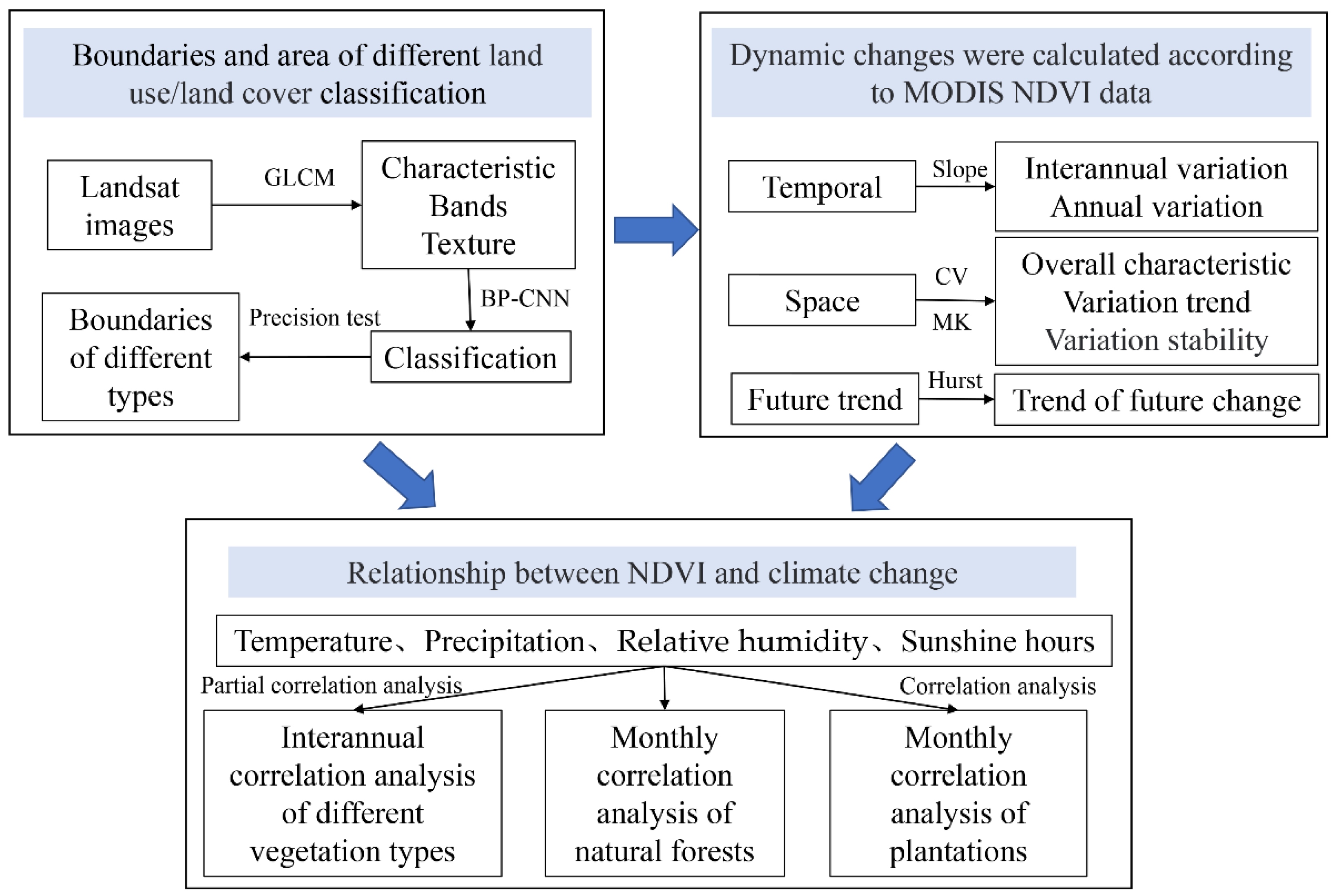
In this study, Hubei Province, Hunan Province, and Jiangxi Province in the MRYR are taken as the research objects, and four Landsat TM/ETM/OLI remote sensing images in 1999, 2005, 2010, and 2015 are taken as the basic data source. Based on the GLCM and spectral features, the neural network supervised classification method was used to classify the land use types in the study area, and the forest land was further divided into artificial forest and natural forest for analysis. Our specific objectives are: (1) to analyze the temporal and spatial change characteristics of land use (including natural forest and plantation) in the study area from 1999 to 2015; (2) to investigate the characteristics and evolution trends of NDVI of different vegetation types in the MRYR; (3) to analyze the relationship between meteorological factors and NDVI at interannual and monthly scales. This study reveals the dynamic changes of land use/cover types and the response mechanism of vegetation to climate change in the MRYR, especially natural forests and plantations. Our research can provide a scientific reference for regional ecological environment construction and protection measures.

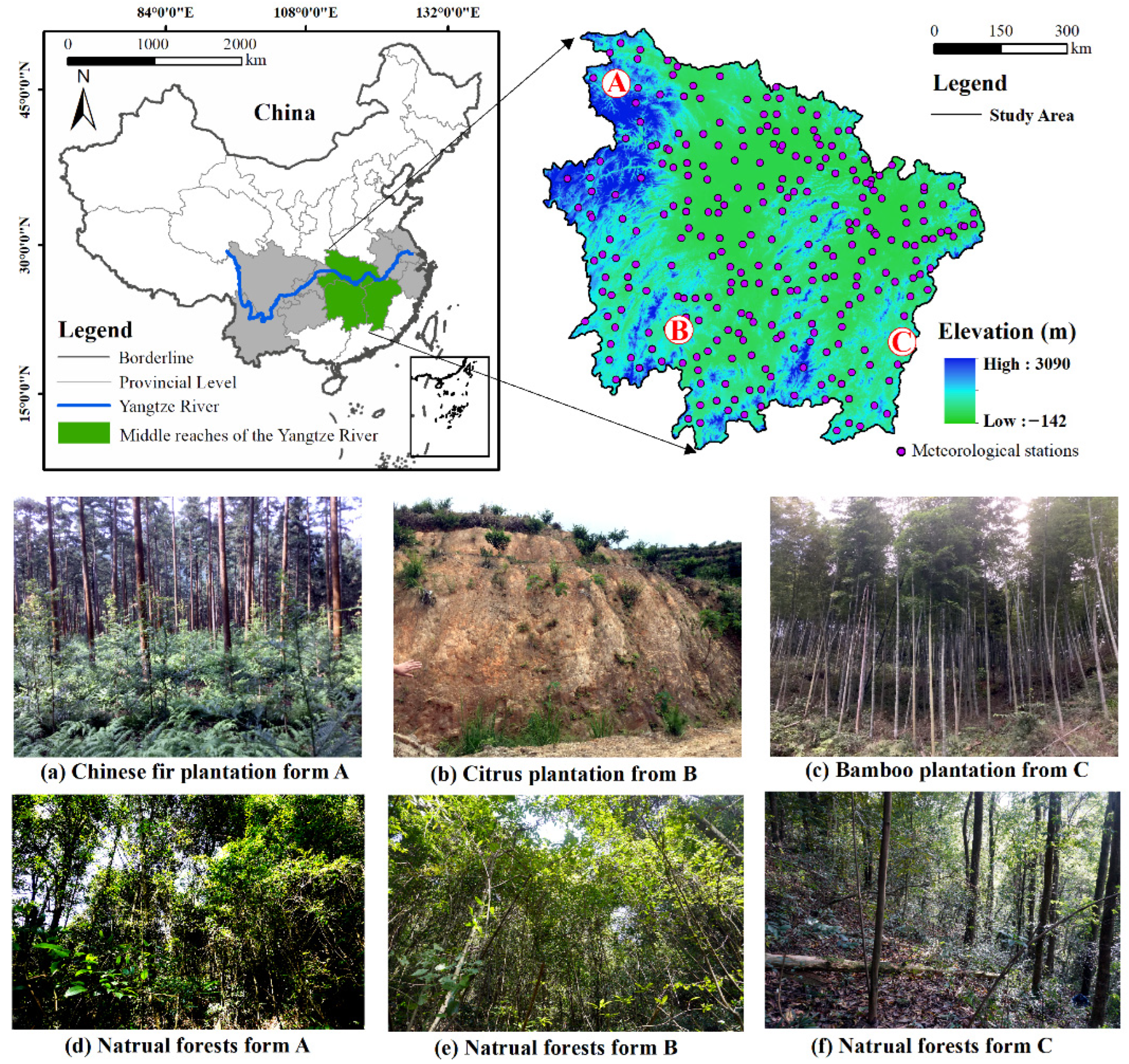
2. Study Area

The MRYR includes Hubei Province, Jiangxi Province, and Hunan Province (24°25’ N–33°16′ N, 108°24′ E–118°23′ E), with a total area of 564,600 km² (Figure 1). There are flat plains, hills, and steep mountains in this area. In the long process of development, traditional agriculture, forestry, and fishery production and splendid cultural and artistic landscape have formed in this area, which has had an important impact on the local land use [43,44]. The area over the general terrain is mountainous. The terrain is high in the west and low in the east, and the average altitude is approximately 1497 m [36]. The MRYR is rich in forest resources. In 2018, there were 174.38 million permanent residents in the MRYR, accounting for 12.7% of Chinese total population. The annual gross regional product (GDP) reached USD 1479.50 billion, accounting for 10.9% of the Chinese total GDP [45].

The plantations in the study area have a simple diversity of species, often consisting of one or two species of trees, such as Chinese fir, Masson pine, and Chinese thuja, etc. (Figure 1a–c). The natural forest is rich in plant diversity, mainly composed of Cinnamomum, Ligustrum, and Koelreuteria, etc. (Figure 1d–f). The vegetation under these plantations is relatively uniform and has regular texture characteristics, which are different from natural forests.

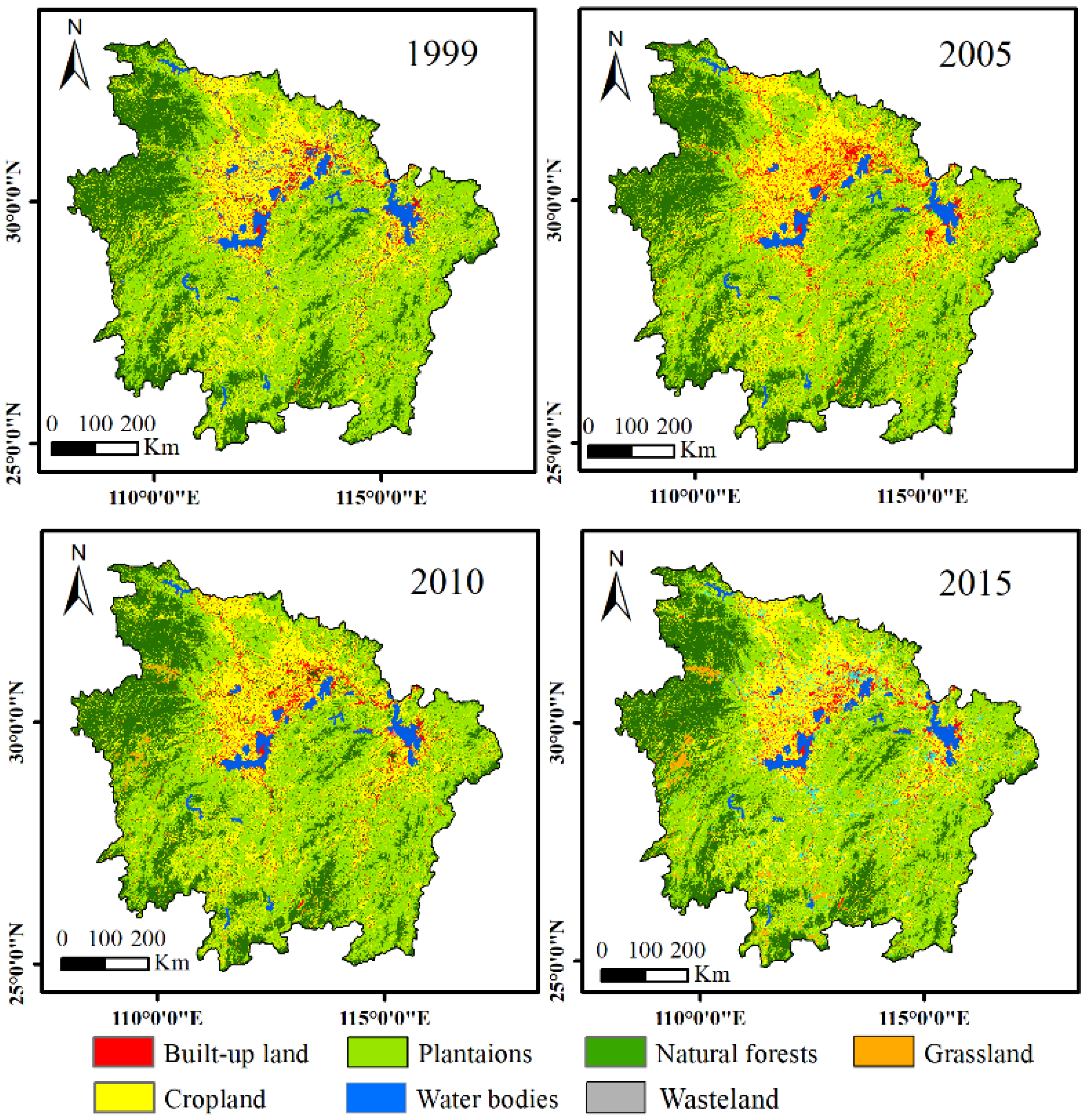
3. Data and Methods

3.1. Data Source and Preprocessing

The Landsat TM/ETM/OLI data used in this study are from the China geospatial data cloud (http://www.gscloud.cn/, accessed on 15 April 2021) (

Table A1. Remote sensing data used in the study.

Sensor	Dates	Cloud Amount	Path/Row	Resolution (m)
Landsat 4-5 TM	1999	≤10%	121-127/37-43	30/120 × (30)
Landsat 4-5 TM	2005	≤10%	121-127/37-43	30/120 × (30)
Landsat 4-5 TM	2010	≤10%	121-127/37-43	30/120 × (30)
Landsat 8 OLI	2015	≤10%	121-127/37-43	30/100 × (30)

). The NDVI data product is MODIS NDVI data from 1999 to 2015, which is derived from NASA’s MOD13A2 (https://wist.echo.nasa.gov/ap, accessed on 15 April 2021). Considering the integrity and quality of the data, we choose to use a spatial resolution of 1 km × 1 km, and the time resolution is 16 d. The acquired data are preprocessed by ENVI 5.3 and ArcGIS 9.3, including atmospheric correction, radiation correction, clipping, and stitching. The monthly data (of relative humidity, sunshine hours, air temperature, precipitation) were obtained from 272 benchmark meteorological stations near the study area for the period from 1999 to 2015 (http://data.cma.cn, accessed on 15 April 2021).

3.2. Research Method

3.2.1. Land Use Classification

Landsat TM/OLI satellite remote sensing is used in the fourth phase (1999, 2005, 2010 and 2015), covering the MRYR (Hubei, Hunan, and Jiangxi). According to the land use status of the research area and the classification system of China land use, the classification is carried out [46,47]. Considering that the texture structure of remote sensing images is very different between plantations and natural forests, the texture of plantations usually presents regular texture on satellite images. Therefore, eight features (variance, contrast, entropy, skewness, mean, homogeneity, dissimilarity, and correlation) in image texture feature are calculated by using GLCM (

Table 1. Formulas of GLCM parameter.

Types	Description	Formula	Cites
Mean	Measures the average of gray level values in an image.	${\displaystyle {\displaystyle \sum }_{i,j=0}^{N-1}}i · P_{i,j}$	[42]
Variance	A measure of heterogeneity; variance increases when the gray level values differ from their mean.	${\displaystyle {\displaystyle \sum }_{i,j=0}^{N-1}}i · P_{i,j}\left(i-{\displaystyle {\displaystyle \sum }_{i,j=0}^{N-1}}i · P_{i,j}\right)$	[42]
Entropy	Measures the disorder of an image and is negatively correlated with Energy. Entropy is high when the image is texturally complex or includes much noise.	${\displaystyle {\displaystyle \sum }_{i,j=0}^{N-1}} · P_{i,j}\left(-ln{P}_{i,j}\right)$	[50]
Energy	Measures texture uniformity or pixel pair repetitions. High energy occurs when the distribution of gray level values is constant or periodic.	$\sqrt{{\displaystyle {\displaystyle \sum }_{i,j=0}^{N-1}}{P}_{i,j}{}^2}$	[51]
Homogeneity	Measures image homogeneity. Sensitive to the presence of near diagonal elements in a GLCM, representing the similarity in gray level between adjacent pixels.	${\displaystyle {\displaystyle \sum }_{i,j=0}^{N-1}}\frac{P_{ij}}{1 = {\left(i - j\right)}^2}$	[52]
Contrast	Measures the drastic change in gray level between contiguous pixels. High contrast images feature high spatial frequencies.	$Y={\displaystyle {\displaystyle \sum }_{i,j=0}^{N-1}}{P}_{i,j}{\left(i-j\right)}^2$	[53]
Dissimilarity	Similar to Contrast. Instead of weighting the elements exponentially, dissimilarity increases linearly.	${\displaystyle {\displaystyle \sum }_{i,j=0}^{N-1}}{P}_{i,j}\left|i-j\right|$	[41]
Correlation	Measures the linear dependency in the image. High correlation values imply a linear relationship between the gray levels of adjacent pixel pairs.	${\displaystyle {\displaystyle \sum }_{i,j=0}^{N-1}}{P}_{ij}\frac{\left(i-u_i\right)\left(i-u_j\right)}{\sqrt{\left({\alpha }_i^2\right)\left({\alpha }_j^2\right)}}$	[54]

Note: N is the number of gray levels, $P_{i,j}$ is the entry (i,j) in the GLCM, $u_i$ and $u_j$ is the GLCM mean, ${\alpha }_i^2$ and ${\alpha }_j^2$ is the GLCM variance.

), and they are combined as classification features and spectral features [48,49]. Then, the back-propagation (BP) neural network classifier is used to classify land use into seven categories [37]. The BP neural network is composed of input layer, hidden layer, and output layer. The number of iterations is 1000. The target error is 0.001; the training shows that the number of intervals is 25, and the learning rate is 0.01. According to the field survey data and the second-class survey data of forest resources, we establish 20 training samples (polygons) of each type, a total of 140, as the learning samples for the classifier. The classification results use ArcGIS to generate 10 random samples (pixels) of each different type, a total of 70 points. The classification accuracy was verified by comparing with the second-class survey data of forest resources. These areas include grassland, cropland, built-up land, waterbodies, wasteland, and forestland (plantations and natural forests), and the classified images can extract the boundaries of different land use/cover types and provide the basis for NDVI calculation of plantations and natural forests.

3.2.2. Theil–Sen Median Trend Analysis and Mann–Kendall Test

Theil–Sen median trend analysis is a nonparametric estimation method proposed by Sen to analyze the trend of time series data [55]. Compared with the least square method, the result of this method is not affected by the lack of time series data. At present, it has been widely used in the study of long time series data trends [56]. The calculation formula is as follows:

$$Slope=\mathrm{Median}\left(\frac{x_j-x_i}{j-i}\right), 1999\le i\le j\le 2015$$

(1)

where $x_j$ and $x_i$ represents the sequence values of time j and time i of NDVI value, 1 ≤ i ≤ j ≤ n and n is the length of the time series (n = 17). If Slope > 0, then NDVI has an increasing trend, indicating that vegetation has been improving or recovering during the period. If Slope < 0, NDVI shows a declining trend, indicating that vegetation shows a trend of degradation during the period.

The Mann–Kendall (MK) test was used to test the statistical estimation of the trend analysis results [57,58]. As a nonparametric statistical test, the MK test is not affected by a few outliers [59]. The calculation formula is as follows:

$$S={\displaystyle {\displaystyle \sum }_{j=1}^{n-1}}{\displaystyle {\displaystyle \sum }_{i=j+1}^n}VAR\left(x_j-x_i\right)$$

(2)

$$VAR\left(x_j-x_i\right)=\{\begin{array}{c}1, x_j-x_i>0\\ 0, x_j-x_i=0\\ -1, x_j-x_i<0\end{array}$$

(3)

$$Z=\{\begin{array}{c}\frac{S-1}{\sqrt{VAR\left(S\right)}}, S>0\\ 0, S=0\\ \frac{S+1}{\sqrt{VAR\left(S\right)}}, S<0\end{array}$$

(4)

$$VAR\left(S\right)=\frac{n\left(n-1\right)\left(2n+5\right)-{{\displaystyle \sum }}_{i=1}^m{t}_i\left(t_i-1\right)\left(2t_i+5\right)}{17}$$

(5)

where n is the length of time series (n = 17); m is the number of repeated data groups in time series data; and $t_i$ is the number of duplicate data in group i. The VAR is a sign function. The statistic Z is in the range of (−$\infty$, +$\infty$). At a given significance level, α, when $\left|Z\right|>Z_{1-\alpha /2}$, it indicates that the time series has significant changes at the level of α. In this study, α = 0.05 was taken to judge the significance of regional NDVI variation trends from 1999 to 2015 at the confidence level of 0.05, that is, $\left|Z\right|>$ 1.96.

3.2.3. Coefficient of Variation Analysis

The coefficient of variation is obtained by calculating the ratio of the standard deviation and the mean value. It is a mathematical index to measure the dispersion degree of each observation value and the unit mean value [60].

$$CV=\frac{1}{\overline{\mathrm{NDVI}}}\sqrt{\frac{1}{n-1}{\displaystyle {\displaystyle \sum }_{i=1}^n}{\left({\mathrm{NDVI}}_i-\overline{\mathrm{NDVI}}\right)}^2}$$

(6)

where CV is the coefficient of variation of $\mathrm{NDVI}$ value; ${\mathrm{NDVI}}_i$ is the NDVI of year I; and $\overline{\mathrm{NDVI}}$ is the annual mean NDVI of the region from 1999 to 2015. When the CV value is larger, the data is more dispersed and the vegetation changes greatly. When the CV value is smaller, the data is more compact and the vegetation is more stable.

3.2.4. Analysis of Future Change Trend

The Hurst index based on the rescaled range method (R/S) is an effective method to quantitatively describe the continuity or long-term correlation of changes in time series data over long periods and is widely applied to climatology and hydrological sequences [61]. The procedures are:

Define time series ${\mathrm{NDVI}}_{\left(t\right)}$, t = 1, 2, …, n, for any positive integer, τ, the mean sequence is defined:

$${\overline{\mathrm{NDVI}}}_{\left(\tau \right)}=\frac{1}{\tau }{\displaystyle {\displaystyle \sum }_{t=1}^{\tau }}{\mathrm{NDVI}}_{\left(t\right)}\tau =1,2,\dots ,n$$

(7)

Calculate the cumulative deviation:

$$X_{\left(t,\tau \right)}={\displaystyle {\displaystyle \sum }_{t=1}^t}\left({\mathrm{NDVI}}_{\left(t\right)}-{\overline{\mathrm{NDVI}}}_{\left(\tau \right)}\right)\hspace{1em}1\le t\le \tau$$

(8)

Calculation range:

$$R_{\left(\tau \right)}=\underset{1\le t\le \mathsf{\tau }}{\max }{\mathrm{X}}_{\left(t,\tau \right)}-\underset{1\le t\le \tau }{\min }{\mathrm{X}}_{\left(t,\tau \right)}\tau =1,2,\dots ,n$$

(9)

Calculate the standard deviation:

$$S_{\left(\tau \right)}={\left[\frac{1}{\tau }{\displaystyle {\displaystyle \sum }_{t=1}^{\tau }}{\left({\mathrm{NDVI}}_{\left(t\right)}-{\mathrm{NDVI}}_{\left(\tau \right)}\right)}^2\right]}^{1/2}\tau =1,2,\dots ,n$$

(10)

Calculation of Hurst index:

$$\frac{R\left(\tau \right)}{S\left(\tau \right)}={\left(c\tau \right)}^H$$

(11)

According to Hurst [61] and Mandelbrot [62], the range of the Hurst index is (0, 1), and there are three types. If 0 < Hurst < 0.5, it indicates that the NDVI time series has anti-persistence (This means that the trend of future time series is inconsistent. The smaller the value is, the higher the inconsistency degree is). The closer Hurst is to 0, the stronger is the anti-persistence. If 0.5 < Hurst < 0.1, it shows that NDVI time series changes have positive persistence (This means that the trend of future time series is consistent. The larger the value is, the stronger the consistency is). The closer to 1, the stronger the persistence. If Hurst = 0.5, the NDVI time series is random.

3.2.5. Meteorological Factor Data Interpolation

Using the daily meteorological data (temperature, precipitation, relative humidity, sunshine hours) recorded by 272 national meteorological stations in and around the study area from 1999 to 2015, the monthly mean value is synthesized and calculated. Based on the monthly mean value, the annual mean value is calculated to form the station year by year dataset, and the spatial distribution of meteorological factors is obtained by the Kriging interpolation method of ArcGIS software. The spatial resolution was 1 km × 1 km, which matched the spatial resolution of NDVI.

3.2.6. Partial Correlation Analysis

Partial correlation analysis refers to the process in which, when two variables are simultaneously correlated with a third variable, the influence of the third variable is removed and only the correlation degree between the other two variables is analyzed [63]. The calculation formula is as follows:

$$r_{xy}=\frac{{{\displaystyle \sum }}_{i=1}^n\left[\left(x_i-\overline{x}\right)\left(y_i-\overline{y}\right)\right]}{\sqrt{{{\displaystyle \sum }}_{i=1}^n{\left(x_i-\overline{x}\right)}^2}{{\displaystyle \sum }}_{i=1}^n{\left(y_i-\overline{y}\right)}^2}$$

(12)

$$r_{xy·z}=\frac{r_{xy}-r_{xz}{r}_{yz}}{\sqrt{\left(1-r_{xz}{}^2\right)\left(1-r_{yz}{}^2\right)}}$$

(13)

where $r_{xy}$ is the correlation coefficient between variables x and y; $x_i$ and $y_i$ are the NDVI value and meteorological variables (annual mean temperature, annual precipitation, relative humidity, and sunshine hours) in the ith year, respectively. $\overline{x}$ and $\overline{y}$ are the mean value of NDVI, annual mean temperature, annual precipitation, relative humidity, and sunshine hours, respectively. $r_{xy}$, $r_{xz}$, and $r_{yz}$ are the correlation coefficient between x and z, x and y, and y and z, respectively. $r_{xy·z}$ is the partial correlation coefficient of factor x and y after fixing factor z. The significance test of the correlation coefficient is completed by consulting the correlation coefficient boundary table.

Considering that the influence of climate factors on vegetation growth often has a certain lag [5], this paper not only analyzes the relationship between climate and NDVI in the corresponding month, but also analyzes the influence of climate in the previous month, two months, and three months on vegetation NDVI in this month. The flow chart is shown in Figure 2.

4. Results

4.1. Spatiotemporal Change Characteristics of Land Use/Cover Types

From 1999 to 2015, the order of land use types in the MRYR from large to small is as follows: plantations (36.78%–40.51%) > cropland (28.60%–32.94%) > natural forests (12.77%–14.14%) > waterbodies (2.84%–5.08%) > grassland (0.99%–1.67%) > built-up land (7.53%–13.97%) > wasteland (0.32%–1.86%). The overall accuracy of classification results is 74.89% and the kappa coefficient is 0.72. The proportion of forestland (plantations and natural forests) is always more than half (Figure 3 and

Table 2. Area and proportion of land use types in the MRYR from 1990 to 2015.

Land Use Types	1999		2005		2010		2015
	Area (km2)	Percentage (%)	Area (km2)	Percentage (%)	Area (km2)	Percentage (%)	Area (km2)	Percentage (%)
Cropland	185,982.33	32.94	165,989.00	29.40	163,947.00	29.04	161,497.00	28.60
Forestland	287,470.66	50.92	296,451.44	52.51	297,064.38	52.62	300,829.37	53.28
Plantations	207,636.22	36.78	218,926.51	38.78	222,956.50	39.49	228,728.02	40.51
Nature forests	79,834.46	14.14	77,524.93	13.73	74,107.88	13.13	72,101.35	12.77
Grassland	9423.12	1.67	7142.23	1.27	8541.63	1.51	5569.63	0.99
Waterbodies	28,705.32	5.08	24,711.00	4.38	22,811.00	4.04	16,029.00	2.84
Built-up land	42,495.33	7.53	67,511.00	11.96	70,336.00	12.46	78,865.00	13.97
Wasteland	10,523.22	1.86	2795.33	0.50	1900.00	0.34	1810.00	0.32

Note: The percentages in the table are the ratios of different land use/cover types to the total area of the study area.

). In 2015, the area of cropland is 161,497 km², accounting for 28.60% of the study area, and the area of forestland (the sum of plantations and natural forests) is 300,829.37 km², accounting for 67.34% of the study area. The proportion of plantations in forestland is more than two-thirds. During the periods 1999–2005, 2005–2010, and 2010–2015, the built-up land increased by 25,015.67 km² (58.87%), 2825.00 km² (4.18%), and 8529 km² (12.13%), respectively, and the plantations increased by 11,290.31 km² (5.44%), 4029.99 km² (1.84%), and 5771.52 km² (2.59%). The cropland and natural forests decreased by 24,485.33 km² (13.17%) and 7733.11 km² (9.69%), respectively, in the past 17 years. Grassland, waterbodies, and wasteland showed a decreasing trend (Table 2 and Table A1).

4.2. Spatiotemporal Variation Characteristics and Evolution Trend of NDVI

4.2.1. Interannual and Seasonal Variations of NDVI in Different Vegetation Types

The mean value of NDVI of each grid in the MRYR from 1999 to 2015 was calculated by grid calculator in ArcGIS (Figure 4). NDVI greater than 0.7 accounted for more than 80%. On the whole, the annual mean NDVI of all vegetation types in the MRYR increased from 1999 to 2015 (p < 0.01). Among the forestland, the growth rates of NDVI of natural forest and plantations were 0.57% and 0.52%, respectively. As a whole, the vegetation ecology in the study area is developing in a positive direction. In different land use/cover types, the NDVI of natural forests is the highest, the cropland is the lowest, and the fluctuation of cropland is the largest. From the perspective of trend development, NDVI showed a downward trend from 1999 to 2001, and increased from 2001 to 2003, especially in natural forests, which increased from 0.77 to 0.81. From 2003 to 2009, there was little change in vegetation. In 2011, except for natural forests, other vegetation types had an obvious inflection point, which may be related to the extreme climate in this year, and then NDVI continued to increase until 2015 (Figure 5a).

The NDVI of the four seasons of vegetation in the study area were analyzed, which were spring (March to May, R² = 0.50, p < 0.05), summer (June to August, R² = 0.24, p < 0.05), autumn (September to November, R² = 0.82, p < 0.05), and winter (December to February, R² = 0.46, p < 0.05). In the past 17 years, the NDVI of vegetation in the MRYR showed an upward trend in the four seasons. From the seasonal variation trend, NDVI is the highest in summer, followed by autumn and spring, and the lowest in winter. The decline of NDVI was more intense in winter from 2004 to 2005, and more intense in summer from 2010 to 2011 (Figure 5b).

4.2.2. Analysis of NDVI Dynamic Persistence of Different Vegetation Types

Temporal Variation Trend of Mean NDVI in Different Vegetation Types from 1999 to 2015

The mean NDVI of forestland was 0.7847, which was lower than that of natural forests (0.8142) and higher than that of plantations (0.7739). The mean NDVI of plantations was even lower than that of grassland (0.7758). The mean NDVI of two-thirds of the natural forests was more than 0.8 (

Table 3. Statistical variation of NDVI of different vegetation types and its variation coefficient of interannual variation in the MRYR from 1999 to 2015.

Land Use Types	Mean NDVI	CV	Percentage (%)
			<0.2	0.2–0.4	0.4–0.6	0.6–0.8	>0.8
Cropland	0.7451	0.0592	0.00	0.14	2.25	83.29	14.32
Forestland	0.7848	0.0514	0.00	0.02	0.43	55.41	44.14
Grassland	0.7758	0.0550	0.00	0.08	1.54	51.90	46.48
Natural forests	0.8142	0.0469	0.00	0.00	0.00	25.18	74.81
Plantations	0.7739	0.0526	0.00	0.01	0.39	68.90	30.7

Note: The percentages in the table refer to the ratio of the number of NDVI in each interval to the total number.

). The mean NDVI of plantations and cropland was mainly distributed in the range of 0.6 to 0.8. The mean NDVI of grassland was above 0.6. The coefficient of variation of NDVI of each vegetation type was small, less than 0.1, indicating that the regional vegetation is relatively stable as a whole.

Spatial Variation Trend of NDVI in Different Vegetation Types

The high NDVI values of natural forests are mainly distributed in the west and southeast of the region (Figure 6a). The change trend of natural forests vegetation showed that the improved area accounted for 99.29%, and the degraded area accounted for 0.36% (Figure 6b). The order of the area proportion of different vegetation types in the study area from large to small is: natural forests (89.21%) > grassland (79.94%) > forestland (79.81%) > plantations (76.36%) > cropland (79.81%) (Table 3). From large to small, the proportions of slight degradation and serious degradation areas are cropland (10.32%) > plantations (3.34%) > grassland (2.89%) > forestland (2.70%) > natural forests (0.36%) (

Table 4. Types of NDVI changes in different vegetation types in the MRYR from 1999 to 2015.

Types of NDVI Changes	Slope	Z	Percentage (%)
			Cropland	Forestland	Natural Forests	Plantations	Grassland
SI	>0.0005	>1.96	53.04	79.81	89.21	76.36	79.94
SIS	>0.0005	−1.96–1.96	32.03	15.97	10.08	18.32	15.80
ST	−0.0005–0.0005	−1.96–1.96	4.62	1.52	0.35	1.98	1.37
SD	<−0.0005	−1.96–1.96	8.30	2.23	0.31	2.80	2.43
SED	<−0.0005	<−1.96	2.02	0.47	0.05	0.54	0.46

Notes: SI means the trend is significant improvement; SIS means the trend is slight improvement/stable; ST means the trend is stable; SD means the trend is slight degradation; SED means the trend is serious degradation. The Slope positive value indicates that the NDVI trend is positive, while negative value indicates that the NDVI trend is negative. Z value represents whether changes are significant; $\left|Z\right|>$ 1.96 indicates that the change is significant, while other values indicate that the change is insignificant.

).

In the past 17 years, the stability of natural forest change was mainly low fluctuation, and some high fluctuation areas were close to urban area (Figure 6c). The future change trend was that the proportion of anti-sustainability was greater than sustainability, and the proportion of continuous improvement was 45.39%, and the proportion of continuous degradation was 0.21% (Figure 6d and

Table 5. Future NDVI trends of different vegetation types in the MRYR from 1999 to 2015.

Future Trend of NDVI Changes	$\mathit{S}\mathit{l}\mathit{o}\mathit{p}\mathit{e}$	Z	Hurst	Percentage (%)
				Cropland	Forestland	Natural forests	Plantations	Grassland
CI	>0.0005	>1.96	>0.5	22.79	28.96	40.18	27.71	36.54
CSI	>0.0005	−1.96–1.96	>0.5	15.24	6.82	5.21	7.81	4.98
CS	−0.0005–0.0005	−1.96–1.96	>0.5	2.30	0.68	0.20	0.87	0.22
PSD	<−0.0005	−1.96–1.96	>0.5	4.59	1.15	0.18	1.45	2.43
PSED	<−0.0005	<−1.96	>0.5	1.09	0.25	0.03	0.27	0.46
UN	-	-	<0.5	53.99	62.13	54.21	61.89	55.37

Notes: CI means the trend is continuous improvement; CSI means the trend is continuous/slight improvement; CS means the trend is continuity stable; PSD means the trend is persistent/slight degradation; PSED means the trend is persistent/severe degradation; UN means the trend is uncertain; The Slope positive value indicates that the NDVI trend is positive, while a negative value indicates that the NDVI trend is negative. Z value represents whether changes are significant; $\left|Z\right|>$ 1.96 indicates that the change is significant, while other values indicate that the change is insignificant; If 0 < Hurst < 0.5, it indicates that the NDVI time series has anti-persistence. If 0.5 < Hurst < 0.1, it shows that the NDVI time series changes have positive persistence.

). Plantations were mainly distributed in the central and eastern regions, and the stability was mainly low fluctuation. The change trend was that the area of continuous improvement accounts for 35.52%, and the area of continuous degradation accounts for 1.72% (Figure 6e,f and Table 5). More than half of the regions with a Hurst index less than 0.5 of all vegetation types in the study area could not be predicted in the future.

4.3. Relationship between NDVI and Climate Change

4.3.1. Interannual Correlation between NDVI of Vegetation Types and Climatic Factors

On the interannual scale, correlation analysis showed that cropland was negatively correlated with relative humidity (p < 0.001, R = −0.189) and positively correlated with precipitation (p < 0.05, R = 0.149). The results of partial correlation analysis showed that all vegetation types were significantly negatively correlated with relative humidity (p < 0.05), and the correlation of cultivated land was the highest (p < 0.001, R = −0.247) (

Table 6. Correlation coefficient between different vegetation types NDVI and climatic factors.

Vegetation Type	NDVI-Tem		NDVI-Per		NDVI-Hum		NDVI-Sun
	${\mathit{R}}_{\mathit{N}\mathit{D}\mathit{V}\mathit{I}-\mathit{T}}$	${\mathit{R}}_{\mathit{N}\mathit{D}\mathit{V}\mathit{I}-\mathit{T}/\mathit{P}\mathit{H}\mathit{S}}$	${\mathit{R}}_{\mathit{N}\mathit{D}\mathit{V}\mathit{I}-\mathit{P}}$	${\mathit{R}}_{\mathit{N}\mathit{D}\mathit{V}\mathit{I}-\mathit{P}/\mathit{T}\mathit{H}\mathit{S}}$	${\mathit{R}}_{\mathit{N}\mathit{D}\mathit{V}\mathit{I}-\mathit{H}}$	${\mathit{R}}_{\mathit{N}\mathit{D}\mathit{V}\mathit{I}-\mathit{H}/\mathit{T}\mathit{P}\mathit{S}}$	${\mathit{R}}_{\mathit{N}\mathit{D}\mathit{V}\mathit{I}-\mathit{S}}$	${\mathit{R}}_{\mathit{N}\mathit{D}\mathit{V}\mathit{I}-\mathit{S}/\mathit{T}\mathit{P}\mathit{H}}$
Cropland	0.012	−0.007	0.044	0.149 *	−0.189 **	−0.247 **	0.033	−0.069
Forestland	0.008	0.031	0.033	0.077	−0.092	−0.151 *	−0.015	−0.086
Grassland	0.008	0.037	0.021	0.071	−0.112	−0.166 *	−0.009	−0.090
Natural forests	0.008	0.055	0.018	0.049	−0.083	−0.143 *	−0.028	−0.105
Plantations	0.009	0.014	0.042	0.092	−0.092	−0.148 *	−0.006	−0.070

Notes: * means that p is less than 0.05; ** means that p is less than 0.01. Tem, Per, Hum, and Sun are temperature, precipitation, relative humidity, and sunshine hours, respectively.

).

4.3.2. Monthly Correlation Analysis of Natural Forests and Climatic Factors

On the inter-monthly scale for the relationship between NDVI and climate from 1999 to 2015, the results showed that NDVI in January was affected by temperature (R = 0.525, p < 0.05), precipitation (R = −0.737, p < 0.01), and sunshine hours (R = −0.769, p < 0.01). The NDVI in February was affected by the lag of precipitation (negative), relative humidity (negative), and sunshine hours (positive) in January. The NDVI in March was affected by the relative humidity in January (R = 0.543, p < 0.05), but also by the relative humidity (negative) and sunshine hours (positive) in December. The NDVI in April was affected by sunshine hours (negative) in March. The NDVI in May was affected by precipitation (R = −0.513, p < 0.05), relative humidity (R = −0.512, p < 0.05), and sunshine hours (negative) in March. The NDVI of August and September was affected by the relative humidity of that month. December was affected by the relative humidity and sunshine hours of that month. The monthly sunshine hours in January, August, and December had significant positive effects on the vegetation growth of natural forests, while the monthly rainfall and relative humidity in January, May, August, and December had negative effects on the vegetation growth. Each meteorological factor had a certain lag effect on natural forests (

Table 7. Pearson correlation coefficients between natural forests vegetation NDVI in each month and climatic factors in current and previous one, two, and three months, respectively.

Climatic Factors	Correlation Coefficient with NDVI
	January	February	March	April	May	June	July	August	September	October	November	December
T	0.525 *	0.184	0.344	0.395	0.046	−0.055	−0.147	0.467	−0.067	0.129	−0.185	0.143
P	−0.737 **	−0.116	0.323	−0.357	−0.513 *	0.012	−0.047	−0.288	0.495	−0.026	−0.01	−0.159
H	−0.440	0.179	−0.071	−0.402	−0.512 *	−0.193	0.031	−0.652 **	0.578 *	−0.299	−0.082	−0.507 *
S	0.769 **	−0.027	0.124	0.238	0.170	0.081	−0.202	0.652 **	−0.467	0.439	−0.128	0.669 **
TI	0.170	0.407	−0.113	−0.202	0.395	−0.026	0.124	−0.262	0.075	0.155	0.497	0.235
PI	−0.126	−0.679 **	0.005	0.217	−0.537	0.306	−0.385	0.105	−0.098	0.434	−0.215	0.368
HI	−0.406	−0.499 *	0.309	0.256	−0.402	0.129	−0.077	−0.029	−0.186	0.475	−0.304	0.355
SI	0.386	0.655 **	−0.199	−0.690 **	0.238	−0.196	−0.163	0.040	0.152	−0.385	0.137	−0.370
TII	0.153	0.015	−0.449	0.155	−0.202	−0.211	−0.174	−0.108	−0.335	0.016	−0.018	0.107
PII	0.081	−0.084	0.277	0.339	0.217	0.165	0.454	0.330	0.127	−0.137	0.185	−0.131
HII	0.020	−0.426	.0.543 *	0.152	0.256	−0.041	0.311	0.112	0.155	−0.223	0.324	−0.215
SII	−0.137	0.458	−0.200	−0.295	−0.690 **	−0.008	−0.429	−0.001	−0.152	0.257	−0.330	0.320
TIII	0.351	0.136	−0.071	0.121	0.155	0.257	0.352	0.096	0.004	−0.374	0.311	0.126
PIII	−0.320	0.027	−0.258	−0.525 *	0.339	−0.036	−0.254	0.260	0.062	0.234	−0.165	0.443
HIII	−0.479	−0.013	−0.581 *	−0.547 *	−0.295	−0.113	0.039	0.007	0.274	0.241	−0.183	0.418
SIII	0.415	0.002	0.590 *	0.259	0.152	0.279	−0.127	−0.031	−0.272	0.008	0.276	−0.340

Notes: T, P, H, and S are temperature, precipitation, relative humidity, and sunshine hours, respectively. January, February, March, April, May, June, July, August, September, October, November, and December are January, February, March, April, May, June, July, August, September, October, November, December. I, II, and III denote the previous 1 month, previous 2 months, and previous 3 months. * means that p is less than 0.05; ** means that p is less than 0.01.

).

4.3.3. Monthly Correlation Analysis of Plantations and Climatic Factors

On the monthly scale, for the relationship between NDVI and climate from 1999 to 2015, the results showed that NDVI in January was affected by the precipitation of the month (R = −0.746, p < 0.01), sunshine hours (R = 0.736, p < 0.01), and relative humidity (R = −0.502, p < 0.05) in October. NDVI in February, March, and April were affected by the lag of precipitation (negative) in January. NDVI in July was positively correlated with the precipitation in May (R = 0.525, p < 0.05). Precipitation and relative humidity in September promoted the growth of plantations in September and October. NDVI in October was positively affected by precipitation and relative humidity in September, and the negative influence of sunshine hours. The NDVI in December was positively correlated with the sunshine hours in the month. The results showed that NDVI was positively correlated with summer and autumn precipitation and negative correlated with spring precipitation and sunshine hours. The temperature in summer is high, and the transpiration of vegetation is strong. Suitable precipitation promotes the growth of vegetation. Sufficient light in spring ensures the normal growth of vegetation (

Table 8. Pearson correlation coefficients between plantation vegetation NDVI in each month and climatic factors in current and previous one, two, and three months, respectively.

Climatic Factors	Correlation coefficient with NDVI
	January	February	March	April	May	June	July	August	September	October	November	December
T	0.435	0.149	0.375	0.256	−0.080	0.314	−0.147	0.434	−0.035	−0.049	−0.098	−0.037
P	−0.746 **	−0.127	0.379	−0.270	0.225	−0.267	0.189	−0.315	0.592 *	0.054	0.183	−0.130
H	−0.472	0.177	−0.027	−0.292	0.070	−0.467	0.077	−0.639 **	0.613 **	−0.222	0.031	−0.480
S	0.736 **	−0.065	0.131	0.105	−0.293	0.340	−0.098	0.644 **	−0.418	0.436	−0.180	0.554*
TI	0.120	0.432	−0.044	−0.183	−0.249	0.138	−0.019	−0.257	0.198	−0.035	0.451	0.267
PI	−0.170	−0.635 **	−0.035	0.312	0.057	0.202	−0.385	0.228	0.096	0.592 *	−0.035	0.487
HI	−0.402	−0.451	0.321	0.350	−0.123	0.124	0.034	0.006	−0.252	0.557 *	−0.213	0.480
SI	0.343	0.616 *	−0.199	−0.693 **	−0.154	−0.076	−0.122	−0.081	0.211	−0.550 *	0.316	−0.474
TII	0.108	−0.007	0.310	0.236	−0.007	0.210	0.086	−0.069	−0.243	0.080	−0.057	0.156
PII	0.165	−0.002	−0.621 *	0.278	0.333	0.050	0.525 *	0.302	0.312	0.006	0.222	−0.020
HII	0.075	−0.390	−0.429	−0.250	0.005	−0.228	0.339	0.027	0.150	−0.269	0.216	−0.138
SII	−0.189	0.440	0.555 *	0.106	−0.005	0.170	−0.352	−0.086	−0.073	0.358	−0.347	0.339
TIII	0.351	0.065	−0.053	0.121	0.271	0.011	0.080	−0.061	−0.055	−0.363	0.229	0.075
PIII	−0.323	0.073	−0.187	−0.525 *	−0.058	−0.066	−0.039	0.404	−0.115	0.168	−0.080	0.402
HIII	−0.502 *	0.003	−0.527 *	−0.547 *	0.051	−0.059	0.066	0.108	0.120	0.204	−0.264	0.360
SIII	0.447	−0.025	0.540 *	0.259	0.107	0.041	−0.072	−0.190	−0.176	0.086	0.328	−0.341

Notes: T, P, H, and S are temperature, precipitation, relative humidity, and sunshine hours, respectively. January, February, March, April, May, June, July, August, September, October, November, and December are January, February, March, April, May, June, July, August, September, October, November, December. I, II, and III denote the previous 1 month, previous 2 months, and previous 3 months. * means that p is less than 0.05; ** means that p is less than 0.01.

).

5. Discussion

From 1999 to 2015, the land use types in the study area changed significantly. The landscape proportion of built-up land increased by 8.21%, the cropland decreased by 4.36%, and the forestland increased slightly, but the proportion of natural forests decreased. Other scholars’ research showed that the built-up land in the Yangtze River Delta had increased by 8.68% in the past 10 years, which was similar to the research results of this study [64]. In other urban agglomerations, such as the Pearl River Delta, the built-up land increased by 9.98% in the past 16 years, and the cropland and forestland decreased by 7.12% and 2.26%, respectively [65]. Cropland was the first type of land use to be occupied in the process of urbanization [66,67]. The irregular expansion of urban scale would inevitably lead to the transformation of the agricultural landscape. In the period of rapid urbanization, every 1% economic growth will occupy about 200 km² of cropland, which is about eight times that of the land occupied by 1% economic growth in Japan. By the end of 2010, the total amount of cropland in China was less than 1.22 × 10⁶ km², which was close to the red line of 1.20 × 10⁶ km² of cropland in China [68]. The importance of basic farmland protection should be paid attention to by relevant departments.

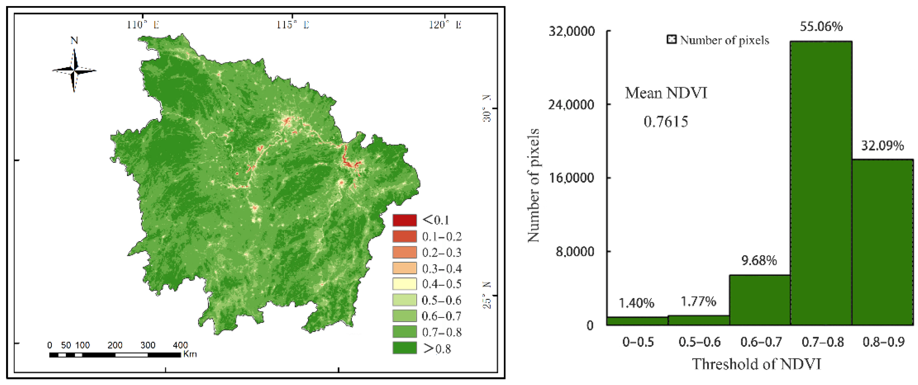
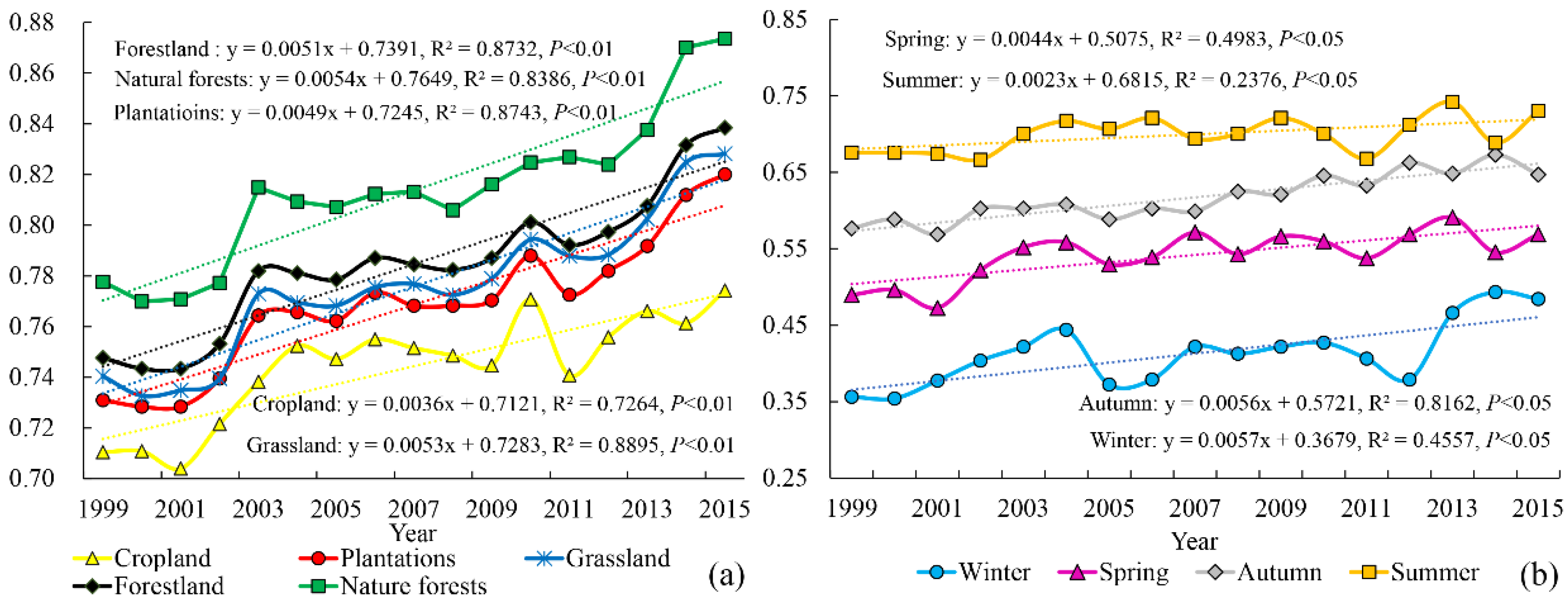
In the past 17 years, the NDVI of vegetation in the MRYR showed an overall upward trend (improvement area accounted for more than 3/4) (Figure 3 and Table 4). This is consistent with the research results of the NDVI change trend of different scales in Hubei Province [69], Hunan Province [70], Jiangxi Province [71], and the Yangtze River Basin [72]. The annual mean NDVI values of the Yangtze River Delta, Pearl River Delta, and other coastal urban agglomerations are mostly between 0.3 and 0.5. Compared with them, the NDVI in the MRYR was relatively high. First, from 2004 to 2005, the climate of each province in the study area was abnormal, which showed that the winter lasted for a long time, the temperature was extremely low, and the phenomenon of “late spring cold” appeared in spring, which led to the extremely poor growth of winter vegetation and the sharp decline of NDVI. Second, from 2010 to 2011, the NDVI of vegetation decreased in all seasons, which was due to the serious impact on vegetation growth caused by the large-scale drought in this year. At the same time, it can be seen that the impact of drought on natural forest has a certain lag and is smaller than other vegetation types, which also shows that the stability of natural forest ecosystems is stronger to a certain extent [73]. The stand structure of mature plantations in China was single and the regulation capacity of the ecosystem was low. The average volume was only 71.55 m³, which is only 41% of mature natural forests. It can be seen that there was still much room for improvement of plantations in the study area, and its ecosystem service function should be improved to ensure the sustainable and healthy growth of plantations.

In addition, different spatial resolutions of NDVI would definitely lead to different research results. In this paper, Landsat images with a resolution of 30 m were used to obtain the boundary of different land uses/land cover, and 1 km NDVI was used to depict the dynamic change of land cover, which had certain limitations. In the future, open resources with a higher resolution such as 250 m and 500 m could be considered, and Landsat images data with a resolution of 30 m could also be used to calculate and obtain NDVI values to further study the vegetation dynamic changes in the middle reaches of the Yangtze River.

Nemani et al. and Liu et al. considered that hydrothermal climate conditions were the driving factors affecting the spatial pattern of land vegetation cover [20,74]. This study showed that relative humidity was the main climatic factor affecting the growth of different vegetation types in the study area in terms of interannual variation, and the partial correlation analysis between relative humidity and NDVI of each vegetation type showed a significant negative correlation. In addition, the correlation between cropland and precipitation was significant (R = 0.149, p < 0.05). This was consistent with the research results regarding the response of vegetation NDVI to climate in east China and its surrounding areas [75,76,77]. The reason for this might be that the precipitation in the study area was rich enough to meet the needs of vegetation growth, and the difference of heat was the main driving factor for the difference of NDVI. The results showed that the sunshine hours in January, August, and December had significant positive effects on the vegetation growth of natural forests, while the rainfall and relative humidity in January, May, August, and December had negative effects on the vegetation growth. NDVI was positively correlated with precipitation in summer and autumn, negatively correlated with precipitation in spring, and positively correlated with sunshine hours. It showed that moderate precipitation could promote the growth of crops, and high humidity would inhibit the growth of crops and vegetation. In addition, each meteorological factor had an obvious lag effect on NDVI. This was consistent with the results confirmed by Bao et al. from global, regional, and other multi-scale studies, and the feedback of vegetation cover on climate change has a certain lag effect [78].

6. Conclusions

With the urbanization process in the MRYR in the past 17 years, on the one hand, the area was greatly disturbed by human activities, with the rapid growth of built-up land and the sharp decline of cropland. On the other hand, the implementation of Chinese ecological protection projects (grain to green, construction of Yangtze River shelterbelt, etc.) and the promulgation of various management policies played a great role in the ecological protection of the MRYR. Forestland is the main part of the land use/cover types (more than 50%), and it was increasing in the period, but it is worth noting that the area of natural forests has decreased (about one tenth), and the proportion of plantations continues to increase. From 1999 to 2015, the vegetation situation in the MRYR gradually improved, especially the natural forests, accounting for 45.39%. The area with an unclear future change trend of plantations accounted for the highest proportion (more than half). According to the relationship between climate factors and vegetation growth, relative humidity had significant negative effects on NDVI (p < 0.05), especially on cropland. On the inter-monthly scale, climate factors (temperature, precipitation, relative humidity, and sunshine hours) had significant lag effects on natural forests and plantations. Sunshine hours promoted vegetation growth positively, while relative humidity had negative effects. Although the overall development trend of forestland in the study area was good, natural forests and plantations were facing problems, respectively. We should protect natural forests and prevent the loss of those with strong ecosystem services and replace those that do not with plantations with a single species diversity.

References

1. Paruelo, J.M.; Epstein, H.E.; Burke, L. ANPP Estimates from NDVI for the Central Grassland Region of the United States. Ecology 1997, 78, 953–958. [Google Scholar]
2. Prăvălie, R. Major perturbations in the Earth’s forest ecosystems. Possible implications for global warming. Earth-Sci. Rev. 2018, 185, 544–571. [Google Scholar] [CrossRef]
3. Zhu, L.; Meng, J.; Zhu, L. Applying Geodetector to disentangle the contributions of natural and anthropogenic factors to NDVI variations in the middle reaches of the Heihe River Basin. Ecol. Indic. 2020, 117, 106545. [Google Scholar] [CrossRef]
4. IPCC. Special Report on Global Warming of 1.5 °C; Cambridge University Press: Cambridge, UK, 2018. [Google Scholar]
5. Gao, J.B.; Jiao, K.W.; Wu, S.H. Investigating the spatially heterogeneous relationships between climate factors and NDVI in China during 1982 to 2013. J. Geogr. Sci. 2019, 29, 1597–1609. [Google Scholar] [CrossRef] [Green Version]
6. Li, T.; Meng, Q. Forest dynamics in relation to meteorology and soil in the Gulf Coast of Mexico. Sci. Total Environ. 2020, 702, 134913.1–134913.11. [Google Scholar] [CrossRef]
7. Li, X.; Liu, H.; Wang, L.; Zhuo, Y. Vegetation Cover Change and Its Relationship Between Climate and Human Activities in Ordos Plateau. Chin. J. Agrometeorol. 2014, 35, 470–476. [Google Scholar]
8. Guan, Q.; Yang, L.; Guan, W.; Wang, F.; Liu, Z.; Xu, C. Assessing vegetation response to climatic variations and human activities: Spatiotemporal NDVI variations in the Hexi Corridor and surrounding areas from 2000 to 2010. Theor. Appl. Climatol. 2019, 135, 1179–1193. [Google Scholar] [CrossRef]
9. Wei, R.; Liu, J.; Zhang, T.; Zhang, Q.; Peng, T.; Liu, Y.L. Spatiotemporal Variation Characteristics of Vegetation in Growing Season and Its Response to Meteorological Factors in Yalong River Basin. J. Ecol. Environ. 2021, 1–11. Available online: http://kns.cnki.net/kcms/detail/44.1661.X.20210201.2128.002.html (accessed on 15 April 2021). (In Chinese).
10. Zhang, Y.L.; Li, L.H.; Ding, M.J.; Zheng, D. Greening of the Tibetan Plateau and its drivers since 2000. Chin. J. Nat. 2017, 39, 173–178. [Google Scholar]
11. Yang, G.S.; Xu, X.B.; Li, P.X. Study on the construction of green ecological corridor in Yangtze River economic belt. Prog. Geogr. Sci. 2015, 34, 1356–1367. [Google Scholar]
12. Yue, J.S. Evaluation of Wetland Ecological Engineering Based on Emergy Theory; Chongqing University: Chongqing, China, 2017. [Google Scholar]
13. Zhao, Q.Q.; Fan, J.W.; Liu, J.Y. Objective based ecological effect evaluation and policy suggestions for the first phase of ecological protection and construction of the three river source. J. Chin. Acad. Sci. 2017, 32, 35–44. (In Chinese) [Google Scholar]
14. Tang, J.; Cao, H.Q.; Chen, J. Quantifying the impacts of ecological protection projects and climate change on vegetation change in the source region of the Yangtze River. Acta Geogr. A Sin. 2019, 74, 76–86. [Google Scholar]
15. FAO. Global Forest Resources Assessment 2015; FAO Forestry Paper No. 1; FAO: Rome, Italy, 2016. [Google Scholar]
16. Central People’s Government of the People’s Republic of China and the State Forestry and Grassland Administration: The Preserved Area of China’s Artificial Forests is 69.33 Million Hectares, Ranking First in the World. 24 October 2018. Available online: http://www.gov.cn/xinwen/2018-10/24/content_5333969.htm (accessed on 15 April 2021).
17. State Forestry and Grassland Administration. Authoritative Release: Notice of the State Forestry Administration on Publishing the Main Results of the Ninth National Forest Resources Inventory in Jilin and Other Seven Provinces (Cities). 24 October 2018. Available online: http://www.forestry.gov.cn/main/72/content-760624.html (accessed on 15 April 2021).
18. Chung, C. Thirty Years of Ecological Engineering with Spartina Plantations in China. Ecol. Eng. 1993, 2, 261–289. [Google Scholar] [CrossRef]
19. Song, W.; Liu, Y.; Tong, X. Newly sequestrated soil organic carbon varies with soil depth and tree species in three forest plantations from northeastern China. For. Ecol. Manag. 2017, 400, 384–395. [Google Scholar] [CrossRef]
20. Liu, M.; Tu, J. The position and role of Wuhan City in the regional economic macro-strategies of China. Chin. Geogr. Ence 1998, 8, 106–116. [Google Scholar] [CrossRef]
21. Seagren, E.G.; Schoenbohm, L.M.; Owen, L.A.; Figueiredo, P.M.; Hammer, S.J.; Rimando, J.M.; Wang, Y.; Bohon, W. Lithology, topography, and spatial variability of vegetation moderate fluvial erosion in the south-central Andes. Earth Planet. Sci. Lett. 2020, 551, 116555. [Google Scholar] [CrossRef]
22. Jiang, S.; Chen, X.; Smettem, K.; Wang, T. Climate and land use influences on changing spatiotemporal patterns of mountain vegetation cover in southwest China. Ecol. Indic. 2021, 121, 107193. [Google Scholar] [CrossRef]
23. Eastman, J.R.; Sangermano, F.; Machado, E.A.; Rogan, J.; Anyamba, A. Global Trends in Seasonality of Normalized Difference Vegetation Index (NDVI), 1982–2011. Remote Sens. 2013, 5, 4799–4818. [Google Scholar] [CrossRef] [Green Version]
24. Liu, Y.; Li, Y.; Li, S.; Motesharrei, S. Spatial and Temporal Patterns of Global NDVI Trends: Correlations with Climate and Human Factors. Remote Sens. 2015, 7, 13233–13250. [Google Scholar] [CrossRef] [Green Version]
25. Ding, Z.H.; Peng, J.; Qiu, S.J.; Zhao, Y. Nearly Half of Global Vegetated Area Experienced Inconsistent Vegetation Growth in Terms of Greenness, Cover, and Productivity. Earth’s Future 2020, 10, 1618. [Google Scholar] [CrossRef]
26. Hill, M.J.; Donald, G.E.; Hyder, M.W.; Smith, R.C. Estimation of pasture growth rate in the south west of Western Australia from AVHRR NDVI and climate data. Remote Sens. Environ. 2004, 93, 528–545. [Google Scholar] [CrossRef]
27. Xu, Y.F.; Yang, J.; Chen, Y.N. NDVI-based vegetation responses to climate change in an arid area of China. Theor. Appl. Climatol. 2016, 126, 213–222. [Google Scholar] [CrossRef]
28. Feng, S.; Fan, F. A Hierarchical Extraction Method of Impervious Surface Based on NDVI Thresholding Integrated with Multispectral and High-Resolution Remote Sensing Imageries. IEEE J. Sel. Top. Appl. Earth Obs. Remote Sens. 2019, 12, 1461–1470. [Google Scholar] [CrossRef]
29. Zhu, Z.; Piao, S.; Myneni, R.B.; Huang, M.; Zeng, Z.Z.; Canadell, J.G.; Ciais, P.; Sitch, S.; Friedlingstein, P.; Arneth, A.; et al. Greening of the earth and its drivers. Nat. Clim. Chang. 2016, 25, 791–795. [Google Scholar] [CrossRef]
30. Xu, Y.F.; Pan, W.S.; Zhang, Y.L. NDVI change in Guizhou Plateau and its response to climate change. Acta Ecol. Sin. 2020, 29, 1507–1518. [Google Scholar]
31. Prăvălie, R.; Sirodoev, I.; Nita, I.; Patriche, C.; Dumitraşcu, M.; Roşca, B.; Tişcovschi, A.; Bandoc, G.; Săvulescu, I.; Manoiu, V.; et al. NDVI-based ecological dynamics of forest vegetation and its relationship to climate change in Romania during 1987–2018. Ecol. Indic. 2022, 136, 108629. [Google Scholar] [CrossRef]
32. Yuan, J.; Xu, Y.; Xiang, J.; Wu, L.; Wang, D. Spatiotemporal variation of vegetation coverage and its associated influence factor analysis in the Yangtze River Delta, eastern China. Environ. Sci. Pollut. Res. 2019, 26, 32866–32879. [Google Scholar] [CrossRef] [PubMed]
33. Li, Z.; Huffman, T.; McConkey, B.; Townley-Smith, L. Monitoring and modeling spatial and temporal patterns of grassland dynamics using time-series MODIS NDVI with climate and stocking data. Remote Sens. Environ. 2013, 138, 232–244. [Google Scholar] [CrossRef]
34. Suzuki, R.; Tanaka, S.; Yasunari, T. Relationships between meridional profiles of satellite-derived vegetation index (NDVI) and climate over Siberia. Int. J. Climatol. 2015, 20, 955–967. [Google Scholar] [CrossRef] [Green Version]
35. Li, P.; Wang, J.; Liu, M.; Xue, Z.; Bagherzadeh, A.; Liu, M. Spatio-temporal variation characteristics of NDVI and its response to climate on the Loess Plateau from 1985 to 2015. Catena 2021, 203, 105331. [Google Scholar] [CrossRef]
36. Yuan, Z.; Yu, Z.Q.; Feng, Z.Y.; Xu, J.J.; Yin, J.; Yan, B.; Lei, H. Spatiotemporal variation of NDVI and its response to water and heat conditions in terrestrial ecosystems of the Yangtze River Basin. Proc. Yangtze River Acad. Sci. 2019, 36, 7–15. [Google Scholar]
37. Yi, Y.; Hu, X.L.; Shi, M.C.; Kang, H.Z.; Wang, B.; Zhang, C.; Liu, C.J. Regional vegetation dynamics in the middle reaches of the Yangtze River Based on MODIS NDVI and its relationship with climate factors. Acta Ecol. Sin. 2021, 41, 7796–7807. [Google Scholar] [CrossRef]
38. Dong, L. Multi model remote sensing estimation of forest leaf area index in Three Gorges Reservoir Area. Land Resour. Remote Sens. 2019, 31, 73–81. [Google Scholar]
39. Haralick, R.M.; Shanmugam, K.; Dinstein, I. Textural features for image classification. IEEE Trans. Syst. Man Cybern. 1973, 6, 610–621. [Google Scholar] [CrossRef] [Green Version]
40. Huang, C.; Zhang, C.; Liu, Q.; Li, H.; Yang, X.; Liu, G. Fine identification of tree species in tropical typical plantation based on multiple features of optical and radar images. For. Sci. 2021, 57, 80–91. [Google Scholar]
41. Brewer, K.; Lottering, R.; Peerbhay, K. Remote sensing of invasive alien wattle using image texture ratios in the low-lying Midlands of KwaZulu-Natal, South Africa. Remote Sens. Appl. Soc. Environ. 2022, 26, 100769. [Google Scholar] [CrossRef]
42. Park, Y.; Guldmann, J.-M. Measuring continuous landscape patterns withGray-Level Co-Occurrence Matrix (GLCM) indices: An alternative to patch metrics? Ecol. Indic. 2020, 109, 105802. [Google Scholar] [CrossRef]
43. Hu, X.L.; Yi, Y.; Kang, H.Z.; Wang, B.; Shi, M.C.; Liu, C.J. Spatial temporal pattern and driving factors of land use change in the middle reaches of the Yangtze River in recent 25 years. Acta Ecol. Sin. 2019, 39, 1877–1886. [Google Scholar]
44. Shi, Y.Y.; Li, M.; Fu, Y.; Wang, L.W.; Sun, M.X.; Hao, J.M. Multi scenario traffic land demand forecasting based on grey BP neural network model: A case study of urban agglomeration in the middle reaches of the Yangtze River. J. China Agric. Univ. 2020, 25, 142–153. [Google Scholar]
45. National Bureau of Statistics of the People’s Republic of China. China Statistical Yearbook—2016; China Statistics Press: Beijing, China, 2016. [Google Scholar]
46. China’s National Standard (GB/T 21010—2017). Current Land Use Condition Classification. Available online: http://www.gov.cn/xinwen/2017-11/04/content_5237211.htm (accessed on 1 November 2021).
47. Tao, S.; Guang, T.T.; Peng, W.P.; Wang, G.J. Spatiotemporal changes and driving forces of NDVI in the upper reaches of the Yangtze River from 2000 to 2015: A case study of Yibin City. Acta Ecol. Sin. 2020, 40, 5029–5043. [Google Scholar]
48. Baraldi, A.; Parmiggiani, F. Investigation of the textural characteristics associated with gray level cooccurrence matrix statistical parameters. IEEE Trans. Geosci. Remote Sens. 1995, 33, 293–304. [Google Scholar] [CrossRef]
49. Wang, P.; Qiao, H.; Zhang, Y.; Li, Y.; Feng, Q.; Chen, K. Meso-damage evolution analysis of magnesium oxychloride cement concrete based on X-CT and grey-level co-occurrence matrix. Constr. Build. Mater. 2020, 255, 119373. [Google Scholar] [CrossRef]
50. Priyanka; Dharmender, K. Feature Extraction and Selection of kidney Ultrasound Images Using GLCM and PCA. Procedia Comput. Sci. 2020, 167, 1722–1731. [Google Scholar] [CrossRef]
51. Zhang, G. Spatial distribution of urban forest carbon storage in Shanghai based on remote sensing estimation. J. Ecol. Environ. 2021, 30, 1777–1786. (In Chinese) [Google Scholar] [CrossRef]
52. Hlatshwayo, S.T.; Mutanga, O.; Lottering, R.T.; Kiala, Z.; Ismail, R. Mapping forest aboveground biomass in the reforested Buffelsdraai landfill site using texture combinations computed from SPOT-6 pan-sharpened imagery. Int. J. Appl. Earth Obs. Geoinf. 2019, 74, 65–77. [Google Scholar] [CrossRef]
53. Poona, N. Invasive alien plant species in South Africa: Impacts and management options. Alternation 2008, 15, 160–179. [Google Scholar]
54. Lottering, R.; Mutanga, O.; Peerbhay, K.; Ismail, R. Detecting and mapping Gonipterus scutellatus induced vegetation defoliation using WorldView-2 pan-sharpened image texture combinations and an artificial neural network. J. Appl. Remote Sens. 2019, 13, 014513. [Google Scholar] [CrossRef]
55. Sen, K.P. Estimates of the regression coefficient based onKendall’s tau. J. Am. Stat. Assoc. 1968, 63, 1379–1389. [Google Scholar] [CrossRef]
56. Sun, Y.J.; Liu, X.F.; Ren, Z.Y.; Duan, Y.F. Spatial and temporal variation characteristics of drought and heat wave in the Loess Plateau from 1960 to 2016. Adv. Geogr. Sci. 2020, 39, 591–601. [Google Scholar]
57. Kendall, M.G. Rank correlation methods. Br. J. Psychol. 1990, 25, 86–91. [Google Scholar] [CrossRef]
58. Mann, H.B. Non-parametric test against trend. Econometrica 1945, 13, 245–259. [Google Scholar] [CrossRef]
59. Tong, S.; Zhang, J.; Bao, Y.; Lai, Q.; Lian, X.; Li, N.; Bao, Y. Analyzing vegetation dynamic trend on the Mongolian Plateau based on the Hurst exponent and influencing factors from 1982–2013. J. Geogr. Sci. 2018, 28, 595–610. [Google Scholar] [CrossRef] [Green Version]
60. Kalisa, W.; Igbawua, T.; Henchiri, M.; Ali, S.; Zhang, S.; Bai, Y.; Zhang, J.H. Assessment of climate impact on vegetation dynamics over East Africa from 1982 to 2015. Sci. Rep. 2019, 9, 16865. [Google Scholar] [CrossRef] [PubMed] [Green Version]
61. Hurst, F.B. Climates prevailing in the yellow-gray earth and yellow-brown earth zones in New Zealand. Soil Sci. 1951, 72, 1–20. [Google Scholar] [CrossRef] [Green Version]
62. Mandelbrot, B.B.; Wallis, J.R. Robustness of the rescaled range R/S in the measurement of noncyclic long run statistical dependence. Water Resour. Res. 1969, 5, 967–988. [Google Scholar] [CrossRef]
63. Sun, Y.; Chen, S.H.; Su, H.B. Spatial and temporal variation of NDVI in different ecological types of the Loess Plateau and its response to climate change. Geogr. Res. 2020, 39, 1200–1214. [Google Scholar]
64. Ye, C.S.; Dong, Y.X. Fractal characteristics of land use and its influencing mechanism in Pearl River Delta. J. Agric. Eng. 2011, 27, 330–335. [Google Scholar]
65. Zhao, Y.L.; Liu, Y.Z.; Long, K.S. Analysis on characteristics and influencing factors of urban land development intensity in Yangtze River Delta. Resour. Environ. Yangtze River Basin 2012, 21, 1480–1485. [Google Scholar]
66. Su, S.; Zhou, X.; Wan, C.; Li, Y.; Kong, W. Land use changes to cash crop plantations: Crop types, multilevel determinants and policy implications. Land Use Policy 2016, 50, 379–389. [Google Scholar] [CrossRef]
67. Guo, F.; Wang, H.R.; Li, X. Food security War: Guarantee supply, cultivated land, environment and talents. China Econ. Wkly. 2013, 25, 26–31. [Google Scholar]
68. Xue, W.X. Problems and Countermeasures of Plantation Quality in China. Mod. Hortic. 2015, 9, 99–100. [Google Scholar]
69. Yuan, M.X.; Zou, L.; Lin, A.W.; Zhu, H.J. Analyzing dynamic vegetation change and response to climatic factors in Hubei Province, China. Acta Ecol. Sin. 2016, 36, 5315–5323. [Google Scholar]
70. Liu, Z.C.; Qu, Y.Y. Vegetation change and its response to climate change in Hunan Province Based on spot-vgt data. J. Beijing For. Univ. 2019, 41, 84–91. [Google Scholar]
71. Yin, S.J.; Chen, X.L.; Wu, C.Q.; Yao, Y.J.; Wang, X.L. Analysis of temporal and spatial changes of vegetation cover in Jiangxi Province Based on NDVI. J. Cent. China Norm. Univ. 2013, 47, 129–135. [Google Scholar]
72. Li, Y. Vegetation Cover and Changes of Agricultural Biomass in the Yangtze River Basin in Recent 20 Years Based on NDVI; Peking University: Beijing, China, 2004. [Google Scholar]
73. Zhang, J.M.; Ju, J.L.; Li, Z.X. Interannual variation of agricultural drought in Hunan Province and prediction of severe disaster years. J. Nat. Disasters 2011, 20, 105–110. [Google Scholar]
74. Nemani, R.R.; Keeling, C.D.; Hashimoto, H.; Jolly, W.M.; Piper, S.C.; Tucker, C.J.; Myneni, R.B.; Running, S.W. Climate-driven increases in global terrestrial net primary production from 1982 to 1999. Science 2003, 300, 1560–1563. [Google Scholar] [CrossRef] [Green Version]
75. Li, B.G.; Tao, S. Correlation analysis between AVHRR NDVI and climatic factors. Acta Ecol. Sin. 2000, 20, 898–902. [Google Scholar]
76. Chen, Y.H.; Li, X.B.; Shi, P.J. Analysis of climatic factors driving NDVI change in China during 1983-1992. Acta Phytoecol. Sin. 2001, 25, 716–720. [Google Scholar]
77. Yu, Z.L.; Qin, T.L.; Zhang, S.Y.; Shi, W.L. Study on the change law of vegetation index and the influence of climate factors in the Yangtze River Basin in recent years. J. China Acad. Water Resour. Hydropower Sci. 2016, 14, 362–366, 373. [Google Scholar]
78. Bao, G.; Bao, Y.; Sanjjava, A.; Qin, Z.; Zhou, Y.; Xu, G. NDVI-indicated long-term vegetation dynamics in Mongolia and their response to climate change at biome scale. Int. J. Climatol. 2016, 35, 4293–4306. [Google Scholar] [CrossRef]
Figure 1. The location of MRYR in China. (ac) plantations in the study areas; (df) natural forests in the study areas.
Forests 13 01224 g001
Figure 2. Flow chart of the main steps of dynamic changes of plantations and natural forests in study area and their relationship with climatic factors.
Forests 13 01224 g002
Figure 3. The Land use/cover types in the MRYR from 1999 to 2015.
Forests 13 01224 g003
Figure 4. Spatial distribution of mean NDVI and pixel distribution in the MRYR from 1999 to 2015.
Forests 13 01224 g004
Figure 5. Variations of NDVI in the MRYR from 1999 to 2015. (a) mean NDVI of different vegetation in different years; (b) mean NDVI of all vegetation in different seasons.
Forests 13 01224 g005
Figure 6. Distribution and variation of NDVI in plantations (ac) and natural forests (df) in the MRYR.
Forests 13 01224 g006