Development of a Climate-Sensitive Matrix Growth Model for Larix gmelinii Mixed-Species Natural Forests and Its Application for Predicting Forest Dynamics under Different Climate Scenarios

Abstract

Larix gmelinii natural forests, which are of great ecological and economic importance, are mainly distributed in northeast China. Sustainable management of these forests play a vital role in ecological security in northeast China, especially in the context of climate change. Forest growth models, which support forest management decision-making, are lacking for Larix gmelinii natural forests, hampering the prescription of forest management strategies. In this study, we produced a climate-sensitive, transition-matrix model (CM) for Larix gmelinii natural forests. For comparison, a variable transition model without including climate change effects (NCM) and a fixed-parameter model (FM) were also built. We examined the performance of the CM, NCM, and FM by conducting short- (5 years) and long-term (100 years) simulations. The results showed that for short-term prediction, no significant difference was observed among the three predictive models. However, the long-term prediction ability of the CM under the three different RCPs was superior to that of the FM and NCM. The number of trees and basal area were predicted to increase under climate change, which might result in natural disasters, such as snow break, windthrow, and forest fire. Silvicultural practices, such as reducing the intermediate thinning interval and the enrichment planting of slow-growing trees, should be implemented to mitigate the deleterious effects of climate change.

1. Introduction

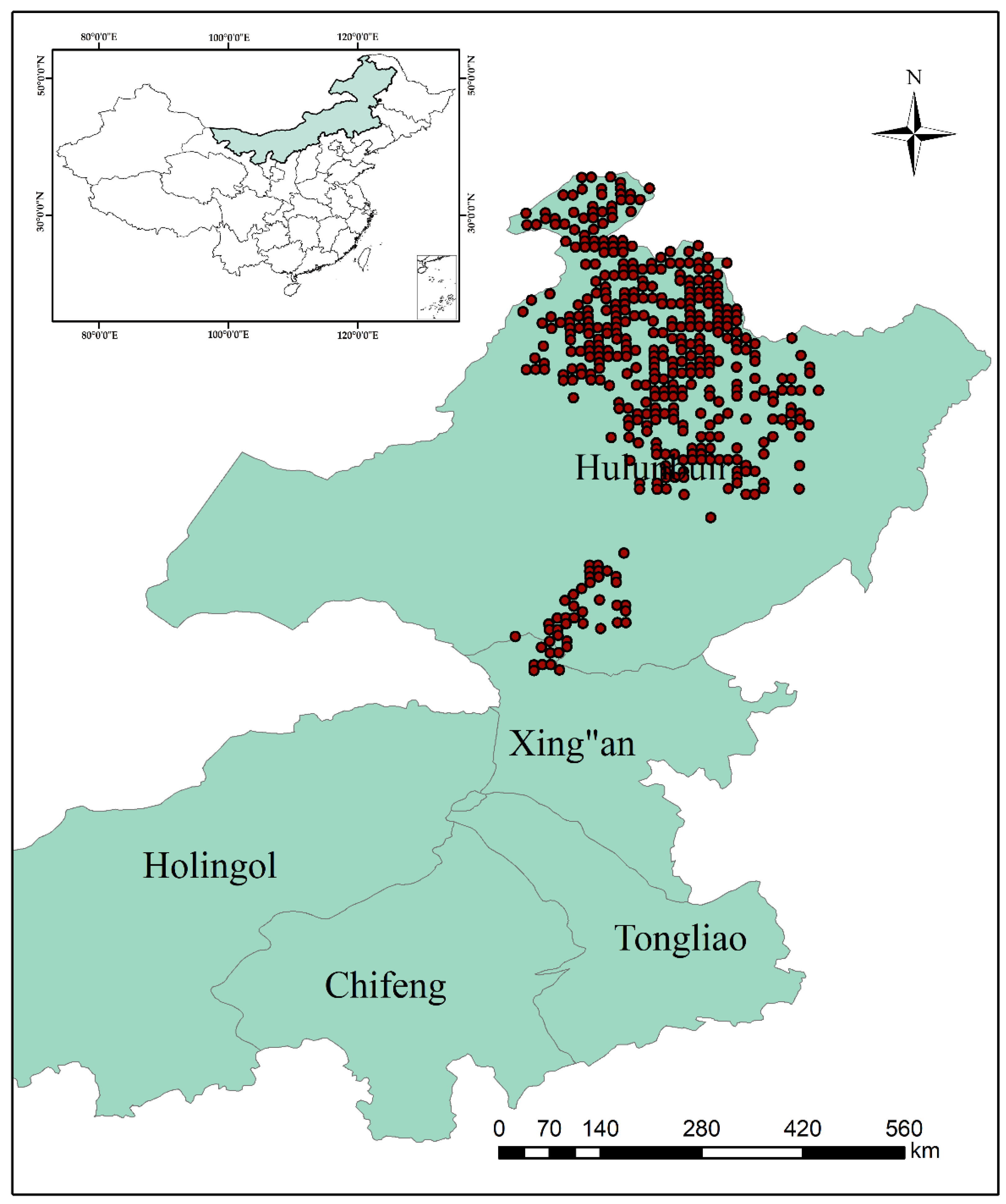
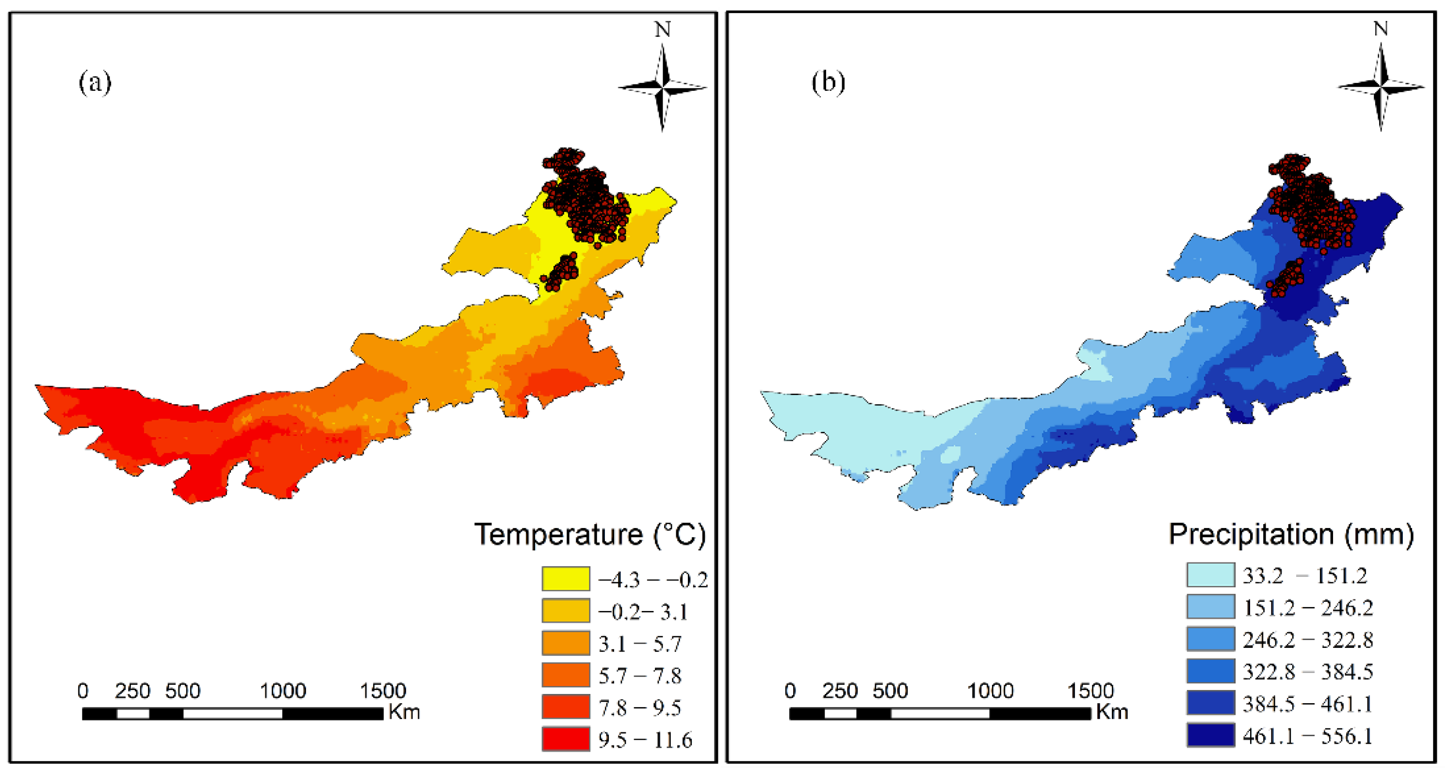
Larix gmelinii natural forests are a typical vegetation community in the Xing’an Mountains area in northeast China [1,2,3]. They cover an area of 40,421 ha with a stocking of 4,654,312 m³, representing 49% of the total forest area and 49% of stocking in the Xing’an Mountains [4]. It is noteworthy that they are distributed in the southern edge of the global northern coniferous forest range and hence play a vital role in ecological security for northeast China [5,6]. Larix gmelinii is also of economic importance and is widely used for furniture, construction, and shipbuilding because of its toughness [7,8].

Like other natural forests, Larix gmelinii natural forests have been suffering from deforestation and degradation due to the old forest policy (1950–1997) in China, which was designed to maximize timber production for economic development. Zhang [9] documented that from 1950 to 1995 natural forests declined to 30% of the total forest area in China and the unit-area stocking of natural forests decreased by 32%. In 1998, China established Natural Forest Conservation Program (NFCP), articulating the new forest policy, which focused on forest ecological services other than wood production [9,10]. In 2017, China further banned all commercial logging in natural forests [11] and encouraged scientific forest management strategies for forest restoration [12].

Formulating forest management strategies requires accurate prediction and comparison of forest growth and yield under different management scenarios [13,14]. Forest growth models plays an important role in prescribing forest management strategies. For instance, Sterba [15] employed the distance-independent individual tree growth model PROGNAUS to determine the equilibrium curve for mixed-species forests in Austria. Lars, et al. [16] used a single-tree growth model to investigate the possibility of transforming normal, young Norway spruce forests to develop more heterogeneous stand structures, aiming for multi-layered forests in the long run. Normally, forest growth models are categorized into whole-stand models, size-class models, and individual-tree models according to the relevant modeling units [17]. The whole stand model cannot capture variability regarding individual tree size and species, resulting in incapability of predicting forest dynamics with complex forest structures [18]. Tree size-class models and individual-tree models, which employ a finer modeling resolution, i.e., diameter class and individual tree, respectively, are used to assess more complex species compositions and structures [18,19].

Individual-tree models use an individual tree as the modeling unit and are thus capable of a better mimicking of reality and integrating spatial heterogeneity [17,20]. However, they are challenging to develop as they require large amounts of individual tree-level data, which is especially the case for distance-dependent individual-tree models [14,17]. By comparison, tree-size models are easier to develop and have shown robust performance in modeling forest dynamics of unevenly aged, mixed-species forests [18,21].

As the largest terrestrial ecosystem type, forests play a significant role in combating climate change by absorbing CO₂. As much as 30% (2 petagrams of carbon per year; Pg C year−C) of annual global anthropogenic CO₂ emissions are sequestrated by the world’s forests [22,23]. Climate change, in turn, can also influence forest productivity [24,25], tree mortality [26,27,28], and tree recruitment [29,30], and hence plays a vital role in shaping forest structure and species composition [31,32]. The aims of our present study were to produce a climate-sensitive transition-matrix forest growth model (CM) by integrating climate variables for Larix gmelinii natural forests. With the new CM, we simulated forest dynamics under varying climate change scenarios. Based on the results of the simulations, we propose some silvicultural practices that could be implemented to mitigate the negative effects of climate change.

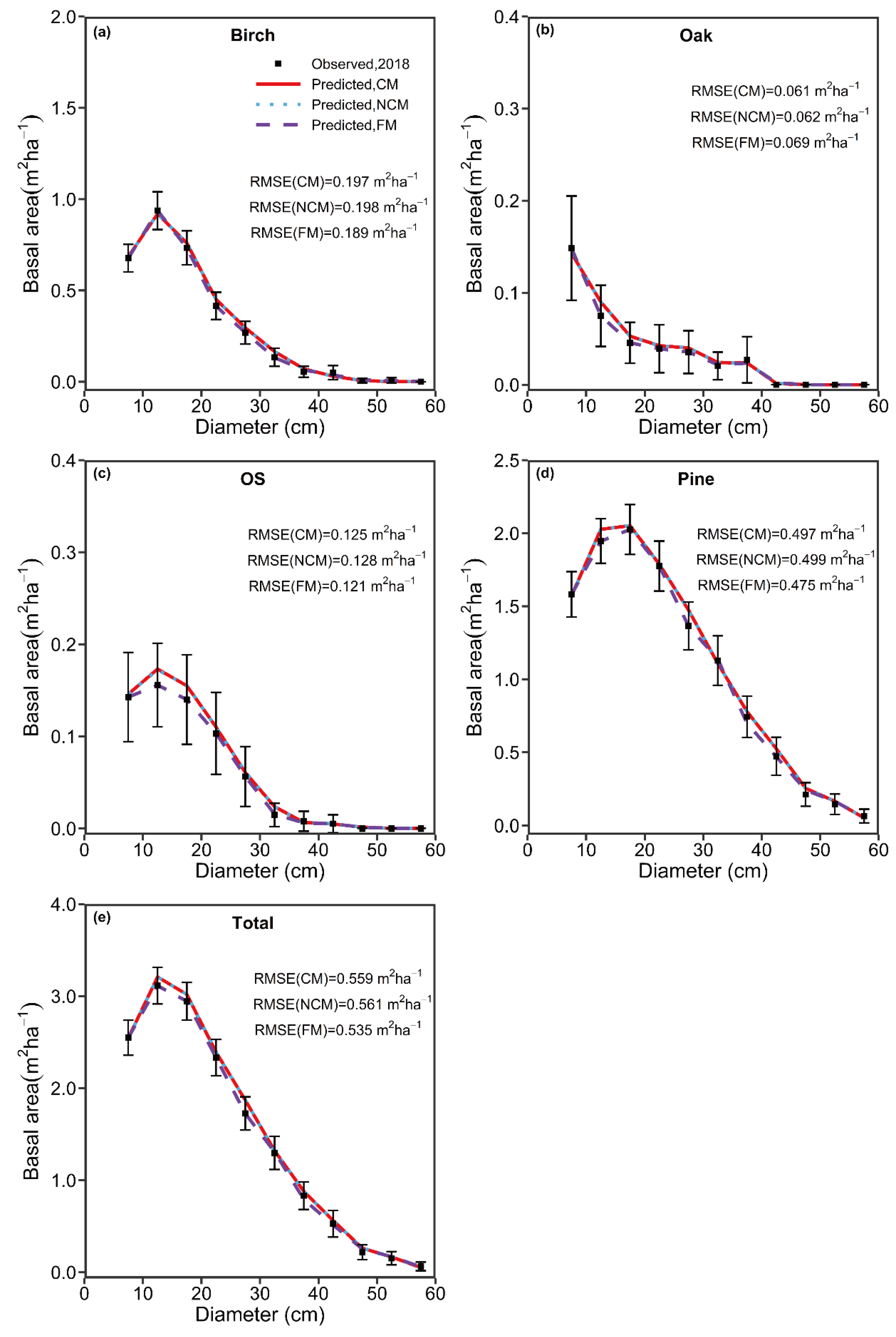
2. Materials and Methods

2.1. Study Area and Data

The study area is located in the state-owned forest region of the Greater Khingan Mountains in the northeastern region of Inner Mongolia (119°36′20″–125°20′50″ E, 46°08′40″–53°20′00″ E) (Figure 1). It is ~696 km from north to south and 384 km east to west. It is the largest state-owned forest region in China, with an average forest coverage of 80.5%. The altitude ranges from 425 m to 1760 m. The annual average temperature is −2–−4 °C with a maximum temperature of 37.5 °C and a minimum temperature of −52 °C. The average annual rainfall is ~450 mm, 80% of which is concentrated from July to August.

The plots for Larix gmelinii natural forests used for model development were selected from the eighth (2013) and ninth (2018) national forest inventory (NFI) in this region. The sample plots had an area of 0.067 ha, layed out in a grid of 8 × 8 km (Figure 1). Plots with evident disturbances, for instance, logging or artificial enrichment were excluded. Finally, a total of 428 plots with 48,069 individual observations were selected. In each plot, individual tree and plot variables were recorded. The individual-tree variables consisted of tree number, species name, and diameter at breast height (DBH). The plot variables included slope, aspect, slope position, elevation, average DBH, and canopy density.

2.2. Methods

2.2.1. Data Pre-Analysis

In Larix gmelinii natural forests, other tree species include Betula platyphylla, Betula costata, Quercus mongolica, Pinus sylvestris, and Salix spp. Larix gmelinii and Pinus sylvestris are in the pine family. These tree species were categorized into 4 species classes, i.e., birch, oak, pine, and softwoods for model development and detailed information about the categorization are shown in

Table 1. The main tree species identified and their frequency in the sample plots.

Species Class	Main Tree Species	Species Frequency	Species Class Frequency
Birch	Betula platyphylla	25.55%	26.36%
	Betula costata	0.82%
Softwood	Salix spp.	0.50%	5.13%
	other softwood	4.62%
Oak	Quercus mongolica	3.60%	3.60%
Pine	Larix gmelinii	64.22%	64.91%
	Pinus sylvestris	0.69%

. The descriptive statistics of plots and individual tree characteristics were calculated and are provided in

Table 2. Summary of plot data. Number of trees (N), quadratic mean DBH, basal area, size diversity, and species diversity were derived from the first inventory. Tree recruitment was produced from two inventories.

	N (Trees ha−1)				Quadratic Mean DBH	Basal Area
	Birch	Oak	Softwood	Pine	(cm)	(m2 ha−1)
Mean	268.98	36.76	52.29	662.24	14.20	14.67
SD	266.30	147.91	144.01	438.11	4.24	7.20
Max	1260	1020	1365	3255	32.31	35.39
Min	0	0	0	15	7.50	0.07
	Recruitment (Trees ha−1)				Species Diversity	Size Diversity
	Birch	Oak	Softwood	Pine
Mean	22.78	8.52	10.41	55.76	0.49	1.46
SD	48.14	44.16	58.64	90.33	0.35	0.37
Max	450	540	825	795	1.34	2.26
Min	0	0	0	0	0.00	0.00

and

Table 3. Summary of individual trees. The diameter was recorded in the first inventory. Tree mortality rate and diameter increment were derived from the two inventories; n represents the total number of observations.

	Birch	Oak	Softwood	Pine
Diameter (cm)
Mean	10.62	9.22	10.59	12.07
SD	5.18	5.29	5.20	7.37
Max	53.20	38.90	43.70	73.30
Min	5.00	5.00	5.00	5.00
n	7268	1002	1261	18,225
Diameter increment (cm)
Mean	0.61	0.52	0.97	0.75
SD	0.59	0.43	0.78	0.74
Max	5.00	3.50	5.90	9.60
Min	−4.20	−2.50	−1.10	−4.10
n	7268	1002	1261	18,225
Mortality rate
Mean	0.05	0.04	0.15	0.04
SD	0.22	0.21	0.36	0.19
Max	1.00	1.00	1.00	1.00
Min	0.00	0.00	0.00	0.00
n	7675	1049	1492	18,896

.

2.2.2. Climate Variables

Two climate variables, i.e., mean annual temperature (MAT) and mean annual precipitation (MAP), are extensively used to examine the climate change effects on forest ecosystems [14,33,34]. In this study, the MAT and MAP were calculated using the software, i.e., ClimateAP, which can provide local future and historical climate information for a specific site in the Asia Pacific [35]. The maps for MAT and MAP were produced in the state-owned forest region of the Greater Khingan Mountains (Figure 2).

ClimateAP was further employed to predict monthly precipitation and temperature between 2015 and 2100 to investigate the long-term effects of climate change on the forest ecosystem. The future climate scenarios were produced by the general circulation model (GCM), which was derived from the second generation Canadian Earth System Model (CanESM2) [36,37].

The three representative concentration pathways (RCPs), i.e., RCP2.6, RCP4.5, and RCP8.5, were used to represent the latest climate-change scenarios [38]. More detailed information about RCPs is provided in previous studies [14,38,39].

Future MAT and MAP trends were generated and are shown in Figure 3. In general, the future MAT increased under three RCPs from 2010 to 2100 (Figure 3a). Similarly, the MAP under three RCPs also increased, although fluctuations are predicted (Figure 3b).

2.2.3. Model Development

The transition matrix growth model can be described as follows:

$$y_{t+1}=G_t\left(y_t-h_t\right)+R_t+{ϵ}_t$$

(1)

where y_t = [y_ijt] represents a column vector denoting the number of trees alive in species group i (i = 1, 2, 3, …, sp.) and diameter class j (j = 1, 2, 3, …, dc) at time t; y_t is a space and time-dependent column vector influenced by forest dynamics and logging. h_t = [h_ijt] represents the amount of trees logged in species group i and diameter class j at time t, and h_t = 0 in case of no logging at time t; the growth matrix G_t describes how individual trees grow or die between t and t + 1; R_t denotes the amount of trees recruited in the smallest diameter class for each species group, between t and t + 1; ϵ_t denotes a vector of random errors.

The G and R matrices are:

$$\begin{array}{c}G=\left[\begin{array}{cccc}{G}_1& & & \\ & G_2& & \\ & & \ddots & \\ & & & G_m\end{array}\right]\mathbf{,}{\mathbf{G}}_i=\left[\begin{array}{ccccc}{\alpha }_{i1}& & & & \\ b_{i1}& {\alpha }_{i2}& & & \\ & \ddots & \ddots & & \\ & & b_{i,n-2}& {\alpha }_{i,n-1}& \\ & & & b_{i,n-1}& {\alpha }_{in}\end{array}\right]\\ \mathbf{R}=\left[\begin{array}{c}{R}_1\\ R_2\\ ⋮\\ R_m\end{array}\right]\mathbf{,}{R}_i=\left[\begin{array}{c}{R}_i\\ 0\\ ⋮\\ 0\end{array}\right]\end{array}$$

(2)

where α_ij is the probability of a tree in species group i and diameter class j being alive and still in the original diameter class j in between t and t + 1; m and n represents the number of species groups and diameter classes; b_ij denotes the probability of a tree staying alive and growing into the next diameter class j + 1 in species group i and diameter class j.

Variable α_ij and variable b_ij are related by the following formula:

$$a_{ij}=1-b_{ij}-m_{ij}$$

(3)

where m_ij represents the probability of tree mortality in species group i and diameter class j between t and t + 1.

R_i is defined as a time- and climate-dependent recruitment vector showing the number of trees entering the smallest diameter class of each species, between t and t + 1. The most important step for developing a transition matrix growth model is to define three key variables, i.e., α_ij, b_ij, and m_ij. These three variables were estimated using forest stand and site attributes. The b_ij probability could be derived through dividing the annual tree diameter increment, g_ij, by the diameter class width. Because g_ij could be affected by stand and site attributes, it could thus be expressed as a function of site and stand attributes; g_ij is calculated as follows:

$$\begin{gathered} \log (g_{ij}+1)={\gamma }_{i1}+{\gamma }_{i2}·D_j+{\gamma }_{i3}·D_j{}^2+{\gamma }_{i4}·B+{\gamma }_{i5}·H_1+{\gamma }_{i6}·H_2+{\gamma }_{i7}·MAT \\ +{\gamma }_{i8}·MAP+{\gamma }_{i9}·H+{\gamma }_{i10}·SLCos+{\mu }_{ij} \end{gathered}$$

(4)

where D_j denotes diameter (cm); B is the basal area of a stand (m²·ha⁻¹); H₁ and H₂ represent Shannon’s diversity indices; H₁ indicates species diversity represented by the Shannon–Wiener index; H₂ denotes tree size diversity represented by the Shannon–Wiener index; MAT denotes mean annual temperature (°C); MAP represents mean annual precipitation (mm); H represents Humus thickness; SLCos denots Slope × cos(Aspect) [40]; γ_s are parameters; μ_ij is the error. A generalized least squares (GLS) method was used to estimate the parameters of the tree diameter increment model (Equation (4)).

A tobit model [41] was used to estimate the trees recruited for species group i from t to t + 1, since the trees recruited show a continuous, skewed, bounded, and non-normal pattern, which is truncated to positive values and zeros [14,42]. The tobit model is as follows:

$$R_i=\mathsf{\Omega }\left(\frac{{\beta }_i{x}_i}{{\sigma }_i}\right){\beta }_i{x}_i+{\sigma }_i\omega \left(\frac{{\beta }_i{x}_i}{{\sigma }_i}\right).$$

(5)

$$\begin{gathered} {\beta }_i{x}_i={\beta }_{i1}+{\beta }_{i2}·N_i+{\beta }_{i3}·B+{\beta }_{i4}·H_1+{\beta }_{i5}·H_2+{\beta }_{i6}·MAT+{\beta }_{i7}·MAP+{\beta }_{i8}·H \\ +{\beta }_{i9}·SLCos+v_i \end{gathered}$$

(6)

where N_i represents the amount of trees per unit area (ha) in species group i; Ω and ω denote, respectively, the standard normal cumulative and density functions; σ_i is the standard deviation of the residuals v_i acquired in estimating parameter β. The tobit recruitment Equation parameters (7) were estimated with the maximum likelihood (ML) method.

A probit model was employed to indicate the probability of tree mortality per year, m_ij, that is also expressed as a function of D_j, H₁, H₂, MAT, MAP, H and SLCos. The formula for m_ij is:

$$\begin{gathered} m_{ij}=\frac{M_{ij}}{T}=\frac{1}{T}\mathsf{\Omega }\left({\delta }_{i1}+{\delta }_{i2}·D_j+{\delta }_{i3}·B+{\delta }_{i4}·H_1+{\delta }_{i5}·H_2+{\delta }_{i6}·MAT+{\delta }_{i7}·MAP \\ +{\delta }_{i8}·H+{\delta }_{i9}·SLCos+{\xi }_{ij}\right) \end{gathered}$$

(7)

where M_ij is the probability of a tree in species i and diameter class j dying within T years; δ_s denotes parameters; ξ_ij represents the error. The parameters, δ_s, were estimated using the ML method.

We selected the predictive variables based on three criteria, i.e., the expected biological responses, the statistical significance, and parsimony, to avoid compromised type-I error rates and other artifacts [14,43,44].

2.2.4. Model Validation and Comparison

Ten-fold cross-validation was conducted to investigate the predictive performance of the CM. In ten-fold cross-validation, the data are first partitioned into 10 equally (or nearly equally) sized folds. Next, 10 iterations of model development and validation are performed such that within each iteration a different fold of the data is held out for validation while the remaining 9 folds are used for model development. We calculated the following cross-validated lack-of-fit statistics, i.e., R², RMSE, and MAE, for validation. The formulas are:

$${\mathrm{R}}_{\mathrm{CV}}^2=\frac{1}{\mathrm{k}}{\displaystyle \sum }_{j=1}^{\mathrm{k}}({\mathrm{R}}_j^2)=\frac{1}{\mathrm{k}}{\displaystyle \sum }_{j=1}^{\mathrm{k}}\left(1-\frac{{{\displaystyle \sum }}_{i=1}^{{\mathrm{n}}_j}{\left({\mathrm{O}}_{ij}-{\mathrm{P}}_{ij}\right)}^2}{{{\displaystyle \sum }}_{i=1}^{{\mathrm{n}}_j}{\left({\mathrm{O}}_{ij}-\overline{{\mathrm{O}}_j}\right)}^2}\right)$$

(8)

$${\mathrm{RMSE}}_{\mathrm{CV}}=\frac{1}{\mathrm{k}}{\displaystyle \sum }_{j=1}^{\mathrm{k}}({\mathrm{RMSE}}_j)=\frac{1}{\mathrm{k}}{\displaystyle \sum }_{j=1}^{\mathrm{k}}\left(\sqrt{\frac{1}{{\mathrm{n}}_j}{\displaystyle \sum }_{i=1}^{{\mathrm{n}}_j}{\left({\mathrm{O}}_{ij}-{\mathrm{P}}_{ij}\right)}^2}\right)$$

(9)

$${\mathrm{MAE}}_{\mathrm{CV}}=\frac{1}{\mathrm{k}}{\displaystyle \sum }_{j=1}^{\mathrm{k}}({\mathrm{MAE}}_j)=\frac{1}{\mathrm{k}}{\displaystyle \sum }_{j=1}^{\mathrm{k}}\left(\sqrt{\frac{1}{{\mathrm{n}}_j}{\displaystyle \sum }_{i=1}^{{\mathrm{n}}_j}\left|{\mathrm{O}}_{ij}-{\mathrm{P}}_{ij}\right|}\right)$$

(10)

where k is equal to 10; O_ij is the ith observed value in the jth fold; P_ij represents the ith estimated value in the jth fold; $\overline{{\mathrm{O}}_j}$ is the mean observed value in the jth fold; nj denotes the number of observations in the jth fold; ${\mathrm{R}}_j^2$, RMSE_j, and MAE_j represent the R², RMSE, and MAE in the jth folder.

To examine the performance of CM, we also produced an NCM and a fixed-parameter matric model (FM) using the same 428 sample plots. The FM is the original form of the matrix model in forestry and assumes that forest dynamics are independent of site condition, stand competition, and time-dependent climate variables [18,45]. Thus, the transition probabilities of survivorship, growth, and mortality are assumed to be constant over time [14]. The detailed information about NCM (

Table A1. The estimated parameters with lack-of-fit statistics for the tree diameter increment model of NCM. The dependent variable, diameter increment, was measured in centimeters per five years.

	Birch	Oak	Softwood	Pine
Intercept	9.48 × 10−2 **	9.32 × 10−2	3.10 × 10−1 *	2.05 × 10−1 ***
DBH	5.03 × 10−2 ***	3.27 × 10−2 ***	9.87 × 10−2 ***	6.93 × 10−2 ***
DBH2	−1.05 × 10−3 ***	−9.50 × 10−4 ***	−1.94 × 10−3 ***	−1.26 × 10−3 ***
BA	−3.08 × 10−2 ***	−2.04 × 10−2 ***	−4.40 × 10−2 ***	−4.69 × 10−2 ***
H1	2.91 × 10−1 ***	−8.17 × 10−3	4.08 × 10−1 ***	6.29 × 10−1 ***
H2	8.55 × 10−2 ***	−1.32 × 10−1	−3.81 × 10−2	7.76 × 10−2 ***
Dg	2.79 × 10−2 ***	5.72 × 10−2 ***	2.54 × 10−2 **	7.37 × 10−3 ***
SLcosASP a	−2.40 × 10−3 **	3.49 × 10−3	3.95 × 10−3	−1.04 × 10−2 ***
ST	−1.45 × 10−3 **	3.74 × 10−3 **	2.74 × 10−3	5.70 × 10−3 ***
HT	1.44 × 10−3	1.34 × 10−2 *	−5.12 × 10−3	1.06 × 10−2 ***
R2 b	0.13	0.11	0.15	0.19
AIC	12,131.66	1110.04	2807.75	38,840.45
BIC	12,207.47	1164.04	2864.29	38,926.36
logLik c	−6054.832	−544.02	−1392.88	−19,409.22
df d	7258	992	1251	18,215

Level of significance: * p < 0.10; ** p < 0.05; *** p < 0.01. ^a SLCos = Slope × cos (Aspect). ^b R²: Nagelkerke’s pseudo r-squared. ^c logLik: log-likelihood value. ^d df: Degrees of freedom in model fitting.

,

Table A2. The estimated parameters with the lack-of-fit statistics for the recruitment model of NCM. The dependent variable, recruitment, was derived in units of trees per hectare every five years.

	Birch	Oak	Softwood	Pine
Intercept	−9.73 × 101 ***	−5.73 × 102 ***	−5.22 × 102 ***	1.27 × 102 ***
N	7.27 × 10−2 ***	5.76 × 10−1 ***	3.40 × 10−1 ***	7.18 × 10−2 ***
BA	−5.46 × 100 ***	−6.88 × 100 **	−1.49 × 101 ***	−6.48 × 100 ***
H1	8.05 × 101 ***	1.38 × 102 **	2.45 × 102 ***	5.19 × 101 **
H2	3.85 × 101 **	6.54 × 101	1.21 × 102 *	2.49 × 101
Dg	2.17 × 100	1.15 × 101 **	5.22 × 100	−7.47 × 100 ***
SLcosASP	−8.36 × 10−1	5.40 × 100 **	4.43 × 100 *	−1.19 × 100
ST	4.34 × 10−2	−7.50 × 10−1	2.35 × 100 *	−2.77 × 10−1
HT	1.96 × 100	1.27 × 101 **	2.05 × 100	−3.20 × 10−1
logSigma a	4.37 × 100 ***	4.92 × 100 ***	5.26 × 100 ***	4.64 × 100 ***
R2	0.14	0.32	0.16	0.24
AIC	2485.09	511.45	885.86	3716.77
BIC	2525.68	552.04	926.45	3757.36
logLik	−1232.55	−245.73	−432.93	−1848.39
N b	191,428	33,428	54,428	290,428

Level of significance: * p < 0.10; ** p < 0.05; *** p < 0.01. ^a log sigma: log of the standard deviation of residuals. ^b n: number of plots with recruitment, the total number of plots.

and

Table A3. The estimated parameters with the lack-of-fit statistics for the mortality equations of the NCM. The dependent variable, mortality, equals one if a tree died between the two inventories, if not, it equals zero.

	Birch	Oak	Softwood	Pine
Intercept	−1.83 × 100 ***	−2.90 × 100 ***	−1.29 × 100 ***	−2.35 × 100 ***
DBH	−1.01 × 10−1 ***	7.14 × 10−2	−9.12 × 10−2 ***	−5.60 × 10−2 ***
DBH2	2.60 × 10−3 ***	−1.84 × 10−3	1.47 × 10−3	8.71 × 10−4 ***
BA	2.47 × 10−2 ***	4.79 × 10−2 **	3.09 × 10−3	1.70 × 10−2 ***
H1	−7.77 × 10−2	3.11 × 10−1	−2.42 × 10−1	−1.90 × 10−2
H2	−2.85 × 10−2	−1.62 × 100 ***	6.78 × 10−1 ***	2.13 × 10−1 ***
Dg	1.97 × 10−2 *	1.63 × 10−1 ***	6.81 × 10−3	2.73 × 10−2 ***
SLcosASP	−9.20 × 10−3 **	−2.26 × 10−2 *	−2.74 × 10−2 ***	−7.14 × 10−3 **
ST	3.44 × 10−3	−3.35 × 10−4	2.56 × 10−3	−1.89 × 10−4
HT	3.48 × 10−2 ***	−3.42 × 10−2	−2.09 × 10−2	1.43 × 10−2 **
R2	0.05	0.09	0.08	0.05
AIC	3066.90	375.41	1235.89	5589.91
BIC	3136.35	424.96	1288.96	5668.38
logLik	−1523.45	−177.70	−607.94	−2784.96
df	7665	1039	1482	18886

Level of significance: * p < 0.10; ** p < 0.05; *** p < 0.01.

) and FM (

Table A4. Transition probabilities of each species group in each diameter class.

Diameter Class(cm)	Birch			Oak
	a	b	m	a	b	m
7.5	0.83946715	0.09663581	0.06389704	0.92377261	0.04005168	0.03617571
12.5	0.86653485	0.10133465	0.03213050	0.90506329	0.03164557	0.06329114
17.5	0.86588542	0.10156250	0.03255208	0.87500000	0.03571429	0.08928571
22.5	0.86220472	0.09448819	0.04330709	0.89655172	0.03448276	0.06896552
27.5	0.82812500	0.09375000	0.07812500	0.84210526	0.05263158	0.10526316
≥32.5	0.71232877	0.10958904	0.17808219	0.92307692	0.07692308	0.00000000
	Softwood			Pine
	a	b	m	a	b	m
7.5	0.71477663	0.10194731	0.18327606	0.85912263	0.09760718	0.04327019
12.5	0.72606383	0.15159574	0.12234043	0.82835124	0.14222326	0.02942550
17.5	0.69426752	0.18471338	0.12101911	0.82041933	0.16362808	0.01595260
22.5	0.75000000	0.18333333	0.06666667	0.82210243	0.14375562	0.03414196
27.5	0.80000000	0.10000000	0.10000000	0.79073482	0.18051118	0.02875399
≥32.5	0.83333333	0.16666667	0.00000000	0.86943164	0.09370200	0.03072197

a = the probability that a tree stays alive and is in the same diameter class over five years. b = the probability that a tree stays alive and grows into the next diameter class. m = the probability that a tree died.

and

Table A5. Recruitment of trees for each species group in the first inventory.

Species Group	Recruitment (Trees ha−1)	Recruitment Proportion
Birch	22.78037383	23.37%
Oak	8.51635514	8.74%
Softwood	10.4088785	10.68%
Pine	55.75934579	57.21%
All species	97.46495326	100.00%

) are shown in Appendix A. We first compared the goodness-of-fit of the 3 models based on the Akaike information criterion (AIC) and Bayesian information criterion (BIC). Second, we also performed the same cross-validation technique for NCM and FM to compare the predictive performance of the 3 models. The same lack-of-fit statistics, i.e., R²_cv, RMSE_CV, and MAE_CV, were also produced.

2.2.5. Model Application

We first investigated the predictive difference among CM, NCM, and FM for short-term prediction with a 5-year interval for the 428 sample plots. Furthermore, the long-term prediction was also conducted by these 3 models using NFI plots with plot numbers 1179, 3774, 1326, and 1692. Plots 1179 and 3774 had similar MAPs (523.0 and 521.0 mm) between 2013 and 2018, but they differed in MAT (−1.4 and 4 °C). Plots 1326 and 1692 had the same MAT (−3.8 °C) between 2013 and 2018, but they differed in MAP (461.0 and 553.2 mm). The diameter distribution of the 4 NFI plots represented by species group are shown in Figure 4. The forest dynamic over 100 years was projected. Specifically, the long-term prediction of CM was performed under three climate change scenarios (RCP2.6, RCP4.5, and RCP8.5), to explore how different climate scenarios affect forest dynamics.

All analyses were conducted using R version 3.6.2 statistical software (R Foundation for Statistical Computing, Vienna, Austria) [46].

3. Results

3.1. Parameters Estimation

The estimated parameters of tree diameter increment model (Equation (4)) and the lack-of-fit statistics are provided in

Table 4. The estimated parameters with the lack-of-fit statistics for the tree diameter increment model. The dependent variable, diameter increment, was measured in centimeter every five years.

	Birch	Oak	Softwood	Pine
Intercept	−4.40 × 10−1 ***	−3.98 × 10−1	−2.17 × 100 ***	−3.36 × 10−1 ***
DBH	5.05 × 10−2 ***	3.56 × 10−2 ***	1.02 × 10−1 ***	6.84 × 10−2 ***
DBH2	−1.06 × 10−3 ***	−1.05 × 10−3 ***	−1.92 × 10−3 ***	−1.24 × 10−3 ***
BA	−3.08 × 10−2 ***	−2.27 × 10−2 ***	−4.44 × 10−2 ***	−4.72 × 10−2 ***
H1	1.97 × 10−1 ***	−3.14 × 10−2	1.25 × 10−2	5.82 × 10−1 ***
H2	8.39 × 10−2 ***	−1.12 × 10−1	−7.65 × 10−2	7.63 × 10−2 ***
Dg	2.67 × 10−2 ***	6.39 × 10−2 ***	1.45 × 10−2	5.97 × 10−3 **
SLcosASP a	−3.41 × 10−3 ***	6.61 × 10−4	8.41 × 10−3 **	−1.13 × 10−2 ***
ST	−1.56 × 10−3 **	4.23 × 10−3 **	1.48 × 10−3	5.63 × 10−3 ***
HT	−1.22 × 10−3	1.43 × 10−2 **	−1.95 × 10−2 **	8.70 × 10−3 ***
MAT	4.71 × 10−2 ***	9.85 × 10−2 ***	−1.31 × 10−2	3.63 × 10−2 ***
MAP	−1.60 × 10−3 ***	1.08 × 10−3	6.59 × 10−3 ***	1.50 × 10−3 ***
R2 b	0.14	0.13	0.19	0.19
AIC	12,080.58	1099.87	2751.99	38,786.64
BIC	12,170.16	1163.70	2818.80	38,888.18
logLik c	−6027.29	−536.94	−1362.99	−19,380.32
df d	7256	990	1249	18213

Level of significance: * p < 0.10; ** p < 0.05; *** p < 0.01. ^a SLcosASP = Slope × cos (Aspect). ^b R²: Nagelkerke’s pseudo r-squared. ^c logLik: log-likelihood value. ^d df: degrees of freedom in model fitting.

. The diameter increment for all species exhibited a significant declining trend with BA and DBH², but an increasing trend with DBH (p < 0.01, Table 4). Except for oak and softwood, the diameter increment was positively correlated with H₁ and H₂ (p < 0.01). It was noteworthy that climate change variables, i.e., MAT and MAP, showed a positive relationship with diameter increment (p < 0.01), suggesting MAT and MAP play a vital role in facilitating forest growth. The diameter increment indicated a positive correlation with ST for oak and pine, whereas a negative relationship was detected for birch. A positive relationship was observed between HT and diameter increment for all species (p < 0.01), with the exception of birch. SLcosASP indicated a negative correlation with diameter increment for birch and pine (p < 0.01), but a significant positive correlation with softwood (p < 0.05).

In

Table 5. The estimated parameters with the lack-of-fit statistics for the recruitment model. The dependent variable, recruitment, was derived in units of trees per hectare every five years.

	Birch	Oak	Softwood	Pine
Intercept	−1.85 × 102 **	−1.17 × 103 ***	−4.83 × 102	4.20 × 102 ***
N	6.19 × 10−2 ***	4.25 × 10−1 ***	3.37 × 10−1 ***	6.31 × 10−2 ***
BA	−5.17 × 100 ***	−6.12 × 100 *	−1.48 × 101 ***	−6.09 × 100 ***
H1	9.16 × 101 ***	3.47 × 101	2.39 × 102 ***	5.49 × 101 **
H2	3.59 × 101 *	1.18 × 102	1.22 × 102 *	2.37 × 101
Dg	1.84 × 100	9.06 × 100 *	5.16 × 100	−7.36 × 100 ***
SLcosASP	−6.02 × 10−1	3.70 × 100	4.35 × 100 *	−1.14 × 100
ST	1.36 × 10−1	−1.24 × 100	2.25 × 100	−3.27 × 10−1
HT	2.51 × 100	6.90 × 100	1.74 × 100	−5.03 × 10−1
MAT	−1.44 × 101 **	6.79 × 101 ***	7.43 × 100	4.62 × 100
MAP	1.02 × 10−1	1.72 × 100 **	−2.56 × 10−2	−5.99 × 10−1 ***
logSigma a	4.37 × 100 ***	4.92 × 100 ***	5.26 × 100 ***	4.63 × 100 ***
R2	0.15	0.36	0.16	0.26
AIC	2482.96	498.88	889.73	3712.39
BIC	2531.67	547.58	938.44	3761.10
logLik	−1229.48	−237.44	−432.87	−1844.20
n b	191,428	33,428	54,428	290,428

Level of significance: * p < 0.10; ** p < 0.05; *** p < 0.01. ^a log sigma: log of the standard deviation of residuals. ^b n: number of plots with recruitment, the total number of plots.

, the estimated parameters and lack-of-fit statistics of the recruitment model (Equation (7)) are provided. For all species groups, we observed that the recruitment shows an increasing trend with N (p < 0.01, Table 5), but decreasing correlation with BA (p < 0.01, Table 5). Tree recruitment had a positive relationship with H₁ and H₂ for all species groups, with the exception of oak (p < 0.01; p < 0.05 p < 0.1). MAT showed a negative influence on recruitment for birch (p < 0.05) and a positive effect on oak (p < 0.01) but showed no effect for softwood and pine (p > 0.1). A positive relationship between MAP and tree recruitment was observed for oak, whereas a significant negative relationship was detected for pine. For birch and softwood, there was no significant relationship between tree recruitment and MAP (p > 0.1). ST and HT exhibited no significant effects on tree recruitment (p > 0.1).

The estimated parameters of the tree mortality model (Equation (9)) are shown in

Table 6. The estimated parameters with the lack-of-fit statistics for mortality equations. If a tree died between the two inventories, the dependent variable, mortality, equals one if a tree died between the two inventories, if not, it equals zero.

	Birch	Oak	Softwood	Pine
Intercept	−3.38 × 100 ***	4.01 × 100	−4.69 × 10−1	−3.36 × 10−1 ***
DBH	−1.01 × 10−1 ***	6.25 × 10−2	−1.04 × 10−1 ***	6.84 × 10−2 ***
DBH2	2.60 × 10−3 ***	−1.42 × 10−3	1.85 × 10−3 *	−1.24 × 10−3 ***
BA	2.44 × 10−2 ***	5.93 × 10−2 ***	6.12 × 10−3	−4.72 × 10−2 ***
H1	−3.38 × 10−1 **	5.97 × 10−1	−3.19 × 10−1	5.82 × 10−1
H2	−2.65 × 10−2	−1.60 × 100 ***	6.27 × 10−1 ***	7.63 × 10−2 ***
Dg	1.64 × 10−2	9.35 × 10−2	5.14 × 10−3	5.97 × 10−3 ***
SLcosASP	−1.09 × 10−2 ***	−1.07 × 10−2	−2.99 × 10−2 ***	−1.13 × 10−2 **
ST	2.92 × 10−3	−4.36 × 10−3	1.46 × 10−3	5.63 × 10−3
HT	2.71 × 10−2 ***	−5.00 × 10−2	−2.77 × 10−2	8.70 × 10−3 **
MAT	1.84 × 10−3 ***	−2.82 × 10−1 *	1.30 × 10−1 **	3.63 × 10−2 *
MAP	4.51 × 10−3 ***	−1.34 × 10−2 **	−6.38 × 10−4	1.50 × 10−3 ***
R2	0.06	0.11	0.09	0.05
AIC	3037.78	371.71	1234.35	5574.77
BIC	3121.13	431.18	1298.04	5668.93
logLik	−1506.89	−173.86	−605.17	−2775.39
df	7663	1037	1480	18,884

Level of significance: * p < 0.10; ** p < 0.05; *** p < 0.01.

. For birch and softwood, DBH exhited a negative correlation with mortality, while a positive relationship was detected for pine. DBH² was positively correlated with mortality for birch but showed a significant negative relationship with pine (p < 0.01). Except for softwood, BA significantly affected mortality, i.e., a positive effect on birch and oak, and a negative effect on pine (p < 0.01). H₁ exhibited a negative effect on tree mortality for birch and no significant effects were observed for other species groups. H₂ had a negative correlation with birch and oak but a positive correlation with softwood and pine (p < 0.01). For birch and pine groups, HT exhibited a significant positive relationship (p < 0.01; p < 0.05). MAT showed a significant positive correlation with mortality for softwood, birch, and pine, but a significant negative relationship was detected for oak. MAP was found to be positively affect mortality for pine and birch (p < 0.01), but for the softwood group no significant relationship was observed between MAP and mortality (p > 0.1).

3.2. Model Validation and Comparison

In order to examine how climate affects predicting forest growth, we also produced the NCM and FM. The estimates of the parameters of FM and NCM are shown in Appendix A. These three predictive models were compared in terms of goodness-of-fit, measured with AIC and BIC (

Table 7. Model comparison in terms of goodness-of-fit represented by AIC and BIC.

Model	Birch		Oak		Pine		Softwood
	AIC	BIC	AIC	BIC	AIC	BIC	AIC	BIC
Diameter increment
CM	12,080.58	12,170.16	1099.87	1163.70	2751.99	2818.80	38,786.64	38,888.18
NCM	12,131.66	12,207.47	1110.04	1164.04	2807.75	2864.29	38,840.45	38,926.36
Recruitment
CM	2482.96	2531.67	498.88	547.58	889.73	938.44	3712.39	3761.10
NCM	2485.09	2525.68	511.45	552.04	885.86	926.45	3716.77	3757.36
Mortality
CM	3037.78	3121.13	371.71	431.18	1234.35	1298.04	5574.77	5668.93
NCM	3066.90	3136.35	375.41	424.96	1235.89	1288.96	5589.91	5668.38

). We found that CM exhibited more robust performance than NCM in projecting diameter increment. However, in predicting recruitment and mortality, no pronounced difference between CM and NCM was found.

Using a ten-fold cross-validation, we further examined the predictive capability of the three models (CM, NCM, and FM) for every species group. The cross-validated lack-of-fit statistics, i.e., R², RMSE, and MAE, are provided in

Table 8. Results of ten-fold cross-validation.

Species	Model	R2	RMSE	MAE
Birch	CM	0.8982	0.1945	0.0646
	NCM	0.8977	0.1948	0.0647
	FM	0.9041	0.1887	0.0613
Oak	CM	0.7277	0.0603	0.0077
	NCM	0.7661	0.0603	0.0078
	FM	0.7831	0.0733	0.0115
Softwood	CM	0.7803	0.1241	0.0225
	NCM	0.7744	0.1263	0.0225
	FM	0.7937	0.1156	0.0231
Pine	CM	0.8811	0.4972	0.2139
	NCM	0.8809	0.4975	0.2138
	FM	0.8940	0.4659	0.1993
All	CM	0.9032	0.5606	0.2568
	NCM	0.9028	0.5617	0.2564
	FM	0.9047	0.5565	0.2505

. Although these cross-validated lack-of-fit statistics exhibited slight differences in varying species groups, generally almost no difference was observed for these three models.

3.3. Model Application (Short-Term Prediction)

The short-term prediction for the basal area with a 5-year interval was performed using the three growth models (Figure 5). The RMSE calculated for evaluating the performance of the three models is also shown in Figure 5. The predicted basal area produced by these three growth models were all within 95% of confidence intervals of the observed values. Additionally, the three models exhibited no pronounced difference in predictive performance for short-term projection among different species groups.

3.4. Model Application (Long-Term Prediction)

The three predictive models were used to make long-term projections over 100 years with the NFI plots, i.e., 1179, 3774, 1326, and 1692. It was noteworthy that the long-term prediction of the CM was conducted under different climate change scenarios. The predicted number of trees (N) produced by the three models showed significant variation (Figure 6). Because the FM was not dependent of forest stand condition and climate conditions, the prediction of N exhibited a linear increasing pattern. The prediction of N by the NCM indicated a decreasing pattern. For plots 3374, 1326, and 1692, before 2060 a decreasing trend is observed for the N as predicted by the CM under three different RCPs. However, after 2060, RCP8.5 increases, whereas RCP4.5 increases slightly and RCP2.6 has an almost stable pattern. For plot 1179, N produced by the CM under these three climate change scenarios shows a pronounced increasing pattern over 100 years and RCP8.5 increases fastest.

We also observed the predicted basal area (B) by the FM exhibiting a linear increasing pattern (Figure 7). By contrast, the predicted B by the NCM shows a slight increasing pattern and then approached a steady state. In general, B predicted by the CM exhibits a distinct increasing pattern under RCP8.5, while a small increasing pattern is predicted for RCP 4.5 and RCP2.5.

The predicted species diversity (H₁) by the FM was in a relatively stable state over time, while a slightly decreasing trend is observed for H₁ predicted by the NCM (Figure 8). In terms of the predicted H₁ by CM under three different climate scenarios, RCP8.5 first shows an increasing trend but then exhibits a distinct decreasing trend. By comparison, RCP4.5 and RCP2.6 show a small increasing pattern over 100 years except for plot 1179. There was only a slight difference between RCP4.5 and RCP2.6.

The tree size diversity (H₂) predicted by FM and NCM, in general, shows a steady increasing trend for over 100 years (Figure 9). By contrast, the predicted H₂ by the CM under 3 different climate change scenarios first indicates an increasing pattern, and a decreasing pattern is generally observed after 2070, especially for plots 1179, 3774, and 1692. Additionally, for plots 3774, 1326, and 1692, the predicted H₂ under PCP8.5 has the highest value before 2070, after which RCP 2.6 increases to the highest value.

4. Discussion

In the study, we produced a climate-sensitive, transition-matrix model for unevenly aged, Larix gmelinii mixed-species forests. Our transition-matrix model contained three sub-models, i.e., a tree diameter increment model, mortality model, and recruitment model, all of which were statistically robust, indicating the capability of projecting forest dynamics for these complex mixed-species forests.

We observed that tree species diversity (H₁) had a positive relationship with recruitment (birch, softwood, and pine) and tree growth (birch and pine), indicating that high species diversity could improve tree growth and recruitment. Similar results have been reported in other studies [47,48,49,50]. Sapijanskas, Paquette, Potvin, Kunert and Loreau [50] attributed the positive effects of species diversity to the enhancement of light capture through crown plasticity and spatial and temporal niche differences in mixed-species forests. Tree species diversity (H₁) had a negative correlation with tree mortality, especially for the birch group. Similar results have been documented by Hisano et al. [51], who found species-rich boreal forests suffered less mortality than species-poor forests under the environmental change of the past half-century and argued that improving tree diversity could help reduce the climate and environmental change vulnerability of boreal forests.

Tree size diversity (H₂) also had a positive relationship on tree diameter increment (pine and birch group) and tree recruitment (birch and softwood group), indicating that enhancing tree size diversity could also promote tree growth and recruitment. A similar result has been documented in other studies [52,53]. For example, Dănescu, Albrecht and Bauhus [53] suggested that structural and species diversity acted as direct and independent drivers of stand productivity, with structural diversity (tree size diversity) being a slightly better predictor. The positive effects might be explained by niche complementarity theory. The higher tree size diversity indicates that trees differing in size could more efficiently occupy the growth space, which results in a complex spatial and vertical structure that could facilitate the utilization of natural resources, such as soil nutrients, water, and sunlight [54,55]. The effective allocation of natural resources can thus lead to high productivity, carbon sequestration, and tree recruitment [52,54]. Forest managers should implement silvicultural practices to increase tree size diversity and thus enhance the carbon sequestration capacity. The efficacy of this silvicultural practice has been demonstrated by several researchers. For example, Ruan, et al. [56] showed that the carbon sequestration ability was significantly increased after a pure monoculture was transformed into an uneven-aged mixed-species forest with high size diversity.

MAT showed a significant positive effect on tree diameter increment for all tree species groups except softwood. Similar results have been found in other studies [57,58,59,60]. For example, Raich, Russell, Kitayama, Parton and Vitousek [57] found that tree growth and below-ground carbon allocation increased with MAT in evergreen broad-leaved tropical forests. The significant positive effect can be explained by the fact that our study was conducted in a cold region, and temperature is a factor limiting forest growth. Similar findings have been observed in other cold regions. For example, in the Alaska boreal region, Liang et al. [42] and Mann et al. [61] found that MAP and mean annual growing season temperature (GST) can positively affect tree diameter growth. Furthermore, we also observed that MAT had positive effects on tree mortality. These significant positive effects have been extensively explained by temperature-induced drought stress [14,62,63]. Although Williams, Allen, Macalady, Griffin, Woodhouse, Meko, Swetnam, Rauscher, Seager and Grissino-Mayer [63] argued that temperature was a potent driver of regional forest drought stress and tree mortality on the assumption of future decreases in water availability (no change or a decrease in precipitation) and increases in temperature. Because water is not a limiting factor in our study area, the positive effects of MAT on tree mortality might be attributed to an indirect relationship, wherein increases in MAT result in higher stand density; competition for light, water, and nutrients; and thus, increased mortality.

MAP had a positive relationship with tree diameter increment for the softwood and pine groups; such a positive correlation has been documented before. By contrast, a negative correlation between diameter increment and MAP was detected for birch, suggesting that precipitation was not a limiting factor for this species group. We observed that mortality had a positive correlation with MAP for birch and pine; the same pattern was reported by Du, Chen, Zeng and Meng [14]. The positive effect of MAP on tree mortality could also be explained by an indirect relationship, wherein stand density increases due to greater diameter increments driven by increasing MAP results in more intense competition and thus higher mortality.

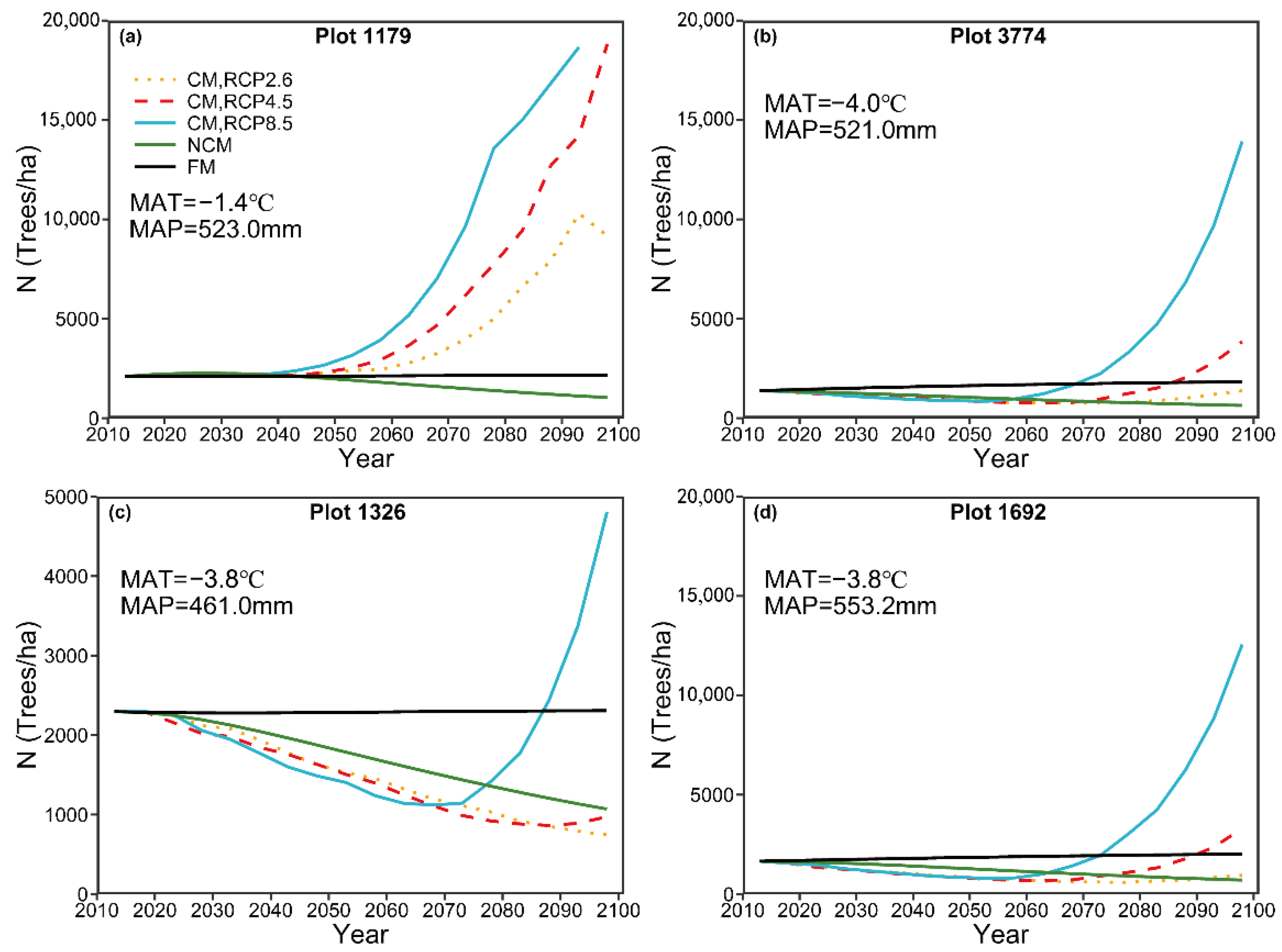
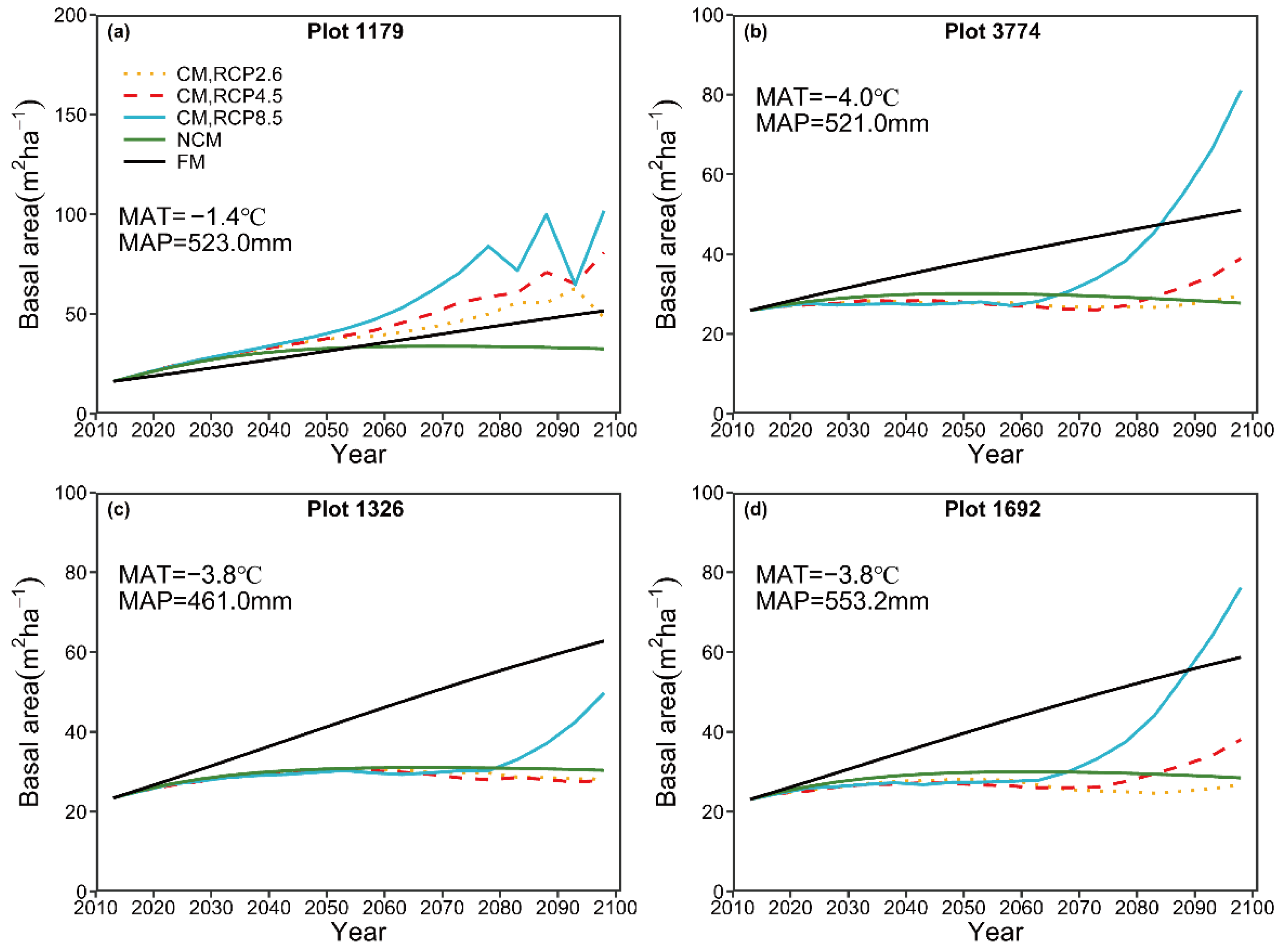
For prediction of 5-year intervals, the three models, i.e., FM, NCM, and CM, exhibited no pronounced differences in predictive performance for the focal species groups. We, therefore, recommended the FM, which has a simple structure and is easier to develop, to conduct short-term predictions. However, we found that the predicted long-term tree density and basal area by the FM showed a simple linear pattern, which may not be the true case (Figure 6 and Figure 7). Although NCM could generate more robust long-term predictions compared with FM, it might not be effective for long-term prediction because it neglected the long-term effects of climate variables on forest growth [58,64,65], recruitment [66,67,68], and mortality [64,69,70].

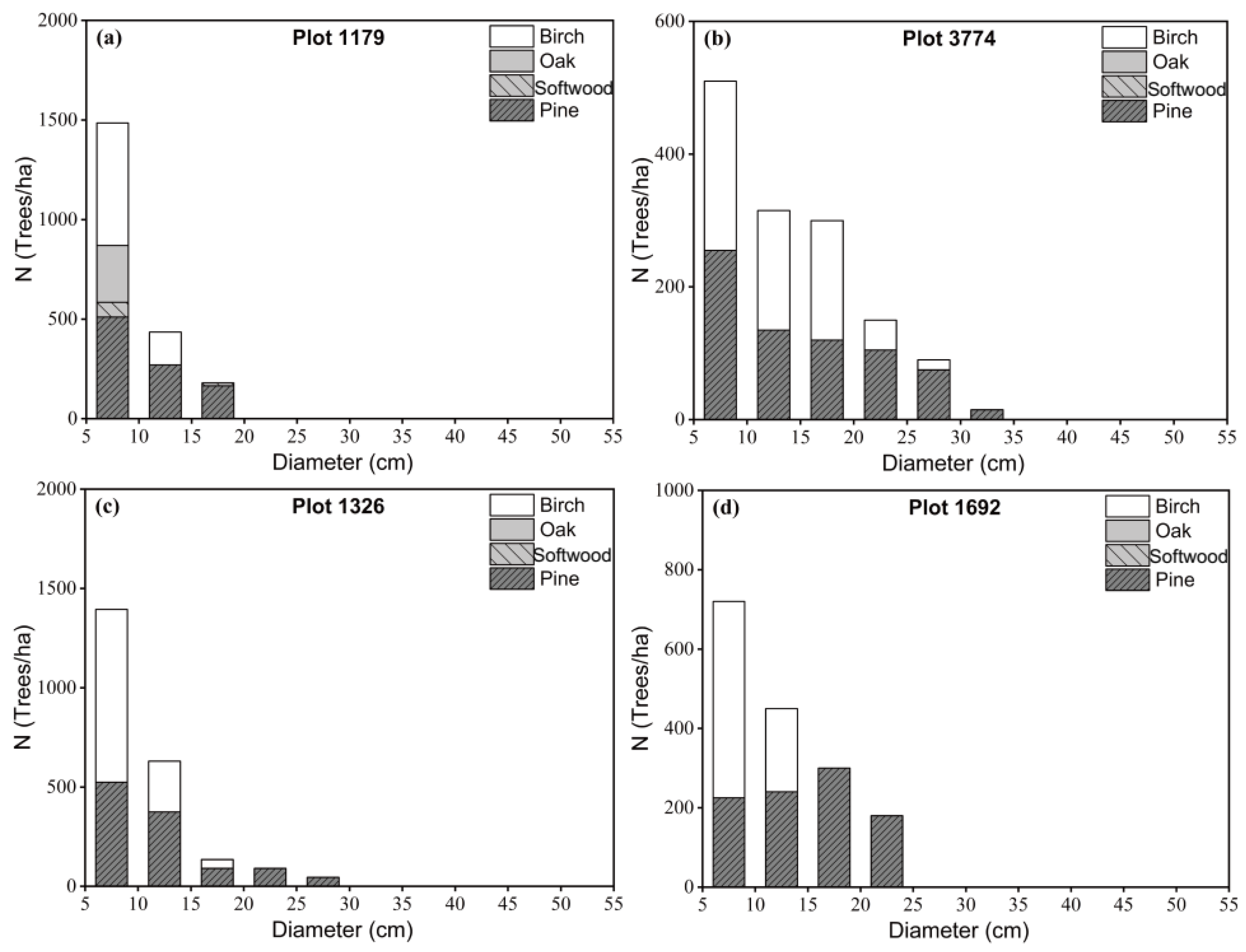
For long-term prediction, the predicted number of trees by the NCM suggests a decreasing trend, which could be explained by competition-induced self-thinning. The predicted basal area by the NCM showed a slightly increasing pattern and then reached a steady condition. The predicted patterns for the number of trees and basal area are in general consistent with the pattern in natural forest succession reported by Liang [44]. By contrast, the predicted number of trees by the CM under three different climate change scenarios, in general, indicated a pronounced increasing pattern, though plot 1326 showed a decreasing pattern before 2070 (Figure 6). A similar increasing pattern was also detected for the basal area under the three different RCPs (Figure 7). Similar results have been documented by many authors [14,71]. For example, Ruiz-Benito, Madrigal-Gonzalez, Ratcliffe, Coomes, Kändler, Lehtonen, Wirth and Zavala [71] reported that climatic warming caused an increase in stand average basal area, though this increase was offset by water availability. The predicted change in the steady state of natural stands suggests that increases in emissions can result in significant increases in stand density and basal area, which could preclude a steady state. Increases in stand density might reduce the economic value of forests and result in natural disasters, such as snow break, windthrow, and forest canopy fires. For example, high stand density can result in a large slenderness coefficient, which might increase the probability of windthrow or snow break [72,73]. Therefore, silvicultural practices should be implemented to mitigate the deleterious effects of climate change. For example, intermediate thinning intervals could be reduced or thinning intensity might be increased to manipulate stand density so that forests would be resistant to windthrow, snow break, or canopy fire.

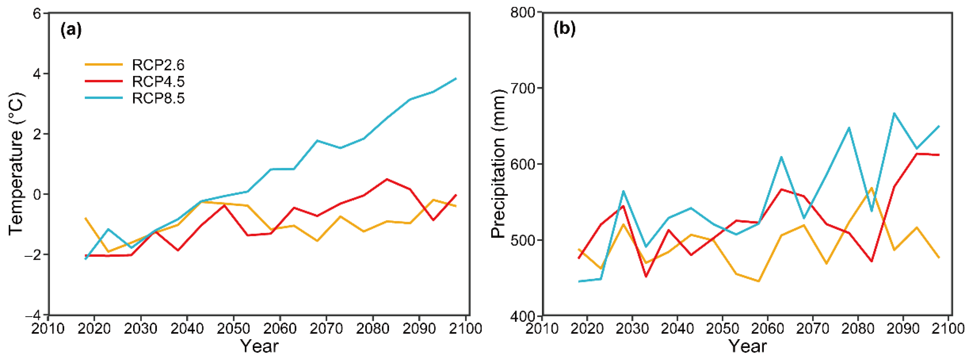
Fast-growing short-rotation trees accumulate more carbon in the leaves, stems, and roots and thus have higher net annual carbon sequestration rates than slow-growing trees. However, forests with slow-growing long-rotation trees have larger carbon stocks over the long term. Kaul, et al. [74] estimated the carbon sequestration potential of slow-growing sal (Shorea robusta Gaertn. f.), fast-growing Eucalyptus (Eucalyptus tereticornis Sm.), fast-growing poplar (Populus deltoides Marsh), and moderate-growing teak (Tectona grandis Linn. f.) forests in India and found that the living biomass of slow-growing long-rotation sal forests had the largest carbon stock; the opposite pattern was observed for net annual carbon sequestration rates. Sugden [75] showed that slow-growing trees sequester more carbon and argued that higher levels of carbon accumulation are achieved in communities of slow-growing species, indicating that slow-growing trees should be used for enrichment planting. The effects of increasing atmospheric CO₂ concentrations between the different GCMs (RCP2.6, RCP4.5, and RCP8.5) on MAT and MAP were similar to the patterns in emission intensity; for example, MAT under PRC 8.5 (high emission intensity) exhibited the sharpest increase, followed by RCP4.5 (intermediate emission intensity) and RCP2.6 (low peak-and-decay emission intensity) (Figure 3). This finding suggests that atmospheric CO₂ concentrations are positively correlated with MAT and MAP. The pattern of variation in the predicted number of trees, basal area, species diversity, and size diversity was similar to that in emissions, suggesting that emissions contributed to changes in these variables. For example, the sharpest increase in the predicted number of trees was observed under RCP8.5, followed by RCP4.5 and RCP2.6 (Figure 6).

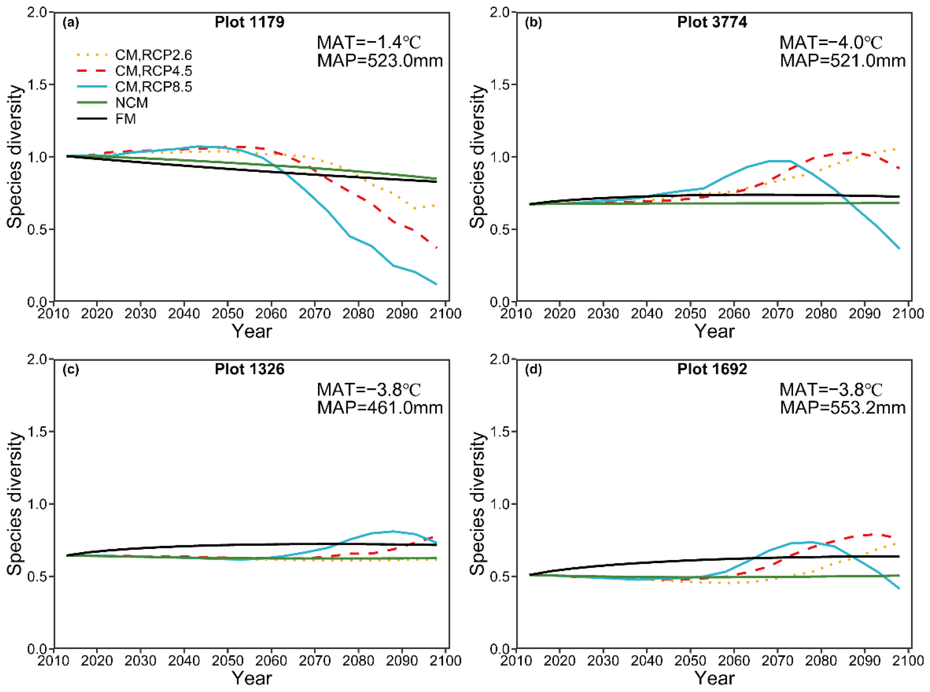
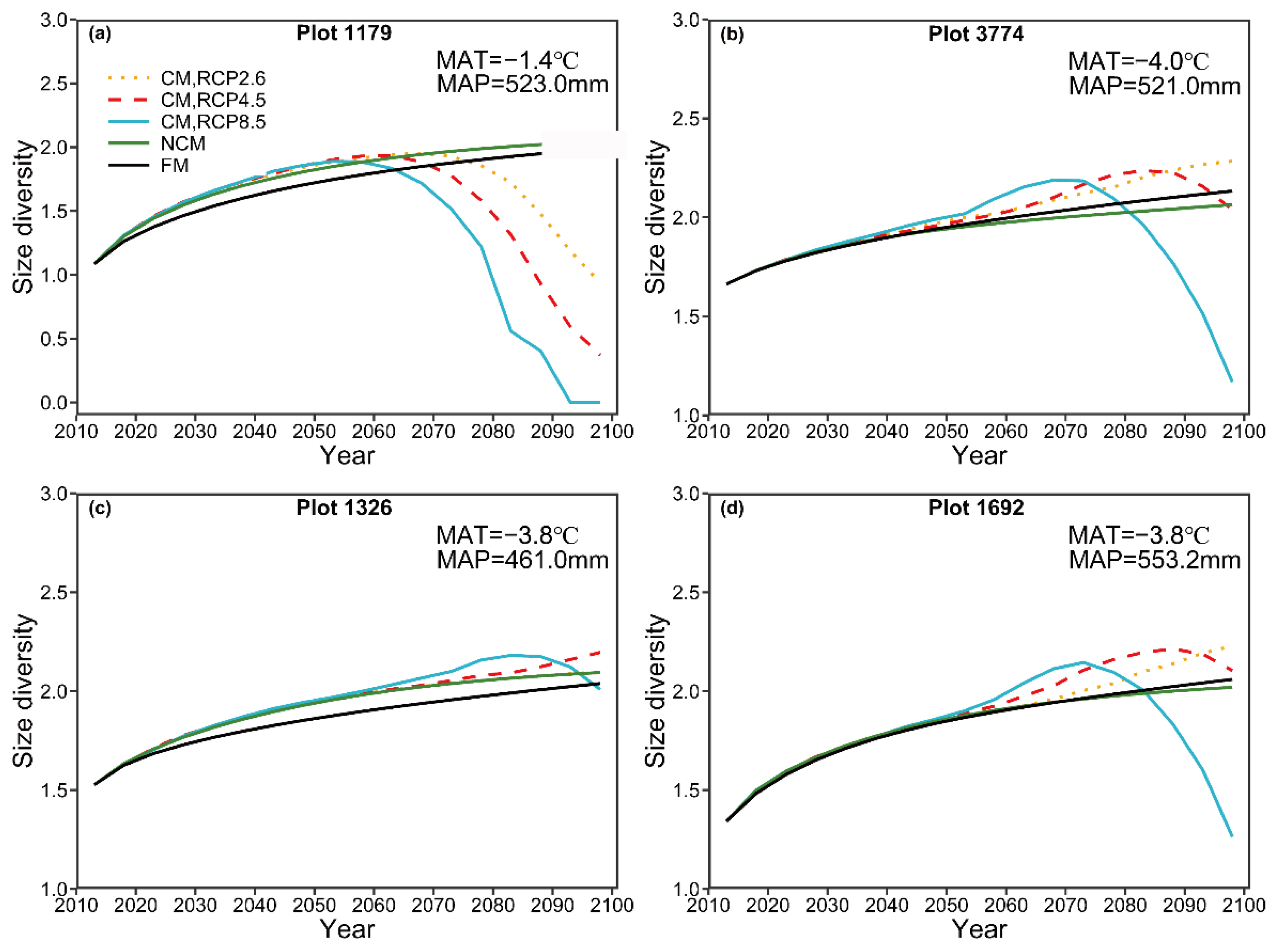
For long-term prediction, the predicted species diversity by the NCM, in general, showed almost no variation in time series, though a slightly decreasing trend was detected for plot 1179. By contrast, the species diversity predicted by the CM under these three climate change scenarios first shows an increasing pattern and then decreases, suggesting that species diversity could be negatively influenced by climate change. Many authors [76,77,78,79] have reported the results. For instance, Thuiller, et al. [80] projected late 21st-century distributions for 1350 European plants species under seven climate change scenarios and found that more than half of European plant species could be vulnerable or threatened by 2080. Moreover, we observed that the predicted patterns of species diversity shared similar tendencies as emissions. The long-term predicted size diversity by the CM under three RCPs shared the same trend with the predicted species diversity, indicating climate change (increasing CO₂) can reduce tree size diversity and the decreasing trend is dependent on emissions.

5. Conclusions

In this study, a climate-sensitive, transition-matrix growth model was developed to forecast the dynamics of Larix gmelinii mixed-species natural forests under different climate scenarios in China. For purpose of comparison, we also produced a conventional fixed-parameter transition matrix model, as well as a variable-transition model that did not consider climate change. No differences were observed among the three predictive models in their short-term prediction ability (5 years in this study). However, the long-term prediction ability of the CM under the three different RCPs was superior to that of the FM and NCM. The long-term predictions of the CM indicated that increases in emissions could lead to significant increases in stand density and basal area, which might result in natural disasters, such as snow break, windthrow, and forest fire. Silvicultural practices, such as reducing the intermediate thinning interval and the enrichment planting of slow-growing trees, should be implemented to mitigate the negative effects of climate change.

References

1. Yang, Z.; Zhou, G.; Yin, X.; Jia, B. Geographic distribution of Larix gmelinii natural forest in China and its climatic suitability. Chin. J. Ecol. 2014, 33, 1429. [Google Scholar]
2. Hu, H.; Hu, T.; Sun, L. Spatial heterogeneity of soil respiration in a Larix gmelinii forest and the response to prescribed fire in the Greater Xing′ an Mountains, China. J. For. Res. 2016, 27, 1153–1162. [Google Scholar] [CrossRef]
3. Liu, Y.; Yue, C.; Wei, X.; Blanco, J.A.; Trancoso, R. Tree profile equations are significantly improved when adding tree age and stocking degree: An example for Larix gmelinii in the Greater Khingan Mountains of Inner Mongolia, northeast China. Eur. J. For. Res. 2020, 139, 443–458. [Google Scholar] [CrossRef]
4. Administration, S.F. China Forest Resource Report (2014–2018); China Forestry Press: Beijing, China, 2019. [Google Scholar]
5. Barchenkov, A. Morphological variability and quality of seeds of Larix gmelinii (Rupr.) Rupr. Contemp. Probl. Ecol. 2011, 4, 327–333. [Google Scholar] [CrossRef]
6. Wang, C.; Gower, S.T.; Wang, Y.; Zhao, H.; Yan, P.; Bond-Lamberty, B.P. The influence of fire on carbon distribution and net primary production of boreal Larix gmelinii forests in north-eastern China. Glob. Change Biol. 2001, 7, 719–730. [Google Scholar] [CrossRef]
7. Zhou, H.; Ren, H.; Lu, J. Mechanical properties of Chinese larch (Larix gmelinii) dimension lumber. For. Prod. J. 2016, 66, 119–125. [Google Scholar] [CrossRef]
8. Ishiguri, F.; Iki, T.; Otsuka, K.; Takahashi, Y.; Nezu, I.; Tumenjargal, B.; Ohshima, J.; Yokota, S. Wood and lumber properties of Larix gmelinii var. olgensis planted in Japan. BioResources 2019, 14, 8072–8081. [Google Scholar]
9. Zhang, P.; Shao, G.; Zhao, G.; Le Master, D.C.; Parker, G.R.; Dunning, J.B., Jr.; Li, Q. China’s forest policy for the 21st century. Science 2000, 288, 2135–2136. [Google Scholar] [CrossRef] [PubMed] [Green Version]
10. Yu, D.; Zhou, L.; Zhou, W.; Ding, H.; Wang, Q.; Wang, Y.; Wu, X.; Dai, L. Forest Management in Northeast China: History, Problems, and Challenges. Env. Manag. 2011, 48, 1122–1135. [Google Scholar] [CrossRef] [PubMed]
11. Hua, F.; Xu, J.; Wilcove, D.S. A new opportunity to recover native forests in China. Conserv. Lett. 2018, 11, e12396. [Google Scholar] [CrossRef] [Green Version]
12. Yang, H. China’s natural forest protection program: Progress and impacts. For. Chron. 2017, 93, 113–117. [Google Scholar] [CrossRef] [Green Version]
13. Wang, W.; Bai, Y.; Jiang, C.; Yang, H.; Meng, J. Development of a linear mixed-effects individual-tree basal area increment model for masson pine in Hunan Province, South-central China. J. Sustain. For. 2019, 39, 526–541. [Google Scholar] [CrossRef]
14. Du, X.; Chen, X.; Zeng, W.; Meng, J. A climate-sensitive transition matrix growth model for uneven-aged mixed-species oak forests in North China. For. Int. J. For. Res. 2020, 94, 258–277. [Google Scholar] [CrossRef]
15. Sterba, H. Equilibrium curves and growth models to deal with forests in transition to uneven-aged structure-application in two sample stands. Silva Fenn. 2004, 38, 413–423. [Google Scholar] [CrossRef] [Green Version]
16. Lars, D.; Urban, N.; Lars, L. Simulated transformation of even-aged Norway spruce stands to multi-layered forests: An experiment to explore the potential of tree size differentiation. Forestry 2014, 87, 239–248. [Google Scholar]
17. Weiskittel, A.R.; Hann, D.W.; Kershaw Jr, J.A.; Vanclay, J.K. Forest Growth and Yield Modeling; John Wiley & Sons: Hoboken, NJ, USA, 2011. [Google Scholar]
18. Liang, J.; Picard, N. Matrix model of forest dynamics: An overview and outlook. For. Sci. 2013, 59, 359–378. [Google Scholar] [CrossRef]
19. Peng, C. Growth and yield models for uneven-aged stands: Past, present and future. For. Ecol. Manag. 2000, 132, 259–279. [Google Scholar] [CrossRef]
20. DeAngelis, D.; Rose, K. Which individual-based approach is most appropriate for a given problem. Individ. -Based Models Approaches Ecol. Popul. Communities Ecosyst. 1992, 8, 67–87. [Google Scholar]
21. Hao, Z.; Zhang, J.; Song, B.; Ye, J.; Li, B. Vertical structure and spatial associations of dominant tree species in an old-growth temperate forest. For. Ecol. Manag. 2007, 252, 1–11. [Google Scholar] [CrossRef]
22. Pan, Y.; Birdsey, R.A.; Fang, J.; Houghton, R.; Kauppi, P.E.; Kurz, W.A.; Phillips, O.L.; Shvidenko, A.; Lewis, S.L.; Canadell, J.G. A large and persistent carbon sink in the world’s forests. Science 2011, 333, 988–993. [Google Scholar] [CrossRef] [PubMed] [Green Version]
23. Bellassen, V.; Luyssaert, S. Carbon sequestration: Managing forests in uncertain times. Nat. News 2014, 506, 153. [Google Scholar] [CrossRef] [PubMed] [Green Version]
24. Swank, W.T.; Vose, J.M.; McNulty, S.G. Potential climate change effects on loblolly pine forest productivity and drainage across the southern United States. AMBIO—A J. Hum. Environ. 1996, 25, 449–453. [Google Scholar]
25. Lucash, M.S.; Scheller, R.M.; Kretchun, A.M.; Clark, K.L.; Hom, J. Impacts of fire and climate change on long-term nitrogen availability and forest productivity in the New Jersey Pine Barrens. Can. J. For. Res. 2014, 44, 404–412. [Google Scholar] [CrossRef] [Green Version]
26. Allen, C.D.; Macalady, A.K.; Chenchouni, H.; Bachelet, D.; Mcdowell, N.; Vennetier, M.; Kitzberger, T.; Rigling, A.; Breshears, D.D.; Hogg, E.H. A global overview of drought and heat-induced tree mortality reveals emerging climate change risks for forests. For.Ecol.Manag. 2010, 259, 660–684. [Google Scholar] [CrossRef] [Green Version]
27. Luo, Y.; Chen, H. Observations from old forests underestimate climate change effects on tree mortality. Nat. Commun. 2013, 4, 1665. [Google Scholar] [CrossRef] [PubMed]
28. Zhang, X.; Lei, Y.; Yong, P.; Liu, X.; Wang, J. Tree mortality in response to climate change induced drought across Beijing, China. Clim. Change 2014, 124, 179–190. [Google Scholar] [CrossRef]
29. Brodie, J.; Post, E.; Watson, F.; Berger, J. Climate change intensification of herbivore impacts on tree recruitment. Proc. R. Soc. B Biol. Sci. 2012, 279, 1366–1370. [Google Scholar] [CrossRef] [PubMed] [Green Version]
30. Peltier, D.; Ibez, I. Patterns and Variability in Seedling Carbon Assimilation: Implications for Tree Recruitment Under Climate Change. In Proceedings of the 99th ESA Annual Convention 2014, Sacramento, CA, USA, 10–15 August 2014. [Google Scholar]
31. Boden, S.; Pyttel, P.; Eastaugh, C. Impacts of climate change on the establishment, distribution, growth and mortality of Swiss stone pine (Pinus cembra L.). Iforest-Biogeosci. For. 2010, 3, 82. [Google Scholar] [CrossRef]
32. Eastaugh, C.S.; Pötzelsberger, E.; Hasenauer, H. Assessing the impacts of climate change and nitrogen deposition on Norway spruce (Picea abies L. Karst) growth in Austria with BIOME-BGC. Tree Physiol. 2011, 31, 262–274. [Google Scholar] [CrossRef] [Green Version]
33. Lei, X.; Yu, L.; Hong, L. Climate-sensitive integrated stand growth model (CS-ISGM) of Changbai larch (Larix olgensis) plantations. For. Ecol. Manag. 2016, 376, 265–275. [Google Scholar] [CrossRef]
34. Dănescu, A.; Albrecht, A.T.; Bauhus, J.; Kohnle, U. Geocentric alternatives to site index for modeling tree increment in uneven-aged mixed stands. For. Ecol. Manag. 2017, 392, 1–12. [Google Scholar] [CrossRef]
35. Wang, T.; Wang, G.; Innes, J.L.; Seely, B.; Chen, B. ClimateAP: An application for dynamic local downscaling of historical and future climate data in Asia Pacific. Front. Agric. Sci. Eng. 2017, 4, 448–458. [Google Scholar] [CrossRef] [Green Version]
36. Swart, N.C.; Cole, J.N.; Kharin, V.V.; Lazare, M.; Scinocca, J.F.; Gillett, N.P.; Anstey, J.; Arora, V.; Christian, J.R.; Hanna, S. The Canadian earth system model version 5 (CanESM5. 0.3). Geosci. Model Dev. 2019, 12, 4823–4873. [Google Scholar] [CrossRef] [Green Version]
37. Gebrechorkos, S.H.; Hülsmann, S.; Bernhofer, C. Regional climate projections for impact assessment studies in East Africa. Environ. Res. Lett. 2019, 14, 044031. [Google Scholar] [CrossRef]
38. Taylor, K.E.; Stouffer, R.J.; Meehl, G.A. An overview of CMIP5 and the experiment design. Bull. Am. Meteorol. Soc. 2012, 93, 485–498. [Google Scholar] [CrossRef] [Green Version]
39. Van Vuuren, D.P.; Edmonds, J.A.; Kainuma, M.; Riahi, K.; Weyant, J. A special issue on the RCPs. Clim. Change 2011, 109, 1–5. [Google Scholar] [CrossRef] [Green Version]
40. Stage, A.R. An expression for the effect of aspect, slope, and habitat type on tree growth. For. Sci. 1976, 22, 457–460. [Google Scholar]
41. Tobin, J. Estimation of relationships for limited dependent variables. Econom. J. Econom. Soc. 1958, 26, 24–36. [Google Scholar] [CrossRef] [Green Version]
42. Liang, J.; Zhou, M.; Verbyla, D.L.; Zhang, L.; Springsteen, A.L.; Malone, T. Mapping forest dynamics under climate change: A matrix model. For. Ecol. Manag. 2011, 262, 2250–2262. [Google Scholar] [CrossRef]
43. Mac Nally, R. Regression and model-building in conservation biology, biogeography and ecology: The distinction between–and reconciliation of–‘predictive’and ‘explanatory’models. Biodivers. Conserv. 2000, 9, 655–671. [Google Scholar] [CrossRef]
44. Liang, J. Dynamics and management of Alaska boreal forest: An all-aged multi-species matrix growth model. For. Ecol. Manag. 2010, 260, 491–501. [Google Scholar] [CrossRef]
45. Lin, C.-R.; Buongiorno, J. Fixed versus variable-parameter matrix models of forest growth: The case of maple-birch forests. Ecol. Model. 1997, 99, 263–274. [Google Scholar] [CrossRef]
46. Team, R.C. R: A Language and Environment for Statistical Computing; R Foundation for Statistical Computing: Vienna, Austria, 2010. [Google Scholar]
47. Pedro, M.S.; Rammer, W.; Seidl, R. A disturbance-induced increase in tree species diversity facilitates forest productivity. Landsc. Ecol. 2016, 31, 989–1004. [Google Scholar] [CrossRef]
48. Fichtner, A.; Härdtle, W.; Li, Y.; Bruelheide, H.; Kunz, M.; von Oheimb, G. From competition to facilitation: How tree species respond to neighbourhood diversity. Ecol. Lett. 2017, 20, 892–900. [Google Scholar] [CrossRef] [PubMed]
49. Aussenac, R.; Bergeron, Y.; Gravel, D.; Drobyshev, I. Interactions among trees: A key element in the stabilising effect of species diversity on forest growth. Funct. Ecol. 2019, 33, 360–367. [Google Scholar] [CrossRef]
50. Sapijanskas, J.; Paquette, A.; Potvin, C.; Kunert, N.; Loreau, M. Tropical tree diversity enhances light capture through crown plasticity and spatial and temporal niche differences. Ecology 2014, 95, 2479–2492. [Google Scholar] [CrossRef]
51. Hisano, M.; Chen, H.Y.; Searle, E.B.; Reich, P.B. Species-rich boreal forests grew more and suffered less mortality than species-poor forests under the environmental change of the past half-century. Ecol. Lett. 2019, 22, 999–1008. [Google Scholar] [CrossRef] [PubMed]
52. Wang, W.; Lei, X.; Ma, Z.; Kneeshaw, D.D.; Peng, C. Positive relationship between aboveground carbon stocks and structural diversity in spruce-dominated forest stands in New Brunswick, Canada. For. Sci. 2011, 57, 506–515. [Google Scholar]
53. Dănescu, A.; Albrecht, A.T.; Bauhus, J. Structural diversity promotes productivity of mixed, uneven-aged forests in southwestern Germany. Oecologia 2016, 182, 319–333. [Google Scholar] [CrossRef]
54. Ali, A.; Yan, E.-R.; Chen, H.Y.; Chang, S.X.; Zhao, Y.-T.; Yang, X.-D.; Xu, M.-S. Stand structural diversity rather than species diversity enhances aboveground carbon storage in secondary subtropical forests in Eastern China. Biogeosciences 2016, 13, 4627–4635. [Google Scholar] [CrossRef] [Green Version]
55. Ercanli, İ. Positive effect of forest structural diversity on aboveground stand carbon stocks for even-aged Scots pine (Pinus sylvestris L.) stands in the Sarıçiçek Forest, Northern Turkey. Scand. J. For. Res. 2018, 33, 455–463. [Google Scholar] [CrossRef]
56. Ruan, L.-p.; Lu, Y.-c.; Meng, J.-h. Plantation transformation alternatives determine carbon sequestration capacity—a case study with Pinus massoniana in southern China. J. Mt. Sci. 2020, 17, 919–930. [Google Scholar] [CrossRef]
57. Raich, J.W.; Russell, A.E.; Kitayama, K.; Parton, W.J.; Vitousek, P.M. Temperature influences carbon accumulation in moist tropical forests. Ecology 2006, 87, 76–87. [Google Scholar] [CrossRef] [PubMed] [Green Version]
58. Toledo, M.; Poorter, L.; Peña-Claros, M.; Alarcón, A.; Balcázar, J.; Leaño, C.; Licona, J.C.; Llanque, O.; Vroomans, V.; Zuidema, P. Climate is a stronger driver of tree and forest growth rates than soil and disturbance. J. Ecol. 2011, 99, 254–264. [Google Scholar] [CrossRef]
59. Laubhann, D.; Sterba, H.; Reinds, G.J.; De Vries, W. The impact of atmospheric deposition and climate on forest growth in European monitoring plots: An individual tree growth model. For. Ecol. Manag. 2009, 258, 1751–1761. [Google Scholar] [CrossRef]
60. Schuur, E.A. Productivity and global climate revisited: The sensitivity of tropical forest growth to precipitation. Ecology 2003, 84, 1165–1170. [Google Scholar] [CrossRef]
61. Mann, D.H.; Rupp, T.S.; Olson, M.A.; Duffy, P.A. Is Alaska’s boreal forest now crossing a major ecological threshold? Arct. Antarct. Alp. Res. 2012, 44, 319–331. [Google Scholar] [CrossRef] [Green Version]
62. Barber, V.A.; Juday, G.P.; Finney, B.P. Reduced growth of Alaskan white spruce in the twentieth century from temperature-induced drought stress. Nature 2000, 405, 668–673. [Google Scholar] [CrossRef]
63. Williams, A.P.; Allen, C.D.; Macalady, A.K.; Griffin, D.; Woodhouse, C.A.; Meko, D.M.; Swetnam, T.W.; Rauscher, S.A.; Seager, R.; Grissino-Mayer, H.D. Temperature as a potent driver of regional forest drought stress and tree mortality. Nat. Clim. Change 2013, 3, 292–297. [Google Scholar] [CrossRef]
64. Battles, J.J.; Robards, T.; Das, A.; Waring, K.; Gilless, J.K.; Biging, G.; Schurr, F. Climate change impacts on forest growth and tree mortality: A data-driven modeling study in the mixed-conifer forest of the Sierra Nevada, California. Clim. Change 2008, 87, 193–213. [Google Scholar] [CrossRef]
65. Hartl-Meier, C.; Dittmar, C.; Zang, C.; Rothe, A. Mountain forest growth response to climate change in the Northern Limestone Alps. Trees 2014, 28, 819–829. [Google Scholar] [CrossRef]
66. Matías, L.; Jump, A.S. Impacts of predicted climate change on recruitment at the geographical limits of Scots pine. J. Exp. Bot. 2014, 65, 299–310. [Google Scholar] [CrossRef] [Green Version]
67. Mueter, F.J.; Bond, N.A.; Ianelli, J.N.; Hollowed, A.B. Expected declines in recruitment of walleye pollock (Theragra chalcogramma) in the eastern Bering Sea under future climate change. ICES J. Mar. Sci. 2011, 68, 1284–1296. [Google Scholar] [CrossRef] [Green Version]
68. Ibáñez, I.; Clark, J.S.; LaDeau, S.; Lambers, J.H.R. Exploiting temporal variability to understand tree recruitment response to climate change. Ecol. Monogr. 2007, 77, 163–177. [Google Scholar] [CrossRef]
69. Hartmann, H.; Bastos, A.; Das, A.J.; Esquivel-Muelbert, A.; Hammond, W.M.; Martínez-Vilalta, J.; McDowell, N.G.; Powers, J.S.; Pugh, T.A.; Ruthrof, K.X. Climate Change Risks to Global Forest Health: Emergence of Unexpected Events of Elevated Tree Mortality Worldwide. Annu. Rev. Plant Biol. 2022, 73, 1. [Google Scholar] [CrossRef]
70. Klein, T.; Cahanovitc, R.; Sprintsin, M.; Herr, N.; Schiller, G. A nation-wide analysis of tree mortality under climate change: Forest loss and its causes in Israel 1948–2017. For. Ecol. Manag. 2019, 432, 840–849. [Google Scholar] [CrossRef]
71. Ruiz-Benito, P.; Madrigal-Gonzalez, J.; Ratcliffe, S.; Coomes, D.A.; Kändler, G.; Lehtonen, A.; Wirth, C.; Zavala, M.A. Stand structure and recent climate change constrain stand basal area change in European forests: A comparison across boreal, temperate, and Mediterranean biomes. Ecosystems 2014, 17, 1439–1454. [Google Scholar] [CrossRef]
72. Meng, J.; Bai, Y.; Zeng, W.; Ma, W. A management tool for reducing the potential risk of windthrow for coastal Casuarina equisetifolia L. stands on Hainan Island, China. Eur. J. For. Res. 2017, 136, 543–554. [Google Scholar] [CrossRef]
73. Del Río, M.; Pretzsch, H.; Bončina, A.; Avdagić, A.; Bielak, K.; Binder, F.; Coll, L.; Hilmers, T.; Höhn, M.; Kašanin-Grubin, M. Assessment of indicators for climate smart management in mountain forests. Clim. -Smart For. Mt. Reg. 2021, 40, 59. [Google Scholar]
74. Kaul, M.; Mohren, G.; Dadhwal, V. Carbon storage and sequestration potential of selected tree species in India. Mitig. Adapt. Strateg. Glob. Change 2010, 15, 489–510. [Google Scholar] [CrossRef] [Green Version]
75. Sugden, A.M. Slow-growing trees sequester more carbon. Science 2019, 364, 1248–1249. [Google Scholar]
76. Li, R.; Xu, M.; Wong, M.H.G.; Qiu, S.; Sheng, Q.; Li, X.; Song, Z. Climate change-induced decline in bamboo habitats and species diversity: Implications for giant panda conservation. Divers. Distrib. 2015, 21, 379–391. [Google Scholar] [CrossRef]
77. Murphy, D.D.; Weiss, S.B. Effects of climate change on biological diversity in western North America: Species losses and mechanisms. In Global Warming and Biological Diversity; Yale University Press: New Haven, CT, USA, 1992; pp. 355–368. [Google Scholar]
78. Lafferty, K.D. The ecology of climate change and infectious diseases. Ecology 2009, 90, 888–900. [Google Scholar] [CrossRef] [PubMed]
79. Muhlfeld, C.C.; Kovach, R.P.; Jones, L.A.; Al-Chokhachy, R.; Boyer, M.C.; Leary, R.F.; Lowe, W.H.; Luikart, G.; Allendorf, F.W. Invasive hybridization in a threatened species is accelerated by climate change. Nat. Clim. Change 2014, 4, 620–624. [Google Scholar] [CrossRef]
80. Thuiller, W.; Lavorel, S.; Araújo, M.B.; Sykes, M.T.; Prentice, I.C. Climate change threats to plant diversity in Europe. Proc. Natl. Acad. Sci. USA 2005, 102, 8245–8250. [Google Scholar] [CrossRef] [PubMed] [Green Version]
Figure 1. Distribution of the sample plots for oaks in the studied area.
Forests 13 00574 g001
Figure 2. Mean annual temperature (a) and mean annual precipitation (b) in the state-owned forest region of the Greater Khingan Mountains.
Forests 13 00574 g002
Figure 3. Temporal changes of MAT (°C; panel a) and MAP (mm; panel b) under three RCPs.
Forests 13 00574 g003
Figure 4. Diameter distribution of NFI plot numbers 1179, 3774, 1326, and 1692 by species group and diameter class.
Forests 13 00574 g004
Figure 5. Average predicted and observed (with 95 % confidence intervals) basal area by diameter class and species group using the cross-validation technique, based on the first inventory of 428 sample plots.
Forests 13 00574 g005
Figure 6. Long-term prediction of tree numbers by the climate-sensitive model (CM) under 3 different RCPs, the variable transition model which did not expect climate change (NCM), and the fixed-parameter model (FM), using NFI plot numbers 1179, 3774, 1326, and 1692. The value of the MAT is the mean annual temperature between 2013 and 2018 and MAP represents the mean annual precipitation of the same period.
Forests 13 00574 g006
Figure 7. Long-term prediction of the basal area by the climate-sensitive model (CM) under three RCPs, the variable transition model which did not expect climate change (NCM), and the fixed-parameter model (FM), using NFI plots 1179, 3774, 1326, and 1692. The value of the MAT is the mean annual temperature between 2013 and 2018 and MAP represents the mean annual precipitation of the same period.
Forests 13 00574 g007
Figure 8. Long-term prediction of species diversity by the climate-sensitive model (CM) under three RCPs, the variable transition model which did not expect climate change (NCM), and the fixed-parameter model (FM), using NFI plots 1179, 3774, 1326, and 1692. The value of the MAT is the mean annual temperature between 2013 and 2018 and MAP represents the mean annual precipitation of the same period.
Forests 13 00574 g008
Figure 9. Long-term prediction of size diversity by the climate-sensitive model (CM) under three RCPs, the variable transition model which did not expect climate change (NCM), and the fixed-parameter model (FM), using NFI plots 1179, 3774, 1326, and 1692. The value of the MAT is the mean annual temperature between 2013 and 2018 and MAP represents the mean annual precipitation of the same period.
Forests 13 00574 g009