Climate Change Effects on Height–Diameter Allometric Relationship Vary with Tree Species and Size for Larch Plantations in Northern and Northeastern China

Abstract

Tree height–diameter relationship is very important in forest investigation, describing forest structure and estimating carbon storage. Climate change may modify the relationship. However, our understanding of the effects of climate change on the height–diameter allometric relationship is still limited at large scales. In this study, we explored how climate change effects on the relationship varied with tree species and size for larch plantations in northern and northeastern China. Based on the repeated measurement data of 535 plots from the 6th to 8th national forest inventory of China, climate-sensitive tree height–diameter models of larch plantations in north and northeast China were developed using two-level nonlinear mixed effect (NLME) method. The final model was used to analyze the height–diameter relationship of different larch species under RCP2.6, RCP 4.5, and RCP8.5 climate change scenarios from 2010 to 2100. The adjusted coefficient of determination $R_{adj}^2$, mean absolute error (MAE) and root mean squared error (RMSE) of the NLME models for calibration data were 0.92, 0.76 m and 1.06 m, respectively. The inclusion of climate variables mean annual temperature (MAT) and Hargreaves climatic moisture deficit (CMD) with random effects was able to increase $R_{adj}^2$ by 19.5% and reduce the AIC (Akaike’s information criterion), MAE and RMSE by 22.2%, 44.5% and 41.8%, respectively. The climate sensitivity of larch species was ranked as L. gmelinii > the unidentified species group > L. principis > L. kaempferi > L. olgensis under RCP4.5, but L. gmelinii > L. principis > the unidentified species group > L. olgensis > L. kaempferi under RCP2.6 and RCP8.5. Large trees were more sensitive to climate change than small trees.

1. Introduction

Tree height–diameter (H–D) models are one of the most useful tools in forest management. Because tree height measurement is time-consuming, expensive and difficult in over-crowed and dense forests, a small number of trees are typically subsampled in practice to measure tree height, while D is measured precisely for all trees in a plot [1]. Thus, H–D models are often constructed to predict missing total height measurements for the rest of the trees. Numerous H–D models have been developed [2,3,4,5,6,7,8,9,10,11,12,13,14,15]. These models showed that the H–D relationship was context-dependent, and varied with genetic characteristics [8], stand age [16], site condition [6,7,15,17], competition status [5,6,7,13], silvicultural treatment [18,19] and climate [9,11,20,21].

Under the background of global change, the effects of climate change on forest growth are great concerns [22,23,24,25]. However, how climate change modifies H–D relationships has only recently been considered [9,11,21,26,27]. For example, Hulshof et al. [9] developed mixed-effects models to test H–D allometric differences due to climate and functional groups, and models showed that temperature, and some extent precipitation, in part-explained tree H–D allometric variation. Climate variables can significantly explain the variation of the H–D relationship, and adding climate variables can improve the prediction performance of the model in the context of climate change. Zhang et al. [11] developed the tree level NLME model to show that temperature was a key climate factor shaping height–diameter allometry of Chinese fir, and tree height increased with rising MAT. Fortin et al. [21] developed generalized H–D models of 44 tree species across France and found that the temperature effect was significant for 33 species and the precipitation effect was significant only for 7 species. They estimated that two-thirds of climate sensitive species were expected to be generally shorter under the RCP 2.6 scenario.

However, there were substantial variations in the direction and magnitude of climatic effects on H–D relationships. For example, Hulshof et al. [9] showed that the coefficient of MAT was negative but the model developed by Zhang et al. [11] showed MAT had positive effects on H–D allometry. Feldpausch et al. [28] found that annual precipitation coefficient of variation, dry season length, and mean annual air temperature were key drivers of variation in H–D allometry at the pantropical and region scales. Ng’andwe et al. [27] found that temperature negatively modulated H–D allometry of Pinus merkusii var. latteri and P. michoacana var. cornuta Martínez in Zambia. Furthermore, how these climatic effects differ among tree species and sizes are not well understood. The climate effects on H–D relationship are likely to have an impact on tree stability, height estimation, yield prediction and forest management decision, thus making it necessary to examine it under climate change.

Larch is an economically and ecologically important genus of tree species in China, especially in the northern and northeastern regions. The area and volume of larch forests amount to 6.50 and 6.77 percent of the total forest, respectively [29]. Both empirical and process-based models found that future climate change would affect stand growth, productivity, and biological rotation of larch plantations [10,30,31,32,33], but how climate change will modify the H–D relationship is unknown yet. Therefore, the objectives of the study were: (1) to develop a climate-sensitive H–D model for larch plantations in north and northeast China; (2) to examine how the effects of future climate change on H–D relationship vary with larch species and tree sizes. Quantifying the effects of climate change will help better understand the H–D allometric relationship and adaptive forest management under climate change.

2. Materials and Methods

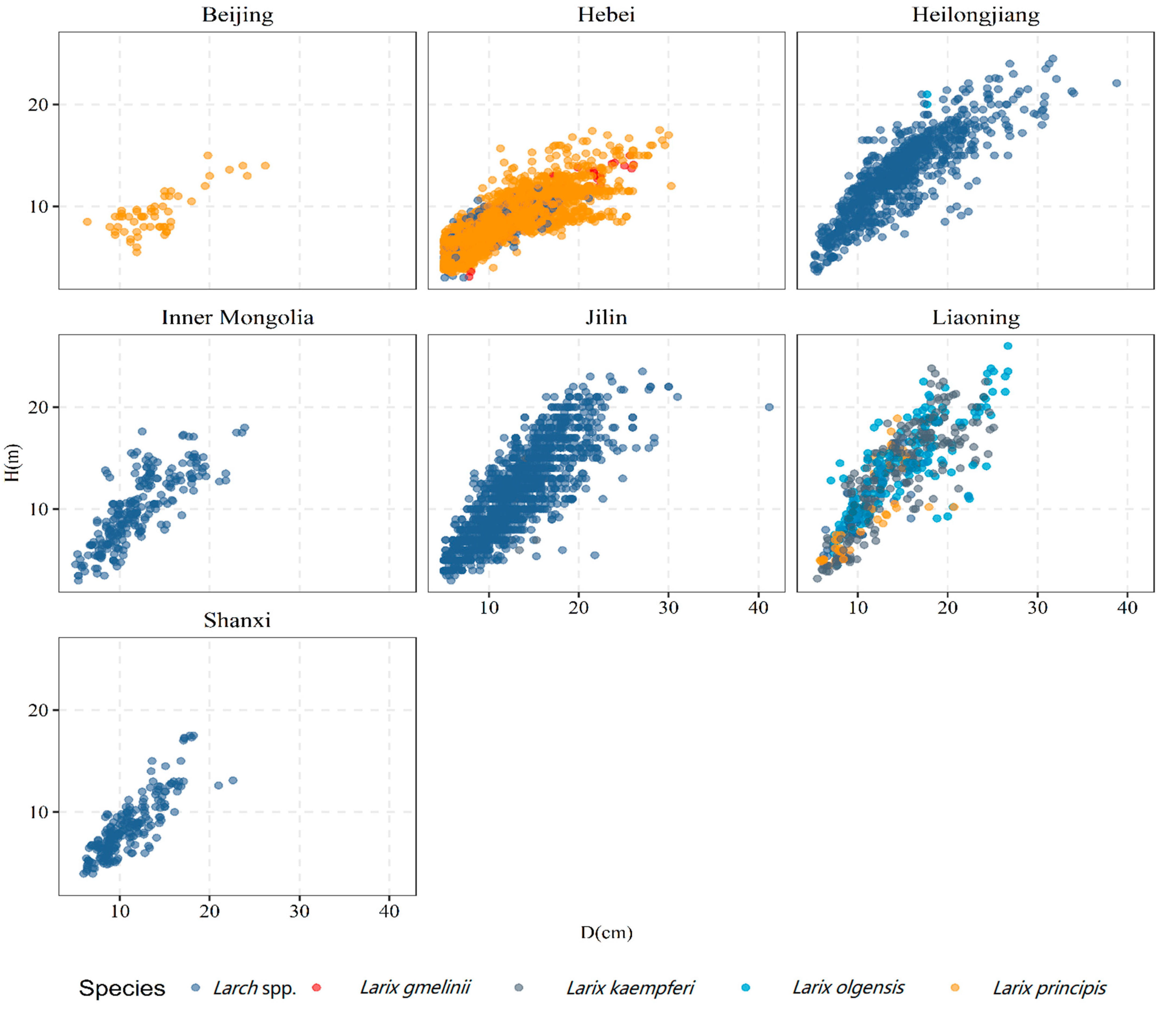
2.1. Tree Height–Diameter Data

Tree H–D data used in this study were from 6th (year 2000), 7th (year 2005) and 8th (year 2010) National Forest Inventories in 7 provinces (Beijing, Hebei, Shanxi, Liaoning, Jilin, Heilongjiang, and Inner Mongolia) in north and northeast China. We selected only pure larch plantation plots to develop the H–D model. The larch species presented in these plots are L. gmelinii, L. olgensis, L. kaempferi, L. principis. In addition, there were trees not identified to specific species which were recorded as larch. According to the protocol of NFI, heights of 3–5 average trees were measured in each plot. In total, 7304 pairs of H–D measurements in 535 plots were obtained across seven Provinces. Data were split into two parts for model calibration and validation by the following method: each plot was randomly allocated to a number between 1 and 535, and plots with number less than 20th percentile of all plots were assigned as validation data (1609 pairs in 107 plots) and the rest were fitting data (5695 pairs of H–D measurements in 428 plots).

Table 1. Summary statistics for tree and stand variables by provinces.

Data	Province	Number of Plots	Number of Tree Observations	D (cm)	H (m)	AGE (a)	N (Trees × ha−1)	BA (m2 × ha−1)
Calibration	Beijing	7	37	14.7 (4.6)	9.3 (2.3)	32.9 (10.6)	561.9 (418.5)	9.1 (9.9)
	Hebei	72	3326	10.7 (4.5)	7.9 (2.2)	21.7 (6.7)	1072.6 (540.9)	9.3 (7.3)
	Heilongjiang	96	706	14.5 (5.3)	13 (3.9)	27.9 (9.7)	653.9 (520.5)	4.6 (4.6)
	Jilin	132	1058	12.9 (4.7)	11.4 (4.4)	25.2 (9.9)	1032.2 (565.3)	9.0 (5.6)
	Liaoning	52	406	14.4 (4.8)	13.5 (4.5)	23.6 (10.2)	1292.3 (631.7)	13.5 (8.6)
	Inner Mongolia	35	188	12.2 (3.7)	10.1 (3.2)	25.8 (7.1)	855.1 (617.7)	8.0 (6.4)
	Shanxi	34	195	11.1 (3.1)	8.7 (2.8)	26.5 (9.3)	1297.8 (627.3)	9.4 (7.7)
	total	428	5916	11.9 (4.8)	9.6 (3.8)	23.6 (8.5)	977.2 (610.6)	8.5 (6.9)
Validation	Beijing	3	18	12.6 (1.7)	9.2 (1.6)	25.8 (3.1)	816.8 (469.2)	11.5 (10.7)
	Hebei	12	620	11.4 (3.8)	8.9 (2.3)	24.8 (7.6)	994.9 (607.2)	8.5 (5.4)
	Heilongjiang	27	193	15.2 (5.0)	13.1 (3.8)	29.5 (9.8)	559.3 (548.7)	6.0 (6.3)
	Jilin	38	351	13.5 (4.4)	11.9 (4.0)	28.4 (11.1)	904.2 (532.9)	8.2 (4.9)
	Liaoning	12	97	12.2 (4.5)	11.3 (5.4)	23.2 (9.3)	1207.8 (651.1)	17.7 (7.0)
	Inner Mongolia	11	53	11.1 (4.4)	9.1 (4.1)	28 (9.9)	1135.5 (835.4)	7.3 (6.4)
	Shanxi	4	21	9 (1.8)	6.7 (2.0)	17.9 (4.2)	848.6 (622.8)	7.3 (6.3)
	total	107	1353	12.5 (4.4)	10.4 (3.8)	26.3 (9.4)	902.6 (626.8)	8.6 (6.8)

Note: D, diameter at breast height; H, tree height; N, the number of trees per hectare; BA, basal area per hectare; AGE, stand average age; the numbers within parentheses are the standard deviation.

showed the summary statistics of tree and stand variables. The scatter plot can be found in Figure 1.

2.2. Climate Data

The current climatic data for model calibration were downloaded from ClimateAP, which is an application for dynamic local downscaling of historical and future climate data in Asia Pacific [34]. Seasonal and annual climate variables (averaged from 1980 to 2010) for a plot were produced based on latitude, longitude, and elevation (

Table 2. Descriptions of the candidate climatic variables.

Variable	Description
AHM	Annual heat:moisture index
CMD	Hargreaves climatic moisture deficit
DD_0	Degree-days below 0 °C
DD_18	Degree-days below 18 °C
DD18	Degree-days above 18 °C
DD5	Degree-days above 5 °C
EMT/°C	Extreme minimum temperature over a 30-year period
EXT/°C	Extreme maximum temperature over a 30-year period
EREF	Hargreaves reference evaporation
MAP/mm	Mean annual precipitation
MAT/°C	Mean annual temperature
MCMT/°C	Mean coldest month temperature
MWMT/°C	Mean warmest month temperature
NFFD	The number of frost-free days
PAS/mm	Precipitation as snow between August in previous year and July in current year
TD/°C	Temperature difference between MWMT and MCMT, or continentality

).

For projections of future H–D relationship under expected climate change, we used the latest climate change scenarios of the 5th Assessment Report from the IPCC using a downscaled global climate model (GCM) applied in three representative concentration pathways (RCPs), RCP2.6, RCP4.5, and RCP8.5 [35]. These pathways represent the scenarios with low, medium and high concentrations of greenhouse gases and predictive radiative forcing. The GCM model for future climate scenarios used in the study was CNRM-CM5 (The Centre National de Recherches Météorologiques coupled global climate Model) [36]. Future climate data for the time periods 2025 (average for 2010–2040), 2055 (average for 2040–2070) and 2085 (average for 2070–2100) were also downloaded from the ClimateAP.

2.3. Selection of Climate Variables

Principal Component Analysis (PCA) [37] can be an exploratory method for the evaluation of the climatic variability and robust as an auxiliary technique when used in combination with other statistical techniques [38]. We first used PCA method to analyze the data for all climate variables. Owing to climate variables with different units, all variables were standardized prior to PCA. Components explaining more than 80% of the variance were retained. For each component, variables with large loadings were selected for further analysis. These variables with strong correlations with H and the least multicollinearity among them were served as options for modelling.

2.4. Basic H–D Models

The basic H–D model was from Zang et al. [10] for the same tree species in the region and modified as Equation (1) which was a generalized H–D model with the inclusion of competition effects besides tree diameter.

$$H=1.3+\left(a_0+a_{1}BAL\right)\times {\left(1-\mathit{exp}\left(-\left(b_0+b_{1}BAL\right)\times D\right)\right)}^c+\epsilon$$

(1)

where $H$ is the total tree height (m), $D$ is the diameter at breast height (cm), BAL is the sum of the basal area of the trees larger than a subject tree, $a_0$,$a_1$, $b_0$, $b_1$ and $c$ are model parameters, which have their own biological characteristics, and $\epsilon$ is random error.

To evaluate the differences in H–D allometry among larch species, dummy variables S_m were created: (1) $S_1=1$ denotes the L. gmelinii and 0 the rest of cases; (2)$S_2=1$ denotes the L. olgensis and 0 the rest of cases; (3)$S_3=1$ denotes the L. principis. and 0 the rest of cases; (4)$S_4=1$ denotes the L. kaempferi; and (5) the category which cannot be identified was represent by $S_1=S_2=S_3=S_4=0$ as the reference.

Therefore, the model could be written as:

$$H=f\left(\beta ,S_m,D,BAL\right)+\epsilon$$

(2)

where $\beta$ is the fixed-effect parameter vector, $S_m$ was dummy variable denoting tree species, and other variables are defined as above.

2.5. Nonlinear Mixed-Effect Climate-Sensitive H–D Model

To quantify the climatic effects on the H–D allometry, the selected climate variables were added into the model by reparameterization for parameters in basic H–D model (Equation (3)). Owing to the correlated H–D observations in plots violating the principle of independence of error terms and the strong predictive ability of mixed effects model in forestry data [5,7], Equation (3) was modified as Equation (4) with the inclusion of random effect at the province and plot level.

$$H=f\left(\beta ,BAL,Climate,S_m,D\right)+\epsilon$$

(3)

$$H_{ijk}=f\left(\beta ,D_{ijk},BAL,Climate,S_m,u_i,u_{ij}\right)+{\epsilon }_{ijk}$$

(4)

where $Climate$ is the climate variable vector selected by PCA and correlation analysis; $H_{ijk}$ and $D_{ijk}$ is the $k\mathrm{th}$ individual tree height nested within the $j\mathrm{th}$ plot in the $i\mathrm{th}$ province; and $u_{ij}$ is the province- and plot-level random effects, $u_i ~ N(0,{\sigma }_{province}^2)$, $u_{ij} ~ N(0,{\sigma }_{plot}^2)$; ${\epsilon }_{ijk}$ is the random error. Other variables were the same as mentioned above.

The estimated random effect parameter ${\mathit{u}}_{\mathit{i}}$ was calculated by Equation (5). To account for the within-unit heteroscedasticity and autocorrelation in the variance–covariance matrix (${\mathit{R}}_{\mathit{i}}$), the variance–covariance matrix was determined by Equation (6). The variance–covariance matrix was used to reduce the heterogeneity in variance (Equation (7)). Parameters in NLME models were estimated by restricted maximum likelihood implemented with the ‘nlme’ package in R software [39].

$${\hat{\mathit{u}}}_{\mathit{i}}=\hat{\mathit{\Psi }}{\hat{\mathit{Z}}}_{\mathit{i}}^{\mathit{T}}{({\hat{\mathit{Z}}}_{\mathit{i}}\hat{\mathit{\Psi }}{\hat{\mathit{Z}}}_{\mathit{i}}^{\mathit{T}}+{\hat{\mathit{R}}}_{\mathit{i}})}^{-\mathbf{1}}{\mathit{e}}_{\mathit{i}}$$

(5)

where ${\hat{\mathit{u}}}_{\mathit{i}}$ is the estimated vector for random parameters,$\widehat{\mathit{\Psi }}$ is the estimated $\mathrm{q}\times \mathrm{q}$ variance–covariance matrix for among-unit variability, where $\mathrm{q}$ is the number of random effects parameters in the model, ${\widehat{\mathit{R}}}_{\mathit{i}}$ is the estimated $\mathrm{k}\times \mathrm{k}$ variance–covariance matrix for within-unit variability, ${\widehat{\mathit{Z}}}_{\mathit{i}}$ is the partial derivatives matrix with respect to the random parameters and ${\mathit{e}}_{\mathit{i}}$ is the residual vector determined by the difference between the observed and predicted heights using fixed effect model.

$${\mathit{R}}_{\mathit{i}}={\sigma }^2{\mathit{G}}_{\mathit{i}}^{0.5}{\Gamma }_{\mathit{i}}{\mathit{G}}_{\mathit{i}}^{0.5}$$

(6)

$$\mathrm{var}\left({\epsilon }_{ijk}\right)={\sigma }^2{\widehat{H}}_{ijk}^{2\gamma }$$

(7)

where ${\sigma }^2$ is the residual variance of the estimated model, $G_i$ is a diagonal matrix explaining the variance of within unit heteroscedasticity, ${\mathsf{\Gamma }}_{\mathit{i}}$ is a diagonal matrix accounting for within tree autocorrelation structure of errors, and AR(1) was used to reflect the within-tree autocorrelation structure of errors for matrix ${\mathsf{\Gamma }}_{\mathit{i}}$. ${\widehat{H}}_{ijk}$ is the estimated height of $k\mathrm{th}$ tree nested in $j\mathrm{th}$ plot in $i\mathrm{th}$ province using fixed part of the mixed-effects model;$\gamma$ is the parameter to be estimated.

2.6. Model Evaluation and Validation

The following statistics were employed for model evaluation and validation: the adjusted coefficient of determination ($R_{adj}^2$), Akaike’s information criterion (AIC), the mean absolute error [38], and the root mean square error (RMSE).

$$R_{adj}^2=1-\frac{{{\displaystyle \sum }}_{i=1}^{n_i}{{\displaystyle \sum }}_{j=1}^{n_{ij}}{{\displaystyle \sum }}_{k=1}^{n_{ijk}}{(H_{ijk}-{\widehat{H}}_{ijk})}^2}{{{\displaystyle \sum }}_{i=1}^{n_i}{{\displaystyle \sum }}_{j=1}^{n_{ij}}{{\displaystyle \sum }}_{k=1}^{n_{ijk}}{(H_{ijk}-\overline{H})}^2}\times \frac{n-1}{n-p-1}$$

(8)

$$\mathrm{MAE}=\frac{{{\displaystyle \sum }}_{i=1}^{n_i}{{\displaystyle \sum }}_{j=1}^{n_{ij}}{{\displaystyle \sum }}_{k=1}^{n_{ijk}}\left|H_{ijk}-{\widehat{H}}_{ijk}\right|}{n}$$

(9)

$$\mathrm{RMSE}=\sqrt{\frac{{{\displaystyle \sum }}_{i=1}^{n_i}{{\displaystyle \sum }}_{j=1}^{n_{ij}}{{\displaystyle \sum }}_{k=1}^{n_{ijk}}{(H_{ijk}-{\widehat{H}}_{ijk})}^2}{n}}$$

(10)

$$\mathrm{AIC}=-2\mathit{log}Lik+2p$$

(11)

where n is the number of observations, ${\widehat{H}}_{ijk} \mathrm{and} H_{ijk}$ are the estimated and observed heights of the $k\mathrm{th}$ tree nested within the $j\mathrm{th}$ plot nested in the $i\mathrm{th}$ province, $\overline{H}$ is the observed mean height for all data, $n_i$,$n_{ij}$,$n_{ijk}$ are the total number of the province, the plots nested in $i\mathrm{th}$ province, and the trees nested in the $j\mathrm{th}$ plot nested in $i\mathrm{th}$ province, $p$ is the number of model parameters, and $LL$ is the log-likelihood.

2.7. Comparisons of H–D Relationships among Larch Species under Future Climate Change

For each plot, we produced 37 simulated trees with diameter from 5 cm (minimum value of D in calibration data) to 41 cm (maximum value of D in calibration data), and these diameter values were set to be evenly distributed. The values of BAL were obtained by mean value of each D with interval of 1 cm in calibration data. According to the final NLME model with the inclusion of climate variables, tree heights for a given D of all plots under different climate change scenarios were predicted. After the corresponding H of each D was averaged, the H–D curves of different larch species under climate change scenarios were generated. To observe how the climate change affects the H–D allometry in details, the relative change of tree height $\mathsf{\Delta }\mathrm{H}$ was defined for comparisons with a given D (Equation (12)). Similarly, after the corresponding $\mathsf{\Delta }\mathrm{H}$ of each D is averaged, the $\mathsf{\Delta }\mathrm{H}–\mathrm{D}$ curves of different larch species were generated.

$$\mathsf{\Delta }\mathrm{H}=\frac{1}{n}{\displaystyle \sum }_1^n\left({\mathrm{H}}_{\mathrm{change}}-{\mathrm{H}}_{\mathrm{current}}\right)/{\mathrm{H}}_{\mathrm{current}}$$

(12)

where $n$ is the number of simulated trees, ${\mathrm{H}}_{\mathrm{change}}$ and ${\mathrm{H}}_{\mathrm{current}}$ represent predicted tree height values under future and current climate scenarios, respectively.

3. Results

3.1. Selected Climate Variables

Three principal components described 95.27% of the variability of the climate data (

Table 3. PCA analysis result of the climate variables.

	Comp1	Comp2	Comp3
MAT	0.331	0.000	0.000
MWMT	0.265	0.248	−0.229
MCMT	0.282	−0.172	0.272
TD	−0.114	0.341	−0.43
MAP	0.000	0.394	0.338
AHM	0.147	−0.387	−0.262
DD_0	−0.302	0.104	−0.238
DD5	0.301	0.185	−0.14
DD_18	−0.329	0.000	−0.104
DD18	0.269	0.243	−0.183
NFFD	0.311	0.150	0.000
PAS	−0.172	0.265	0.388
EMT	0.287	−0.128	0.21
EXT	0.250	0.171	−0.357
Eref	0.249	−0.215	0.000
CMD	0.000	−0.444	−0.238
Accumulated variance	56.050	81.680	95.270

). For component 1, the variables with absolute loading values > 0.3 were MAT, DD_0, DD5, DD_18 and NFFD, so the component 1 mainly represented the temperature variability. For component 2, the variables with absolute loading values > 0.3 were TD, MAP, AHM and CMD, so the component 2 represented the moisture variability. For component 3, TD and PAS were chosen following the same principle.

According to the loading, the most two important climate variables for each component were selected which included MAT, DD_18, CMD, MAP, TD, and PAS.

Table 4. Pearson correlation coefficient matrix between H and climatic variables.

Variables	CMD	TD	PAS	MAP	DD_18	MAT	H
CMD	1.000	-	-	-	-	-	-
TD	−0.424 ***	1.000	-	-	-	-	-
PAS	−0.673 ***	0.193 ***	1.000	-	-	-	-
MAP	−0.841 ***	0.141 ***	0.566 ***	1.000	-	-	-
DD_18	−0.041 ***	0.435 ***	0.421 ***	−0.358 ***	1.000	-	-
MAT	−0.004	−0.347 ***	−0.412 ***	0.390 ***	−0.995 ***	1.000	-
H	−0.503 ***	0.404 ***	0.329 ***	0.414 ***	0.070 ***	−0.029 ***	1.000

Note: ***, p < 0.001.

presented the correlation between these climate variables and tree height. Because of the collinearity between MAT, DD_18, MAP, TD and PAS, only MAT and CMD were selected for further reparameterization using NLME. Summary statistics of MAT and CMD can be found in

Table 5. Mean values of MAT and CMD under 3 climate change scenarios.

MAT	Period: 2010–2040	Period: 2040–2070	Period: 2070–2100
RCP2.6	3.95 (2.40)	4.41 (2.41)	4.53 (2.43)
RCP4.5	3.92 (2.43)	4.87 (2.44)	5.70 (2.42)
RCP8.5	4.14 (2.42)	5.69 (2.42)	7.44 (2.36)
CMD	Period: 2010–2040	Period: 2040–2070	Period: 2070–2100
RCP2.6	180.96 (88.22)	164.38 (75.68)	164.34 (87.09)
RCP4.5	158.82 (82.30)	142.16 (77.02)	180.26 (83.53)
RCP8.5	160.62 (83.16)	186.03 (82.88)	187.04 (82.78)

Note: The numbers within parentheses are the standard deviation.

.

3.2. Final NLME H–D Model with Climatic Variables

When climate variables were selected into the model, all the explanatory variables were determined. Then, we tested all the combinations of dummy variables representing different species, climate variables and province- and plot-level random effects to parameters from the basic model (Equation (1)). The final model with good convergence and the lowest AIC value was chosen for simulations. The climate variables were set into parameters a and b, and the tree species dummy variables and random effects were set into parameter a.

Therefore, the Equations (2)–(4) can be specifically rewritten representing basic H–D model, climate-sensitive H–D model, and climate-sensitive mixed-effect H–D model (Equations (13)–(15)).

$$H_{ijk}=1.3+\left(a_0+a_{1}BAL+{{\displaystyle \sum }}_{m=1}^4{g}_m{S}_m\right){\left(1-e^{b_0{D}_{ijk}+b_{1}BAL}\right)}^c+{\epsilon }_{ijk}$$

(13)

$$H_{ijk}=1.3+\left(a_0+a_1\mathrm{BAL}+a_{2}MAT+a_{3}CMD+{{\displaystyle \sum }}_{m=1}^4{g}_m{S}_m\right){\left(1-e^{\left(b_0+b_{1}BAL+b_{2}MAT+b_{3}CMD\right)D_{ijk}}\right)}^c+{\epsilon }_{ijk}$$

(14)

$$H_{ijk}=1.3+\left(a_0+a_1\mathrm{BAL}+a_{2}MAT+a_{3}CMD+{{\displaystyle \sum }}_{m=1}^4{g}_m{S}_m+u_i+u_{ij}\right){\left(1-e^{\left(b_0+b_{1}BAL+b_{2}MAT+b_{3}CMD\right)D_{ijk}}\right)}^c+{\epsilon }_{ijk}$$

(15)

where $g_1~g_4$, $a_0~a_3$, $b_0~b_3$, $c$ are the model parameters to be estimated; other variables are defined as above.

3.3. Model Comparison and Evaluation

The calibration and validation results of the models are shown in

Table 6. Parameter estimates and statistics for Equations (13)–(15).

	Parameter	Parameter Definition	Equation (13)	Equation (14)	Equation (15)
Fixed-effects parameters	a0		21.382 (0.000)	21.460 (0.000)	19.772 (0.000)
	b0		0.078 (0.000)	0.088 (0.000)	0.106 (0.000)
	c0		1.616 (0.000)	1.545 (0.000)	2.083 (0.000)
	a1	BAL	−0.137 (0.000)	−0.085 (0.000)	−0.111 (0.000)
	a2	MAT		1.322 (0.000)	0.259 (0.0381)
	a3	CMD		−0.021 (0.000)	−0.030 (0.000)
	b1	BAL	0.001 (0.000)	0.001 (0.000)	0.005 (0.000)
	b2	MAT		−0.005 (0.000)	0.003 (0.0024)
	b3	CMD		0.000 (0.07)	0.000 (0.000)
	g1	L. gmelinii	−5.137 (0.000)	−3.790 (0.000)	0.216 (0.898)
	g2	L. olgensis	3.234 (0.000)	3.317 (0.000)	1.879 (0.013)
	g3	L. kaempferi	−4.944 (0.000)	−2.951 (0.000)	0.865 (0.050)
	g4	L. principis	2.557 (0.000)	2.319 (0.000)	0.226 (0.735)
Variance components	${\sigma }_{province}$				1.349
	${\sigma }_{plot}$				2.700
Model performance
	$\gamma$				0.674
	AIC		23,007.83	22,368	17,911.4
$\mathrm{Fitting} \mathrm{data} R_{adj}^2$			0.77	0.79	0.92
$\mathrm{Fitting} \mathrm{data} \mathrm{MAE} \left(\mathrm{m}\right)$			1.37	1.28	0.76
$\mathrm{Fitting} \mathrm{data} \mathrm{RMSE} \left(\mathrm{m}\right)$			1.82	1.72	1.06
$\mathrm{Validation} \mathrm{data} \mathrm{MAE} \left(\mathrm{m}\right)$			1.5	1.44	1.38
$\mathrm{Validation} \mathrm{data} \mathrm{RMSE} \left(\mathrm{m}\right)$			2.03	1.93	1.8

Note: ${\sigma }_{province}$ and ${\sigma }_{plot}$ are the variance for the random parameters $u_i$ and $u_{ij}$, respectively; $\gamma$ is the parameter of correlation structure. AIC is the Akaike’s information criterion. BAL is the sum of the basal area of the trees larger than a subject tree; MAT represents mean annual temperature; CMD represents Hargreaves climatic moisture deficit.

. The base model (Equation (13)) described 77% of the variations in tree heights for the calibration data ($R_{adj}^2$ = 0.77). The climate-sensitive H–D model explained 79% of the variations (Equation (14)). When tree species dummy variable and province-specific, plot-specific random effects were included in the base model (Equation (15)), $R_{adj}^2$ increased from 0.79 to 0.92 (Table 6). Compared with Equation (13), MAE and RMSE of Equation (15) decreased by 44.5% and 41.8% for calibration data and by 8.0% and 11.3% for validation data, respectively. Mixed effect model (Equation (15)) also removed the heteroscedasticity of residuals (Figure 2).

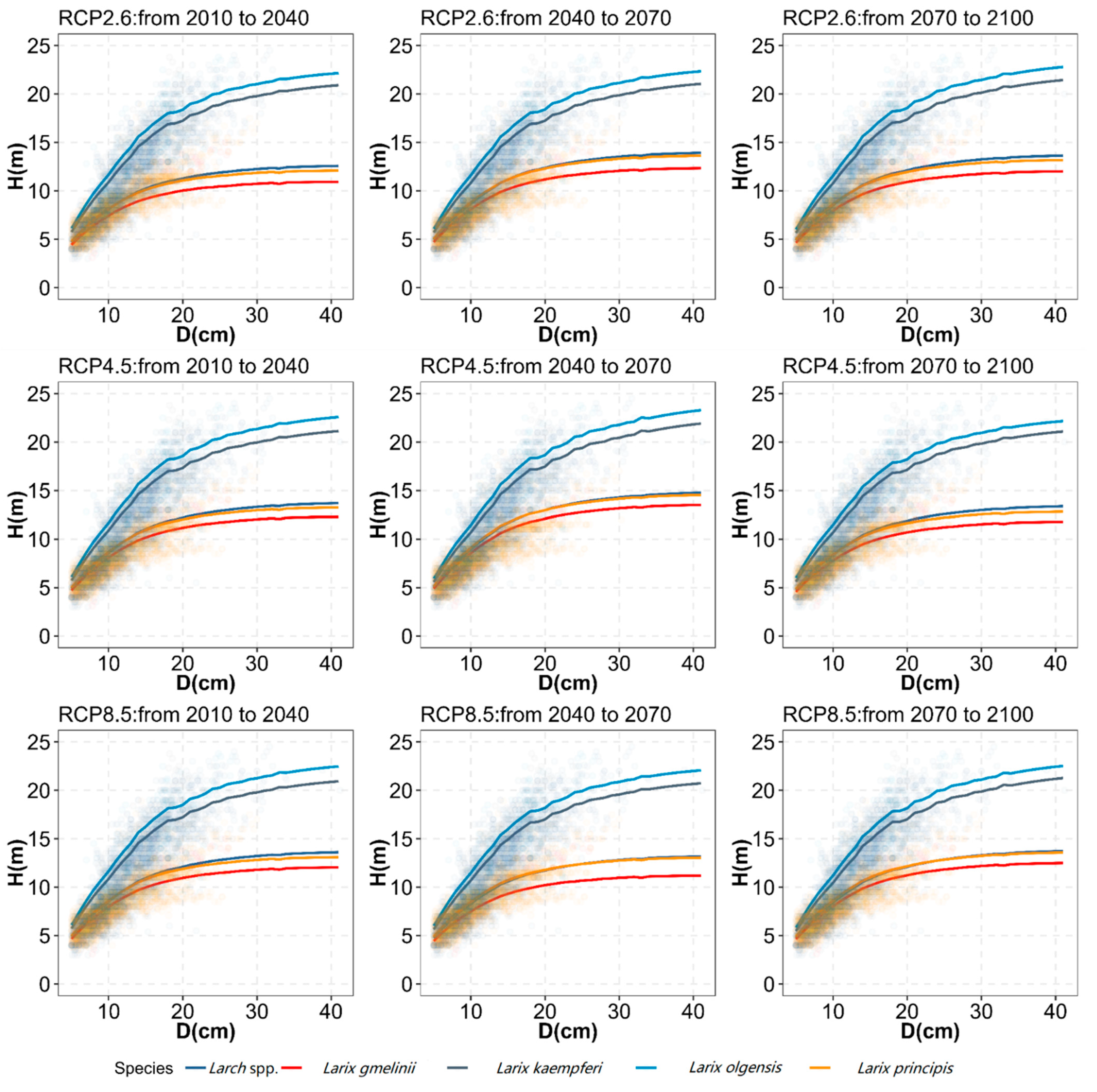
3.4. H–D Relationships among Larch Tree Species and Tree Sizes under Future Climate Change

Results showed different effects of climate variables on parameters a₀ and b₀, denoting the maximum and relative change of tree height with diameter (Table 6). Parameter a₁ was significantly negative indicating that the increasing BAL will reduce the maximum height. The coefficient a₂ of MAT for parameter a was significantly positive meaning that the rising MAT will increase the maximum tree height. This was also shown in Figure 3 where all H–D curves of different species became steeper under RCP2.6 and RCP 4.5 from 2010 to 2070. However, parameter b₂ was negative indicating that the rising MAT will lower the tree height with the same diameter and there is a threshold for the effect of temperature on H–D relationship of larch species. Parameter a₃ was significantly negative indicating the increase of CMD will reduce the maximum height. However, b₁ and b₃ were nearly zero and thus both CMD and BAL showed marginal effects on H–D relationship.

Table 6 showed that all parameters of tree species dummy variables g₁~g₄ were positive, but g₁ and g₄ were not significant, indicating that L. olgensis and L. kaempferi had a significant difference with the unidentified group, which was also illustrated in Figure 3. Coefficient g₂ was the largest indicating that the maximum tree height of L. olgensis was the largest.

MAT increased with the time and the temperature under RCP8.5 is the largest followed by RCP4.5 and RCP2.6. The precipitation under RCP8.5 is smallest and had the steepest slope followed by RCP4.5 and RCP2.6. Figure 4 showed that the $\mathsf{\Delta }$H–D curves of larch species under climate scenarios RCP2.6, RCP4.5 and RCP8.5. Generally, tree species can be obviously classified as two groups in terms of $\mathsf{\Delta }$H, which are group I (L. gmelinii, L. principis and the unidentified larch species) and group II (L. kaempferi and L. olgensis). They showed strong ($\mathsf{\Delta }$H ranged −4.77% to 18.17%) and weak ($\mathsf{\Delta }$H ranged −6.37% to 9.54%) responses to climate change, respectively. The values of $\mathsf{\Delta }$H for Group I were positive which indicated that future climate change increased tree height compared with current climate with the exception of RCP 2.6 from 2010 to 2040 and RCP8.5 from 2040–2100. However, the values of $\mathsf{\Delta }$H were complicated varying from negative to positive with the increasing diameter for Group II.

Figure 4 showed that $\mathsf{\Delta }$H varied with tree diameter. Generally, large trees showed large $\mathsf{\Delta }$H values, but there were different responses to the climate among larch species. For tree species group I, the $\mathsf{\Delta }$H increased with the increase of tree DBH in small and medium sizes and kept stable in large sizes. For group II, the absolute $\mathsf{\Delta }$H increased with the increase of tree DBH but changed from negative to positive.

Mean absolute $\mathsf{\Delta }$H values with diameter among larch species under different climate scenarios in period 2010 to 2100 (mean value of the absolute $\mathsf{\Delta }$H in period 2010 to 2040, 2040 to 2070 and 2070 to 2100) was shown in Figure 5. It can be observed that the climate sensitivity of larch species was ranked as L. gmelinii > L. principis > the unidentified species group > L. olgensis > L. kaempferi under RCP2.6 and RCP8.5, and the sensitivity was larger under RCP8.5 than that under RCP2.6. However, the sensitivity was ranked as L. gmelinii > the unidentified species group > L. principis > L. kaempferi > L. olgensis under RCP4.5.

4. Discussion

4.1. Climate-Sensitive H–D Model

The climate-sensitive H–D allometry model with a two-level NLME approach at the province and plot levels was developed for larch plantations in the study. Results showed that a two-level mixed-effects model with the inclusion of climate variables provided better performance compared to fixed-effects model without climate variables, which were consistent with other reports [7,10,11,12,13]. In this study, using the mixed-effects model and including climate variables increased $R_{adj}^2$ by 19.5% and reduced the AIC, MAE and RMSE by 22.2%, 44.5% and 41.8% for fitting data, respectively. The residual heterogeneity was also reduced. Owing to the correlation among tree height–diameter observations, fixed-effect model would lead to biased variance of the parameter estimates and thus invalidated the hypothesis tests [39]. The mixed-effect modelling approach can be an appropriate solution to this problem [5,40]. Similarly, Vizcaíno-Palomar et al. [41] reported that inclusion of climate variables and random effects reduced the AIC by 9.0%. Sharma et al. [40] reported that inclusion of random effects increased the $R_{adj}^2$ by 9.2% and the AIC and RMSE by 7.8% and 25%, respectively.

The climate variables including MAT and CMD significantly affected H–D relationship but the effect was not very strong which was in line with the previous studies [9,11,21]. Temperature usually affects the growth season and growth rate of tree height. Low temperature will hinder the division and specialization of cambium and meristem cells, thus accumulating more nutrients and carbohydrates and distributing them to the trunk. Therefore, the shape of tree changed [42]. Fortin et al. [21] pointed out that the mean temperature from March to September affected the H–D relationship of most French tree species. Temperature was not a marginal effect that can be overlooked and its effect was also quadratic so that an optimal temperature existed. Ng’andwe et al. [27] also found that increasing the temperature beyond the optimum for Pinus merkusii and P. michoacana reduced the tree growth and increased the rotation age. Similarly, in this study, MAT modified parameters a₂ and b₂ positively and negatively, respectively, which also indicated that there was an optimal temperature for larch tree height. Zhang et al. [11] reported that MAT was the dominant climatic factor in modulating height–diameter allometry of Chinese fir, and the effect of MAT and MWMT were positively associated with tree height of larch in the region begins to grow in May, and the growth speed reaches the maximum in July, then gradually slows down until it stops growing [43]. Therefore, the temperature in May and the precipitation in the previous year are very important for the height growth of larch. Our results showed that CMD had significant effects on H–D relationship. The coefficient of CMD, a₃, was negative which indicated that the height decreased with the increase of water deficiency. This was consistent with a previous study [44] which found that the precipitation from the previous October to the current April significantly promoted the height growth of Mongolian pine. Sang et al. [45] also found that the negative effects of CMD on the height of white spruce trees in northern Canada.

Besides climate, H–D relationship was affected by multiple biotic and abiotic variables, for example genetic characteristics [8], stand age [16], site condition [6,46], competition status [5,6]. Considering the inclusion of other stand factors will aggravate the model complexity, we only used diameter and BAL as the independent variable for ensuring more stable convergence. In addition, other methods such as machine learning were worthy of further exploration in future study.

4.2. The Impact of Climate Change on H–D Relationship by Larch Species and Tree Size

Our model simulations showed that the effects of climate change on H–D relationship varied with larch species. Generally, $\mathsf{\Delta }$H–D curves of larch species can be obviously classified as two groups, which are group I (L. gmelinii, L. principis and the unidentified species) and group II (L. kaempferi and L. olgensis). They showed strong ($\mathsf{\Delta }$H from −4.77% to 18.17%) and weak ($\mathsf{\Delta }$H from −6.37% to 9.54%) responses to future climate change, respectively. Under warmer and drier climatic conditions, L. kaempferi and L. ogensis will grow thicker and shorter than the rest of tree species group, and their $\mathsf{\Delta }$Hs were lower than those of group I for a given tree diameter. This may due to that these two tree species are moisture loving species [43]. Under drought stress, the hydraulic conductivity of the xylem of the trunk suffers irreversible loss. Therefore, the lack of water during the growing season allows to allocate more resources for the growth of diameter [47]. Compared with group II, group I is more resistant. As the temperature increases, more resources will be allocated to the growth of the height than the diameter, thus trees would be higher. Previous studies also supported this result [46,48,49,50].

$\mathsf{\Delta }$H also varied with tree diameter under future climate change. For tree species group I, $\Delta$H increased for small and medium sizes and kept stable for large sizes. This may be resulted from the limited height growth of trees with large diameter because of the limits to tree height [51]. For tree species group II, $\mathsf{\Delta }$H increased with the increasing DBH, but changed from negative to positive, indicating that small trees will grow short but large trees high. Campbell et al. [52] reported that large trees were most sensitive to annual climate fluctuations. From the perspective of competition, larger trees in a stand have more competitive advantages than smaller trees while the smaller neighbor trees do not influence the growth of larger trees [53]. Under the warmer and drier climate in the future, due to the developed root system of the big trees, their growth will not be affected by the lack of water, and the growth of small trees may face drought stress. McDowell et al. [54] pointed out that plants can avoid water damage caused by drought through stomatal closure, leading to carbon starvation and a cascade of down-stream effects. Seedlings or small trees are more likely to inhibit growth or even die due to hydraulic failure. The phenomena of changing from negative to positive for $\mathsf{\Delta }$H of L. kaempferi and L. olgensis along with increasing diameter supported this conclusion.

5. Conclusions

Two-level climate-sensitive NLME model was developed for larch plantations in north and northeast China which showed biological and statistical reasonability. MAT and CMD were the dominant climatic factors in modulating height–diameter allometry of larch plantations. Model simulations showed that the climate sensitivity of H–D allometry varied with tree species and diameter. According to the climate sensitivity, tree species could be classified as group I (L. gmelinii, L. principis and the unidentified species) with large $\mathsf{\Delta }\mathrm{H}$ (from −4.77% to 18.17%) and group II (L. kaempferi and L. olgensis) with small $\mathsf{\Delta }\mathrm{H}$ (from −6.37% to 9.54%). Large trees were more sensitive to climate change than small trees.

References

1. Zell, J. SwissStandSim: A Climate Sensitive Single TREE Stand Simulator for Switzerland: Schlussbericht im Forschungsprogramm Waldund Klimawandel; Swiss Federal Institute of Forest, Snow and Landscape Research: Birmensdorf, Switzerland, 2016. [Google Scholar]
2. Fang, Z.; Bailey, R. Height–diameter models for tropical forests on Hainan Island in southern China. For. Ecol. Manag. 1998, 110, 315–327. [Google Scholar] [CrossRef]
3. Huang, S.; Price, D.; Titus, S.J. Development of ecoregion-based height–diameter models for white spruce in boreal forests. For. Ecol. Manag. 2000, 129, 125–141. [Google Scholar] [CrossRef]
4. Jayaraman, K.; Zakrzewski, W. Practical approaches to calibrating height–diameter relationships for natural sugar maple stands in Ontario. For. Ecol. Manag. 2001, 148, 169–177. [Google Scholar] [CrossRef]
5. Calama, R.; Montero, G. Interregional nonlinear height diameter model with random coefficients for stone pine in Spain. Can. J. For. Res. 2004, 34, 150–163. [Google Scholar] [CrossRef] [Green Version]
6. Sharma, M.; Shu, Y.Z. Height–diameter models using stand characteristics for Pinus banksiana and Picea mariana. Scand. J. For. Res. 2004, 19, 442–451. [Google Scholar] [CrossRef]
7. Sharma, M.; Parton, J. Height–diameter equations for boreal tree species in Ontario using a mixed-effects modeling approach. For. Ecol. Manag. 2007, 249, 187–198. [Google Scholar] [CrossRef]
8. Kroon, J.; Andersson, B.; Mullin, T.J. Genetic variation in the diameter–height relationship in Scots pine (Pinus sylvestris). Can. J. For. Res. 2008, 38, 1493–1503. [Google Scholar] [CrossRef]
9. Hulshof, C.M.; Swenson, N.G.; Weiser, M.D. Tree height–diameter allometry across the United States. Ecol. Evol. 2015, 5, 1193–1204. [Google Scholar] [CrossRef] [PubMed]
10. Zang, H.; Lei, X.; Zeng, W. Height–diameter equations for larch plantations in northern and northeastern China: A comparison of the mixed-effects, quantile regression and generalized additive models. For. Int. J. For. Res. 2016, 89, 434–445. [Google Scholar] [CrossRef]
11. Zhang, X.; Chhin, S.; Fu, L.; Lu, L.; Duan, A.; Zhang, J. Climate-sensitive tree height–diameter allometry for Chinese fir in southern China. For. Int. J. For. Res. 2019, 92, 167–176. [Google Scholar] [CrossRef]
12. Bronisz, K.; Mehtätalo, L. Mixed-effects generalized height–diameter model for young silver birch stands on post-agricultural lands. For. Ecol. Manag. 2020, 460, 117901. [Google Scholar] [CrossRef]
13. Ciceu, A.; Garcia-Duro, J.; Seceleanu, I.; Badea, O. A generalized nonlinear mixed-effects height–diameter model for Norway spruce in mixed-uneven aged stands. For. Ecol. Manag. 2020, 477, 118507. [Google Scholar] [CrossRef]
14. Santiago-García, W.; Jacinto-Salinas, A.H.; Rodríguez-Ortiz, G.; Nava-Nava, A.; Santiago-García, E.; Ángeles-Pérez, G.; Enríquez-del Valle, J.R. Generalized height-diameter models for five pine species at Southern Mexico. For. Sci. Technol. 2020, 16, 49–55. [Google Scholar] [CrossRef]
15. Zhang, B.; Sajjad, S.; Chen, K.; Zhou, L.; Zhang, Y.; Yong, K.K.; Sun, Y. Predicting Tree Height-Diameter Relationship from Relative Competition Levels Using Quantile Regression Models for Chinese Fir (Cunninghamia lanceolata) in Fujian Province, China. Forests 2020, 11, 183. [Google Scholar] [CrossRef] [Green Version]
16. Sánchez, C.A.L.; Varela, J.G.; Dorado, F.C.; Alboreca, A.R.; Soalleiro, R.R.; González, J.G.Á.; Rodríguez, F.S. A height-diameter model for Pinus radiata D. Don in Galicia (Northwest Spain). Ann. For. Sci. 2003, 60, 237–245. [Google Scholar] [CrossRef]
17. Krisnawati, H.; Wang, Y.; Ades, P.K. Generalized height-diameter models for Acacia mangium Willd. plantations in south Sumatra. Indones. J. For. Res. 2010, 7, 1–19. [Google Scholar]
18. Saunders, M.R.; Wagner, R.G. Height-diameter models with random coefficients and site variables for tree species of Central Maine. Ann. For. Sci. 2008, 65, 203. [Google Scholar] [CrossRef] [Green Version]
19. Russell, M.B.; Amateis, R.L.; Burkhart, H.E. Implementing regional locale and thinning response in the loblolly pine height-diameter relationship. South. J. Appl. For. 2010, 34, 21–27. [Google Scholar] [CrossRef] [Green Version]
20. Wang, X.; Fang, J.; Tang, Z.; Zhu, B. Climatic control of primary forest structure and DBH–height allometry in Northeast China. For. Ecol. Manag. 2006, 234, 264–274. [Google Scholar] [CrossRef]
21. Fortin, M.; Van Couwenberghe, R.; Perez, V.; Piedallu, C. Evidence of climate effects on the height-diameter relationships of tree species. Ann. For. Sci. 2019, 76, 1. [Google Scholar] [CrossRef] [Green Version]
22. Kirschbaum, M.U. Forest growth and species distribution in a changing climate. Tree Physiol. 2000, 20, 309–322. [Google Scholar] [CrossRef] [PubMed]
23. Yang, Y.; Watanabe, M.; Li, F.; Zhang, J.; Zhang, W.; Zhai, J. Factors affecting forest growth and possible effects of climate change in the Taihang Mountains, northern China. For. Int. J. For. Res. 2006, 79, 135–147. [Google Scholar] [CrossRef] [Green Version]
24. Hartl-Meier, C.; Dittmar, C.; Zang, C.; Rothe, A. Mountain forest growth response to climate change in the Northern Limestone Alps. Trees 2014, 28, 819–829. [Google Scholar] [CrossRef]
25. Charney, N.D.; Babst, F.; Poulter, B.; Record, S.; Trouet, V.M.; Frank, D.; Enquist, B.J.; Evans, M.E. Observed forest sensitivity to climate implies large changes in 21st century North American forest growth. Ecol. Lett. 2016, 19, 1119–1128. [Google Scholar] [CrossRef]
26. Albert, M.; Schmidt, M. Climate-sensitive modelling of site-productivity relationships for Norway spruce (Picea abies (L.) Karst.) and common beech (Fagus sylvatica L.). For. Ecol. Manag. 2010, 259, 739–749. [Google Scholar] [CrossRef]
27. Ng’andwe, P.; Chungu, D.; Tailoka, F. Stand characteristics and climate modulate height to diameter relationship in Pinus merkusii and P. michoacana in Zambia. Agric. For. Meteorol. 2021, 307, 108510. [Google Scholar] [CrossRef]
28. Feldpausch, T.R.; Banin, L.; Phillips, O.L.; Baker, T.R.; Lewis, S.L.; Quesada, C.A.; Affum-Baffoe, K.; Arets, E.J.; Berry, N.J.; Bird, M. Height-diameter allometry of tropical forest trees. Biogeosciences 2011, 8, 1081–1106. [Google Scholar] [CrossRef] [Green Version]
29. State Forestry Administration, The People’s Republic of China. National Forest Resources Statistics (2009–2013); State Forestry Administration: Beijing, China, 2014; p. 233.
30. Shen, C.; Lei, X.; Liu, H.; Wang, L.; Liang, W. Potential impacts of regional climate change on site productivity of Larix olgensis plantations in northeast China. ifor.-Biogeosci. For. 2015, 8, 642. [Google Scholar] [CrossRef] [Green Version]
31. Xie, Y.; Wang, H.; Lei, X. Application of the 3-PG model to predict growth of Larix olgensis plantations in northeastern China. For. Ecol. Manag. 2017, 406, 208–218. [Google Scholar] [CrossRef]
32. Xie, Y.; Lei, X.; Shi, J. Impacts of climate change on biological rotation of Larix olgensis plantations for timber production and carbon storage in northeast China using the 3-PGmix model. Ecol. Model. 2020, 435, 109267. [Google Scholar] [CrossRef]
33. Lei, X.; Yu, L.; Hong, L. Climate-sensitive integrated stand growth model (CS-ISGM) of Changbai larch (Larix olgensis) plantations. For. Ecol. Manag. 2016, 376, 265–275. [Google Scholar] [CrossRef]
34. Wang, T.; Wang, G.; Innes, J.L.; Seely, B.; Chen, B. ClimateAP: An application for dynamic local downscaling of historical and future climate data in Asia Pacific. Front. Agric. Sci. Eng. 2017, 4, 448–458. [Google Scholar] [CrossRef] [Green Version]
35. Van Vuuren, D.P.; Edmonds, J.; Kainuma, M.; Riahi, K.; Thomson, A.; Hibbard, K.; Hurtt, G.C.; Kram, T.; Krey, V.; Lamarque, J.-F. The representative concentration pathways: An overview. Clim. Chang. 2011, 109, 5. [Google Scholar] [CrossRef]
36. Voldoire, A.; Sanchez-Gomez, E.; y Mélia, D.S.; Decharme, B.; Cassou, C.; Sénési, S.; Valcke, S.; Beau, I.; Alias, A.; Chevallier, M. The CNRM-CM5.1 global climate model: Description and basic evaluation. Clim. Dyn. 2013, 40, 2091–2121. [Google Scholar] [CrossRef] [Green Version]
37. Wold, S.; Esbensen, K.; Geladi, P. Principal component analysis. Chemom. Intell. Lab. Syst. 1987, 2, 37–52. [Google Scholar] [CrossRef]
38. Scolforo, J.R.S.; Maestri, R.; Ferraz Filho, A.C.; de Mello, J.M.; de Oliveira, A.D.; de Assis, A.L. Dominant height model for site classification of Eucalyptus grandis incorporating climatic variables. Int. J. For. Res. 2013, 2013, 139236. [Google Scholar]
39. Pinheiro, J.; Bates, D.; DebRoy, S.; Sarkar, D.; Team, R.C. nlme: Linear and nonlinear mixed effects models. R Package Version 2013, 3, 111. [Google Scholar]
40. Sharma, R.; Vacek, Z.; Vacek, S. Nonlinear mixed effect height-diameter model for mixed species forests in the central part of the Czech Republic. J. For. Sci. 2016, 62, 470–484. [Google Scholar]
41. Vizcaíno-Palomar, N.; Ibáñez, I.; Benito-Garzón, M.; González-Martínez, S.C.; Zavala, M.A.; Alía, R. Climate and population origin shape pine tree height-diameter allometry. New For. 2017, 48, 363–379. [Google Scholar] [CrossRef]
42. Kilpeläinen, A.; Peltola, H.; Rouvinen, I.; Kellomäki, S. Dynamics of daily height growth in Scots pine trees at elevated temperature and CO2. Trees 2006, 20, 16–27. [Google Scholar] [CrossRef]
43. Wang, Z.; Wang, S.; Wang, G.; Wang, C.; Bai, T.; Lu, H.; Lv, H.; Chen, C.; Yuan, J.; Xu, Z.; et al. Larch Forest in China; China Forestry Publishing House: Beijing, China, 1992. [Google Scholar]
44. Zhou, Y.; Lei, Z.; Zhou, F.; Han, Y.; Yu, D.; Zhang, Y. Impact of climate factors on height growth of Pinus sylvestris var. mongolica. PLoS ONE 2019, 14, e0213509. [Google Scholar] [CrossRef] [PubMed] [Green Version]
45. Sang, Z.; Sebastian-Azcona, J.; Hamann, A.; Menzel, A.; Hacke, U. Adaptive limitations of white spruce populations to drought imply vulnerability to climate change in its western range. Evol. Appl. 2019, 12, 1850–1860. [Google Scholar] [CrossRef] [PubMed] [Green Version]
46. Zhang, X.; Wang, H.; Chhin, S.; Zhang, J. Effects of competition, age and climate on tree slenderness of Chinese fir plantations in southern China. For. Ecol. Manag. 2020, 458, 117815. [Google Scholar] [CrossRef]
47. Ryan, M.G.; Yoder, B. Hydraulic limits to tree height and tree growth. Bioscience 1997, 47, 235–242. [Google Scholar] [CrossRef] [Green Version]
48. Aiba, S.-i.; Kitayama, K. Structure, composition and species diversity in an altitude-substrate matrix of rain forest tree communities on Mount Kinabalu, Borneo. Plant Ecol. 1999, 140, 139–157. [Google Scholar] [CrossRef]
49. Thornley, J.H. Modelling stem height and diameter growth in plants. Ann. Bot. 1999, 84, 195–205. [Google Scholar] [CrossRef] [Green Version]
50. Schelhaas, M. The wind stability of different silvicultural systems for Douglas-fir in the Netherlands: A model-based approach. Forestry 2008, 81, 399–414. [Google Scholar] [CrossRef] [Green Version]
51. Koch, G.W.; Sillett, S.C.; Jennings, G.M.; Davis, S.D. The limits to tree height. Nature 2004, 428, 851–854. [Google Scholar] [CrossRef]
52. Campbell, E.M.; Magnussen, S.; Antos, J.A.; Parish, R. Size-, species-, and site-specific tree growth responses to climate variability in old-growth subalpine forests. Ecosphere 2021, 12, e03529. [Google Scholar] [CrossRef]
53. Cannell, M.; Rothery, P.; Ford, E. Competition within stands of Picea sitchensis and Pinus contorta. Ann. Bot. 1984, 53, 349–362. [Google Scholar] [CrossRef] [Green Version]
54. McDowell, N.; Pockman, W.T.; Allen, C.D.; Breshears, D.D.; Cobb, N.; Kolb, T.; Plaut, J.; Sperry, J.; West, A.; Williams, D.G. Mechanisms of plant survival and mortality during drought: Why do some plants survive while others succumb to drought? New Phytol. 2008, 178, 719–739. [Google Scholar] [CrossRef]
Figure 1. Scatter plots of tree height–diameter allometry by larch species in 7 provinces.
Forests 13 00468 g001
Figure 2. Residuals distribution for different H–D models based on calibration data.
Forests 13 00468 g002
Figure 3. Relationship between tree height and DBH of larch species under different climate change scenarios.
Forests 13 00468 g003
Figure 4. Relative change of tree height with diameter among larch species under different climate scenarios.
Forests 13 00468 g004
Figure 5. Mean absolute Δ H values of height with diameter among larch species under different climate scenarios.
Forests 13 00468 g005