Article

The Effect of Stand Density, Biodiversity, and Spatial Structure on Stand Basal Area Increment in Natural Spruce-Fir-Broadleaf Mixed Forests

1
Research Institute of Forest Resource Information Techniques, Chinese Academy of Forestry, Beijing 100091, China
2
Key Laboratory of Forest Management and Growth Modeling, National Forestry and Grassland Administration, Beijing 100091, China
3
Experimental Center of Forestry in North China, Chinese Academy of Forestry, No.1 Shuizha West Road, Mentougou District, Beijing 102300, China
*
Author to whom correspondence should be addressed.
Forests 2022, 13(2), 162; https://doi.org/10.3390/f13020162
Submission received: 26 November 2021 / Revised: 27 December 2021 / Accepted: 30 December 2021 / Published: 21 January 2022
(This article belongs to the Special Issue Advances in Forest Growth and Site Productivity Modeling)

Abstract

:
Forest trees exhibit a large variation in the basal area increment (BAI), and the variation is attributed to the stand density, biodiversity, and stand spatial structure. Studying and quantifying the effect of these above variables on tree growth is vital for future forest management. However, the stand spatial structure based on neighboring trees has rarely been considered, especially in the mixed forests. This study adopted the random-forest (RF) algorithm to model and interpret BAI based on stand density, biodiversity, and spatial structure. Fourteen independent variables, including two stand density predictors, four biodiversity predictors, and eight spatial structure predictors, were evaluated. The RF model was trained for the whole stand, three tree species groups (gap, neutral, and shade_tolerant), and two tree species (spruce and fir). A 10-fold blocked cross-validation was then used to optimize the hyper-parameters and evaluate the models. The squared correlation coefficients (R2) for the six groups were 0.233 for the whole stand, 0.575 for fir, 0.609 for shade_tolerant, 0.622 for neutral, 0.722 for gap, and 0.730 for spruce. The Stand Density Index (SDI) was the most-important predictor, suggesting that BAI is primarily restricted by competition. BAI and species biodiversity were positively correlated for the whole stand. The stands were expected to be randomly distributed based on the relationship between the uniform angle index (W) and growth. The relationship between dominance (U) and BAI indicated that small trees should be planted around the light-demanding tree species and vice versa. Of note, these findings emphasize the need to consider the three types of variables in mixed forests, especially the spatial structure factors. This study may help make significant advances in species composition, spatial arrangement, and the sustainable development of mixed forests.

1. Introduction

Understanding forest growth is crucial for forest management and the estimations of net primary production and carbon sequestration [1]. Forests with mixed species have higher productivity, higher temporal stability, a lower risk of biotic and abiotic disturbances, and a more diverse ecosystem. However, it is challenging to model their growth because of complex communities [2]. Basal area growth increment (BAI) is particularly suitable for modelling tree growth among the other measurements because it is directly related to the diameter at breast height (DBH), thus making it more reliable [3,4]. Machine-learning algorithms have already been used in forest management, providing more accurate predictions than the traditional linear regressions in dendroclimatology [5,6,7,8,9]. Notably, Martin Jung used BAI modelling of spruce and fir in random forests [10].
The role of stand biodiversity for ecosystem processes, such as biomass production, nutrient storage as well as energy and material flow, is currently the most demanding ecological research topic, especially in the context of climate change [11]. Numerous indicators have been developed to measure species and structural diversity to enable local and temporal comparisons [12]. Studies of the relationship between forest diversity and productivity in various forest ecosystems have revealed positive, neutral, and negative correlations [13]. Moreover, the impact of species diversity on productivity is controversial, especially in forest communities with complicated spatial structures and long life spans of dominant organisms [14]. The scale and stand development stage evaluated must therefore be considered when discussing diversity [15,16]. Density is also a foundational component of forest growth models. Density measurements combining the use of growing areas with the size of the trees are required when comparing stands of different forest ages or different locations [17]. Strikingly, the Stand Density Index (SDI) proposed by Reineke (1933) is the most commonly used measurement method. It accounts for the number and average diameter of trees based on the allometric relationship between these two variables to express the tree number as a reference quadratic mean diameter [18]. The SDI has been used in a great deal of forest growth models for its simplicity [19,20,21]. However, there are very limited studies available regarding SDI on BAI, and additional research is needed.
The forest structure is a dominant feature of forests, reflecting the connection among individual trees, their regeneration patterns, and their competition. It thus plays a crucial role in the natural dynamics of ecosystem [22,23,24]. There are various methods available for measuring forest structure. Among them, a quantization method based on a basic unit (a reference tree with its four nearest trees) is accepted and widely used in quantifying forest structure [25,26,27], which is defined as spatial structural unit. The uniform angle index (W) [28], dominance (U) [29], mingling (M) [30], and crowding (C) [31] can be calculated based on the spatial structural unit. The four structural parameters accurately express the relative size of individuals, the spatial pattern of neighbor trees, tree species mingling, and whether they have horizontal competition [32]. The optimal stand spatial state is a significant factor to the development of forest growth [33]. Some cross-sectional studies found that individual density of neighboring trees or the same species, the size distribution, and the number of relative species significantly associate with the growth of target trees [34,35]. However, there have been surprisingly few historical studies on the relationship between growth and spatial structure through the model.
This study aimed to (1) explore and evaluate a machine-learning model for BAI predictions for the whole stand, tree species. and tree species groups in the north-eastern area of China; (2) identify the main predictor variables; and (3) interpret the effect of key predictors of forest structure on BAI and provide guidance for forest management.

2. Materials and Methods

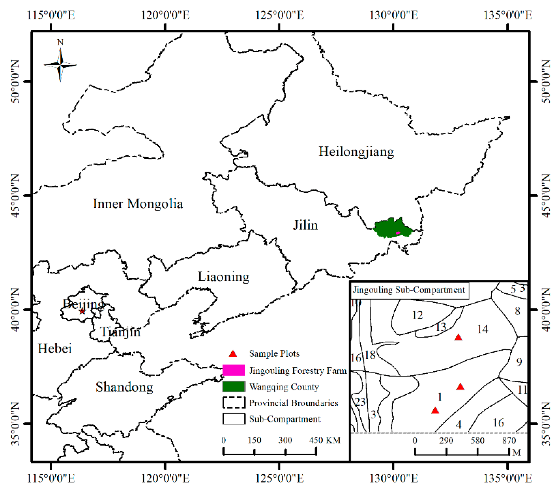
2.1. Study Area and Experimental Design

The study area was located in the Jingouling Forest Farm in the northeast of Wangqing County, Jilin Province, in the low hilly area of the Changbai Mountains. The altitude of the study area is 300–1200 m, with its slope is mainly concentrated at 5°–25°. The region has a temperate continental monsoon climate with four distinct seasons, with temperatures ranging from −32 °C to 32 °C and annual average rainfall from 600 mm to 700 mm. The early frost starts in mid-September, and the late frost extends to the end of May of the following year. The growth period is 120 days, and the average snow cover is 50 cm thick. The coniferous gray-brown loamy soil is dominant, with a thickness of about 45 cm harboring high natural fertility. The parent rock is basalt, with a moist and loose granular structure and an acidic pH. This study adopted spruce-fir natural forest as an example, with the study area being a typical representative of over-deforestation.
One-hectare sampling plots (100 m × 100 m) were established in a spruce-fir-broadleaf mixed forest in 2013 (Figure 1 and Table 1). All live trees with diameters at breast height (DBH) ≥ 1 cm in each plot were recorded. Their locations were then mapped, their species identified, and their DBH, height (H), crown diameter, and clear bole height were measured. Remeasurements were done in 2018, five years after the study began. Three control plots were then selected and divided into 75 small plots, measuring 20 × 20 m. The translation method is used for edge-correction [36]. Tree samples with ≥5 cm diameter at breast height (DBH) were then used to calculate the stand basal area, spatial-structure parameters, species-diversity indices, and stand-structure indices. The remaining records were finally obtained for analysis, excluding the plots where the stand basal area was inverted. Tree data collected from 2013 to 2018 were used for stand basal area prediction.

2.2. Predictor Variables

The predictor variables were consolidated into three groups: (1) spatial-structure parameters, (2) biodiversity indices, and (3) forest stand characteristics. Four forest spatial-structure parameters based on the spatial structural unit were used as the spatial-structure parameters. They included the uniform angle index (W), describing the degree of tree distribution uniformity; dominance (U), reflecting the degree of DBH differentiation; mingling (M), expressing the degree of tree species segregation; and crowding (C), reflecting the degree of tree crowding. Tree species diversity, tree size diversity, and the integrated diversity index of tree species and size were used as the biodiversity indices, whilst Reineke’s stand density index (SDI) was used to measure the stand characteristics. Table 2 highlights the final set of independent variables with descriptive statistics.

2.3. Random-Forest Algorithm for Predicting Stand Basal Area Increment (BAI)

The random forest (RF), a nonparametric, data-driven method based on an ensemble of bootstrapped classification or regression trees, was the primary modelling tool used in this study. The excellent predictive power of the random-forest algorithm is based on the construction of a random regression tree for each bootstrapping sample. At each tree node, only a subset of all nodes is divided, taking into account the available independent variables. This subset is defined with the parameter mtry. The mtry specifies the number of variables to randomly selected and tested at each node of each tree. The tool employs three steps to implement the regression: (1) Bootstrap is used to sample the original training set (n × p) to get k training sets (n × p); (2) a regression tree model for k training sets is then built separately to get k regression results; (3) finally, the average of k regression results is taken as the final prediction result [37]. RF improves prediction accuracy by integrating multiple regression trees; it has the ability to fit nonlinear functions; and it can improve the interpretability of the model by measuring the relative importance of independent variables [38]. We used the R RandomForest package to implement the RF algorithm for modelling BAI [39].
Predictive BAI models were developed for six groups: whole stand, gap, neutral, shade_tolerant, spruce (Picea jezoensis), and fir (Abies nephrolepis), with gap stands for light-demanding tree species, neutral stands for neutral tree species, and shade_tolerant stands for shade-tolerant tree species (Table 3).
The forest stand density, biodiversity, and spatial-structure factors were used as input variables of RF to establish the BAI regression model. The variance inflation factor was first used to determine the collinearity and to remove the variables from the final model accordingly (variance inflation factor >10) to exclude strongly related variables and to avoid introducing unnecessary parameters [40]. All predictor variables were used to train the RF model for each group independently based on the value of mtry parameters between 2 and 14. A 10-fold blocked cross-validation was then used to optimize hyper-parameters and to evaluate the BAI models. The squared correlation coefficient (R2) and the mean square error (RMSE) were averaged across the 10 validation folds. For each group, the highest R2 was selected and used for further analysis.

3. Results

3.1. Random Forest Model Evaluation

Spruce had the highest performance (R2: 0.730), while the whole stand had the lowest performance (R2: 0.223) (Table 4). In general, the tree species group (gap with mtry = 8, neutral with mtry = 10, and shade_tolerant with mtry = 14) and the tree species (spruce with mtry = 11 and fir with mtry = 14) had higher fitting accuracy than the whole stand.

3.2. The Relative Importance (%) of Predictors

The most-important predictors of each variable were determined based on performance during prediction (Table 5). SDI ranked as the top discriminative predictor for the whole stand, demonstrating its effectiveness for BAI. Four spatial-structure predictors explained 51.86% of all in total. Um had the largest proportion (21.18%), explaining almost the same amount of SDI. SDI explained 50.69%, while biodiversity explained 22.41% of all in the gap. As regards spatial-structure predictors, Mm_part had the largest proportion (7.97%) among the spatial-structure predictors. In the same line, SDI explained 38.28%, 53.27%, and 52.58% for neutral, shade_tolerant, and spruce, respectively. Compared with gap, Um_part (8.56%) accounted for the largest proportion ahead of Mm_part (8.04%) in shade_tolerant. However, SDI (24.98%) had the largest contribution than Mm_part (15.37%) in fir.

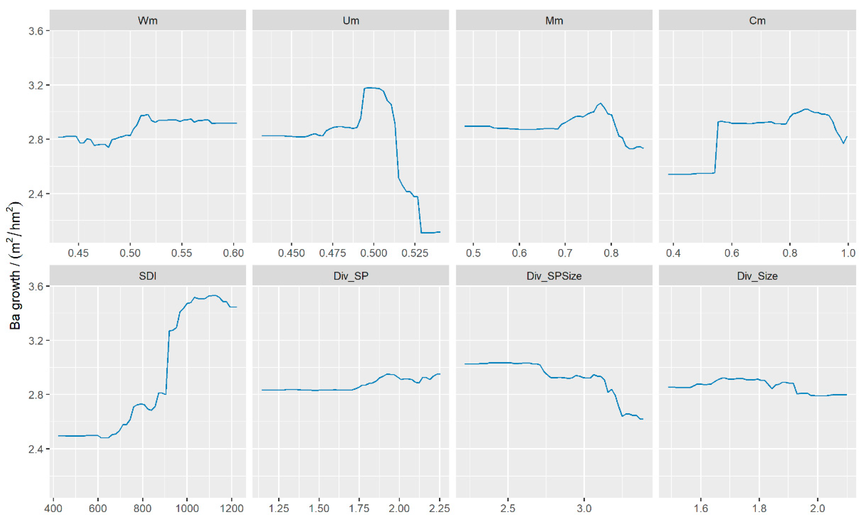
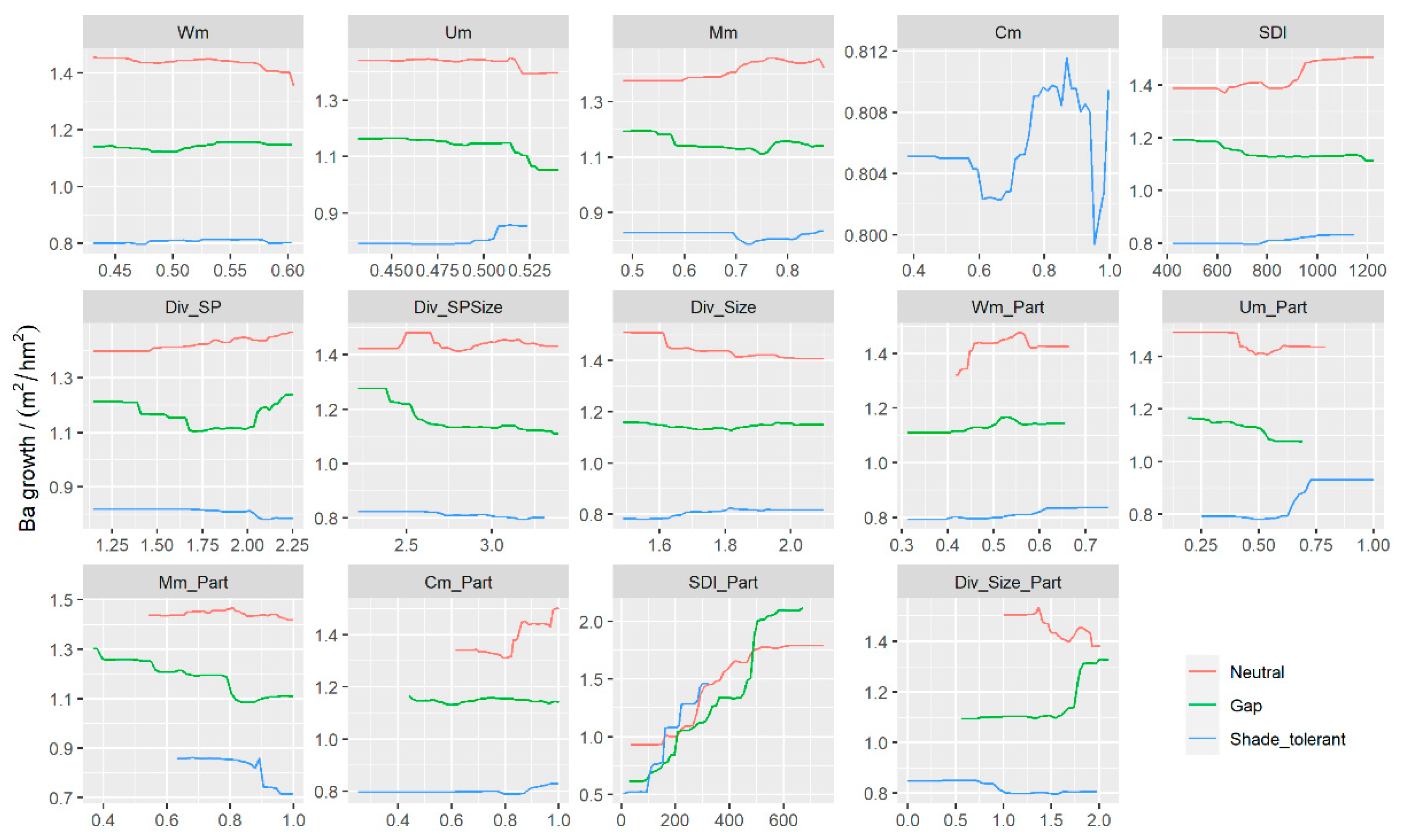
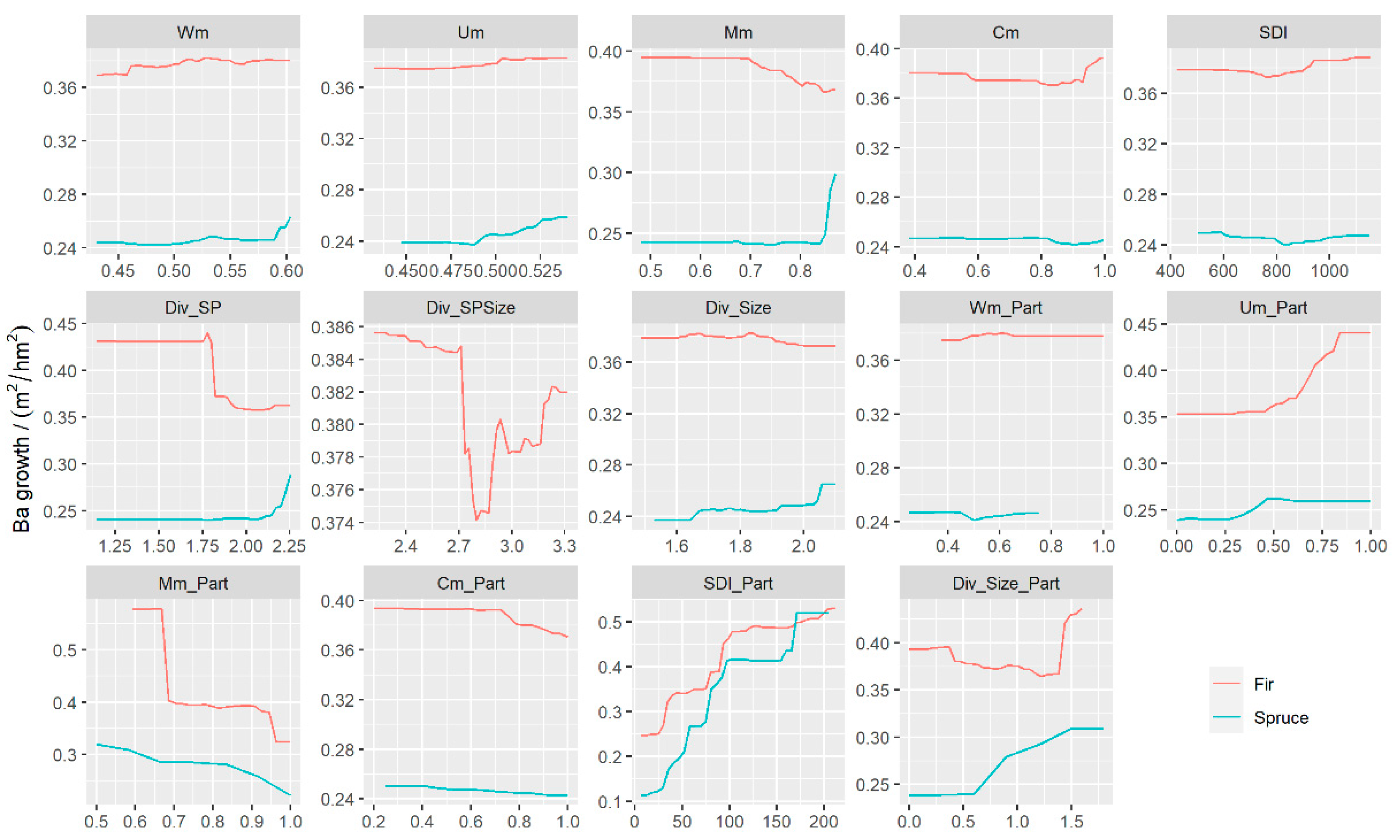
3.3. The Effects of Predictors on BAI

SDI was the most-important variable for BAI for whole stand, gap, neutral, shade_tolerant, fir, and spruce. It had a strong positive effect on BAI, but when SDI in whole stand (Figure 2) and SDI_part in tree species groups (Figure 3) or tree species (Figure 4) reached the threshold, BAI stopped increasing and became a constant. For whole stand, gap, neutral, and shade_tolerant, the inflection points were approximately 1000, 500, 500, and 300, respectively. For fir and spruce, this point was reached relatively early (Figure 2, Figure 3, and Figure 4).
For whole stand (Figure 2), Um was the most-important predictor of the stand spatial structure. BAI first increased and surpassed a maximum and then decreased as Um increased. BAI increased with the increase in Mm and surpassed a maximum and then decreased. BAI increased slowly with the increase in Wm and then became constant at a maximum value of 0.517. However, BAI increased sharply when Cm took a value between 0.5 and 0.6. When it came to Div_SPSize, there was a clear trend of decreasing at the late of the curve. In contrast, Div_Size had little discernible influence on BAI. When Div_SP was between 1.75 to 2.25, BAI increased gradually with a slight fluctuation.
When considering Wm_part, neutral had a greater impact on BAI than gap and shade_tolerant. The BAI of gap decreased first and then gradually stabilized with the increase in Um_Part in gap, while the BAI of shade_tolerant increased first (after a period of quiescent stability) and then tended to be stable with the increase in Um_Part in shade_tolerant (Figure 3). Cm_Part of neutral with values predominantly distributed among 0.6 and 1.0, which was positively correlated with the BAI of neutral. By comparison, Cm_Part of gap and Cm_Part of shade_tolerant had less influence on BAI. When it came to Mm_Part, the relationship between BAI and neutral was relatively weak; however, BAI was negatively correlated with gap and shade_tolerant. The effects of the four diversity indicators on shade_tolerant were negligible. For Div_Size_Part, the effects of gap and neutral were inconsistent.
The BAI of fir and spruce first stayed constant and then increased and finally stabilized with the increase in Um_part (Figure 4). Although fir and spruce of Mm_Part were negatively correlated with BAI, the influence of fir was more significant. The BAI of fir did not change with Div_SP at the beginning, and when the value of Div_SP reached 1.75, BAI dropped. However, the effect of Div_SP on the BAI of spruce could be negligible. The response of fir BAI and spruce BAI to Div_Size_Part were inconsistent. Consistent with Wm_part, Cm_part also promoted a very weak response to the BAI in fir and spruce.

4. Discussion

4.1. Evaluation of Random-Forest Model

The explained variance is usually lower in mixed-species unevenly aged forests than that in even-aged pure stands [2]. This result is attributed to the significant differences in the growth of various tree species in the mixed forest, which causes difficulties in prediction. In our study, tree species (spruce and fir) and tree species group (gap, neutral, and shade_tolerant) had better results than the whole stand in BAI modelling. This finding was attributed to the varying responses of different tree species to spatial structure, stand structure, and density [41]. A better simulation effect was further achieved by dividing the forest stand into tree-species groups. This view was supported by Ni et al. [42], who also found that the division is necessary for analyzing the mixed species stand by grouping species.

4.2. The Effects of STAND Density and Biodiversity on BAI

Stand BAI tends to increase with an increase in stand density and then stabilizes after the tree crown has peaked [43]. SDI (Figure 2) or SDI_part (Figure 3 and Figure 4) follows the same trend in the nature mixed forests. The reason for this and the possible underlying mechanism were investigated. Tree growth is rarely restricted by competition during early stand development because the resources are sufficient. Increasing dominance near canopy closure reduces the efficiency of resource use by non-dominant trees, lowering overall stand growth. The hierarchical structure of the tree during late stand development creates a spatial heterogeneity of the light resources, causing several species to coexist by compromising their demographic parameters.
Tree species diversity, tree size diversity, and the integrated diversity index of tree species and size were used in our study. The positive correlation observed between the BAI and species diversity (Figure 2) was consistent with the findings of several previous studies [44]. This effect was related to full utilization of natural resources in stands with higher tree species diversity. The trends of tree species diversity and integrated diversity index of tree species and size were opposite at the whole stand level (Figure 2). Moreover, the relationship between the BAI and the integrated diversity index of tree species and size was less clear, whereas the BAI was weakly correlated with tree size diversity (Figure 2), essentially because the largest trees do not counterbalance the lesser growth of the smaller trees in uneven-aged forests compared with even-aged forests.

4.3. Simulated Effect of Forest Spatial Structure Variables on BAI Prediction

The growth and production of mixed forest stands have become a popular research topic as these types of forests have functional and service advantages [17]. Spatial structures are of paramount importance in community research because their existence suggests their formation process [45]. The importance of structure on forest processes highlights the value of understanding the relationship between stand structure and growth and how this relationship is influenced by tree crowding and relative tree size, species mixing, and spatial distribution. Analyzing the growth of mixed stands requires a modelling approach that relates the growth of individual trees to their resource availability and provides output values per species [46]. In recent years, a group of neighborhood-based structural parameters with strong functionality that can fully express the spatial-structural features of tree populations and forest communities, and that can guide forestry practices, has attracted widespread attention [47]. Previous studies have mainly focused on the univariate distribution and mean value of the structural parameters to analyze the structural properties of stands. Several studies have further analyzed the influence of a horizontal spatial distribution and species mingling on stand growth in mixed forest using individual tree models [48,49]. However, only a few empirical-based studies have been conducted to assess these effects at the stand level. Neighboring trees may be able to improve the predictions of the model. Models with spatially explicit structural indices perform better than those with non-spatial indices due to the complexity of the stand structure [50]. Furthermore, relationships between stand growth and a given structural variable can vary widely depending on the forest types and species [38].
Spatial-distribution patterns reflect the way individuals gather or disperse on the horizon and determine the distribution of microclimatic conditions, the availability of resources, and the formation of habitat niches; thus, they significantly influence the biological diversity, tree growth, and timber production [51]. Generally, the spatial structures of natural forests always follow random distributions in horizontal space. Such a spatial distribution may be quantified using an area-independent nearest-neighborhood uniform-angle index (W) proposed by Gadow and Hui (1999), and if the W-mean belongs to the confidence interval (0.475, 0.517), the distribution pattern is random; otherwise, the pattern is classified as clumped (W-mean > 0.517) or regular (W-mean < 0.475) [25]. Our results suggest that the maximum value of Wm is 0.517 at the whole stand level, and this value is in the range of a random distribution (0.475, 0.517). It confirms that a random distribution is beneficial to the accumulation of forest stand area. Additionally, Zhang (2018) showed that random-structure units provide the majority of the BAI, whereas uniform and cluster structure units account only for a small part of the basal area [21].
Dominance (U) between trees plays a significant role within a stand and affects the fate of each plant. The spatial heterogeneity of light resources created by a tree hierarchy allows multiple species to coexist by means of trade-offs between demographic parameters [52]. Stand growth may increase, decrease, or remain unchanged with U, which has the advantage of quantifying plant growth among trees of different sizes within the stand [38]. U can be simply described as the number of large trees around the subject tree. One interesting finding is the BAI of gap decreases first and then gradually stabilizes at 0.5 with the increases in Um_Part in gap, and the BAI of shade_tolerant increases first and then tends to be stable at 0.75 with the increases in Um_Part in shade_tolerant. This means that if a light-demanding tree species is used as a target tree, its BAI becomes lager when its neighboring tree is a small tree. However, the shade-tolerant tree species expects the number of large trees around it to be greater than that of small trees. The growth of the light-demanding tree species needs light, so the small trees surrounding it that do not block it are more suitable for its growth, while the surrounding large trees can provide a canopy environment for shade-tolerant tree species, which is more conducive to its growth. Our study proves that the light-demanding tree species has a large BAI in the open, and the shade-tolerant tree species has a large BAI when the canopy is covered from the perspective of spatial-structure parameters.
Species mingling refers to the segregation of different species in the same community, which can describe the dissimilarity of tree species based on a reference tree and a set of neighboring trees, and the degree of mixing determines the state of light and the composition of litter, which in turn influences the growth and regeneration of trees [53]. The species-mingling value at the tree level varies inversely with the relative density of each tree species. The more uniform the trees are collected at the stand level, the lower the mixing rate between species. The species-mingling index has been used to determine the influence of structure-based forest-management methods on the spatial structure of forest stands. The focus has been put on the effects of species mixing on growth and the interactions between trees that cause such effects [13]. However, the effects of species mixing on growth largely depend on stand structure. In this contribution, species-mixing and BAI were negatively correlated in all cases except whole stand, suggesting trees with similar properties occurring in groups rather than alone have a larger BAI. However, for the whole stand, with the increases in Mm, BAI first increases, passes a maximum, and then decreases. This result clearly shows that it is not that the higher the degree of mixing, the greater the growth of the forest, but that there is a threshold, that is, the maximum growth of the forest is when there are three different trees around the target tree. Another important point here is that the implication of mingling (M) based on neighboring trees and species diversity are distinguished.
The degree of stand crowdedness is easy and convenient to evaluate and determines whether the forest requires to be cultivated, the time for the first thinning, and the cutting intensity. The crowding degree (C) of trees based on the relationship of neighboring trees was proposed by Hu and Hui [28]. Only limited information was found in the literature on C. Notably, the neutral tree species has the greatest correlation between BAI and Cm. This finding may mean that neutral tree species are the most sensitive to competition. Nevertheless, further work is required to establish the relationship between growth and crowding.
Collectively, (1) BAI and species diversity are positively correlated at the stand level, and (2) BAI first increases and then stabilizes with the increases in SDI. (3) The maximum value of Wm is 0.517. (4) BAI first increases, surpasses the maximum, and then decreases with the increases in Mm. At the tree level, the BAI of the gap decreases first and then gradually stabilizes with an increase of Um in gap, and the BAI of shade_tolerant increases first (after a period of quiescent stability) and then tend to be stable with the increases in Um in shade_tolerant. Thus, our study supplies guidelines for forest management. For example, according to the relationship between biodiversity and growth, at the level of the forest stand, we need to maintain multi-species mixing. According to the relationship between SDI and growth, stand competition will reduce stand growth after the canopy is closed. According to the relationship between the degree of mixing and growth, the best choice for the target tree is to be adjacent to three trees of different species. According to the relationship between the uniform angle index and growth, the stands are expected to be randomly distributed. According to the relationship between dominance and growth, for light-demanding tree species, we plant small trees around it, and the opposite is true for shade-tolerant tree species. In particular, priority should be given to indicators with high importance when there are contradictions between different indicators. The simulation effect of this study may not be particularly good because it did not consider BAL (the basal area in larger trees) and other related variables, but it mainly focused on the relationship between growth and spatial structure.

5. Conclusions

This study presented a random-forest model for BAI estimation, which can effectively identify the relationship between stand density, biodiversity, and spatial structure on growth. The model can help in determining the most-important predictors and how they affect BAI: (1) SDI was the most-important predictor in BAI model positively correlated with growth. (2) A positive correlation was found between BAI and tree species diversity at the stand level. (3) The stands were expected to be randomly distributed based on the relationship between the uniform angle index (W) and growth. (4) The relationship between U and BAI indicated that small trees should be planted around the light-demanding tree species and vice versa. Undoubtedly, structure-based approaches to forest management can possibly increase forest production through changes in tree relative size and spatial-distribution patterns. Simultaneously, our results provide insight on the effects of biodiversity and density on BAI, which can assist future forest management.

Author Contributions

Methodology, X.H. and C.Z.; formal analysis, C.Z. and D.L.; data curation C.Z. and D.L.; writing—original draft preparation, D.L.; writing—review and editing, C.Z., X.Z. and H.Z.; visualization, C.Z. and L.F.; software, C.Z., X.H. and D.L., resources H.Z.; supervision, H.Z. All authors have read and agreed to the published version of the manuscript.

Funding

This research was funded by Thirteenth Five-year Plan Pioneering project of the High Technology Plan of the National Department of Technology (No.2017YFC0504101).

Conflicts of Interest

The authors declare no conflict of interest.

References

  1. Schlamadinger, B.; Bird, N.; Johns, T.; Brown, S.; Yamagata, Y. A synopsis of land use, land-use change and forestry (lulucf) under the kyoto protocol and marrakech accords. Environ. Sci. Policy 2007, 10, 271–282. [Google Scholar] [CrossRef]
  2. Jevšenak, J.; Skudnik, M. A random forest model for basal area increment predictions from national forest inventory data. For. Ecol. Manag. 2021, 479, 118601. [Google Scholar] [CrossRef]
  3. Pukkala, T. Predicting diameter growth in even-aged scots pine stands with a spatial and non-spatial model. Silva Fenn. 1989, 23, 101–116. [Google Scholar] [CrossRef]
  4. Gschwantner, T.; Alberdi, I.; Balázs, A.; Bauwens, S.; Bender, S.; Borota, D.; Bosela, M.; Bouriaud, O.; Cañellas, I.; Donis, J.; et al. Harmonisation of stem volume estimates in european national forest inventories. Ann. For. Sci. 2019, 76, 24. [Google Scholar] [CrossRef] [Green Version]
  5. Gleason, C.; Im, J. Forest biomass estimation from airborne lidar data using machine learning approaches. Remote Sens. Environ. 2012, 125, 80–91. [Google Scholar] [CrossRef]
  6. Joseph, M.; Asner, G.; Knapp, D.; Ty, K.; Martin, R.; Christopher, A.; Mark, H.; Dana, C.; Ben, B. A tale of two “forests”: Random forest machine learning aids tropical forest carbon mapping. PLoS ONE 2014, 9, e85993. [Google Scholar]
  7. Zhao, Z.; Peng, C.; Qi, Y.; Meng, F.; Zhu, Q. Model prediction of biome-specific global soil respiration from 1960 to 2012: Biome-specific global rs. Earths Future 2017, 5, 715–729. [Google Scholar] [CrossRef]
  8. Henrique, N.; Bastos, G.; Raul, H. Artificial intelligence procedures for tree taper estimation within a complex vegetation mosaic in brazil. PLoS ONE 2016, 11, e0154738. [Google Scholar]
  9. Jevenak, J.; Deroski, S.; Zavadlav, S.; Levani, T. A machine learning approach to analyzing the relationship between temperatures and multi-proxy tree-ring records. Tree-Ring Res. 2018, 74, 210–224. [Google Scholar] [CrossRef]
  10. Jung, M.; Tautenhahn, S.; Wirth, C.; Kattge, J. Estimating basal area of spruce and fir in post-fire residual stands in central siberia using quickbird, feature selection, and random forests. Procedia Comput. Sci. 2013, 18, 2386–2395. [Google Scholar] [CrossRef] [Green Version]
  11. Fornara, D.; Tilman, D. Plant functional composition influences rates of soil carbon and nitrogen accumulation. J. Ecol. 2010, 96, 314–322. [Google Scholar] [CrossRef]
  12. Graz, F. Seasonal photosynthetic response of european beech to severe summer drought: Limitation, recovery and post-drought stimulation. Agric. For. Meteorol. 2016, 220, 83–89. [Google Scholar]
  13. Forrester, D.; Bauhus, J. A review of processes behind diversity—Productivity relationships in forests. Curr. For. Rep. 2016, 2, 45–61. [Google Scholar] [CrossRef] [Green Version]
  14. Lei, X.; Wang, W.; Peng, C. Relationships between stand growth and structural diversity in spruce-dominated forests in new brunswick, canada. Can. J. For. Res. 2009, 39, 1835–1847. [Google Scholar] [CrossRef]
  15. Simon, L. The problem of pattern and scale in ecology. Ecology 1992, 73, 1943–1967. [Google Scholar]
  16. Zeller, L.; Pretzsch, H. Effect of forest structure on stand productivity in central european forests depends on developmental stage and tree species diversity. For. Ecol. Manag. 2019, 434, 193–204. [Google Scholar] [CrossRef]
  17. Río, M.; Pretzsch, H.; Alberdi, I.; Bielak, K.; Bravo, F.; Brunner, A.; Condés, S.; Ducey, M.; Fonseca, T.; Lüpke, N.; et al. Characterization of the structure, dynamics, and productivity of mixed-species stands: Review and perspectives. Eur. J. For. Res. 2016, 135, 23–49. [Google Scholar]
  18. LH, R. Perfecting a stand-density index for evenaged forests. J. Agric. Res. 1933, 46, 627–638. [Google Scholar]
  19. Landsberg, J.; Waring, R. A generalised model of forest productivity using simplified concepts of radiation-use efficiency, carbon balance and partitioning. For. Ecol. Manag. 1997, 95, 209–228. [Google Scholar] [CrossRef]
  20. Burkhart, H.E. Comparison of maximum size–density relationships based on alternate stand attributes for predicting tree numbers and stand growth. For. Ecol. Manag. 2013, 289, 404–408. [Google Scholar] [CrossRef]
  21. Dahlhausen, J.; Uhl, E.; Heym, M.; Biber, P.; Ventura, M.; Panzacchi, P.; Tonon, G.; Horváth, T.; Pretzsch, H. Stand density sensitive biomass functions for young oak trees at four different European sites. Trees 2017, 31, 1811–1826. [Google Scholar] [CrossRef]
  22. Zhang, L.; Hui, G.; Hu, Y.; Zhao, Z. Spatial structural characteristics of forests dominated by pinus tabulaeformis carr. PLoS ONE 2018, 13, e0194710. [Google Scholar] [CrossRef] [Green Version]
  23. Chanthorn, W.; Hartig, F.; Brockelman, W. Structure and community composition in a tropical forest suggest a change of ecological processes during stand development. For. Ecol. Manag. 2017, 404, 100–107. [Google Scholar] [CrossRef]
  24. Zhang, G.; Hui, G.; Zhao, Z.; Hu, Y.; Wang, H. Composition of basal area in natural forests based on the uniform angle index. Ecol. Inform. 2018, 45, 1–8. [Google Scholar] [CrossRef]
  25. Brown, C.; Law, R.; Illian, J.; Burslem, D. Linking ecological processes with spatial and non-spatial patterns in plant communities. J. Ecol. 2011, 99, 1402–1414. [Google Scholar] [CrossRef]
  26. Franklin, J.; Spies, T.; Pelt, R.; Carey, A.; Thornburgh, D.; Berg, D.; Lindenmayer, D.; Hardo, M.; Keeton, W.; Shaw, D. Disturbances and structural development of natural forest ecosystems with silvicultural implications, using douglas-fir forests as an example. For. Ecol. Manag. 2002, 155, 399–423. [Google Scholar] [CrossRef]
  27. Pommerening, A.; Stoyan, D. Reconstructing spatial tree point patterns from nearest neighbour summary statistics measured in small subwindows. Can. J. For. Res. 2008, 38, 1110–1122. [Google Scholar] [CrossRef] [Green Version]
  28. Hui, G.; Gadow, K. The neighbourhood pattern-a new structure parameter for describing distribution of foerst tree position. Sci. Silvae Sin. 1999, 35, 37–42. [Google Scholar]
  29. Hui, G.; Gadow, K.; Albert, M. A new parameter for stand spatial structure neighbourhood comparison. For. Res. 1999, 1, 4–9. [Google Scholar]
  30. Hui, G.; Hu, Y. Measuring species spatial isolation in mixed forests. For. Res. 2001, 14, 23–27. [Google Scholar]
  31. Hu, Y.; Hui, G. How to describe the crowding degree of trees based on the relationship of neighboring trees. J. Beijing For. Univ. 2015, 9, 1–8. [Google Scholar]
  32. Hui, G.; Zhang, G.; Zhao, Z.; Yang, A. Methods of forest structure research: A review. Curr. For. Rep. 2019, 5, 142–154. [Google Scholar] [CrossRef]
  33. Wan, P.; Zhang, G.; Wang, H.; Zhao, Z.; Hu, Y.; Zhang, G.; Hui, G.; Liu, W. Impacts of different forest management methods on the stand spatial structure of a natural Quercus aliena var. acuteserrata forest in xiaolongshan, China. Ecol. Inform. 2019, 50, 86–94. [Google Scholar] [CrossRef]
  34. Hubbell, S.; Ahumada, J.; Condit, R.; Foster, R. Local neighborhood effects on long-term survival of individual trees in a neotropical forest. Ecol. Res. 2001, 16, 859–875. [Google Scholar] [CrossRef]
  35. Stoll, P.; Newbery, D. Evidence of species-specific neighborhood effects in the dipterocarpaceae of a bornean rain forest. Ecology 2005, 86, 3048–3062. [Google Scholar] [CrossRef] [Green Version]
  36. Pommerening, A.; Stoyan, D. Edge-correction needs in estimating indices of spatial forest structure. Can. J. For. Res. 2006, 36, 1723–1739. [Google Scholar] [CrossRef] [Green Version]
  37. Breiman, L. Random forests. Mach. Learn. 2001, 45, 5–32. [Google Scholar] [CrossRef] [Green Version]
  38. Ou, Q.; Lei, X.; Shen, C. Individual tree diameter growth models of larch–spruce–fir mixed forests based on machine learning algorithms. Forests 2019, 10, 187. [Google Scholar] [CrossRef] [Green Version]
  39. Liaw, A.; Wiener, M. Classification and regression by randomforest. R News 2001, 2, 18–23. [Google Scholar]
  40. Monserud, R.; Sterba, H. A basal area increment model for individual trees growing in even- and uneven-aged forest stands in austria. For. Ecol. Manag. 1996, 80, 57–80. [Google Scholar] [CrossRef]
  41. Forrester, D. Linking forest growth with stand structure: Tree size inequality, tree growth or resource partitioning and the asymmetry of competition. For. Ecol. Manag. 2019, 447, 139–157. [Google Scholar] [CrossRef]
  42. Ni, R.; Baiketuerhan, Y.; Zhang, C.; Zhao, X.; Gadow, K. Analysing structural diversity in two temperate forests in northeastern china. For. Ecol. Manag. 2014, 316, 139–147. [Google Scholar] [CrossRef]
  43. Boris, Z. Optimal stand density: A solution. Can. J. For. Res. 2004, 34, 846–854. [Google Scholar]
  44. Liang, J.; Buongiorno, J.; Monserud, R.A.; Kruger, E.L.; Zhou, M. Effects of diversity of tree species and size on forest basal area growth, recruitment, and mortality. For. Ecol. Manag. 2007, 243, 116–127. [Google Scholar] [CrossRef]
  45. Legendre, P.; Mi, X.; Ren, H.; Ma, K.; Yu, M.; Sun, I.F.; He, F. Partitioning beta diversity in a subtropical broad-leaved forest of china. Ecology 2009, 90, 663–674. [Google Scholar] [CrossRef] [Green Version]
  46. Porté, A.; Bartelink, H. Modelling mixed forest growth: A review of models for forest management. Ecol. Model. 2002, 150, 141–188. [Google Scholar] [CrossRef]
  47. Pastorella, F.; Paletto, A. Stand structure indices as tools to support forest management: An application in trentino forests (Italy). J. For. Sci. 2013, 59, 159–168. [Google Scholar] [CrossRef] [Green Version]
  48. Ruprecht, H.; Dhar, A.; Aigner, B.; Oitzinger, G.; Vacik, K. Structural diversity of english yew (Taxus baccata L.) populations. Eur. J. For. Res. 2010, 129, 189–198. [Google Scholar] [CrossRef]
  49. Bieng, M.; Perot, T.; Coligny, F.; Goreaud, F. Spatial pattern of trees influences species productivity in a mature oak-pine mixed forest. Eur. J. For. Res. 2013, 132, 841–850. [Google Scholar] [CrossRef] [Green Version]
  50. Davies, O.; Pommerening, A. The contribution of structural indices to the modelling of sitka spruce (Picea sitchensis) and birch (Betula spp.) crowns. For. Ecol. Manag. 2008, 256, 68–77. [Google Scholar] [CrossRef]
  51. Li, Y.; Zhao, Z.; Hui, G.; Hu, Y.; Ye, S. Spatial structural characteristics of three hardwood species in Korean pine broad-leaved forest—Validating the bivariate distribution of structural parameters from the point of tree population. For. Ecol. Manag. 2014, 314, 17–25. [Google Scholar] [CrossRef]
  52. Dan, B. A hypothesis about the interaction of tree dominance and stand production through stand development. For. Ecol. Manag. 2004, 190, 265–271. [Google Scholar]
  53. Li, Y.; Ye, S.; Hui, G.; Hu, Y.; Zhao, Z. Spatial structure of timber harvested according to structure-based forest management. For. Ecol. Manag. 2014, 322, 106–116. [Google Scholar] [CrossRef]
Figure 1. Location of study area: Wangqing Forest Bureau in northeast China and spatial distribution of 3 sample plots (bottom).
Forests 13 00162 g001
Figure 2. Basal area increment (BAI) of whole-stand simulations in relation to the most important predictor variables.
Forests 13 00162 g002
Figure 3. Basal area increment (BAI) of tree-species-groups simulations in relation to the most-important predictor variables.
Forests 13 00162 g003
Figure 4. Basal area increment (BAI) of tree species simulations in relation to the most-important predictor variables.
Forests 13 00162 g004
Table 1. Stand characteristic of 3 plots.
Plot
Code
Stem
Number
/ha
Mean DBH/
cm
Basal Area/
(m2/ha)
Stock Volume/
(m3/ha)
Canopy
Density
Ba Growth
in 5 Years/
(m2/ha)
199617.6324.30199.970.851.85
2102418.2326.72216.000.862.12
3101817.3824.15182.750.632.55
Table 2. List of independent variables and description.
Variable NameFormulaDescription
BiodiversityTree species diversity Div_SP = N i N ln N i N Ni is the number of trees in the i-th tree species; N is the total number of trees.
Tree size diversity Div_Size = N j N ln N j N Nj is the number of trees in the j-th diameter class; N is the same as above. When Nj and N are the number of trees in j-th diameter class and the total of a tree species group or a tree species, respectively, the index is going to be Div_Size_Part.
Integrated diversity index of tree species and size Div_SPSize = N ij N ln N ij N Nij is the number of trees of the j-th diameter class in the i-th tree species; N is same as above.
Stand densityReineke’s stand density index SDI = N D D 0 b N is same as above; D is the actual average diameter of the stand; D0 is the standard average diameter of 20 cm; b is the natural thinning slope coefficient of 1.605. When D and N are the actual average diameter and the number of trees of a tree species group or a tree species, respectively, the index is going to be SDI_Part.
Spatial-structure indicesUniform angle index Wm = 1 M i = 1 M 1 4 j = 1 4 z ij
z ij = 1   , if   α j   <   α 0 0   , otherwise
M is the number of target trees; i is the i-th target tree; j is the j-th adjacent tree of the i-th target tree; zij is the judgment result of angles with standard angle; αj is the j-th angle formed by the j-th adjacent tree and the previous one; α0 is the standard angle of 72°. When M is the number of target trees of a tree species group or a tree species, the index is going to be Wm_Part.
Dominance Um = 1 M i = 1 M 1 4 j = 1 4 k ij
k ij = 1   , if   DBH j     DBH i 0   , otherwise
M, i, and j are same as above; kij represents the judgment result of diameters; DBHj is the DBH of the j-th adjacent tree; DBHi is the DBH of the i-th object tree. When M is the number of target trees of a tree species group or a tree species, the index is going to be Um_Part.
Mingling Mm = 1 M i = 1 M 1 4 j = 1 4 v ij
v ij = 1   , if   sp j     sp i 0   , otherwise
M, i, and j are same as above; vij is the judgment result of tree species codes; spj is the tree species code of the j-th adjacent tree; spi is the tree species code of the i-th object tree. When M is the number of target trees of a tree species group or a tree species, the index is going to be Mm_Part.
Crowding Cm = 1 M i = 1 M 1 4 j = 1 4 y ij
y ij = 1   , if   c j + c i   >   dist ij 0   , otherwise
M, i, and j are same as above; yij is the judgment result of two crown radii with distance; cj is the crown radius of the j-th adjacent tree; ci is the crown radius of the i-th object tree; distij is the distance between the j-th adjacent tree and the i-th object tree. When M is the number of target trees of a tree species group or a tree species, the index is going to be Cm_Part.
Table 3. List of tree species group classification.
Species GroupTree Species
GapAsian white birch (Betula platyphylla), Korean pine (Pinus koraiensis), Changbai larch (Larix olgensis), Ussuri popular (Populus ussuriensis), elm (Ulmus japonica).
NeutralLinden (Tilia amurensis), ribbed birch (Betula costata), maple (Acer mono), ash (Fraxinus mandschurica).
Shade_tolerantCorktree (Phellodendron amurense), fir (Abies nephrolepis), spruce (Picea jezoensis).
Table 4. Ten-fold blocked cross-validation results for the six groups.
GroupsmtryR2 ± stdRMSE ± std (m2/ha)
Whole stand80.223 ± 0.4680.534 ± 0.132
Gap80.722 ± 0.2070.236 ± 0.063
Neutral100.622 ± 0.3060.231 ± 0.066
Shade_tolerant140.609 ± 0.2950.167 ± 0.074
Spruce110.730 ± 0.2140.061 ± 0.038
Fir140.575 ± 0.2820.157 ± 0.070
Footer: mtry stands for optimized random forest parameter; R2 denotes the squared correlation coefficient; RMSE denotes the root mean square error; and std stands for the standard deviation.
Table 5. The relative importance (%) of predictors for the six groups.
PredictorsWhole StandGapNeutralShade_TolerantSpruceFir
Wm11.612.273.012.292.194.74
Um21.182.913.334.612.212.90
Mm8.763.964.173.103.808.36
Cm10.30//1.621.123.44
SDI21.832.455.742.441.538.43
Div_SP6.667.513.652.333.086.21
Div_SPSize10.634.765.841.95/3.27
Div_Size9.022.173.602.922.861.84
SDI_part/50.6938.2853.2752.5824.98
Div_Size_part/7.977.833.0711.506.34
Wm_part/3.025.802.850.941.34
Um_part/2.405.298.564.498.18
Mm_part/6.845.038.0412.7315.37
Cm_part/3.078.422.970.974.61
Publisher’s Note: MDPI stays neutral with regard to jurisdictional claims in published maps and institutional affiliations.

