Predicting Growth of Individual Trees Directly and Indirectly Using 20-Year Bitemporal Airborne Laser Scanning Point Cloud Data

Abstract

Reviewing forest carbon sinks is of the utmost importance in efforts to control climate change. This study focuses on reporting the 20-year boreal forest growth values acquired with airborne laser scanning (ALS). The growth was examined on the Kalkkinen research site in southern Finland as a continuation of several earlier growth studies performed in the same area. The data for the study were gathered with three totally different airborne laser scanning systems, namely using Toposys-I Falcon in June 2000 and Riegl VUX-1HA and miniVUX-3UAV in June 2021 with approximate point densities of 11, 1360, and 460 points/m², respectively. The ALS point cloud was preprocessed to identify individual trees, from each of which different features were extracted either for direct or indirect growth measurement. In the direct method, the growth value is predicted based on differences of features, whereas in the indirect method, the growth value is obtained by subtracting the results of two independent predictions of different years. The growth in individual tree attributes, such as growth in height, diameter at breast height (DBH), and stem volume, were calculated for direct estimation. Field reference campaigns were performed in the summer of 2001 and in November 2021 to validate the obtained growth values. The study showed that long-term series growth of height, DBH, and stem volume are possible to record with a high-to-moderate coefficient of determination ($R^2$) of 0.90, 0.48, and 0.45 in the best-case scenarios. The respective root-mean-squared errors (RMSE) values were 0.98 m, 0.02 m, and 0.17 m³, and the biases were −0.06 m, 0.00 m, and 0.17 m³. The direct method produced better metrics in terms of RMSE-% and bias, but the indirect method produced better best-fit lines. Additionally, the mean growth values for height, diameter, and stem volume intervals were compared, and they are presumed to be usable even for forest modelling.

1. Introduction

The development of measurement tools to report changes in forests has received considerable research interest in recent years, due especially to its impacts on biodiversity, forest productivity, and carbon pools relevant to climate change (for example, Andersen et al. [1], Boehm et al. [2], Bollandsås et al. [3], Cao et al. [4], Dalponte et al. [5], Coppin et al. [6], Duncanson and Dubayah [7], Hopkinson et al. [8]). The development of a reliable system for forest change reporting is a key task under the European green and digital transition. Although forest changes are typically reported by multitemporal national forest inventories providing nationwide change informatics, there is an increasing need to report and monitor changes at the local level. The balance between the multiple uses of forests, biodiversity, and carbon sinks is therefore an extremely hot topic. Today, forests are growing faster due to a longer growing season than before [9]. It is not well known at what age forests should be harvested if both economic and carbon sink needs are to be optimised. Moreover, continuous growing requires more studies when harvesting focuses mainly on saw logs. On the other hand, the EU Emissions Trading System states today that EU Carbon Permits per tonne cost about EUR 85, of which the pulpwood price is a fraction. Consequently, forests have significant value as carbon sinks, but the monitoring of such sinks requires practical tools.

Remote sensing is a key technology for forest change detection. At global and national level, coarse-resolution satellite data are typically used for small-scale change studies. Such data do not allow the detailed monitoring of changes. Airborne laser scanning (ALS) has been the main remote sensing data source for local forest inventories for the last 10–15 years, especially in countries where forestry is one of the key economies. Change detection with airborne laser scanning has now been known for about 20 years, but it is still hampered by the lack of proper processing technologies [10,11,12]. The key technological characteristics limiting the use of ALS data for change detection include the following: (1) the point density and beam size of points referring to the two acquisitions can differ significantly; (2) the point clouds may not be uniformly distributed; (3) there is a lack of working methodologies to process laser scanning change detection; (4) high-quality field reference data are needed [7,10,13,14]. It is therefore unsurprising that Woodget et al. [15] reported that in using three years of growth between 2003 and 2006, height correlations were strong and positive, and growth was detected at all plot locations, but the correlations with ground-based data were weak and mostly negative, and the lack of correlation probably lay in the lack of comparability between the 2003 and 2006 ALS data sets. Ref. Duncanson and Dubayah [7] demonstrated that monitoring individual tree-based growth and loss can be conducted with multidate airborne lidar data, but these methods remain relatively immature. Disparities between the lidar acquisitions were particularly difficult to overcome and decreased the number of trees used for growth analysis to 21% of the full number of delineated crowns.

Conventionally, the ALS change detection used for growth assessment can be divided into three different categories based on the point clouds’ processing type: area-based prediction of the change, canopy-gap-based change analysis, and single-tree-level change analysis [10,11,12,13,16,17]. In area-based prediction, predictors such as canopy height distributions are calculated twice from the plot or stand-level ALS data, and the metrics are compared. Spatial information beyond the grid size is lost, and harvested or fallen trees are not found at the individual tree level, for example. Area-based techniques are applied typically when point density is sparse and when working with plot-size rasters. In area-based prediction, there are a few requirements for the registration between the data sets. When working with canopy gaps, the canopy height models (CHM), or digital surface models (DSM) derived from the point clouds acquired on two dates, are compared, and a raster change map is formed. Positive changes indicate growth, and negative changes refer to harvested or fallen trees or branches. The two raster images need to be registered with high accuracy, and there should be no distortions in the data. In single-tree-level analysis, individual trees are first found from each point cloud using segmentation, for example, and features or derived attributes corresponding to the same trees are compared. Ref. Yu et al. [18] reported an RMSE of less than 0.5 m for individual tree height growth, and a standard deviation of about 6.7 m³/ha (26.8% RMSE-%) for volume growth at the individual tree level using a four-year time series in a boreal forest.

Both area-based and individual-tree-based change detection can be performed directly or indirectly. In the direct method, the change-based features are first derived, and the change is modelled as a function of these features. In the indirect method, attributes such as biomass, stem volume, or diameter representing either a tree or a plot are estimated, and the changed attribute value is obtained by subtracting the two values. Examples comparing indirect and direct estimation at the area-based level include Bollandsås et al. [3], Cao et al. [4], McRoberts et al. [19], Økseter et al. [20], Skowronski et al. [21]. According to McRoberts et al. [19], the direct method is generally preferred, although few comparisons have been reported, and contrary to previously reported results, the indirect method produced greater precision than the traditional direct method in their test. In Bollandsås et al. [3], Cao et al. [4], the direct estimation was found to be superior to the indirect method, whereas in Økseter et al. [20], indirect estimation was shown to work for a wide range of forest conditions, but the direct approach performed better in some cases.

As only a few studies have focused on higher density single-tree change detection, there are many possible improvements [11,17,18,22,23,24]. For example, a comparison of direct and indirect techniques at the individual tree level has not previously been performed. There is a need to analyse longer time series of data, especially when working with slowly growing boreal forests. Currently, the longest time series has been 10 years in Zhao et al. [23]. Unfortunately, increasing the time series length increases the errors from different point densities, beam sizes, and disparities between ALS acquisitions. The objective of this paper is therefore to demonstrate a 20-year growth analysis using individual tree-level change detection and the effect of differing devices on the quality of the analysis, as well as to compare both the direct and indirect techniques.

2. Materials and Methods

2.1. Test Site

The Kalkkinen test site applied in this study is in Finland, 130 km north of the capital Helsinki. The area of the test site is 1.0 × 0.5 km², and 33 sample plots were set each with a size of 40 × 40 m². The Kalkkinen test site consists mainly of spruce (52.6%), pine (15.8%), and birch (27.0%). The tree stock in the area is naturally regenerated in most of the stands and includes multi-layered canopy structures. No silvicultural operations have been carried out in the last few decades in most parts of the area.

2.2. Reference Data Collection and Growth Processing

This study field campaigned and used 14 of the 33 plots in 2001 and 2021. The field reference campaigns were conducted in the summer of 2001 and November 2021, corresponding to 20 years of growth.

Tree height, species, and DBH were measured for all trees in the sample plots, with a DBH of more than 5 cm in 2001. The coordinates of the four corners of the sample plots were determined with GPS measurements. It was expected that the corner points would be measured with an accuracy better than 10 cm. The locations of the trees were then measured with a total station using some of the well-located corners as ground control points for the total station setup.

In 2021, a new visit to the sample plots was carried out to update the tree information. The height and DBH were measured again for standing trees, and dead or fallen trees were marked. The positions of trees with good accuracy were not updated, but the positions of trees whose locations were clearly measured wrong in 2001 were updated using angles and distances from the positions of the well-located trees. Trees with a DBH greater than 5 cm in 2021 but less than 5 cm in 2001 were measured regarding tree height, species and DBH. Their locations were determined relative to the locations of existing trees with regards to distance and angle. Volume was updated or calculated using the Laasanenaho model based on height, DBH, and species as inputs for both 2001 and 2021 [25].

Trees whose attributes showed negative growth were removed from the reference data. It was assumed that a manually measured negative growth value for height, DBH or stem volume was a mistake made in the field campaign in 2001 or 2021 or that the tree had been damaged during that period.

Possible measurement errors were iteratively sieved using the Näslund relation between the DBH and tree height until no outliers were found [26,27]. Trees whose height differed over or under three standard deviations from the mean were manually examined. In the 2001 reference data, the outlier trees seemed to grow in conventional forest conditions, and the outliers therefore came from measurement errors; they were excluded from the reference data. However, the outlier trees in the 2021 reference data seemed to grow in unconventional conditions, such as in more open places, and they were therefore left in the reference data. All the trees removed from the reference data were removed from both data sets, regardless of in which data set they were marked as outliers.

Table 1. The statistics of reference growth values derived for the 14 common plots after filtering out the fallen and broken trees and measurement errors.

Growth	Height [m]	DBH (m)	Stem Volume (m3)
Min.	0.10	0.00(1)	0.00(1)
Max.	13.8	0.19	1.29
Mean	4.17	0.05	0.25
St. dev.	2.90	0.03	0.24

Min., max. = minimum and maximum growth. Mean = mean growth. St. dev. = standard deviation of growth.

shows the growth statistics of the used reference trees.

2.3. ALS Data Acquisition

The multitemporal ALS data used in this study were acquired on 15 June 2000 with a Toposys-I Falcon (Toposys) laser scanner from an altitude of 400 m above ground level to allow individual tree detection and 22 June 2021 with Riegl (Riegl GmbH, Horn, Austria) miniVUX-3UAV (miniVUX) and Riegl VUX-1HA (VUX) on a helicopter. The Riegl scanners were integrated with a GNSS-IMU positioning system based on a NovAtel ISA-100C inertial measurement unit (IMU), a NovAtel PwrPak7 GNSS receiver, and a GNSS-850 antenna. The ALS acquisition period corresponds to 21 years of growth. The effect of the one leap year (20 or 21 years) was assumed to be minimal, and all the results are reported as 20-year growth based on the reference data. Detailed information on the systems’ data characteristics and technique specifications are given in

Table 2. The specifications of the ALS campaigns and devices used in the study.

Scanner	Toposys	VUX	miniVUX
Survey date	15 June 2000	22 June 2021	22 June 2021
Flight altitude (m)	400	80	80
Point density (returns/m2)	≈10	≈ 1400	≈500
Number of returns	Up to 2	12	5
Maximum scanning angle (°)	±7	360	120
Wavelength (nm)	1560	1550	905
Laser beam divergence (mrad)	1.0	0.5	0.5 × 1.6
Laser beam diameter, ground level (cm)	40	4	4 × 12.8
Pulse repetition rate (kHz)	83	1017	300

.

2.4. Data Processing

The raw point cloud was divided into the 14 previously mentioned common plots. The pre-processing of the 2000 Toposys data was performed by the data provider. For 2021 VUX and miniVUX data, the trajectory data were processed using Waypoint Inertial Explorer (NovAtel Inc., Calgary, AB, Canada) post-processing software with two base stations: one at the landing site at Evo (61°12′17.32554″ N, 25°07′11.80380″ E) and one at the study site (61°16′34.52534″ N, 25°45′54.33073″ E). The coordinates were acquired from the Trimnet VRS service for enabling differential correction, and precise orbit and clock data were used. Tightly coupled inertial processing was used in multi-pass (three forward and backward iterations) mode, with a minimum satellite elevation angle of 12°. The average estimated trajectory 3D position error was 6 mm, and the 3D attitude error was 0.33 arcmins (10 mm at a range of 100 m).

The point cloud data were processed in Riegl RiProcess software with a boresight adjustment step to solve the sensor alignment adjustments for an accurate point cloud result. In this step, the point cloud computed with initial boresight values was used to detect planar features that were then used to minimise the mutual discrepancies. As a result, the boresight angles solved were −0.04279°, 15.10771°, and 0.16668° for VUX and −0.24637°, 15.08329°, and 0.35196° for miniVUX for roll, pitch, and heading, respectively. The IMU-to-scanner offsets were regarded as known constants from the design of the system.

Additionally, an adjustment round was run with the Riegl RiPrecision tool to minimise the dynamic errors in the point cloud data. As a result, the maximum trajectory corrections were 5 mm, 11 mm, and 29 mm in the along-track, cross-track, and elevation directions, respectively. The altitude adjustments obtained in this step were an order of one thousandths of a degree (2 mm at 100 m range). The eventual residual 3D standard deviation error (planar mismatch) was 32 mm, with a median absolute deviation of 28 mm (8726 observations). Finally, the point cloud data were projected into the ETRS-TM35FIN grid system. The final point cloud of 2021 was assembled from multiple fly-bys of the helicopter on the same plot. In the point clouds from 2000, fewer overlapping fly-bys were used. An example of the point cloud densities is illustrated in Figure 1, and the density values are given in

Table 3. The densities of the point clouds used in the study.

Device	Average Density of Points (Points/m2)	Min–Max (Points/m2)
Toposys	11.1	7.6–14.9
VUX	1360	682–1950
miniVUX	461	263–587

.

The feature extraction was started by calculating the digital terrain model (DTM) and the canopy height model (CHM). The DTM was created using a method first demonstrated by Ruppert et al. [28]. In the method, a large window is used to find the lowest points in the plot. The model is made more accurate by tightening the window and adding points below a certain threshold to the DTM. After the CHM was created, individual tree objects were searched for from the point cloud. The search was performed using the segmentation method demonstrated by Yu et al. [29]. In the method, the CHM is first created using the highest point in a grid square as the height of the square. The grid side length varied from 0.3 to 0.5 m between the 2021 and 2000 point clouds. The raster image is then smoothed with a Gaussian filter followed by scaling according to the minimum curvature calculation. Finally, the local maxima of the resulting image are used as the locations of the ALS-derived trees, and the outlines of the crowns are delineated using a watershed transformation. This watershed-based tree-finding method has been developed for sparser (up to a few dozen points per square metre) ALS point clouds [29,30]. However, the method is suitable for the dense 2021 ALS data. The method tends to divide some of the crowns into too many trees, but the number of false trees can be reduced by using the Hausdorff linking method explained below.

After the trees were delineated from the point cloud, several features were extracted for every derived tree. The features are listed in

Table 4. Single-time tree-level features extracted from the point cloud data. Some of the features are based on Yu et al. [29].

Feature Name	Explanation
height	Tree height determined as the highest point from the unfiltered CHM
normalizedHits	Number of points calculated from a tree segment normalised with the number of points in the plot
cylinderDensity	Number of points per volume of a cylinder whose radius is calculated with the Pitkänen model and whose height corresponds to the height of the tree normalised with the number of points per plot [31]
crownArea	The surface area of the two-dimensional $xy$ projection of the canopy
volume	The total volume of the point cloud of the tree calculated by dividing the laser points into 1 m increments starting from 2 m and ending at the maximum height, calculating the area of the $xy$ projections for each 1 m increment and multiplying the area by the height of the increment
maxDens	Maximum number of laser points in a 0.5 × 0.5  m2 raster cell
maxZPerMedZ	Maximum height of the laser points per median height of the laser points of a tree
zSkewness	The skewness of the percentile (hPRC) distribution
maxAxis	The major axis of an ellipse fitted to the 2D canopy projection
minAxis	The minor axis of an ellipse fitted to the 2D canopy projection
vol1–vol9	Volume accumulation per 10% height increments
hPRC1–hPRC9	Height percentiles containing the cumulative number of points with 10% increments

. When the features were extracted for all the ALS-derived trees, they were linked with the field-measured trees in three phases. First, a coarse matching based on the x, y, and z coordinates of the tree objects was made with the Hausdorff linking method introduced in Yu et al. [18]. The method is based on the Hausdorff distance of sets formula,

$$d_H(A,B)=\underset{a\in A}{\max }(\underset{b\in B}{\min }\left(d_{Eucl.}(a,b)\right)).$$

(1)

The distance is not necessarily symmetrical, $d_H(A,B)\ne d_H(B,A)$, which usually occurs when a proposed pair of coordinates is a false pair. This makes the method more suitable for linking the ALS-derived trees to the field-measured trees compared to some other proximity-based methods, because a true pair tends to have a symmetrical Hausdorff distance, unlike a false pair. However, the method could still create some false pairs, which would create noise in the growth determination. This problem was mitigated by a threshold of a maximum pairwise Euclidian distance of 2 m in the $xyz$ dimension. Pairs with a distance over the threshold were excluded.

In the second phase, the sum of the Euclidian distance

$$d_{total}=\sum _{i\in {\mathcal{L}}_{int}}{d}_{Eucl.}({\mathrm{tree}}_{\mathrm{ALS},i},{\mathrm{tree}}_{\mathrm{field}\mathrm{ref}.,i}),\hspace{1em}{\mathcal{L}}_{int}=\mathrm{intermediate}\mathrm{set}\mathrm{of}\mathrm{ALS}-\mathrm{field}\mathrm{reference}\mathrm{links}$$

(2)

of the matched pairs was minimised. This brought the ALS-derived and field-measured tree coordinates closer to maximise the number of links in the third phase. In the third phase, a new matching was made with the Hausdorff method using the same 2 m threshold distance. The third phase created the final set of ALS-field-measured tree pairs, referred to as set $\mathcal{L}$. Finally, a data table, where every line consisted of the previously described data-derived features and field-measured tree attributes, was constructed for the random forest algorithm. For the data table, the unmodified coordinates were saved.

2.4.1. Random Forest Algorithm

The random forest algorithm is based on voting trees that can be used for classification and regression tasks. It is a powerful tool to use in tree attribute prediction because it can use any features flexibly and without the need for parametric regression. Multiple features can thus be tested [32].

The training set for the random forest consisted of the features or differences in the features derived in the data-processing phase, and the target values were the linked field-measured attributes (DBH and stem volume or their change). No external training data were used in the learning phase, and the selected method for the algorithm was therefore two-fold cross-validation. This means that, per fold, 50% of the data were used for training the algorithm, and 50% were used for testing. This was repeated once, and a prediction for the attribute was thus obtained for 100% of the tree samples. The low number of folds was selected to mimic the low ratio of testing and training data set sizes, which is usually less than one in the field of forestry. The random forest algorithm has two hyperparameters, the number of voting trees and minimum leaf size, but they were not optimised, and no separate validation set was therefore used. Three thousand voting trees and a minimum leaf size of five were used.

It was assumed that the distribution of the tree attributes used as target values was skewed. A data stratification process was therefore implemented to make the training and test sets obey the original distribution. The stratification process was implemented as follows. First, the data were sorted into increasing order. Second, the data were distributed into two intervals of similar length, half the length of the data vector. The intervals were then shuffled internally. The two-fold cross-validation process then totalled 50% from both the intervals as the training set and 50% from both the intervals as the test set. Finally, after visiting both intervals, the prediction was made. Thus, for one fold, a total of $2\times 50\%\times 50\%=50\%$ of the data was used for training, and a total of $2\times 50\%\times 50\%=50\%$ of the data was used for testing. In the remaining fold, different samples were used for the training and testing sets. This led to 100% of the data being used for testing after the two folds of the process. The process is illustrated in Figure 2.

The prediction of the random forest algorithm is the average value of all the outputs of the individual decision trees [32]. The extreme values predicted by the learned model are therefore pulled towards the mean of the predictions. This phenomenon is studied by Zhang and Lu [33], and in this study, a bias-reducing method introduced in their study was applied. The bias was modelled as follows. First, the model was trained using the training data. A prediction was then made using the training data, from which the bias was determined as

$$B\left({\widehat{y}}_i\right)={\hat{f}}^{*}\left({\mathrm{x}}_i\right)-y_i.$$

(3)

where ${\widehat{y}}_i={\hat{f}}^{*}\left({\mathrm{x}}_i\right)$ is the biased prediction of the random forest algorithm for the general features ${\mathrm{x}}_i$, and $y_i$ is the target value. A linear model $g\left({\widehat{y}}_i\right)$ was fitted using the points (${\widehat{y}}_i,B\left({\widehat{y}}_i\right)$) as data points. Finally, a bias-corrected predictor was formed as

$$\hat{f}\left({\mathrm{x}}_i\right)={\hat{f}}^{*}\left({\mathrm{x}}_i\right)-g\left({\widehat{y}}_i\right).$$

(4)

The bias-corrected predictors were used in the study.

2.4.2. Growth Determination

The growth values in the tree attributes were determined with direct and indirect methods. The methods treat the features in the random forest algorithm differently and predict the growth values either as a direct result of the random forest algorithm or indirectly as the difference of the predictions for both 2021 and 2000. Both methods require the ALS-derived trees to be linked between the data sets of different dates.

The Hausdorff linking method was used akin to the linking between the ALS-derived trees and field-measured trees, with the only difference being that only the ALS-derived x and y coordinates of the trees were used, and the z coordinate was omitted due to height growth. First, a coarse linking was established using the ALS-derived coordinates. The distance between the linked trees was then minimised by moving the coordinates of the other data set, after which the trees were linked again using the Hausdorff linking method and ALS-derived coordinates. This step created the set of links between the data sets of different years, referred to as set $\mathcal{N}$. Both linking runs used a distance threshold of 2 m.

As there were now earlier links between the ALS-derived trees and the field-measured trees and the links between the data sets of different years, it was possible to record the correctness of the linking procedure by comparing the individual tree IDs that were given for each tree in the field reference campaigns. In both methods of growth determination, the linked trees with differing IDs were excluded from the analysis, although their number was recorded.

In direct growth determination, the training data were formed by creating the difference of each of the features listed in Table 4. The differences were then fed into the random forest algorithm, which directly predicted the growth value, defined as in Equation (5)

$$\left(\mathrm{direct}\right){\mathrm{growth}}_{i,a}={\hat{f}}_a({\mathrm{x}}_{2021,i}-{\mathrm{x}}_{2000,i}),\hspace{1em}i\in \mathcal{N}, a\in \{\Delta \mathrm{DBH},\Delta \mathrm{stem}\mathrm{volume}\},$$

(5)

where $\hat{f}$ is the bias-corrected random forest predictor, and $x_i$ is the feature vector for tree i. The growth value was predicted for DBH and stem volume, but not for height, as that value can be observed directly without any predictions [34].

In indirect growth determination, the random forest algorithm was run individually for both the 2000 and 2021 data sets. Two attributes, stem volume and DBH, were predicted and saved with the individual tree ID. The growth was determined by subtracting the predicted, or directly observed, attribute value a in 2000 from the value in 2021 as in Equations (6) and (7)

$$\begin{array}{cc}\hfill \left(\mathrm{indirect}\right){\mathrm{growth}}_{i,a}& ={\hat{f}}_{2021,a}\left(x_{2021,i}\right)-{\hat{f}}_{2000,a}\left(x_{2000,i}\right),\hspace{1em}i\in \mathcal{N}, a\in \{\mathrm{DBH},\mathrm{stem}\mathrm{volume}\},\hfill \end{array}$$

(6)

$$\begin{array}{cc}\hfill \left(\mathrm{height}\right){\mathrm{growth}}_i& =h_{2021,i}-h_{2000,i},\hfill \end{array}$$

(7)

where ${\hat{f}}_{2021/2000}$ are the bias-corrected random forest predictors for different years, and h is the measured height of the ALS-derived tree.

The mean growth per interval was recorded by sorting the obtained growth values into intervals according to their reference attribute values in 2001. The mean of the growth in the intervals was then calculated. The mean value was further divided by 20 to obtain the annual value. Although the growth of the tree attributes is not linear throughout the 20-year growth period, the annual growth was used as a metric.

In both the direct and indirect cases, the reference growth for every attribute was derived by subtracting the linked field-measured value of 2001 from the value of 2021.

2.4.3. Error Quantification

The recorded tree ID enabled the estimation of tree-finding sensitivity. This was recorded by calculating the size of the intersection of ALS-field-measured tree pairs found in both sets ${\mathcal{L}}_{2000/2021}$ and comparing it to set sizes of the individual link sets ${\mathcal{L}}_{2000/2021}$. This is mathematically expressed as

$$\mathrm{common}\mathrm{tree}\mathrm{percentage}\left(\mathrm{CTP}\right)=\frac{2|L_{2000}\cap L_{2021}|}{|{\mathcal{L}}_{2000}|+|{\mathcal{L}}_{2021}|}·100\%.$$

(8)

With a modest assumption of no false links in sets ${\mathcal{L}}_{2000/2021}$, the CTP value is in the range of 0–100% and sets an upper limit for the performance of linking the data sets of two different years.

It was supposed that tree height growth was correlated with the growth of other attributes so that some of the outlier growth values could be identified with the help of the tree height growth value. A filter was built by grouping the trees by their ALS-derived height growth, the data of which were reliably available in every case, and statistically comparing their predicted attribute growth values under study. The growth was ordered using the height growth as the ordering value, and a running mean and standard deviation of the growth of the attribute was calculated with a window size of 25 samples. Then, the values over 2.5 standard deviations were filtered. Mathematically, this is described as

$$\begin{array}{c}\mathrm{Outlier}\mathrm{if}:\hfill \\ |{\mathrm{growth}}_{i,a}-{\mathrm{mean}}_{25}(a_{i-12}, \cdots , a_{i+12})|>2.5·{\mathrm{sd}}_{25}(a_{i-12}, \cdots , a_{i+12}),\hspace{1em}i\in \mathcal{N}.\hfill \end{array}$$

(9)

The remaining error in the growth determination was quantified using statistical descriptors. The coefficient of determination $R^2$ was used to examine the goodness of the least-squares linear fit between the data-derived and field-measured growth values. The other three statistical descriptors are defined as follows:

$$\begin{array}{cc}\hfill & \mathrm{Bias}=\mathrm{mean}\left({\mathrm{growth}}_{pred}\right)-\mathrm{mean}\left({\mathrm{growth}}_{ref}\right)\hfill \end{array}$$

(10)

$$\begin{array}{cc}\hfill & \mathrm{RMSE}=\sqrt{\mathrm{mean}({({\mathrm{growth}}_{pred}-{\mathrm{growth}}_{ref})}^2)}\hfill \end{array}$$

(11)

$$\begin{array}{cc}\hfill & \mathrm{RMSE-}\%=\frac{\mathrm{RMSE}}{\mathrm{mean}\left({\mathrm{growth}}_{ref}\right)}·100.\hfill \end{array}$$

(12)

3. Results

3.1. Success Rate of Tree Finding and Tree Linking

The number of ALS-derived trees after linking with the field-measured trees is illustrated in Figure 3. As Figure 3 shows, not all the trees are found in the point cloud data in the data-processing phase. The total percentage of ALS-derived trees increased from 37.6% of the Toposys data to 44.8% and 43.6% of the VUX and miniVUX data, respectively.

After linking the ALS-derived trees to field-measured ones, linking the 2000 ALS-derived trees to the 2021 ones, and excluding the false links between the two time points, 202 tree pairs were left in both the VUX-Toposys and miniVUX-Toposys analysis. Using this number instead of the intersection of the link sets ${\mathcal{L}}_{2000/2021}$ in Equation (8) would give a score of 68.5% for VUX-Toposys analysis and 69.5% for miniVUX-Toposys analysis, which is very close to the upper limit CTP value. The collective statistics of the links between the data sets are tabulated in

Table 5. The results of linking processes for direct and indirect growth determination.

		Toposys	VUX	miniVUX
ALS–field reference	Field-measured trees	716	716	716
	Linked trees (=$\left|\mathcal{L}\right|$)	269	321	312
	Percentage of linked trees (%)	37.6	44.8	43.6
		VUX-Toposys	miniVUX-Toposys
2021 ALS–2000 ALS	Linked trees (=$\left|\mathcal{N}\right|$),	222	219
	of which false links	20	17
	Percentage of false links (%)	9.0	7.8
	CTP (%)	71.5	70.9

, along with the summing statistics of the ALS–field reference links.

3.2. Feature Importance

The feature importance for the analyses in question are tabulated in Figure 4 and Figure 5. The higher the bar, the more important the feature is. Height is not predicted, but observed directly.

Most of the time, the tree height is the most important feature. In indirect growth determination, the importance of the variable normalizedHits has increased from the sparser Toposys data when determining the DBH and stem volume growth, but the importance has increased more with the densest VUX data. In direct growth determination, none of the features is as important as in indirect growth determination.

3.3. Tree Growth

The accuracy of the direct growth determination is assessed in Figure 6, and the accuracy of indirect growth detection is assessed in Figure 7. Height growth is not analysed directly, but indirectly, because the results would be equal. This is a consequence of the direct observation of tree height and equal link sets $\mathcal{L}$ and $\mathcal{N}$ between direct and indirect methods. The statistics for determinations are tabulated in

Table 6. Statistical descriptors for Figure 6 and Figure 7. The values were calculated using Equations (10)–(12) after the false links and outlier values were deleted. The values for direct height growth determination are excluded because this would produce the same values as in indirect growth determination. $R^2$ values refer to the least-squares fits.

	VUX-Toposys			miniVUX-Toposys
Direct	Height	DBH	Stem Volume	Height	DBH	Stem Volume
$R^2$		0.48	0.45		0.38	0.33
Bias		0.00 m	0.01 m3		0.00 m	0.01 m3
RMSE		0.02 m	0.17 m3		0.02 m	0.19 m3
RMSE-%		35.2	41.0		39.1	45.4
Indirect
Outliers	0	2	2	0	2	1
Outliers (%)	0.0	0.9	0.9	0.0	0.9	0.5
$R^2$	0.90	0.36	0.28	0.89	0.30	0.32
Bias	−0.06 m	0.00 m	−0.03 m3	0.10 m	0.00 m	0.00 m3
RMSE	0.98 m	0.03 m	0.24 m3	1.06 m	0.03 m	0.23 m3
RMSE-%	22.4	55.5	56.9	24.5	55.4	55.0

.

As the results suggest, metric-wise, the best results are produced by the direct determination, but the indirect determination produces better best-fit lines, even after applying the bias-fixing method. In most of the analyses, the densest VUX data perform best. This is not the case with the indirect stem volume growth determination, where all the metrics are in favour of miniVUX data. For height, DBH, and stem volume growth, the best $R^2$ values are 0.90, 0.48, and 0.45, with respective RMSE values of 22.4%, 35.2%, and 41.0%.

The effects of the bias-fixing on the model are collected in

Table 7. The effect of the bias-fixing method. The fixed best fit function is on top of the unfixed one (in parentheses), and the fixed $R^2$ and RMSE values are on the left-hand side of the slash line.

	VUX-Toposys		miniVUX-Toposys
Direct	DBH	Stem Volume	DBH	Stem Volume
Best-fit equation	0.583x + 0.024	0.502x + 0.218	0.514x + 0.028	0.423x + 0.257
	(0.458x + 0.031)	(0.368x + 0.275)	(0.414x + 0.033)	(0.299x + 0.308)
$R^2$	0.48/0.46	0.45/0.42	0.38/0.36	0.33/0.31
RMSE	0.02/0.02 m	0.17/0.18 m3	0.02/0.02 m	0.19/0.19 m3
Indirect
Best-fit equation	0.845x + 0.011	0.591x + 0.142	0.745x + 0.015	0.637x + 0.158
	(0.799x + 0.013)	(0.555x + 0.154)	(0.714x + 0.016)	(0.587x + 0.171)
$R^2$	0.36/0.35	0.28/0.28	0.30/0.30	0.32/0.31
RMSE	0.03/0.03 m	0.24/0.23 m3	0.03/0.03 m	0.23/0.22 m3

. The results suggest that the bias-fixing method has a greater effect on the direct growth determination, in which the best-fit slopes and $R^2$ values have improved. In some of the results, the method increases the RMSE value due to some noise points obtaining the false bias-fix value. The largest improvement achieved with the method in $R^2$ is in the direct determination of stem volume growth with VUX-Toposys data. In it, the $R^2$ value increases from 0.42 to 0.45. The largest increase of absolute RMSE is in the indirect stem volume growth determination with miniVUX-Toposys data, where the error increases from 0.22 to 0.23 m³.

Finally, the mean growth value per suitable tree attribute interval are reported in Figure 8. The bar graphs show that the mean of predicted growth values in an interval are very close to the mean reference growth values if the number of samples in an interval is high. If the number of samples is low, the mean predicted growth values deviate more from the mean reference growth values. This is not the case with mean height growth, where a low number of samples does not have such an effect on the accuracy of mean predicted growth, which is to be expected due to the more accurate predictions.

4. Discussion

A comparison with other studies shows that in a four-year period individual-tree-based height growth study by Yu et al. [18], values of 0.68 $R^2$, 0.43 m RMSE, and −0.07 m bias are reported. Ref. Zhao et al. [23] also reports a four-year individual tree height growth with an r (square root of $R^2$) value of 0.67, RMSE of 0.91 m, and bias of 0.02 m. In the study, the data have considerably lower point densities (maximum of 23.7 points/m²), and the article emphasises bias correction when overestimating the DTM or missing the apex of the crown with low point densities. The article also suggests that the bias shrinks when the density of data exceeds 7 points/m², which is the case in this study. The article by Yu et al. [17] tested height growth accuracy with three data sets, the longest time series of which was five years. The best obtained $R^2$ value was 0.66, and it was for the five-year series. The present study reports best-case values of 0.90 $R^2$, 0.98 m RMSE, and −0.06 m bias in height growth, thus having the best $R^2$ value of the compared studies. The bias value is on a par with the study by Zhao et al. [23] but higher than that of Yu et al. [18]. The RMSE value is comparable to both studies.

A very recent paper by Riofrío et al. [14] proved that careful similarisation, or harmonisation, of the vertical data of ALS point clouds of different time points and sensors affected the results of height growth determination. In their paper, the multitemporal ALS point clouds were first brought into the same vertical datum, and all the point clouds were then vertically normalised using one of the point clouds as a ground truth. Due to the differing equipment in the present study, the harmonisation would probably have especially affected the height growth results, but the process was not implemented due to the very recent timing of the publication of the study which proposed the procedure.

The outcome of this study indicates that the stem volume growth for individual trees obtained with 41–45% RMSE-% (35–39% for DBH growth) value is quite realistic when taking into account that the individual-tree approach for single-time data achieves a 25–30% RMSE-% or even 46% of RMSE-% for stem volume (21% for DBH) even in optimal conditions [29,35]. Previous work shows limited efforts for deriving individual tree DBH or stem volume growths using multitemporal ALS data, and no comparable studies were found to the authors’ best knowledge.

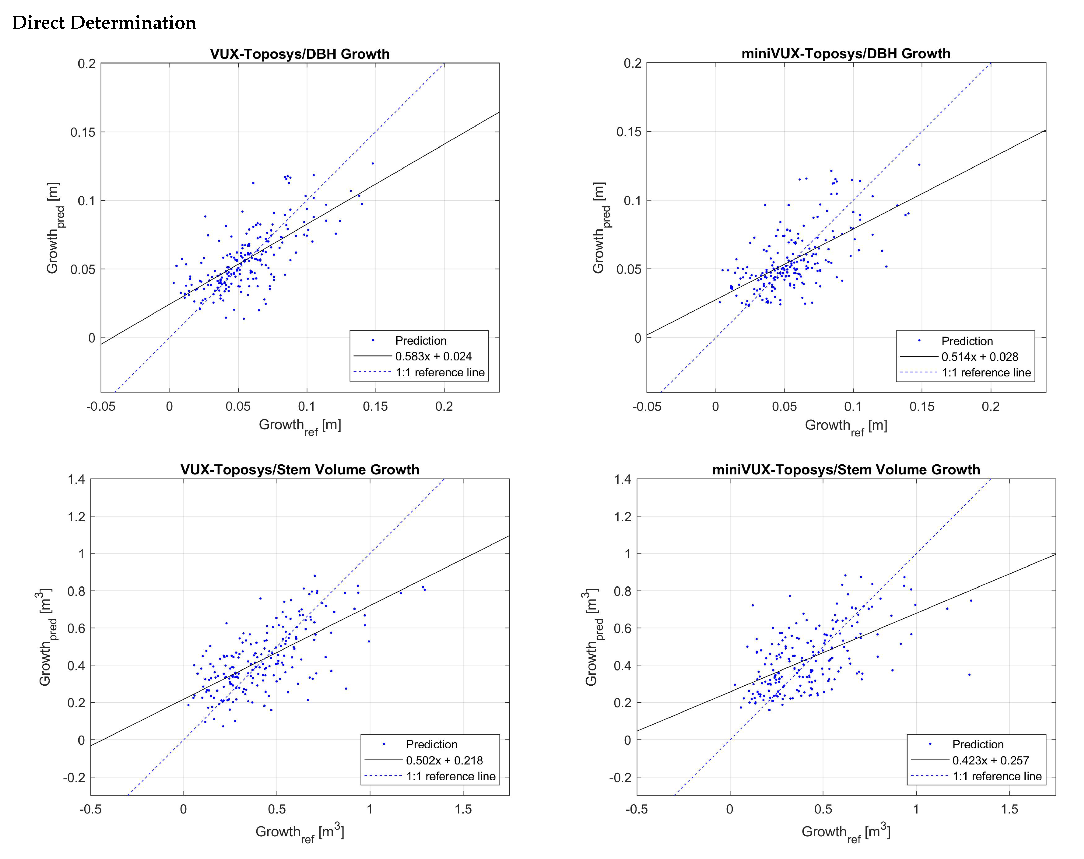
The results show that the direct method is better than the indirect method for predicting the growth value according to most of the metrics, except for the best-fit slope values and the bias value of the miniVUX-Toposys stem volume growth determination, both of which have favourable values on the indirect determination side. In the direct growth determination, the denser VUX data seem to produce better results than the sparser miniVUX data. In the indirect determination, the values obtained from VUX-Toposys data seem better in most cases, but the stem volume growth determination seems better when determined with miniVUX data, which may not be a general result. Of all the predicted attributes, the direct determination of growth from the VUX-Toposys data seems to fare best. The accuracy of height growth determination significantly outperforms the accuracy of random-forest-predicted growth values for DBH and stem volume. After all, it is the sole value that can be determined directly from the data. In its determination, the use of dense VUX data produces the best results.

In the mean growth determination in Figure 8, the averaging process fades the under- and overestimation of growth values, which is due to bias in direct growth determination or noise in indirect growth determination. However, as the graphs show, a low number of values upon which the mean is calculated can lead to a deviation from the real value. An example of this is in the miniVUX-Toposys DBH mean growth determination, where there is one sample in the category of 0.5–0.55 m. The predicted indirect growth value is roughly eight times lower than the reference value. The values of mean height growth determination do not suffer from this, as the individual predictions are much more accurate.

The tree finding (and linking) percentage illustrated in Figure 3 was limited by the raster-based tree-finding method, and the trend not to find the suppressed trees under the dominating tree layer is noticeable. This problem has already been described in previous studies [29,34,36]. In the studies by Yu et al. [29], Maltamo et al. [34], the comparable finding percentages were 69% and 40%, although in the former, the test site location was different, and the species distribution contained more pines growing in sparser groups. The latter study was conducted at the Kalkkinen test site. In this study, the 6–7 percentage point increase in the finding percentage from Toposys to miniVUX or VUX is probably explained by the shift in height distribution towards taller trees. As Figure 1 shows, the shape of the tree and its trunk and crown are better visible in the denser 2021 data. This may enable the detection of trees and measurement of their characteristics directly from the point clouds. A recent paper by Hyyppä et al. [37] may provide a way to directly measure stem curves from airborne point clouds, and its bitemporal use may result in stem volume change.

It must also be noted that another limiting factor of tree finding is the rate of linking, as the panels in Figure 3 show the results only after linking the ALS-derived trees to field-measured ones. The rather strict 2-m-$xyz$ threshold rejects some of the proposed pairs not only because of the errors in the ALS coordinates but in the field-measured coordinates. Ref. Wang et al. [38] notes that tree height, especially in taller trees, is difficult to capture accurately in field reference campaigns. The errors in the heights of the field-measured trees contribute to the low linking rates.

The CTP value combines the effect of tree finding and ALS-field-measured tree linking. The value would also benefit from better tree identification and linking rate and accuracy. The values of 71.5% and 70.9%, which are close to 30 percentage points short of 100%, further indicate that either tree finding or linking should be improved.

While it is impossible to record the correctness of ALS–field reference linking without manually checking all the links, it was assumed that the 2 m threshold in the $xyz$ distance filtered out most of the false ALS–field-measured coordinate pairs. The inclusion of the z coordinate is important here, as it filters out those trees whose height is inaccurately determined. As is seen in Figure 4 and Figure 5, the height is usually the most important feature in growth determination, and measuring it incorrectly would lead to the degraded performance of the random forest algorithm by simply introducing a bad-quality variable or increasing the rate of false links between ALS and field-measured coordinates. An easier task was to record the correctness of the linking between the data sets, which was done with the aid of tree IDs. As this linking only used the $xy$ distance as a threshold, the ratio of false links to all links is probably higher than with a threshold of the $xyz$ distance. As the results in Table 5 indicate, the difference in the linking favours the denser VUX data, but with a small marginal of nine more links in ALS–field reference linking and three more links between the data sets. Not all these links might be correct, and indeed, all the additional links come from false links in the linking between the data sets.

The feature importance distributions in Figure 4 and Figure 5 show that in direct growth determination, none of the features reaches such importance as the most important features in indirect growth determination. This is partly because the point clouds differ in densities, meaning the differences in the features derived from the data may not be correlated very well with the growth of any of the attributes. In indirect growth determination, the predictions are made for each set of ALS data separately, and the problem of differing point clouds is therefore circumvented. In future studies, it may be worth only using such features that can be measured with a similar accuracy from point clouds of different years if a direct determination is to be made.

A new discovery with the indirect growth determination is that with high-density point clouds, it is worth deriving some new features directly from the point cloud. This is seen with the variable normalizedHits (Table 4). Although the feature is normalised with the number of points per whole plot, so it should be the same in the sparse and dense data, it may be that the more accurate tree image created by the points in the dense data is better correlated with the tree attributes than in the sparse data. The variable maxDens also has a larger importance score with the denser data, but this is to be expected, as the value is associated with the points from the stem, which are mostly missing from the older and sparser data.

The filter described in Section 2.4.3 had some positive effects on the results of indirect growth determination. As Figure 7 shows, most of the outlier values are quite distant from the 1:1 reference line. In contrast, not all the outlier values or the worst outliers are captured, and notably, some inlaying values are falsely marked as outliers. It must be noted that the use of a stricter standard deviation limit of less than 2.5 would have captured more of the outlying values, but more false inlaying values could also have been marked as outliers. In height growth determination, the filter did not mark any values as outliers. This is because the filter compared height growth to height growth, creating a 1:1 line, and the height growth values were sufficiently dense to fit between the 2.5 standard deviation range.

It was noted that the filter did not work with direct growth determination, as it clearly marked inlaying points as outliers, and the filter was therefore not used. This behaviour was possible because values the filter considered as outliers could really have grown substantially more or less than other values in the 25-sample moving window. If the random forest algorithm then managed to predict their growth correctly, a mismatch occurred, and an inlaying value was marked as an outlier. The reason the filter worked better with indirect determination is probably because the outliers in indirect growth determination are more pronounced, which can be seen by comparing the similar scales in Figure 6 and Figure 7. The workings of the filter could not be fully optimised because no external data set for testing the filter was used. Optimising the filter for the results by using the data used in this study would have led to overly optimistic results.

It was observed that the bias-correcting method described in Section 2.4.1 worked better when the predicted values had little noise but were significantly off the 1:1 reference line due to regression to the mean. In this case, the bias-correcting linear fit predicted the bias correctly and shifted the slope towards a value of one. In direct growth determination, the slope shifted noticeably towards one, the value it should have attained, which Table 7 shows. However, due to noise in the linear-fitting phase, the shift was insufficient to fix all the bias. Moreover, some of the RMSE values deteriorated slightly, as some of the outlying values obtained the wrong bias-fix value and were shifted further from the 1:1 reference line. However, the fix for the best-fit slope and the $R^2$ value were more valued, and the method was therefore used. For the indirect change detection, the bias-fixing method was applied for the individual attribute predictions, but the results are reported for their difference. As Table 7 shows, the effect of the bias-fixing method was positive but less than in the direct case, where the effect was more noticeable on the best-fit equation and $R^2$ values.

The study clearly shows that height, which can be directly derived from the data without any predictive models, produces the most accurate growth values. The use of the random forest algorithm clearly diminishes the accuracy of the growth values. In the future studies, where the growth of DBH and stem volume or other attributes are measured, it may therefore be advisable to derive the attributes from the data whenever possible. However, this requires the use of very high-density data, and the practicality of directly deriving the attributes should be studied further. One possibility could be to use the stem curve of the trees to determine the growth of the DBH and stem volume. The feasibility of stem curve determination from mobile laser data and airborne laser data is studied in Hyyppä et al. [39] and Hyyppä et al. [37], but the feasibility of the algorithm for growth determination, especially with sparse data, has yet to be tested.

5. Conclusions

In this paper, we demonstrated a 20-year growth analysis in a boreal forest at the individual tree level and compared both direct and indirect estimation techniques. The article shows that it is possible to determine long-term diameter and stem volume growth values of individual trees from bitemporal airborne laser scanning point cloud data with reasonable accuracy (35–39% RMSE-% for diameter and 40–45% RMSE-% for stem volume), apart from height growth, which can be obtained with high accuracy (22–25% RMSE-%). The direct method, where the diameter at breast height and stem volume growth are predicted directly from the changes in the derived features, produces better metrics ($R^2$, RMSE-% and bias) but has a worse best-fit line fitted to the predicted-versus-referenced growth values. On the other hand, the indirect method, where the tree attributes are derived separately, and the growth is determined as their difference, produces a better best-fit line but worse metrics. Both methods benefit from the bias-fixing method used in the study.

The biggest problems hindering the use of the bitemporal airborne laser scanning data for reporting tree level changes include the detection of the individual trees from the point clouds, their related linking or registration problems, and the largely varying data and forest characteristics in the study. Both problems may be solvable by using denser point clouds, using more accurate tools for field measurements, developing more advanced point-cloud-based approaches to tree identification, and developing new features describing the change.