Modeling Forest Fire Spread Using Machine Learning-Based Cellular Automata in a GIS Environment

Abstract

The quantitative simulation of forest fire spread is of great significance for designing rapid risk management approaches and implementing effective fire fighting strategies. A cellular automaton (CA) is well suited to the dynamic simulation of the spatiotemporal evolution of complex systems, and it is therefore used to model the complex process of forest fire spread. However, the process of forest fire spread is linked with a variety of mutually influencing factors, which are too complex to analyze using conventional approaches. Here, we propose a new method for modeling fire spread, namely LSSVM-CA, in which least squares support vector machines (LSSVM) is combined with a three-dimensional forest fire CA framework. In this approach, the effects of adjacent wind on the law of fire spread are considered and analyzed. The LSSVM is utilized to derive the complex state transformation rules for fire spread by training with a dataset based on actual local data. To validate the proposed model, the forest fire spread area simulated by LSSVM-CA and the actual extracted forest fire spread area were subjected to cross-comparison. The results show that LSSVM-CA performs well in simulating the spread of forest fire and determining the probability of forest fire.

1. Introduction

Forest represents a material foundation that is important for a country’s sustainable development, and it is also an important renewable resource in the construction of the economy and ecological environments [1]. Forests provide habitat for wildlife and protect biodiversity [2]. However, forest ecosystems are often subjected not only to natural disturbances but also to manmade damage, including forest diseases, pests, and forest fires [3,4,5]. Every year, millions of hectares of forests are destroyed by wildfires that seriously threaten human life and property safety [6,7]. When a forest fire is very serious, it will destroy natural ecological species and ecological structure, even threatening human safety and affecting the regional carbon cycle [8,9,10]. Suppressing wildfires to preserve life and properties has become one of the most critical tasks in preserving natural resources [11,12].

The accurate modeling of forest fire spread facilitates the rational allocation of fire prevention resources and the development of timely and effective fire suppression strategies [13]. In general, forest fire spread models can be classified into three types [14]: remote sensing, physical, and algorithmic.

Remote sensing technology can provide the necessary environmental information required to monitor and forecast fire spreading [15,16]. In remote sensing models, a GIS (geographic information system) is usually used to explore the spatial distribution pattern of forest fires [17]. GIS data have been used to analyze the spatial and temporal distribution characteristics of factors that affect forest fires in different regions [18]. It has been shown that GIS is available for constructing forest fire simulation and rescue systems in formulating corresponding fire prevention measures for local forestry bureaus [19].

Based on the continuous investigations of numerous researchers, many physical models of forest fire behavior based on complex mechanisms have been developed since the concept of forest fire spreading models first appeared in 1946 [20]. FIRETEC and WFDS (Wildland Fire Dynamics Simulator) [21], Physical Modeling of Fire Storms in Russian Federation [22], Meso-NH model in Portugal [23], and FIRESTAR in France [24,25,26] are examples of widely used physical models. Due to the harmful nature and instability of forest fires, it is difficult to obtain measurement results of parameters required by some models under uncontrolled conditions. Thus, if a physical model relies on large-scale environmental data, its computational cost and complexity would make infeasible for practical use [27].

There are also empirical models and semi-empirical models that have been developed from physical and empirical models, and these are mainly based on the statistical analysis of existing real data events [28,29,30,31]. American scholars put forward the Rothermel model in 1972 through field and laboratory experiments combined with the energy conservation law [32]. The Rothermel model has a total of 11 test parameters, which are used to predict the speed and intensity of fire spread. Although it has a complex model structure and requires a large input, it is still widely used model in fire simulation [33]. With the development of model research, empirical models including McArthur model [34] and CFRRS (Canadian Fire Risk Rating System) [35] were proposed and are now widely used. Although the calculation and implementation of this kind of model are simple, a large number of long-term data measurements are required, and the accuracy of these measurements is highly dependent on the data and may be easy affected by measurement factors.

Recently, the application of algorithmic models is becoming increasingly widespread in the field of forest fire prediction [36,37]. For example, the ARMA (autoregressive moving average) model was used to predict and simulate the damage area of forest fires, and it was found that forest fires exhibit an outbreak cycle in China [38]. Using forest fire data in the Daxinganling region from 1990 to 2009 and based on the principle of SVM (support vector machine), a forest fire risk prediction model was derived for local forestry departments to develop fire prevention strategies [39]. Least squares support vector machines is an improved method based on SVM for forest fire prediction using historical forest fire data [40]. Bayesian network has also been used to model and predict the possible causes of forest fires and analyze the interactions between these possible causes [41,42,43]. Use of a model with a self-learning scheme was shown to have higher accuracy than the model without this scheme [44,45,46,47]. In addition, the continuous development of fire spread models [48] since the 1970s has facilitated the emergence and application of fire growth simulation software, such as Prometheus and Farsite [49,50], which are important fire management tools for predicting future fire boundaries and associated fire spread behavior.

Cellular automata are well suited to the dynamic simulation of the spatiotemporal evolution of complex systems and have also been applied to reproduce the evolution of natural phenomena, such as the spread of epidemics [51,52] and in ecological [53,54,55] and urban growth [56,57] modeling.

In physical models, cellular automata are an idealized physical system model that is discrete, not only in time but also in space and whose physical parameters only take numerical sets.

Cellular automata were first used to develop a suitable model for large-scale parallel computation [58]. Then, they were used in the simulation of forest fires, as they allow modeling of more complicated forest fire spread mechanisms without the need for an in-depth preliminary study of their general evolutionary causes. As a bottom-up modeling method, cellular automata can simulate the spatiotemporal dynamics of spatially complex systems by simply establishing basic transformation rules between neighboring local cells [28,59] based on the ideal heat transfer law between burning and non-burning adjacent cells under the same conditions [60]. Moreover, the model has been improved by extending the conversion rule to different cases such that it can obtain different burning probabilities for top and surface fires [61].

In most studies, optimization of the local state transition rule is one of the key research issues in the simulation of fire spread [62]. The traditional local transition rule for square lattice CA models was updated [63] and then extended for hexagonal dot-matrix CA modeling [64].

Considering a regular grid and constant wind direction may lead to fire spread along the axis of the grid rather than the real direction of the wind, leading to the proposal of a cell-based simulator with an irregular grid [65] to allow the modeled shape of fire spread to be closer to that of the real observed elongated fire shape. In addition, the neighborhood of each unit can be extended beyond the neighboring units such that there are more choices for flame propagation direction [66]. Due to the spatial inhomogeneous combustion process of fuel, a hexagonal model of fuel cell network propagation is proposed to predict inhomogeneous fire behavior [67].

In addition, the local transition rule was developed for the CA modeling approach, which takes into account differences in fire spread variability between the same and different materials [68]. In order to alter the linear frontier for the local transfer rule, the cyclic spread of fire fronts from diagonal units was applied [69]. Later, based on a physical modeling approach, the meta-automata rules from vegetation and flame features were defined [70]. In addition, with the development of CA models, a new model based on satellite images at the macroscale and using multi-scale 3D CA to simulate fires was proposed [71], which emphasizes the ability of CA to solve spatial heterogeneity and other aspects. In another way, the effects of fire suppression strategies, fire burn probabilities, and burn processes or fire physical velocity models were incorporated into the transition rules so that the basic CA model [72,73,74] could be more practical in modeling the spread of fine-scale mountain fires [62,72,75].

Currently, a new algorithmic model combined with a physical model that uses an extreme learning machine (ELM) instead of traditional transformation rules was proposed, named ELM-CA [59], in which data gathered from fires in western USA were used to validate the performance of the model. However, the extreme learning machine is used to solve matrix pseudo-inverses and is only applicable to single hidden layer neural networks. It is prone to overtraining, which results in degradation of the generalization performance.

Research has shown that forest fire spread is a complex process related to a variety of factors. The factors that mainly influence forest fire spread are the combustible material factor, meteorological factor, and topographic factor, which are too complex to analyze using conventional approaches and require the simulation of parallel processing, heuristics, and intelligent thought processes [59,62,76].

In this paper, we propose a machine learning-based forest fire spread model in which the traditional cellular automata framework is combined with LSSVM (least squares support vector machines). In this modeling approach, the effects of adjacent wind on the law of fire spread are considered and analyzed. The proposed model utilizes LSSVM to derive the non-linear transformation rules for fire burning probabilities for the cellular automata. This simplifies the requirement for a physical interaction process and complex heat transfer law evaluation of the evolutionary rules for fire spread. The forest fire spread area simulated using LSSVM-CA and the actual extracted forest fire spread area are subjected to cross-comparison. The results show that the proposed model performs well in simulating the spread of forest fires and determining the probability of forest fire occurrence.

The rest of this article is structured as follows. Section 2 presents the process of modeling the proposed machine learning-based cellular automata by explaining the basic principle and the methods used for modeling. Section 3 presents data processing of the study area and the simulation results and analysis. Section 4 discusses the findings. Section 5 concludes the paper and present avenues for future work.

2. Model Development

The flowchart of the proposed method is shown in Figure 1. First, we used the AETER GDEM 30 m × 30 m resolution digital elevation data and Landsat8 data to extract the driving influence factor data and fire point data. With these data, LSSVM was trained to derive the non-linear rule for the probability of fire burning. Meanwhile, the probability of the influence of meteorological factors on the adjacent CA raster was analyzed and combined into the CA model to simulate forest fire spread. In order to validate the proposed model, the burned area of a historical fire was derived using Sentinel 2 data and used to conduct cross-comparison between the actual burned area with the simulated burned area [59,77].

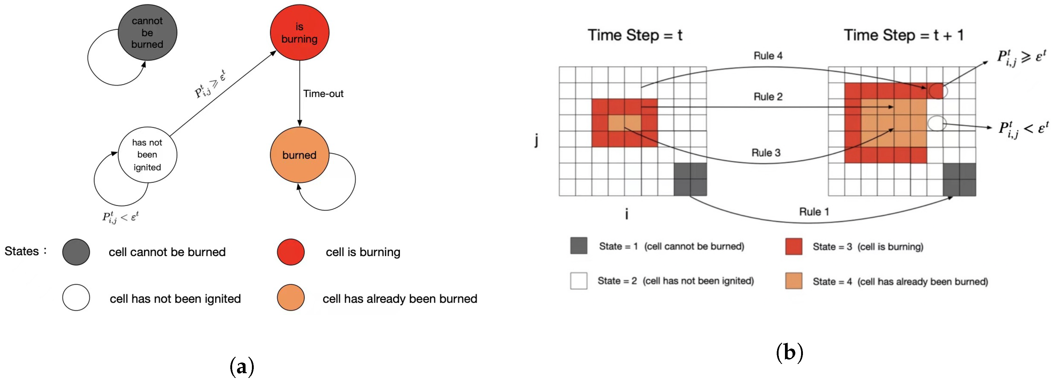
2.1. Principle of Cellular Automata

The square lattice cell is widely used as the cell of the CA framework, as it can simplify the computation and significantly reduce computational complexity [59]. Moore-type criterion is used as the criterion for classifying the neighborhood of a two-dimensional cell. The square grid cell can be divided into four possible states at different discrete time steps: cannot be burned, has not been ignited, burning, and has been burned (see Figure 2).

In a meta-cellular automaton system, the state of each cell evolves in discrete time steps depending on a finite set of state transfer rules. Figure 2a indicates the types of events that lead to each state transition at the next discrete time step $(t+1)$; the possible transitions of a cell, $A(i,j)$, are as follows:

• If the cell cannot be burned due to lack of fuel, then it remains in the same state at the next discrete time step.
• If the cell is burning, its state is updated to burned at the next discrete time step.
• If the cell is burned, then it remains in the same state at the next discrete time step.
• If the cell has not been ignited and at least one its neighboring cells is burning $A(i\pm 1,j\pm 1)$, and if the state transition likelihood $P_{i,j}^t$ of the cell $A(i,j)$ is higher than a random probability threshold ${ϵ}^t$, then its state is updated to burning at the next discrete time step.

The random probability threshold in Equation (1) is calculated using the following formula [59,76]:

$${ϵ}^t=\beta \times 1/(1+{(-ln{\gamma }^t)}^{\alpha }$$

(1)

where $\alpha$ and $\beta$ are constant values, $\gamma$ is a random number between 0 and 1.

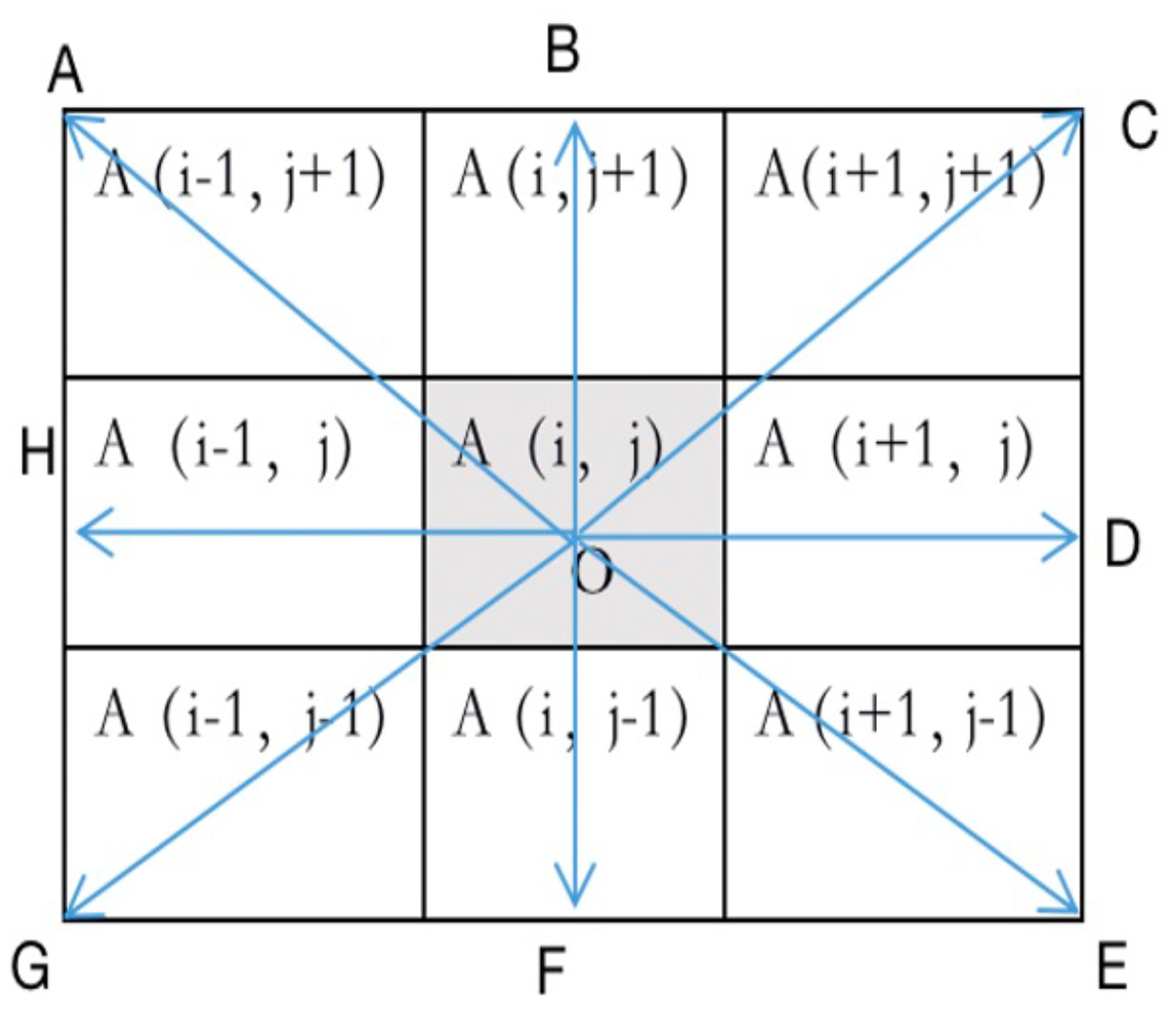
2.2. Adjacent Wind Effect

In fire spread modeling, wind is widely recognized as an essential factor affecting the velocity and direction of fire spread. Based on the equation of the influence of wind, the coefficient of wind action ($K_w$), and wind velocity (V) can be expressed as [74].

$$K_w=e^{0.1783V}$$

(2)

Due to the varying impact of wind on the spread of fire, it is necessary to derive the wind effect on the eight surrounding neighbor cells, as shown in Figure 3.

Assuming that the wind direction is counterclockwise rotated to $\overrightarrow{OB}$ with an angle of $\theta$, the projection of the wind blowing in the direction of $\overrightarrow{OB}$ is $Vcos\theta$. Similarly, the projection components of the wind direction, V, in any direction can be derived. With this and Equation (2), the wind direction coefficients for the eight directions can be expressed as $\overrightarrow{OA}:e^{0.1783Vcos(315-\theta )}$, $\overrightarrow{OB}:e^{0.1783Vcos\theta }$, $\overrightarrow{OC}:e^{0.1783Vcos(\theta -45)}$, $\overrightarrow{OD}:e^{0.1783Vcos(\theta -90)}$, $\overrightarrow{OE}:e^{0.1783Vcos(\theta -135)}$, $\overrightarrow{OF}:e^{0.1783Vcos(\theta -180)}$, $\overrightarrow{OG}:e^{0.1783Vcos(225-\theta )}$, $\overrightarrow{OH}:e^{0.1783Vcos(\theta +90)}$, respectively [74]. Then, the neighboring wind effect $\theta {(i,j)}_t$ can be calculated using Equation (3).

$$\theta {(i,j)}_t=\frac{{\sum }_{i=0}^n{\sum }_{j=0}^n{K}_w\times c(i,j)}{{\sum }_{i=0}^n{\sum }_{j=0}^n{K}_w}$$

(3)

where $c(i,j)$ indicates the cell is burning or not. If the cell is burning, it is 1. Otherwise, it is 0.

2.3. Igniting Probabilities

The classical application area of LSSVM is classification, so it is often used as a classifier. Here, we consider the change of a cell in cellular automaton from one state to another as a classification problem. When studying the spread of forest fires, the main concern is whether the current cell state can be converted to a burning state; if so, then the cell is a fire point at the next moment and is recorded as 1, otherwise the cell is not a fire point at the next moment and is recorded as 0. Therefore, the transition space of the cell is $\{0,1\}$, and the conditions for this transition and non-transition are mainly due to the current factors that can affect the cell’s state. Therefore, the influence factor of the cell itself can be recorded as the sample space such that the determination of forest fire spread using the cellular automata transformation rule can be considered a classification problem. That is, the cell transformation value can be judged according to the conditions.

Given a training set of N samples, where the ith input data are $x_i\in R^n$ and the corresponding ith output data are $y_i\in \{0,1\}$, the goal of a categorical support vector machine is to construct a classifier of the following form:

$$f\left(x\right)=sign\left[{\omega }^{\top }\phi \left(x\right)+b\right]$$

(4)

The least squares support vector classification problem is ultimately the optimization problem of solving Equation (5) as follows

$$\underset{\omega ,e}{min}(\omega ,e)=\frac{1}{2}{\omega }^{\top }\omega +\gamma \sum _{i=1}^N{e}_i^2$$

(5)

and satisfying the equation constraint.

$$y_i\left[{\omega }^{\top }\phi \left(x\right)+b\right]=1-e_i,i=1,2,\dots ,N.$$

(6)

The Lagrangian polynomial for the dual problem of Equation (6) is

$$\begin{array}{c}L(\omega ,b,e,a)=J(\omega ,e)-\sum _{i=1}^N{a}_i\left\{y_i\left[{\omega }^{\top }\phi \left(x\right)+b\right]-\left(1-e_i\right)\right\}\hfill \end{array}$$

(7)

where $a_i$ is the Lagrange multiplier, which can be positive or negative due to the equation constraint. The optimality condition is that the partial derivatives are all 0, i.e., Equation (8).

$$\left[\begin{array}{cccc}I& 0& 0& -Z^T\\ 0& 0& 0& -y^T\\ 0& 0& \lambda I& -I\\ Z& y& I& 0\end{array}\right]\left|\begin{array}{c}\omega \\ b\\ e\\ \alpha \end{array}\right|=\left|\begin{array}{c}0\\ 0\\ 0\\ \overrightarrow{1}\end{array}\right|$$

(8)

In order to eliminate e and $\omega$, the Mercer condition will be used here, i.e., Equation (9).

$$\begin{array}{c}{\Omega }_{kj}=y_k{y}_j\phi {\left(x_k\right)}^{\top }\phi \left(x_j\right)=y_k{y}_{j}K\left(x_k,x_j\right),k=1,2,\dots ,N\hfill \end{array}$$

(9)

The system of equations obtained is related to b, $\alpha$. Using the above conditions the system of equations is transformed into Equation (10).

$$\left[\begin{array}{cc}0& {-y}^T\\ y& \Omega +{\gamma }^{-1}I\end{array}\right]\left|\begin{array}{c}b\\ \alpha \end{array}\right|=\left|\begin{array}{c}0\\ \overrightarrow{1}\end{array}\right|$$

(10)

Assume $A=\Omega +{\gamma }^{-1}I$. Where A is a symmetric semi-positive definite matrix, therefore its inverse matrix $A^{-1}$ exists. Ultimately, the LSSVM classifier can be expressed as Equation (11).

$$\overline{y}\left(x\right)=sign\left[\sum _{i=1}^N{\alpha }_i{y}_{i}K\left(x,x_i\right)\right]+b$$

(11)

Here, the classification decision function $f\left(x\right)={\sum }_{i=1}^N{\alpha }_i{y}_{i}K\left(x,x_i\right)+b$ can be softened to a hard classification by a logistic transformation of the plane, and the probability of each cell being converted to a fire point can then be calculated as Equation (12).

$$P_c=\frac{1}{1+e^{-\left({\sum }_{i=1}^N{\alpha }_i{y}_{i}K\left(x,x_i\right)+b\right)}}$$

(12)

where $x_i$ is the support vector, $y_i$ is the y value corresponding to $x_i$, $P_c$ is the probability that the fire influence factor affects the cell transition, ${\alpha }_i$ is the Lagrangian coefficient of the $x_i$ object, and $K\left(x,x_i\right)$ is the kernel function. Here, a kernel function with a strong localization, such as the Gaussian radial basis kernel function is chosen, i.e., $K(x,x_i)=e^{{-\left|\right|x_k-x_i\left|\right|}^{\frac{1}{2{\sigma }^2}}}$, Then Equation (12) can be rewritten as Equation (13).

$$P_c=\frac{1}{1+e^{-\left({\Sigma }_{i=1}^N{\alpha }_i{y}_i{e}^{-\frac{1}{2{\sigma }^2}{∥x_k-x_i∥}^2}+b\right)}}$$

(13)

where $x_k$ is the vector corresponding to the kth cell, $a_i$ is the Lagrangian coefficient of the $x_i$ object, $x_i$ is the support vector, $y_i$ is the y-value corresponding to $x_i$, the decision function penalty parameter is c, and the radial basis function coefficients $\sigma$ are selected by a combination of comparisons, with $c=1$ and $\sigma =1$. Then, Equation (13) can be rewritten as Equation (14).

$$P_c=\frac{1}{1+e^{-\left({\Sigma }_{i=1}^N{\alpha }_i{y}_i{e}^{-\frac{1}{2}{∥x_k-x_i∥}^2}+b\right)}}$$

(14)

However, the use of meta-cellular automata for modeling forest fires cannot be simply regarded as a classification problem. The various interactions within the meta-cellular neighborhood and the influence of adjacent wind effects must also be considered.

According to the work of GA Trunfio [59,63], cell transition functions can be affected by two parts: internal transfer and local interactions. For each cell $A(i,j)$ in this study, the cell state transfer probability can also be expressed as a function of two subcomponents, as shown in Equation (15).

$$P_{(i,j)}^t=p{(i,j)}_t\times \theta {(i,j)}_t$$

(15)

where $p{(i,j)}_t$ is the ignition probability (Equation (13)), which is used to measure the ignition probability of the cell affected by its own factors, and $\theta {(i,j)}_t$ represents the adjacent wind effect on this cell. Hence, the formula can be changed to Equation (16):

$$P_{(i,j)}^t=\frac{1}{1+e^{-\left({\Sigma }_{i=1}^N{\alpha }_i{y}_i{e}^{-\frac{1}{2}{∥x_k-x_i∥}^2}+b\right)}}\times \frac{{\sum }_{i=0}^n{\sum }_{j=0}^n{K}_w^{\star }c(i,j)}{{\sum }_{i=0}^n{\sum }_{j=0}^n{K}_w}$$

(16)

2.4. Spreading Time Step

Another key element for forest fires is the time step, which influences the spatial distribution characteristics of forest fire spread. The time step (t) is calculated using the following Equation (17).

$$t=\frac{L}{R}$$

(17)

where L is the centroid distance between two adjacent cells. R is the rate of fire spread considering the spatial fuel distribution and influence of wind and terrain slope, which is evaluated multiplying the initial fire spread speed by the fuel spatial distribution and arrangement adjusted index, by the wind speed adjusted index ($Kw$), and by the slope adjusted index ($K\varphi$) [74,78,79].

$$K_{\varphi }=e^{3.533{\left(tan\varphi \right)}^{1.2}}$$

(18)

where $\varphi$ is the terrain slope angle.

With this, the rise of the fire front isometrics can be simulated with the iteration at each time step throughout the burning process. The continuous time of the fire spreading process can be converted into a discrete-time state using the time step such that the states of fire can be updated during the fire propagate process at each time step.

3. Case Studies

3.1. Study Area and Data

The historical fire data of the Lushan area of Liangshan Prefecture, Sichuan Province, were collected for use in verifying the proposed model (Figure 4). A point source ignition is used in this scenario—which was investigated and recognized as the actual forest fire starting point—that broke out in this area at 15:35 on 30 March 2020 just before the major fire spread event started, causing a total area of 3047.7805 hectares of various types of burned land, and 791.6 hectares of fire-affected forest area [80]. Lushan Mountain is 2317 m above sea-level, bordered by Qionghai Sea in the east, Anning River to the west, the ancient city of Xichang to the north, and the Luoji Mountain to the south. The wind power on the day of the fire reached 7–8 [80]. Using ArcGIS tools, the influencing factors, slope, direction, elevation, NDVI, and relative humidity were obtained from the remote sensing data for the area.

First, the dependent variable data (fire point) and independent variable data (slope, aspect, elevation, relative humidity, normalized vegetation index) of Xichang and Lushan areas were obtained, and then 30% of Xichang data were screened through spss and 70% of the Lushan data were used as training data for the least squares support vector machine. Then, the least squares support vector machine was used for classification processing, and after training using 25,133 sample points, 25,133 support vectors were obtained, and with b = −0.9512 and Equation (14), the final fire impact probability expression can be determined as Equation (19).

$$P_c=\frac{1}{1+e^{-\left({\Sigma }_{i=1}^N{\alpha }_i{y}_i{e}^{-\frac{1}{2}{∥x_k-x_i∥}^2}-0.9512\right)}}$$

(19)

The final fire ignition probability can be obtained by using Equation (13) and the adjacent wind effect. Then, the cellular automata can be used to simulate the spreading of fire.

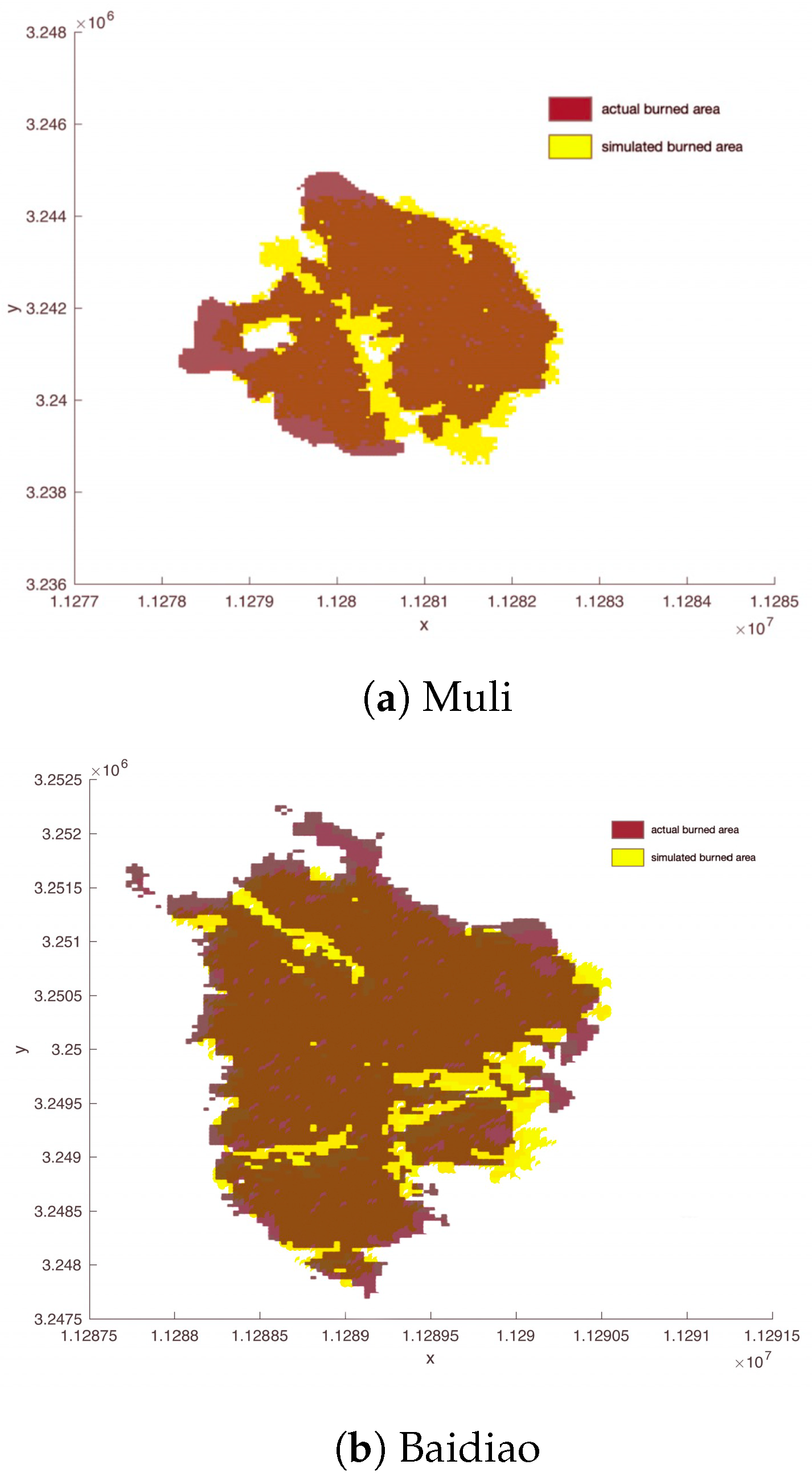
3.2. Simulation Results and Analysis

Figure 5 shows the simulation of the fire spreading process from the initial fire point to the end every 5 h. For each model, the simulated fire spread direction is basically in line with the actual fire spread direction of official reports [80]. From Figure 5, it can be found that the fire spread rate in the northeast direction is faster than that in the southwest direction due to the influence of wind. However, there is dense vegetation in the southwest direction, where there are burning conditions. Although the southwest direction is not downwind, there is also a tendency for fire spreading in this direction. The proposed method and the basic CA simulation of fire spread and the actual spread direction are shown in Figure 5b,c, respectively. Finally, the simulated burned area of the forest fire can be obtained. Comparing the simulated burned area with the actual burned area (Figure 6), the difference between the simulated forest fire area and the actual area can be seen more clearly, as shown in Figure 7.

In order to more accurately simulate and observe the trend of forest fire spread, it is necessary to evaluate the spatial accuracy of the results of the spread model. In forest fires, the burned area is important for evaluating the fire size, estimating the loss of stockpile, and calculating the economic loss due to the fire. Equations (20)–(22) are commonly used to evaluate the space accuracy of the fire spreading model [81].

$$\mu =\frac{S_1\cap S_2}{S_2}\times 100\%$$

(20)

$${\epsilon }_1=\frac{S_2-(S_1\cap S_2)}{S_2}\times 100\%$$

(21)

where $S_1$ is the simulated burned area, and $S_2$ is the actual fire area. $\mu$ is the ratio of the area where there is overlap between the simulated burned area and the actual fire area to the actual fire area. ${\epsilon }_1$ is the ratio of the actual fire area that is not predicted to the actual fire area. $\mu$ and ${\epsilon }_1$ describe the degree of intersection between the simulated and the actual fire area.

$${\epsilon }_2=\frac{S_1-(S_1\cap S_2)}{S_2}\times 100\%$$

(22)

${\epsilon }_2$ is the ratio of the simulated burned area that was not actually burned to the actual fire area. It describes the deviation between the simulated burned area and the actual fire in spatial terms.

The actual fire area is 33,735 grids (Figure 6). In terms of the burned area in Figure 5, as shown in

Table 1. Comparison between the actual and simulated results.

State	LSSVM-CA	ELM-CA	CA
$\mu$	33,028 (97.9%)	30,602 (90.71%)	29,634 (87.84%)
${\epsilon }_1$	707 (2.1%)	3133 (9.29%)	4101 (12.16%)
${\epsilon }_2$	3083 (9.14%)	3191 (9.46%)	4091 (12.13%)
$S2$	33,735
$S1$	36,111	33,793	33,725

, the number of burned grids simulated by LSSVM is 36,111 grids. The number of simulated burned grids is 33,793 and 33,725 grids in ELM-CA and the basic CA model, respectively. From Table 1, we can see that the simulated burned area determined using the three models mostly coincides with the actual fire area. Compared with the other methods, the proposed method demonstrates lower deviation between the simulated burned area and the actual fire in spatial terms.

In order to further evaluate the performance of the model, two other forest fires that occurred in Liangshan Prefecture, Sichuan Province, were simulated. In recent years, fires have frequently occurred in Liangshan Prefecture. The Muli fire was the first fire subjected to simulation. It occurred on 28 March 2020 at the junction of Qiaowa Town and Xiangjiao Village in Muli County. The fire was caused by human carelessness. The wind on the day of the fire was in the northwest direction and reached 2.7 m/s.

The second fire subjected to simulation was the fire near Baidiao country, which occurred on 3 April 2020. Most of the area is high mountains that are low in the south and high in the north, near the Yalong river. The wind on the day of the fire was in a southwest direction and was about 1.5 m/s.

Figure 8 shows the simulation of the initial spreading process of the Muli and Baidiao fires. For each fire, the simulated fire growth is basically in line with the spread direction of the actual fires. From

Table 2. The results of simulated Muli and Baidiao fires.

State	Muli	Baidiao
$\mu$	4091 (83.85%)	5408 (85.0%)
${\epsilon }_1$	788 (16.15%)	957 (15.0%)
${\epsilon }_2$	787 (16.13%)	350 (5.5%)
$S2$	4879	6365
$S1$	4878	5758

, we can see burned areas simulated by the model basically coincide with the majority of the actual fire area (Figure 9). The results of the proposed method show good spatial accuracy between the simulated burned area and the actual fire.

4. Discussion

The spread of forest fire contains inherent uncertainties due to the diversity in combustible material and the complexity of the geographic environment. It is not easy to obtain the exact parameters of various combustible material characteristics of the whole forest area or to apply localized fuel behaviors to the whole area [64,69].

Machine learning-based CA models are attractive for application in simulating forest fire spread as they allow spatiotemporal modeling of the complicated spread mechanisms without the need for an in-depth preliminary study of their general evolutionary causes [63,82]. With the increase in computerized modeling, CA have been commonly used to simulate fire spread as discrete processes on a regular spaced cell [62,68,69]. Although good simulation performance was obtained in the LSSVM-CA model, it is not without limitations.

In a fire, the combustion material in the burning cell may affect the surrounding non-adjacent cells in an unintended way [83]. For example, the burning material may fly into and ignite the non-adjacent cells due to blowing wind. This phenomenon could cause underestimation of the real fire spreading speed in proposed models [82,84,85].

The state of a cell is affected by transition rules and the state of its adjacent cells [86]. When a central cell has multiple adjacent burning cells to which the fire spreads at the same time, the contribution to its state transition may be underestimated. Consequently, this will impact the model effectiveness [85].

It is not easy to compare the performance of one model with another when different fire characteristics and fuel are employed or different kinds of transition rules (such as stochastic and deterministic) are used. However, some general observations of CA-based methods can be obtained on the basis of the transition rules [82].

In [85], the state weight coefficient of a burned cell was introduced to account for the overlapping of the burning areas, then an empirical fire spread model was used. However, the use of a wind coefficient resulted in simplification of the effect of the adjacent wind.

Due to the complexity of the forest environment, the factors and parameters involved in modeling of a specific forest environment may not be available in other places. Thus, a model designed for a specific local area may not be universal and, thus, cannot be directly applied elsewhere [86]. In this model, we adopted widely used factors, such as terrain, climate, and vegetation for modeling, measure of which are obtainable through publicly available data. This makes the modeling method more applicable.

Forest fire is a multistage phenomenon taking into account inert heating, drying, pyrolysis, ignition, flame combustion, and coke after burning. The behavior at the fire front is mainly dependent on the fire properties of the fuel; however, some dynamic inputs and factors may not be directly obtained in CA [87,88]. For instance, in order to select the available model, up to 15 kinds of the rate of fire spread models are trained to select the most appropriate model based on a burning experiment [89].

Considering the uncertainties, empirical/statistical and physical/theoretical models are helpful for analyzing and simulating fire behavior [90]. Thus, CA modeling is required to adopt some equations of the fire behavior models to adapt this dynamic process [87,91,92]. To do so, statistical models and theoretical models are commonly integrated into the CA framework. However, some models require numerous primary inputs involving many factors. This may reduce their applicability.

5. Conclusions

In this paper, a new fire spread modeling method, LSSVM-CA, is proposed, in which the basic framework of traditional forest fire CA is combined with LSSVM classification. Moreover, the proposed method was validated based on historical fire data in the Lushan area of Xichang City, Liangshan Prefecture, Sichuan Province. The results show that using the least squares support vector machine model, the forest fire ignition probability formula can be effectively derived. The proposed modeling method demonstrated good performance in accurately simulating fire spread. Although the proposed LSSVM-CA model achieved relatively good performance, there are some issues to be considered in future work.

Vegetation is widely regarded as the fuel of a fire. Among all the factors (such as terrain, climate, etc.), that are used for fire spread simulation, vegetation information thus plays an important role in fire spread. With the developments in measurement technology, airborne light detection and ranging data could be used to derive and map forest attributes, such as vegetation type, density, and volume. Such forest attributes could be used as input factors to improve model performance.

Due to the historically frequent occurrence of fire in this area, it is urgent to design effective fire management strategies. In the future, we will use this model to simulate and obtain potential key fire propagation paths so as to plan efficient forest fire extinguishing strategies. These strategies include optimizing the allocation of fire-fighting resources and expanding road networks, such that the fire extinguishing capacity of the whole area can be improved at minimum cost.

Due to the complexity of fire spread, adopting and combining the most appropriate mathematical fire behavior model for a specific area into the CA modeling may improve the performance to some extent. In the future, we would investigate and try to combine CA with equations that can adequately reflect the relationships between fire behavior and the numerical values of established conditions, such as ignition risk, thermal conductivity, and flame height.

References

1. Li, Q.; Cui, J.; Jiang, W.; Jiao, Q.; Gong, L.; Zhang, J.; Shen, X. Monitoring of the fire in Muli County on 28 March 2020, based on high temporal-spatial resolution remote sensing techniques. Nat. Hazards Res. 2021, 1, 20–31. [Google Scholar] [CrossRef]
2. Kariyeva, J.; van Leeuwen, W.J.; Woodhouse, C.A. Impacts of climate gradients on the vegetation phenology of major land use types in Central Asia (1981–2008). Front. Earth Sci. 2012, 6, 206–225. [Google Scholar] [CrossRef]
3. Islam, S.; Bhuiyan, M.A.H. Sundarbans mangrove forest of Bangladesh: Causes of degradation and sustainable management options. Environ. Sustain. 2018, 1, 113–131. [Google Scholar] [CrossRef]
4. Khan, A.; Gupta, S.; Gupta, S.K. Multi-hazard disaster studies: Monitoring, detection, recovery, and management, based on emerging technologies and optimal techniques. Int. J. Disaster Risk Reduct. 2020, 47, 101642. [Google Scholar] [CrossRef]
5. Kulakowski, D.; Seidl, R.; Holeksa, J.; Kuuluvainen, T.; Nagel, T.A.; Panayotov, M.; Svoboda, M.; Thorn, S.; Vacchiano, G.; Whitlock, C.; et al. A walk on the wild side: Disturbance dynamics and the conservation and management of European mountain forest ecosystems. For. Ecol. Manag. 2017, 388, 120–131. [Google Scholar] [CrossRef] [PubMed] [Green Version]
6. Collins, B.M.; Kelly, M.; Van Wagtendonk, J.W.; Stephens, S.L. Spatial patterns of large natural fires in Sierra Nevada wilderness areas. Landsc. Ecol. 2007, 22, 545–557. [Google Scholar] [CrossRef]
7. Neary, D.G.; Robichaud, P.R.; Beyers, J.L. Burned area emergency watershed rehabilitation: Program goals, techniques, effectiveness, and future directions in the 21 century. Proc. RMRS 1998, 375, 13. [Google Scholar]
8. Sileshi, G.; Mafongoya, P. The short-term impact of forest fire on soil invertebrates in the miombo. Biodivers. Conserv. 2006, 15, 3153–3160. [Google Scholar] [CrossRef]
9. Pham, B.T.; Jaafari, A.; Avand, M.; Al-Ansari, N.; Dinh Du, T.; Yen, H.P.H.; Phong, T.V.; Nguyen, D.H.; Le, H.V.; Mafi-Gholami, D.; et al. Performance evaluation of machine learning methods for forest fire modeling and prediction. Symmetry 2020, 12, 1022. [Google Scholar] [CrossRef]
10. Matin, M.A.; Chitale, V.S.; Murthy, M.S.; Uddin, K.; Bajracharya, B.; Pradhan, S. Understanding forest fire patterns and risk in Nepal using remote sensing, geographic information system and historical fire data. Int. J. Wildland Fire 2017, 26, 276–286. [Google Scholar] [CrossRef] [Green Version]
11. Van Leeuwen, W.J. Monitoring the effects of forest restoration treatments on post-fire vegetation recovery with MODIS multitemporal data. Sensors 2008, 8, 2017–2042. [Google Scholar] [CrossRef] [PubMed]
12. Van Leeuwen, W.J.; Casady, G.M.; Neary, D.G.; Bautista, S.; Alloza, J.A.; Carmel, Y.; Wittenberg, L.; Malkinson, D.; Orr, B.J. Monitoring post-wildfire vegetation response with remotely sensed time-series data in Spain, USA and Israel. Int. J. Wildland Fire 2010, 19, 75–93. [Google Scholar] [CrossRef]
13. Zhenyang, X.; Lin, H.; Wang, F. A small target forest fire detection model based on YOLOv5 Improvement. Forests 2022, 13, 1332. [Google Scholar]
14. Li, H.; Long, Z.; Yang, Z.; Xu, Z.; Li, Y. Analysis of forest fire risk in Sichuan Liangshan based on logistic model. J. Saf. Environ. 2021, 21, 498–505. [Google Scholar]
15. Huang, Z.; Huang, X.; Fan, J.; Eichhorn, M.P.; An, F.; Chen, B.; Cao, L.; Zhu, Z.; Yun, T. Retrieval of aerodynamic parameters in rubber tree forests based on the computer simulation technique and terrestrial laser scanning data. Remote Sens. 2020, 12, 1318. [Google Scholar] [CrossRef] [Green Version]
16. Jiecheng, Z. Application of remote sensing technology in forest fire-proof technique. Inf. Agric. Sci. Technol. 2019, 8, 67–68. [Google Scholar]
17. Chu, C.C.; Zhang, G.; Sun, Y.R. Trend forecast of forest fire in Hunan province based on Kriging interpolation model. J. Cent. South Univ. For. Technol. 2014, 34, 66–70. [Google Scholar]
18. Jiachang, L.; Bin, T.; Yuan, Z. GIS-Based spatial and temporal distribution characteristics and factor analysis of forest fires—Taking California, USA as an example. J. Northeast. For. Univ. 2020, 7, 70–74. [Google Scholar]
19. Meilin, W.; Linlin, J.; Xiaohong, W.; Bin, W.; Xingxing, X. Forest fire simulation and rescue system based on Geographic Information System. Inf. Rec. Mater. 2019, 9, 144–145. [Google Scholar]
20. Fernandez-Pello, A.C. Wildland fire spot ignition by sparks and firebrands. Fire Saf. J. 2017, 91, 2–10. [Google Scholar] [CrossRef]
21. Hoffman, C.; Canfield, J.; Linn, R.; Mell, W.; Sieg, C.; Pimont, F.; Ziegler, J. Evaluating crown fire rate of spread predictions from physics-based models. Fire Technol. 2016, 52, 221–237. [Google Scholar] [CrossRef] [Green Version]
22. Grishin, A.; Golovanov, A.; Sukov, Y.V. Physical modeling of fire storms. Heat Transf. Res. 2005, 36, 517–527. [Google Scholar] [CrossRef]
23. Couto, F.T.; Iakunin, M.; Salgado, R.; Pinto, P.; Viegas, T.; Pinty, J.P. Lightning modelling for the research of forest fire ignition in Portugal. Atmos. Res. 2020, 242, 104993. [Google Scholar] [CrossRef]
24. Morvan, D. Physical phenomena and length scales governing the behaviour of wildfires: A case for physical modelling. Fire Technol. 2011, 47, 437–460. [Google Scholar] [CrossRef]
25. Balbi, J.H.; Morandini, F.; Silvani, X.; Filippi, J.B.; Rinieri, F. A physical model for wildland fires. Combust. Flame 2009, 156, 2217–2230. [Google Scholar] [CrossRef] [Green Version]
26. Frangieh, N.; Accary, G.; Morvan, D.; Méradji, S.; Bessonov, O. Wildfires front dynamics: 3D structures and intensity at small and large scales. Combust. Flame 2020, 211, 54–67. [Google Scholar] [CrossRef]
27. Cruz, M.G.; Alexander, M.E. Uncertainty associated with model predictions of surface and crown fire rates of spread. Environ. Model. Softw. 2013, 47, 16–28. [Google Scholar] [CrossRef]
28. Alexandridis, A.; Russo, L.; Vakalis, D.; Bafas, G.; Siettos, C. Wildland fire spread modelling using cellular automata: Evolution in large-scale spatially heterogeneous environments under fire suppression tactics. Int. J. Wildland Fire 2011, 20, 633–647. [Google Scholar] [CrossRef]
29. Wagner, C.V. Conditions for the start and spread of crown fire. Can. J. For. Res. 1977, 7, 23–34. [Google Scholar] [CrossRef]
30. Marsden-Smedley, J.; Catchpole, W.R. Fire behaviour modelling in Tasmanian buttongrass moorlands. II. Fire behaviour. Int. J. Wildland Fire 1995, 5, 215–228. [Google Scholar] [CrossRef]
31. Catchpole, W.; Bradstock, R.; Choate, J.; Fogarty, L.; Gellie, N.; McCarthy, G.; McCaw, W.; Marsden-Smedley, J.; Pearce, G. Cooperative development of equations for heathland fire behaviour. In Proceedings of the 3rd International Conference on Forest Fire Research and 14th Conference on Fire and Forest Meteorology, Luso, Portugal, 16–20 November 1998; Volume 2, pp. 16–20. [Google Scholar]
32. Rothermel, R.C. A Mathematical Model for Predicting Fire Spread in Wildland Fuels; INT-115; US Department of Agriculture, Forest Service, Intermountain Forest and Range Experiment Station: Ogden, UT, USA, 1972.
33. Rothermel, R. How to Predict the Spread and Intensity of Forest Fire and Range Fires; General Technical Reports, INT-143; US Department of Agriculture, Forest Service, Intermountain Forest and Range Experiment Station: Ogden, UT, USA, 1983.
34. Sullivan, A.L. Wildland surface fire spread modeling, 1990–2007. 3: Simulation and mathematical analogue models. Int. J. Wildland Fire 2009, 18, 387–403. [Google Scholar] [CrossRef] [Green Version]
35. Lee, B.; Alexander, M.; Hawkes, B.; Lynham, T.; Stocks, B.; Englefield, P. Information systems in support of wildland fire management decision making in Canada. Comput. Electron. Agric. 2002, 37, 185–198. [Google Scholar] [CrossRef]
36. Guan, Z.; Miao, X.; Mu, Y.; Sun, Q.; Ye, Q.; Gao, D. Forest fire segmentation from Aerial Imagery data Using an improved instance segmentation model. Remote Sens. 2022, 14, 3159. [Google Scholar] [CrossRef]
37. Zhang, S.; Gao, D.; Lin, H.; Sun, Q. Wildfire detection using sound spectrum analysis based on the Internet of things. Sensors 2019, 19, 5093. [Google Scholar] [CrossRef] [Green Version]
38. Dongyan, B.; Yin, Z.; Shaozhi, C.; Decheng, Z.; Youjun, H. Forest fire prediction based on Auto-Regressive Moving Average model. Pract. For. Technol. 2013, 6, 11–14. [Google Scholar]
39. Hai-yan, C.; Wei, Z.; Zhao-wen, Q. Application of SVM Model in Forest Fire Judgment. J. Anhui Agric. Sci. 2014, 42, 3684. [Google Scholar]
40. Li, E.; Fei, Y. Prediction of Forest Fires Based on Least Squares Support Vector Machine. Hans J. Data Min. 2016, 6, 15–27. [Google Scholar] [CrossRef]
41. Dawe, D.A.; Peters, V.S.; Flannigan, M.D. Post-fire regeneration of endangered limber pine (Pinus flexilis) at the northern extent of its range. For. Ecol. Manag. 2020, 457, 117725. [Google Scholar] [CrossRef]
42. Jiao, W.; Tian, M.; Xu, Y. A combining strategy of energy replenishment and data collection in wireless sensor networks. IEEE Sens. J. 2022, 22, 7411–7426. [Google Scholar] [CrossRef]
43. Jiao, W.; Tang, R.; Xu, Y. A coverage optimization algorithm for the wireless sensor network with random deployment by using an improved flower pollination algorithm. Forests 2022, 13, 1690. [Google Scholar] [CrossRef]
44. Qian, J.; Lin, H. A forest fire identification system based on weighted fusion algorithm. Forests 2022, 13, 1301. [Google Scholar] [CrossRef]
45. Lin, J.; Lin, H.; Wang, F. STPM_SAHI: A Small-Target forest fire detection model based on Swin Transformer and Slicing Aided Hyper inference. Forests 2022, 13, 1603. [Google Scholar] [CrossRef]
46. Qu, J.; Cui, X. Automatic machine learning framework for forest fire forecasting. J. Phys. Conf. Ser. 2020, 1651, 012116. [Google Scholar] [CrossRef]
47. Yang, X.; Wang, Y.; Liu, X.; Liu, Y. High-Precision Real-Time forest fire video detection using One-Class model. Forests 2022, 13, 1826. [Google Scholar] [CrossRef]
48. Kourtz, P.; Nozaki, S.; O’Regan, W.G. Forest Fires in the Computer—A Model to Predict the Perimeter Location of a Forest Fire; no. FF-X-65; Information Report Forest Fire Research Institute: Ottawa, ON, Canada, 1977. [Google Scholar]
49. Richards, G.D. The properties of elliptical wildfire growth for time dependent fuel and meteorological conditions. Combust. Sci. Technol. 1993, 95, 357–383. [Google Scholar] [CrossRef]
50. Finney, M.A. FARSITE: Fire Area Simulator—Model Development and Evaluation; USDA Forest Service, Rocky Mountain Research Station: Fort Collins, CO, USA, 1998.
51. Li, X.; Tong, B.L.; Wu, X.B. Simulation model of infectious disease transmission and control based on cellular automata. J. Liaoning Univ. Technol. Nat. Sci. Ed. 2020, 40, 290–295. [Google Scholar]
52. Ruifang, Z. Virus Propagation Control Based on Cellular Automata and Ad-Hoc Edge Deletion Optimization. Master’s Thesis, Shaanxi Normal University, Xi’an, China, 2019. [Google Scholar]
53. Yongqiang, X. The Evolution of Human-Robot Competition Based on Cellular Automata. Master’s Thesis, Nanchang University, Nanchang, China, 2018. [Google Scholar]
54. Xue, X.; Jin, S.; An, F.; Zhang, H.; Fan, J.; Eichhorn, M.P.; Jin, C.; Chen, B.; Jiang, L.; Yun, T. Shortwave radiation calculation for forest plots using airborne LiDAR data and computer graphics. Plant Phenomics 2022, 2022, 9856739. [Google Scholar] [CrossRef]
55. Sun, C.; Huang, C.; Zhang, H.; Chen, B.; An, F.; Wang, L.; Yun, T. Individual tree crown segmentation and crown width extraction from a heightmap derived from aerial laser scanning data using a deep learning framework. Front. Plant Sci. 2022, 13, 914974. [Google Scholar] [CrossRef]
56. Wang, X.Y.; Zhou, Y.; Yu, J.N. Evolution of green infrastructure layout and water-logging risk assessment based on cellular automata simulation of urban expansion: A case study of Wuhan city. Landsc. Archit. 2020, 27, 50–56. [Google Scholar]
57. Yong-jiu, F.; Miao-long, L. Modeling land use changes with machine learning-based cellular automata in a GIS environment. Sci. Surv. Mapp. 2011, 36, 216–218. [Google Scholar]
58. Li, X.; Wu, J.; Li, X. Theory of Practical Cellular Automaton; Springer: Berlin, Germany, 2018. [Google Scholar]
59. Zheng, Z.; Huang, W.; Li, S.; Zeng, Y. Forest fire spread simulating model using cellular automaton with extreme learning machine. Ecol. Model. 2017, 348, 33–43. [Google Scholar] [CrossRef] [Green Version]
60. Albinet, G.; Searby, G.; Stauffer, D. Fire propagation in a 2D random medium. J. Phys. 1986, 47, 1–7. [Google Scholar] [CrossRef]
61. Niessen, W.V.; Blumen, A. Dynamic simulation of forest fires. Can. J. For. Res. 1988, 18, 807–814. [Google Scholar] [CrossRef]
62. Bhakti, H.; Ibrahim, H.; Fristella, F.; Faisal, M. Fire spread simulation using cellular automata in forest fire. Iop Conf. Ser. Mater. Sci. Eng. 2020, 821, 012037. [Google Scholar] [CrossRef]
63. Trunfio, G.A. Predicting wildfire spreading through a hexagonal cellular automata model. In International Conference on Cellular Automata; Springer: Berlin, Germany, 2004; pp. 385–394. [Google Scholar]
64. Zhang, Y.; Feng, Z.D.; Tao, H.; Wu, L.; Li, K.; Duan, X. Simulating wildfire spreading processes in a spatially heterogeneous landscapes using an improved cellular automaton model. In Proceedings of the IGARSS 2004. 2004 IEEE International Geoscience and Remote Sensing Symposium, Anchorage, AK, USA, 20–24 September 2004; Volume 5, pp. 3371–3374. [Google Scholar]
65. Johnston, P.; Kelso, J.; Milne, G.J. Efficient simulation of wildfire spread on an irregular grid. Int. J. Wildland Fire 2008, 17, 614–627. [Google Scholar] [CrossRef]
66. Kourtz, P.H.; O’Regan, W.G. A model for a small forest fire to simulate burned and burning areas for use in a detection model. For. Sci. 1971, 17, 163–169. [Google Scholar]
67. Frandsen, W.; Andrews, P. Fire Behavior in Non-Uniform Fuels; USDA Forest Service, Intermountain Forest and Range Experiment Station: Ogden, UT, USA, 1979.
68. Karafyllidis, I.; Thanailakis, A. A model for predicting forest fire spreading using cellular automata. Ecol. Model. 1997, 99, 87–97. [Google Scholar] [CrossRef]
69. Encinas, A.H.; Encinas, L.H.; White, S.H.; del Rey, A.M.; Sánchez, G.R. Simulation of forest fire fronts using cellular automata. Adv. Eng. Softw. 2007, 38, 372–378. [Google Scholar] [CrossRef]
70. Alexandridis, A.; Vakalis, D.; Siettos, C.I.; Bafas, G.V. A cellular automata model for forest fire spread prediction: The case of the wildfire that swept through Spetses Island in 1990. Appl. Math. Comput. 2008, 204, 191–201. [Google Scholar] [CrossRef]
71. Byari, M.; Bernoussi, A.; Jellouli, O.; Ouardouz, M.; Amharref, M. Multi-scale 3D cellular automata modeling: Application to wildland fire spread. Chaos Solitons Fractals 2022, 164, 112653. [Google Scholar] [CrossRef]
72. Sun, T.; Zhang, L.; Chen, W.; Tang, X.; Qin, Q. Mountains forest fire spread simulator based on geo-cellular automaton combined with wang zhengfei velocity model. IEEE J. Sel. Top. Appl. Earth Obs. Remote Sens. 2012, 6, 1971–1987. [Google Scholar] [CrossRef]
73. Zhou, G.; Wu, Q.; Chen, A. Forestry fire spatial diffusion model based on Multi-Agent algorithm with cellular automata. J. Syst. Simul. 2018, 30, 8. [Google Scholar]
74. Yang, F.; Cao, J. Study on simulation of three dimensional simulation of forest fire spread based on cellular automation. Comput. Eng. Appl. 2016, 52, 5. [Google Scholar]
75. Wang, Z. General forest fire weather ranks system. J. Nat. Disasters 1992, 1, 39–45. [Google Scholar]
76. Pei, F.; Xia, L.I.; Liu, X.; Xia, G. Dynamic simulation of urban expansion and their effects on Net Primary Productivity: A scenario analysis of Guangdong Province in China. J. Geo-Inf. Sci. 2015, 17, 469–477. [Google Scholar]
77. Tianchi, L.; Fuqin, Y.; Yan, L. Forest fire monitoring based on Sentinel-2 image in Muli, Sichuan Province. South China For. Sci. 2020, 48, 49–53. [Google Scholar]
78. Mao, X.M.; Xu, W.X. Research on the spread speed of forest fire. J. Meteorol. Environ. 1991, 1, 9–13. [Google Scholar]
79. Zhang, Y.S. Review and prospect of researches on simulation of forest fire spread. J. Anhui Agric. Sci. 2010, 32. [Google Scholar]
80. Results of the investigation into the “3–30” forest fire in Xichang, Liangshan, Sichuan released. Firef. Community 2021, 7, 27.
81. Yufei, Z.; Pengju, L.; Xiaoming, T. Space accuracy evaluation of forest fire spreading model. J. Beijing For. Univ. 2010, 32, 21–26. [Google Scholar]
82. Yassemi, S.; Dragićević, S.; Schmidt, M. Design and implementation of an integrated GIS-based cellular automata model to characterize forest fire behaviour. Ecol. Model. 2008, 210, 71–84. [Google Scholar] [CrossRef]
83. Mutthulakshmi, K.; Wee, M.R.E.; Wong, Y.C.K.; Lai, J.W.; Koh, J.M.; Acharya, U.R.; Cheong, K.H. Simulating forest fire spread and fire-fighting using cellular automata. Chin. J. Phys. 2020, 65, 642–650. [Google Scholar] [CrossRef]
84. Freire, J.G.; DaCamara, C.C. Using cellular automata to simulate wildfire propagation and to assist in fire management. Nat. Hazards Earth Syst. Sci. 2019, 19, 169–179. [Google Scholar] [CrossRef] [Green Version]
85. Li, X.; Yang-wei, W. A forest fire spread model based on cellular automata. For. Mach. Woodwork. Equip. 2019, 47, 46–54. [Google Scholar]
86. Karafyllidis, I. Design of a dedicated parallel processor for the prediction of forest fire spreading using cellular automata and genetic algorithms. Eng. Appl. Artif. Intell. 2004, 17, 19–36. [Google Scholar] [CrossRef]
87. Domasevich, M.; Pavlova, A.; Rubtsov, S.; Telyatnikov, I. Cellular automata modeling of processes on landscape surfaces using triangulation meshes. Iop Conf. Ser. Earth Environ. Sci. 2021, 867, 012017. [Google Scholar] [CrossRef]
88. Forestry Canada Fire Danger Group. Development and Structure of the Canadian Forest Fire Behavior Prediction System; Forestry Canada, Headquarters, Fire Danger Group and Science and Sustainable Development Directorate: Ottawa, ON, Canada, 1992. [Google Scholar]
89. Currie, M.; Speer, K.; Hiers, J.; O’Brien, J.; Goodrick, S.; Quaife, B. Pixel-level statistical analyses of prescribed fire spread. Can. J. For. Res. 2019, 49, 18–26. [Google Scholar] [CrossRef]
90. Ntinas, V.G.; Moutafis, B.E.; Trunfio, G.A.; Sirakoulis, G.C. Parallel fuzzy cellular automata for data-driven simulation of wildfire spreading. J. Comput. Sci. 2017, 21, 469–485. [Google Scholar] [CrossRef]
91. Li, X.; Zhang, M.; Zhang, S.; Liu, J.; Sun, S.; Hu, T.; Sun, L. Simulating forest fire spread with cellular automation driven by a LSTM based speed model. Fire 2022, 5, 13. [Google Scholar] [CrossRef]
92. Rundle, J.B.; Turcotte, D.L.; Shcherbakov, R.; Klein, W.; Sammis, C. Statistical physics approach to understanding the multiscale dynamics of earthquake fault systems. Rev. Geophys. 2003, 41, 4. [Google Scholar] [CrossRef]
Figure 1. The flowchart of the proposed method: (a) data collection; (b) data pre-processing; (c) modeling; (d) acquisition of simulated and actual combustion data; and (e) model validation.
Forests 13 01974 g001
Figure 2. The principle of cellular automata: (a) state transition and (b) example of spread.
Forests 13 01974 g002
Figure 3. Wind speed decomposition model.
Forests 13 01974 g003
Figure 4. Study area.
Forests 13 01974 g004
Figure 5. Simulation of the entire forest fire process in 5 h intervals.
Forests 13 01974 g005
Figure 6. The actual burned area of the forest fire.
Forests 13 01974 g006
Figure 7. Comparison between the actual fire area and the simulation results.
Forests 13 01974 g007
Figure 8. The simulated processes of the Muli and Baidiao fires.
Forests 13 01974 g008
Figure 9. Comparison between the actual fire area and the simulation results in Muli and Baidiao fires.
Forests 13 01974 g009