A Coverage Optimization Algorithm for the Wireless Sensor Network with Random Deployment by Using an Improved Flower Pollination Algorithm

Abstract

Due to complex terrain and harsh environments, sensor nodes are often randomly scattered in the monitoring area, which may cause coverage holes or network disconnection. Current works move some sensor nodes to certain places to address this problem. However, these works cannot guarantee the coverage and connectivity simultaneously and have larger moving cost in energy. In this paper, we propose a coverage optimization strategy based on the flower pollination algorithm (FPA). First, to solve the shortcomings of the classical FPA in convergence and accuracy, an improved FPA is proposed. Then, the network deployment optimization problem is modeled as a multi-objective optimization problem that guarantees the coverage of target points and the connectivity of the network while minimizing the energy consumption of sensor nodes’ moving. The sensor nodes are selected and moved to the proper position by utilizing the improved FPA to minimize the energy consumed by the sensors’ motion and guarantee the coverage and connectivity. Test results show that the improved FPA has good convergence speed and accuracy compared with other evolutionary algorithms. Simulation results demonstrate that the proposed algorithm can guarantee network connectivity and satisfy the coverage requirement while minimizing the energy consumption of the sensor movement. Consequently, more energy of the sensor node can be used to collect and transmit sensed data. These results indicate that our algorithm can prolong network lifetime and improve monitoring quality in fields such as forest monitoring.

1. Introduction

Forest fires spread rapidly and are difficult to extinguish quickly, which seriously affects the safety of people’s lives and property [1]. A real-time monitoring system is required to ensure early fire detection to minimize risks. Traditional detection techniques, however, cannot be used because of the complicated forest environment and the unreliable wireless channel [2]. The wireless sensor network (WSN) is a self-organizing system composed of hundreds of low-cost and tiny sensor nodes. With the advantages of device cost, flexibility, and robustness, WSNs can efficiently monitor the environment and provide early warning of potential threats [3]. Therefore, it is widely used in forest scenarios such as the detection of pests and forest fires [4].

Some techniques, such as energy-efficient routing [5], mobile sinks [6], and data compression [7] are frequently employed to increase data reliability and enable long-term monitoring of the target region. However, these approaches are usually built on manual deployment schemes which selectively determine the location of sensors or random deployment with larger redundant sensors. In forest scenarios, due to the large scale of the network and the complexity of the environment, the random deployment scheme (e.g., by aircraft) is often adopted. Then, some undesirable cases appear. Although more sensors are used to ensure the coverage and connectivity, due to uneven distribution, some sensors are located close to each other and some far away from each other. Then, some targets are not covered effectively, the network connectivity is poor, and even the network is not connected [8]. To ensure the coverage of the WSN by using random deployment, many works have been done. In [9], the sensing range is dynamically adjusted, and the coverage hole problem can be solved in some extent. However, the deployment optimization works use movable sensors to repair network blind spots, which can solve the coverage hole problem and disconnectivity.

Many factors should be considered by the optimization strategies of the sensor deployment, such as network coverage, network connectivity, and sensor mobile energy consumption. It has been proven that the sensor deployment optimization is an NP-hard problem [10]. Many scholars are interested in solving the deployment optimization problem by using swarm intelligence optimization algorithms. Various algorithms have been proposed [11,12,13,14,15,16,17] to optimize the coverage of the network.

Deng et al. [11] proposed an improved virtual spring force algorithm for the problem of coverage vulnerability in irregularly shaped WSNs, which effectively improved the coverage robustness of the network, but did not consider the energy consumption of node movement. A non-dominated sorting genetic algorithm-II (NSGAII) is used to improve the coverage quality and network connectivity in [12]. The algorithm can achieve better coverage; however, the NSGAII algorithm has the disadvantage of uneven distribution of non-dominated solutions for high-dimensional optimization problems. Xie et al. [13] designed an improved whale swarm algorithm to improve the coverage performance of the network and achieve network connectivity for the secondary deployment, which only optimizes the coverage of the target area. The work in [14] proposed a node coverage optimization based on an improved grey wolf optimizer to arrange the working nodes in the monitoring area to move appropriately according to the network coverage quality, which can meet the network coverage requirements by moving fewer nodes, but the algorithm is deficient at times because it falls into the local optimum. A WSN coverage optimization method given in [15] is based on an improved artificial fish swarm algorithm with multiple optimization objectives. The method considered the network coverage, node utilization, and average energy consumption jointly to eliminate the unreasonableness of the random deployment of sensor nodes. The algorithm has a good global search capability, but its time consumption is high. A dynamical algorithm based on K-means was proposed in [16] to find the optimal positions of sensors to realize the optimal coverage control. However, this algorithm ignores the network connectivity. To jointly solve this problem, the authors in [17] proposed a robot path planning algorithm to find a path for sensors from original positions to destination points. Although these works are effective in improving the coverage and enhancing the connectivity of the network, the energy caused by sensors’ movement is ignored or not minimized, and the algorithm converges slowly or takes a long time to compute. In order to improve network lifetime, the limited energy of each sensor should be well utilized. The energy caused by the movement needs to optimized, and some effective algorithms are necessary.

The flower pollination algorithm (FPA) is a metaheuristic algorithm inspired by the pollination process of flowers [18], which has good convergence speed and efficiency. It is often used to solve complex and nonlinear optimization problems in real-life situations [19], including wind forecasting [20], resource management [21], and the WSN. Authors introduced a difference algorithm in the FPA, and the improved algorithm has significant competitiveness but does not balance well between local and global pollination methods [22]. An enhanced pollination algorithm is proposed in [23] which introduces random jump perturbation in the pollination phase and updates the switching probability according to the optimal global value of each iteration. To solve high-dimensional optimization problems, a dimension-by-dimension improvement FPA is proposed [24]. The parameter-tuning of the FPA was summarized in [25]. These algorithms can effectively improve the capability of the FPA in solving the engineering problem. However, facing the multi-objective optimization problem in the WSN with random deployment, these improved FPAs cannot guarantee the convergence speed and optimality.

To address the problem of the random deployment and the shortage of the FPA, we propose a connectivity coverage optimization algorithm based on the proposed improved FPA in this paper. The main goal of the optimization algorithm is minimizing the mobile energy consumption while ensuring coverage and connectivity quality. First, by analyzing the classical FPA, an improved algorithm is proposed to address the slow convergence speed and low accuracy of the traditional FPA. The modified algorithm is verified by a benchmark function test, which has better convergence performance than other similar algorithms. Then, the network deployment optimization problem is modeled as a multi-objective optimization problem. The improved FPA is used to solve the problem. The coverage of target points, and the energy consumption of the sensors’ motion construct the multi-objective optimization function whereas the network connectivity judgment is performed simultaneously with the iteration of the improved FPA. The proposed algorithm first calculates the location of the optimized node. To minimize movement energy consumption, a greedy node-matching algorithm is used to find the moving path for the sensor node. Simulation results show that the proposed algorithm can guarantee network connectivity, repair the blind areas of the network, and minimize mobile energy consumption.

Our main contributions are concluded as follows.

• An improved FPA is proposed, which has a fast convergence rate, high accuracy, and significant competitiveness compared with similar algorithms in solving the deployment optimization problem of the WSN with random deployment.
• The deployment problem of sensor nodes is modeled as a multi-objective optimization problem, and an algorithm is proposed to solve this problem. The proposed algorithm can optimize the energy consumed by the movement of the sensor node on the premise of ensuring high coverage quality and strong connectivity.

The rest of this paper is organized as follows. Section 2 presents the network model and problem definition and the improved FPA is given in Section 3. We describe the WSN coverage optimization scheme in Section 4. The numerical and simulation results are shown in Section 5 to demonstrate the effectiveness of the algorithm. Section 6 concludes the whole paper.

2. Network Model and Problem Formulation

2.1. Network Model

It is assumed that the WSN consists of N mobile sensor nodes and P target monitoring points. The set of sensor nodes is denoted by $\mathbf{S}=\left\{s_1,s_2,...s_N\right\}$, whereas the set of detection target points is defined as $\mathbf{P}=\left\{p_1,p_2,...p_M\right\}$.

We use the sensing disk model as the coverage model, which considers all nodes within the disk centered at the node to be covered [26]. In other words, if the distance from monitoring point $p_k$ to sensor node $s_j$ is less than the sensing radius $R_s$, point $p_k$ is considered to be covered by $s_j$. Let $\left\{x_j,y_j\right\},1\le j\le N$ and $\left\{x_k,y_k\right\},1\le k\le M$ denote the two-dimensional spatial coordinates of the sensor node $s_j$ and the monitoring target point $p_k$, respectively. Thus, the probability $P_{cov}(s_j,p_k)$ of the monitoring target point $p_k$ being sensed by the sensor node $s_j$ is expressed as

$$P_{cov}(s_j,p_k)=\left\{\begin{array}{c}1if\sqrt{{(x_j-x_k)}^2+{(y_j-y_k)}^2}<R_s\\ 0otherwise\end{array}\right..$$

(1)

Let $S_{all}$ represent the set of all sensor nodes in the monitoring area of target point $p_k$, and the joint sensing probability $C_p(s_{all},p_k)$ of the monitoring target point $p_k$ is defined as

$$C_p(s_{all},p_k)=1-\prod _{j=1,s_j\in S_{all}}^N(1-P_{cov}(s_j,p_k)).$$

(2)

Then, the coverage ratio $C_r$ is defined as

$$C_r=\frac{{\sum }_{k=1}^M{C}_p(s_{all},p_k)}{M}.$$

(3)

In [27], it has been proven that the necessary condition of the network connectivity is that when the communication radius $R_c$ of the sensor node is not less than twice the sensing radius $R_s$, the network achieves full connectivity if the target point is fully covered. In this paper, we assume that $R_c=2R_s$. Thus, as long as target points are fully covered, the network is connected.

The total energy consumed by the sensor node movement is linearly related to the movement distance, and the relationship can be represented as

$$E_N=\sum _{i=1}^N{e}_{move}{d}_i,$$

(4)

where $e_{move}$ denotes the energy consumed by the sensor node when it moves per unit distance, and $d_i$ denotes the distance that the sensor node $s_i$ moves.

2.2. Problem Formulation

Because some target points may not be covered or the network may not be connected after the random deployment of sensor nodes, it is necessary to optimize the network coverage and connectivity through moving sensor nodes. To ensure all target points are covered and the network is fully connected, some sensor nodes should move to some proper positions. In order to prolong the work time of the WSN, the less energy caused by sensor movement, the better. Hence, the fitness function is set to high coverage and less energy consumption for node movement, and the problem is described as

$$\begin{array}{cc}\hfill max& [w_1\left(C_r\right)+(1-w_1)(1-\frac{E_N}{E_{all}})]\hfill \end{array}$$

(5a)

$$\begin{array}{cc}\hfill s.t.& lb\le x_j\le ub\hfill \end{array}$$

(5b)

$$\begin{array}{cc}& lb\le y_j\le ub\hfill \end{array}$$

(5c)

$$\begin{array}{cc}& 0\le e_{move}{d}_i\le E_0,\hfill \end{array}$$

(5d)

where $w_1$ is the weight coefficient of the target, $E_{all}$ is total energy of the sensor nodes, $ub$ and $lb$ are the upper and lower bounds of the network respectively, and $E_0$ is the initial energy consumption of the sensor node. Equations (5a) and (5b) indicate that the sensor node cannot move out of the network area. The energy consumed by the moving of the sensor node should be less than the initial energy. By adjusting the value of $w_1$, a tradeoff between the consumed energy and coverage quality is achieved.

Hence, the problem can be described by Figure 1. To address the problem in Figure 1 and Equations (5a)–(5d) , we will propose an algorithm (CCFPA) which includes two parts: the improved FPA, which is used to find the sensor node and the optimal position, and the greedy node-matching algorithm, which arranges the optimal moving path for each selected sensor node. Due to some shortages of the FPA in selecting sensor nodes and positions, we first modify the FPA to overcome those shortages.

3. The Improved Flower Pollination Algorithm

To address the problem in Equation (5), we propose an improved FPA based on the analysis of the traditional FPA. Hence, we first introduce the FPA briefly, and then the improved FPA is described in detail. The comparison is given finally.

3.1. Flower Pollination Algorithm

The flower pollination algorithm is a novel global optimization algorithm inspired by the process of flower pollination in nature. A flower and its pollen represent a solution to an optimization problem. Pollination can be divided into two types: biotic and abiotic, also known as cross-pollination and self-pollination. The pollination of flowering plants is mainly biotic, which is performed by insects and animals for large-scale cross-pollination. The biotic corresponds to an optimization problem on a global scale. Abiotic pollination is self-pollination by transferring pollen on the same plant through wind and water diffusion, which corresponds to a local search of the optimization problem. We balance both pollination behaviors by transforming probability p. Its simple structure, ease of operation and adjustment make it popular among scholars.

The FPA idealizes the main characteristics of the pollination process, flower stability, and pollinator behavior for flower pollination into the following four rules [28].

3.1.1. Global Search Process

Biotic and cross-pollination are considered as a global search process, where pollinators carrying pollen move in a $L\acute{e}vy$ flight pattern. It usually travels a long distance, so the pollen can move a long distance. The expression of the rule is expressed as

$$X_i^{t+1}=X_i^t+\gamma L\left(\lambda \right)(X^{best}-X_i^t),$$

(6)

where $X_i^t$ represents the i-th element of the solution vector at iteration t, $X^{best}$ is the best solution at current iteration, and $\gamma$ is a scaling factor to control step size, which is usually set to $0.01$. $L\left(\lambda \right)$ represents the step length of pollen movement and obeys $L\acute{e}vy$ distribution [29]:

$$L\left(\lambda \right)\sim \frac{\lambda \Gamma \left(\lambda \right)sin\left(\frac{\pi \lambda }{2}\right)}{\pi }.\frac{1}{s^{1+\lambda }},(s>s_0>0),$$

(7)

where $\Gamma \left(\lambda \right)$ is the standard gamma function and $\lambda$ is a constant which takes the value as $1.5$ usually. $s_0$ represents the minimum step and s is the flight step of $L\acute{e}vy$. Thus s is generated by the following formula,

$$s=\frac{U}{{\left|V\right|}^{\frac{1}{\lambda }}},$$

(8)

where U and V follow the normal distribution. That is, $V\sim N(0,1)$ and $U\sim N(0,{\sigma }^2)$ where ${\sigma }^2$ can be calculated as

$${\sigma }^2=\left\{\frac{\Gamma (1+\lambda )·sin\left(\frac{\pi \lambda }{2}\right)}{\Gamma \left(\frac{1+\lambda }{2}\right)·\lambda ·2^{\frac{\lambda -1}{2}}}\right\}.$$

(9)

3.1.2. Local Search Process

Abiotic and self-pollination are considered as a local search in the algorithm, and the rule is as follows,

$$X_i^{t+1}=X_i^t+\epsilon ·(X_j^t-X_k^t),$$

(10)

where $X_k^t$ is the kth element of the solution vector in the tth generation, and $ϵ$ represents the local pollination coefficient, which obeys a uniform distribution between 0 and 1.

3.1.3. The Stability of Evolutionary Advantages

The degree of similarity between two flowers determines the flowers’ probability of reproducing. Some flowers can only attract one specific insect to spread pollen, and the stability of this flower may have an evolutionary advantage. Hence, it will maximize pollen transfer to the same plant and ensure species stability.

3.1.4. Conversion Probability

It is possible for flowers to be pollinated at all scales, both locally and globally. However, neighboring clumps are more likely to pollinate each other. In order to model this feature, the transition probability p is used to describe the switch between biotic pollination and abiotic pollination. The results of several simulations show that the algorithm has good results when $p=0.8$. The mode transition can be described as follows,

$$pollinatiomode=\left\{\begin{array}{c}globalpollinatio,ifr<p\\ localpollinatio,otherwise\end{array}\right.,$$

(11)

where r is a randomly generated fractional number between 0 and 1. If $r<p$, global pollination is performed, and vice versa for local pollination.

To simplify the algorithmic process, assume that each plant has only one flower and each flower emits only one pollen gamete. In this way, when solving the problem, the flowers which bloom or reproduce the gametes correspond to a feasible solution of the problem.

3.2. The Improved Flower Pollination Algorithm

During the search process, the traditional FPA also encounters some difficulties. During biotic pollination, in $L\acute{e}vy$ flight, the step size is determined by the scaling factor $\gamma$ which is a constant. A small step size will affect the search speed of the algorithm, whereas a large step size will not converge to the global optimum. In the self-pollination process, the reproductive probability is normally distributed, the high randomness in the late stage of the algorithm causes the search to be slow or even stagnant. In addition, self-pollination is only performed in the neighborhood, which limits the search capability of the FPA. Local and global pollination are performed on the pollen, which is beneficial to expand the search range and increase the population diversity. However, it is not conducive to the careful search of the algorithm, and it is difficult to converge to the optimal value, especially for complex problems. That is, it is easy to fall into the local optimum.

To address the above problems, an improved flower pollination algorithm (I-FPA) is proposed. The improved algorithm can effectively speed up the convergence rate, jump out of the local optimum, and improve the global search capacity. Improvements are mainly made in the following four aspects.

3.2.1. Adaptive Step Scaling Factor $\gamma$

To improve the convergence efficiency, an adaptive step scaling method is used for the initial population, and this strategy can effectively accelerate the convergence rate. The factor $\gamma$ is large at the initial stage of the iteration to increase the search speed, whereas the step size gradually becomes smaller at the later stage so that it can converge near the optimal solution. The step scaling function is as follows,    

$$\gamma =\mu ·T·e^{-t/T},$$

(12)

where T is the preset number of iterations, t is the current number of iterations, and $\mu$ is the scaling factor. After several simulations, the overall performance of the algorithm is better when $\mu ·T=0.2$.

3.2.2. Reproduction Probability Based on Rayleigh Distribution U

From Equation (8), it is clear that the random numbers are normally distributed, and this method may stall when converging to the optimal value at a later stage. By introducing the Rayleigh distribution and the deformation function to improve U, the algorithm can jump out of the local extremes in the late stage. The random number used to calculate improved reproduction probability of the t-th iteration is generated as

$$U=\theta -\frac{t}{{\sigma }^2}{e}^{-\frac{t^2}{2{\sigma }^2}}·{\left(\frac{t}{T}\right)}^{30}.$$

(13)

After executing several simulations, the algorithm is able to approximate the local optimum at a later stage when $\theta =0.3,\sigma =2$. Thus, the optimization accuracy of the FPA can be improved.

3.2.3. Dynamic Conversion Probability p

In the FPA, both local and global pollination processes are carried out on the whole pollen as shown in Equation (10), which is beneficial to the fast convergence of the algorithm but not to the fine search of the algorithm. For complex problems in particular, it is easy to fall into local optimum. In order to solve this problem, local pollination or global pollination is performed in dimensions by conversion probability, and the value size is now adjusted according to the number of iterations combined with the Weber distribution function. Thus, the value p can be adjusted adaptively with the number of iterations, which makes the improved algorithm tend to global search in the early stage and local search in the later stage. The formula of conversion probability is given as

$$p=q-w·(1-\frac{t}{T})$$

(14)

where q is the fixed value and w is the influence factor. A large number of test data shows that the algorithm can solve the optimal solution rapidly when $q=0.6,w=0.1$.

3.2.4. Use of Cross-Counters in Local Pollination $p_c$

During local pollination of the FPA, as shown in Equation (9), pollen is only influenced by randomly selected pollen and searched in the neighborhoods. This search capability is limited, thus limiting the search capability of the FPA. Therefore, the FPA has the disadvantage of being prone to local optimum and slow convergence. The crossover operator in the genetic algorithm makes the algorithm have good global search performance and has been widely used [30]. Therefore, in order to enhance the local pollination process, the crossover operator is introduced into the local pollination. Any set of pollen individuals from the contemporary population is crossed with the optimal individuals of the previous generation. The introduction of the crossover operator not only improves the algorithm’s search accuracy, but also maintains the diversity of the population. The crossover operator formula is defined as

$$p_c=P_{min}+(p_{max}-p_{min})\frac{1}{1+e^{f_i-f_{iave}}},$$

(15)

where $p_{max}$ and $p_{min}$ represent the maximum and minimum values of crossover probability, respectively, and $f_i$ denotes the fitness of individuals in the ith generation population while $f_{iave}$ represents the average fitness of the ith generation population.

3.3. The Comparison Analysis

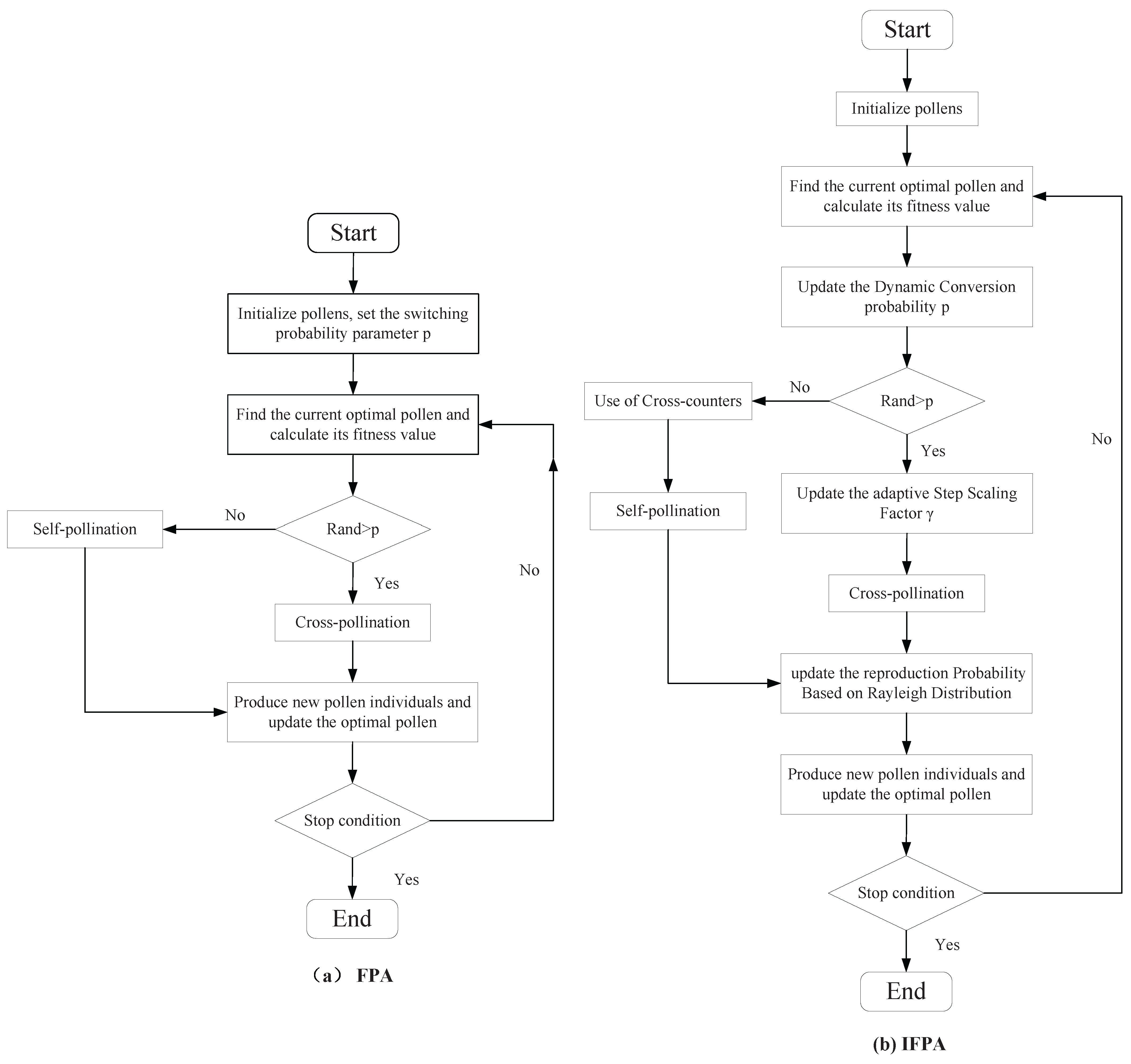
To clarify the process of the I-FPA, the flow chart is given in Figure 2, in which the left part is the diagram of the FPA and the right part shows the operations of the I-FPA. From Figure 2, it can be seen that four steps of the FPA are modified.

The switching probability p is dynamically adjusted according to the number of iterations. This adjusting can overcome local optimum and slow convergence. In the early stage, the dynamic switching probability p is small and the adaptive step size $\gamma$ is large due to the small number t of iterations. The algorithm tends to the global search which has high search efficiency. With the increasing of t, p becomes larger and $\gamma$ becomes smaller, and this makes the algorithm tend to the local search. This change lets the algorithm be able to find the optimal solution more quickly. The introduction of cross-counters $p_c$ improves the algorithm’s accuracy while simultaneously maintaining the diversity of the population. Hence, comparing with the FPA, the I-FPA has higher convergence rate and accuracy.

4. The Coverage Optimization Algorithm

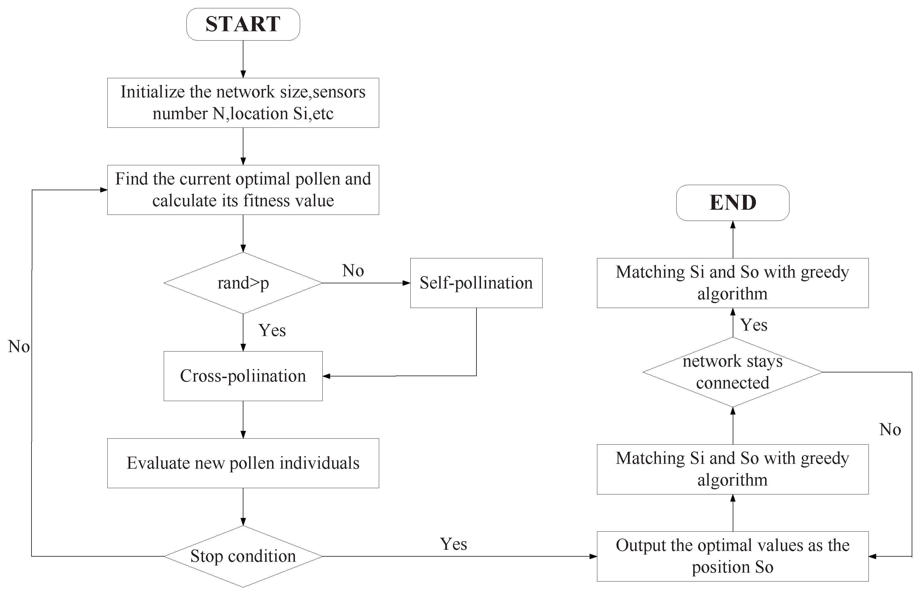
Based on the improved FPA, a coverage optimization is proposed, which is the coverage and connectivity based on the improved FPA (CCFPA). In the CCFPA, the I-FPA is used to find the optimal positions by considering the coverage quality and energy consumption. Then, a greedy node-matching algorithm is applied to complete node movement matching to achieve the purpose of minimum node movement distance. The flow chart of the proposed algorithm is shown in Figure 3, and the specific steps of searching the optimal positions and the matching process are given in Algorithm 1.

Algorithm 1: The improved FPA for WSN deployment

1: Input: $S_I$ : the set of initial locations sensor nodes. 2: Output: $S_o$: the set of optimal locations of sensor nodes. 3:   for t=1 to T(MaxGenerations) 4:      for i=1 to N(size Of population) 5:            $p=q-w·(1-t/T)$ 6:            if rand<p 7:                 Adaptive step scaling:$\gamma =\mu ·T·e^{-t/T}$ 8:                 Global Pollination:$X_i^{t+1}=X_i^t+\gamma L(X^{best}-X_i^t)$ 9:                 update the $X^{best}$ 10:           else 11:             Partial pollination:$X_i^{t+1}=X_i^t+\epsilon (X_j^t-X_k^t)$ 12:           Performing cross-operations 13:          Calculate the fitness of new flowers and renew in the population if the new flowers are better 14:          end if 15:    end for 16:  end for 17:  get Best flower $X^{best}$, as the set of the optimal locations of sensor nodes $S_o$. 18: Apply greedy node matching algorithm to match $S_I$ and $S_o$ for node movement 19: Determine whether the network is connected or not, and if not, select the next best set of deployment options until the connected set of options 20: Return: $S_o$: the set of the optimal locations of sensor nodes.

As shown in Algorithm 1, given the network parameters, they are mapped into parameters of the I-FPA and the fitness function is constructed by using the objective function. Then, the I-FPA is used to search for the best flower. When the stop condition is satisfied, the set of best flowers is output. The set of best flowers is the set of the optimal locations of sensor nodes.

In the coverage optimization of the WSN [31], position-finding and sensor movement are separately operated. The initial position set of N sensor nodes in the region is $S_I=\left\{s_1,s_2,...s_N\right\}$, and the final node position set after moving is $S_o=\left\{s_2^{\prime },s_2^{\prime },...,s_N^{\prime }\right\}$. The matching of $S_I$ with $S_o$ is achieved often by the greedy node-matching algorithm to move the sensor node to the target with the same serial number. To find the right position, the computation for N nodes moving toward N target locations is $N!$. When the number of sensor nodes is large, the algorithm is too computationally intensive. In addition, the average node movement distance is usually not the shortest. Therefore, to achieve the goal of minimum energy consumption for node movement, the greedy node-matching algorithm is proposed in this paper, and its pseudo-code is shown in Algorithm 2.

Algorithm 2: Greedy node-matching algorithm

1: Input: the initial position of sensor nodes $S_I$, the optimal position after moving $S_o$,the number of mobile nodes N. 2: Output: the node assignment diagram 3:   for i=1 to N do 4:         for j=1 to N do 5:            calculate for $d_{ij}=\left|S_i{S}_j\right|$,$S_i\in S_I,S_j\in S_o$, 6:              append to set D 7:         end for 8:   end for 9:   for k=1 to N do 10:        find the shortest distance $d_{ij}$ in D, complete a 11:          pair of node matches $S_i,S_j$. 12:        Matching nodes do not participate in the next 13:          round of matching. 14:   end for 15: Return: Draw the node assignment diagram

In the FPA algorithm, the time complexity is only related to the number of iterations T, the population size N, and the search dimension D. The time complexity of the FPA is $O(N·T·D)$. On this basis, the improved FPA adds some operations which bring more time complexity. The added operations are used to calculated the adaptive step scaling, the reproduction probability based on Rayleigh distribution, and the dynamically adjusted transition probability, which have the same size as the number of iterations. Hence, the time complexity of the I-FPA $O(N·T·D+3T)$. In the greedy node-matching algorithm, the distance between each sensor and each position should be calculated and sorted; thus, the number of operations is $N^2$. In addition, the connectivity judgment increases the number of operations by $O(N·N)$. Therefore, the time complexity of the proposed algorithm is $O(N·T·D+3T+2N·N)$.

5. Numerical Results

The simulation validation in this section contains two types of experiments. To prove the effectiveness of the I-FPA, we first compare the convergence performance of the improved FPA with four other well-known metaheuristics, including the FPA on four standard mathematical functions. Then, the second experiment applies the proposed algorithm to WSN for coverage optimization to verify the performance of the CCFPA.

5.1. Function Testing and Analysis

Like other metaheuristics publications, the I-FPA is evaluated by using a set of standard functions. Four baseline functions will be selected, and they are all minimization problems with optimal solutions of 0. They were chosen because each function has a unique set of qualities that make it easier to assess metaheuristic algorithms. The four specific test functions are shown in

Table 1. Standard test functions.

Function	Dimension	Variable Range	Theoretical
$F_1={\sum }_{i=1}^n{x}_i^2$	30	$[-100,100]$	0
$F_2={\sum }_{i=1}^{D-1}[100{(x_{i+1}-x_i^2)}^2+{(x_i-1)}^2]$	30	$[-30,30]$	0
$F_3=\frac{1}{4000}{\sum }_{i=1}^n{x}_i^2-{\prod }_{i=1}^{n}cos\left(\frac{x_i}{\sqrt{2}}\right)+1$	30	$[-600,600]$	0
$F_4=-20exp(-0.2\sqrt{\frac{1}{D}{\sum }_{i=1}^D{x}_i^2})-exp(\frac{1}{D}{\sum }_{i=1}^{D}cos2\pi x_i)+20+e$	30	$[-32,32]$	0

. It is evident that $F1$ is unimodal and separable, while $F2$ is non-separable. $F3$ and $F4$ functions have multimodal and non-separable characteristics.

By using these four test functions, our proposed I-FPA compares with other four algorithms: FPA, AIFS [32], IGWO [33], and IPSO [34]. The improved FPA is set to the same population size and number of iterations with the comparison algorithms, and 20 independent runs were performed for each of the four groups of test functions in Table 1. The best, average, and worst values of each algorithm are collected and compared. The comparison results are given in

Table 2. Test results.

Function	Evaluation Metrics	IGWO	FPA	AIFS	IPSO	I-FPA
$F_1$	Best	0.0052	0.2609	0.1602	0.5040	1.054 $\times {10}^{-3}$
	Average	0.1851	0.3602	8.089 $\times {10}^{-3}$	0.6565	1.809 $\times {10}^{-3}$
	Worst	0.3563	0.4602	1.600 $\times {10}^{-3}$	0.8090	1.419 $\times {10}^{-3}$
$F_2$	Best	0.0334	0.8819	0.7574	0.6139	2.528 $\times {10}^{-2}$
	Average	0.6852	2.026	0.9177	1.3318	7.573 $\times {10}^{-2}$
	Worst	1.2165	4.1239	1.0780	2.0496	4.674 $\times {10}^{-2}$
$F_3$	Best	0.5926	0.6144	0.7584	0.5334	7.038 $\times {10}^{-3}$
	Average	1.2038	0.3280	1.8069	3.1942	2.609 $\times {10}^{-3}$
	Worst	3.0938	1.0316	2.8554	5.8550	1.337 $\times {10}^{-2}$
$F_4$	Best	5.043 $\times {10}^{-3}$	2.2700	2.8260 $\times {10}^{-2}$	1.8050	4.44 $\times {10}^{-3}$
	Average	4.764 $\times {10}^{-2}$	3.4450	0.1311	2.3105	1.572 $\times {10}^{-2}$
	Worst	9.025 $\times {10}^{-2}$	4.6200	0.2340	2.8160	2.7 $\times {10}^{-2}$

, where our results are highlighted in bold.

From the comparison results in Table 2, it can be obtained that the proposed I-FPA is the best among five algorithms in terms of the search accuracy for both single-peak and multi-peak functions. This indicates that the improved algorithm can effectively go beyond the local optimum and search in the direction of the global optimum. Moreover, the optimal values obtained by the I-FPA are most closed to the optimum solution 0, whether it is the best, average, or the worst. The gap of the I-FPA with the optimum solution 0 is two magnitudes less than that of the other four algorithms on some metrics of a certain function.

In addition to the comparison of the accuracy of the results, Figure 4 presents the convergence plots of five algorithms running the four test functions. From the results in Figure 4, the convergence rate of the FPA is far faster than other four algorithms.

From the above figure, it can be seen that the improved FPA algorithm significantly improves the search accuracy and convergence performance of these four functions as the number of iterations increases. In the later iterations of the algorithm in particular, the improved FPA still has the effect of continuous optimization. The results show that the proposed algorithm has good global search ability, can effectively avoid local extremes, and converges faster.

5.2. WSN Coverage Optimization Simulation

The improved PFA algorithm is then applied to WSN coverage optimization. The simulation environment is set as a flat area with $100\times 100{\mathrm{m}}^2$. A total of 80 mobile nodes are randomly deployed with sensing radius $R_s=8.8375\mathrm{m}$, and the communication radius $Rc=17.675\mathrm{m}$. The population size is 50, the maximum number of iterations is 20, and the initial energy $E_0=0.5\mathrm{J}$. Figure 3 depicts the effect of the improved FPA on the network coverage optimization, where the circle indicates the sensing range of sensor nodes, and the signal * indicates the monitoring target point. The blue points represent the sensor nodes and the red points are the monitoring target points. The green circles indicate the sensing range of sensor nodes.

Figure 5a shows the covera situation of random deployment of sensor nodes. The coverage rate of the network in Figure 5a is $88.9\%$. It can be seen that sensor nodes are not evenly distributed, and many target points are not covered. At the same time, the distance from the sensor node to its neighbour sensor nodes is greater than $Rs$, and the network is disconnection. After using the proposed CCFPA, the node coverage state is shown in Figure 5b. All target points are covered, and the coverage rate is $100\%$. Each sensor node has at least one sensor node in its transmission range, which indicates that the network is connected. Thus, the proposed algorithm can effectively solve the coverage hole problem and disconnectivity.

Figure 6 depicts the coverage comparison of the WSN by using the FPA algorithm, IGWO algorithm, and the improved algorithm, respectively, for monitoring target points with different numbers of deployed sensor nodes. It can be seen from the figure that when the number of sensor nodes is 50, coverage optimization schemes based on the IGWO and the improved FPA can cover all monitoring target points $100\%$, whereas the FPA algorithm needs 65 sensor nodes to achieve complete coverage. The algorithm using the I-FPA only needs 20 iterations to achieve full coverage of monitoring target points, whereas the algorithm adopting the IGWO algorithm needs 50 iterations to achieve full coverage. Thus, the CCFPA has the best coverage optimization capability for the WSN with the random deployment.

High coverage and low energy consumption are two main objectives considered in the coverage optimization of wireless sensor networks. The energy consumed by the sensor movement is shown in Figure 7. The consumed energy increases with the increasing number of sensor nodes. This is because the selected sensor nodes also increase when the deployed sensor nodes increase. The energy consumption of the network utilizing the proposed CCFPA is smaller than that of other two algorithm. First, as proven in Section 5.1, the I-FPA used by the CCFPA has higher accuracy than the FPA and the IWGO, the position set found by the CCFPA is closer to the optimal position. Secondly, the greedy node-matching algorithm is used by the CCFPA to match the sensor nodes and the optimal position, and the shortest movement distance can be achieved. Thus, sensor nodes consume the least energy when the coverage is guaranteed.

6. Conclusions

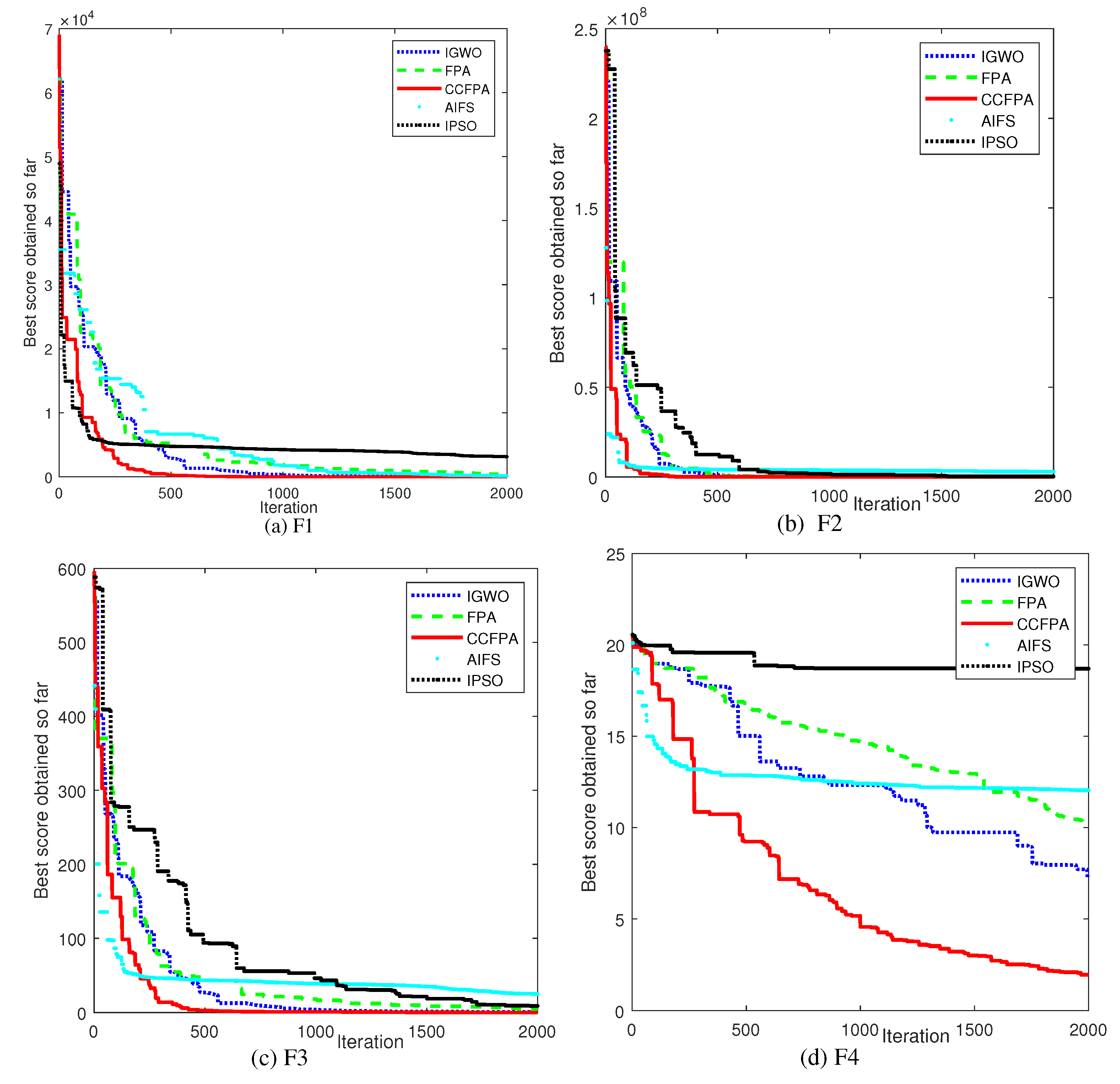
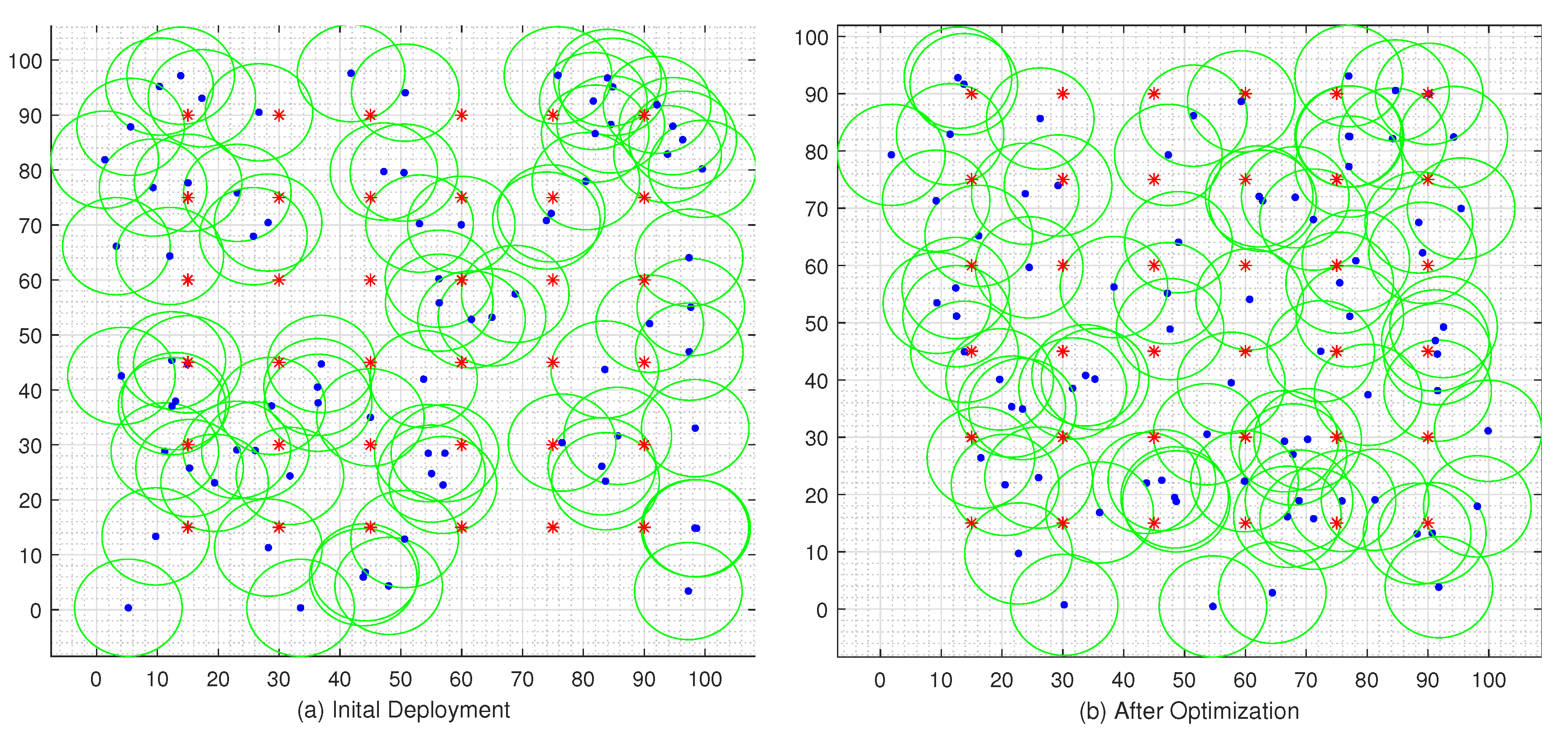
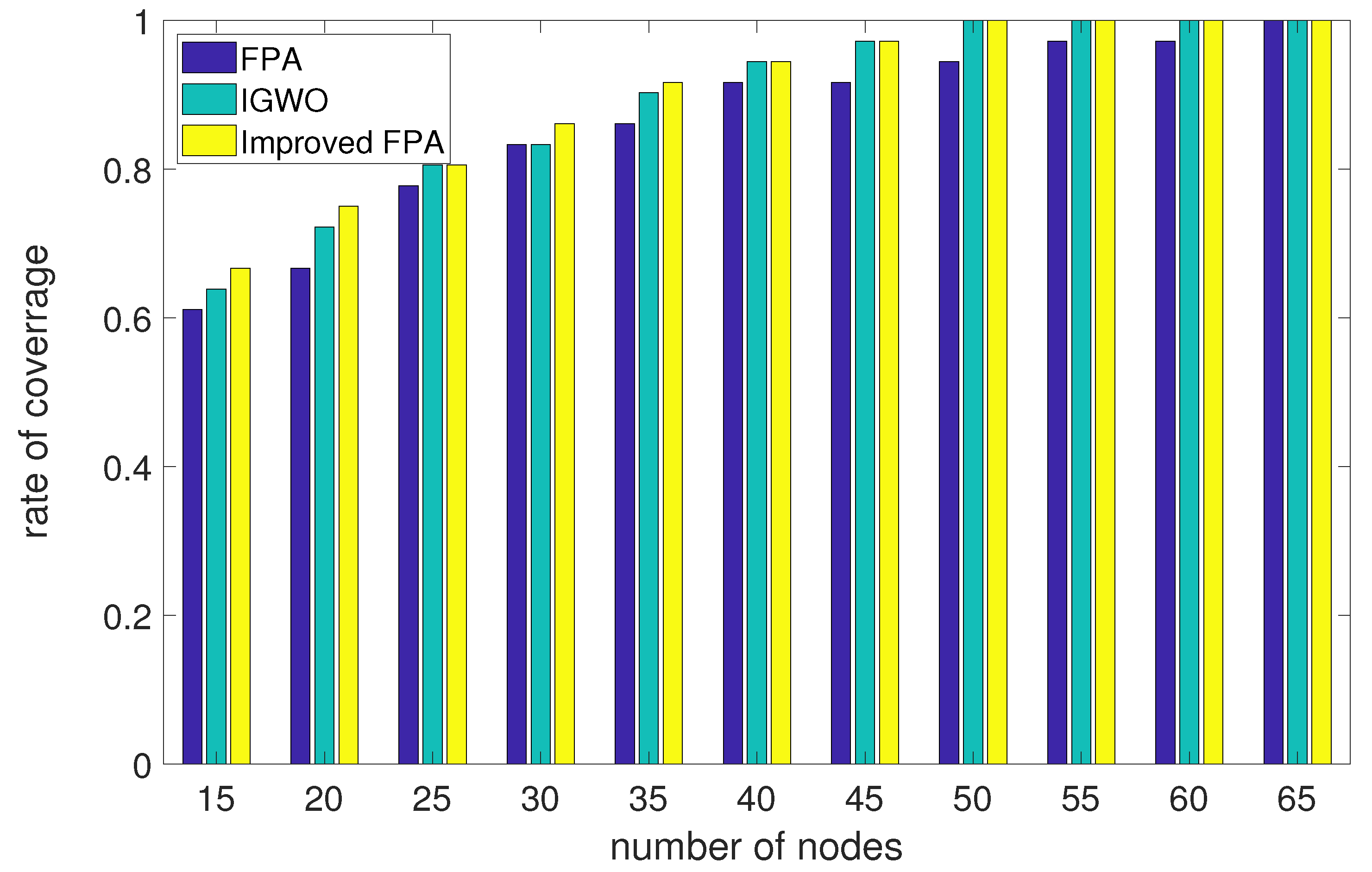
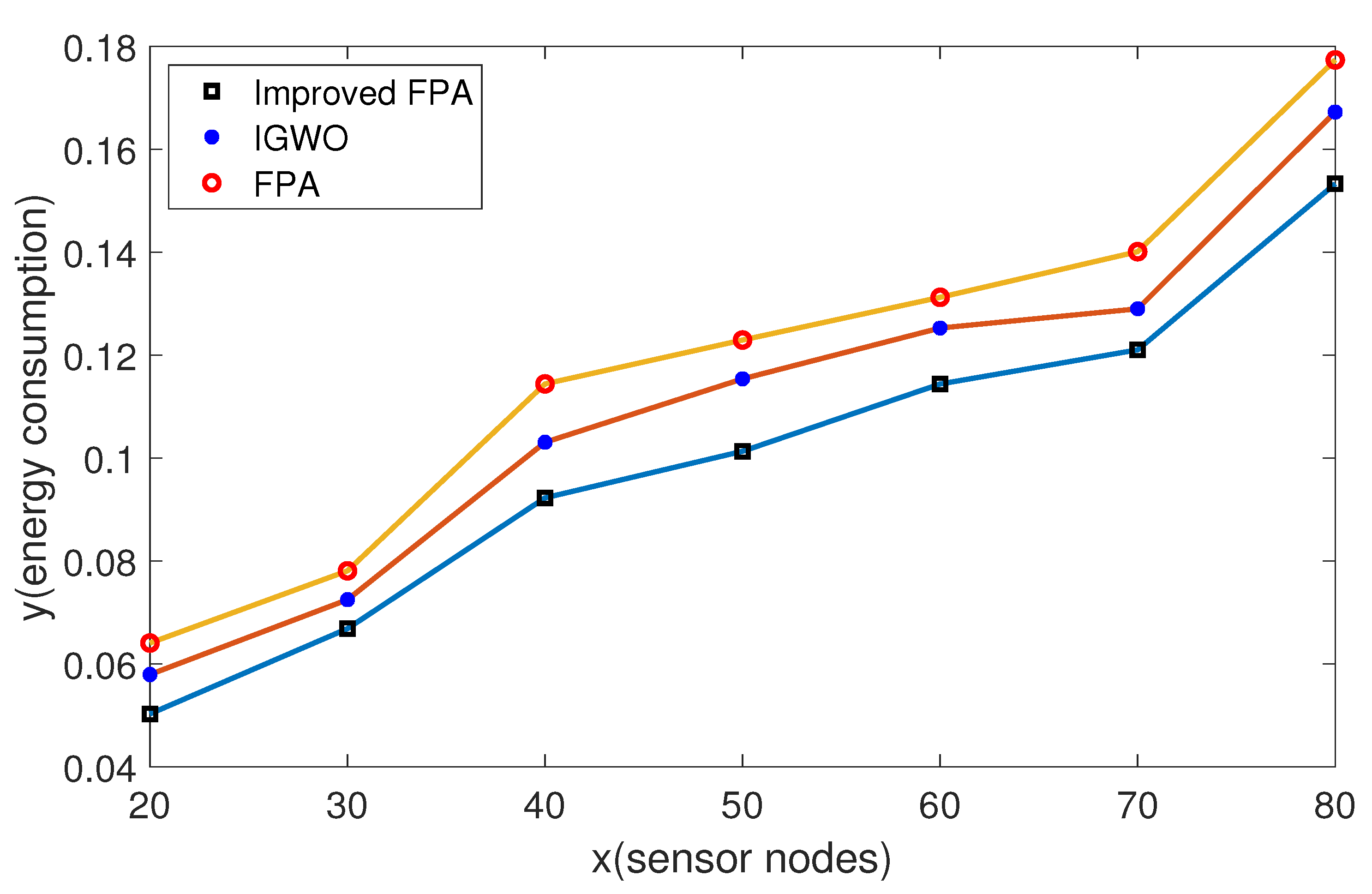
To solve the problem of node coverage optimization in wireless sensor networks, a new algorithm is proposed to optimize the network coverage. First, to address the shortcomings of slow convergence and insufficient accuracy of the FPA, an improved flower pollination algorithm is proposed. The I-FPA improves its global pollination capability and enables itself to explore more regions in the search space to avoid falling into local extrema. Besides, the improvement of local pollination enhances the ability to search widely for the optimal solution; thus, the convergence of the near-optimal solution speeds up in the right direction. In addition, the introduction of the crossover operator in local pollination maintains the diversity of the population and improves the convergence accuracy of the algorithm. Then, based on the I-FPA, a coverage and connectivity optimization algorithm (CCFPA) which considers the coverage quality, mobile energy consumption, and the network connectivity is proposed. The CCFPA utilizes the I-FPA to find optimal positions where sensor nodes would move and the greedy node-matching algorithm to determine which sensor node move to a certain position. By using four typical standard functions, the comparison of the test results demonstrates that the I-FPA has higher search efficiency and accuracy than the standard FPA, IGWO, AIFS, and IPSO. The simulation results verify that our proposed CCFPA can use fewer sensor nodes and less movement energy to guarantee 100% coverage and connectivity.

In this work, the coverage optimization of the WSN with random deployment is realized by moving some sensor nodes. Hence, the selection of sensor nodes and positions is the key point of the problem. We assume that all sensor nodes can move; however, some sensor nodes cannot move in practical applications. Thus, combining dynamic sensors and static sensors to optimize the coverage of the WSN is an interesting topic. Furthermore, in the future Internet of things, not only the sensor node can move, and both the sink and relays are mobile. The coverage optimization of the WSN becomes more complicated.