Article

Development of a Methodology for the Conservation of Northern-Region Plant Resources under Climate Change

1
Department of Environmental Science and Ecological Engineering, Korea University, Seoul 02841, Korea
2
Division of Technical Supervision, Green Technology Center, Seoul 04554, Korea
3
Ojeong Resilience Institute, Korea University, Seoul 02841, Korea
4
Department of Land and Water Environment Research, Korea Environment Institute, Sejong 30147, Korea
5
Department of Life Sciences, College of Natural Science, Yeungnam University, Gyeongsan 38541, Korea
*
Author to whom correspondence should be addressed.
Forests 2022, 13(10), 1559; https://doi.org/10.3390/f13101559
Submission received: 11 August 2022 / Revised: 14 September 2022 / Accepted: 20 September 2022 / Published: 23 September 2022

Abstract

:
According to the guidelines of the Nagoya Protocol, species are now recognized as ‘resources’ and owned by each country, thereby emphasizing the significance of biological resources and the importance of the continuous efforts made to systematically manage them. Despite these efforts, climate change, which influences climatic factors such as temperature and precipitation, is expected to negatively impact the struggle for conservation of biological resources by affecting species’ habitats. We aimed to devise methodologies that could be utilized for the management of biological resources, especially valuable tree species, that are experiencing difficulties due to climate change. First, changes in habitat of the northern-region plant Needle fir (Abies holophylla) due to of climate change were estimated using the BIOMOD2 package in R under the RCP8.5 scenario. Second, the time period of management was estimated based on the change in habitat area over time. It is expected that 30% of the current habitat of A. holophylla will be lost by 2030 and 50% will be lost by 2042. Third, four management zones (maintenance, reduction, dispersal, and non-habitat areas) were derived by comparing habitats according to the period of management required. In this case, we compared the present and the time point at which 30% habitat loss (2030) is expected to occur. After that, the management steps that can be taken for each management zone were suggested. Our results show the impact of climate change, especially change in Bio1 (annual mean temperature) and Bio13 (precipitation of wettest month), on species distribution patterns and have potential applicability in biological resource management. We have specified the suitable point of time, area, and direction of management in this study, which will contribute to climate change management planning and policy-making. By doing so, we hope that when a management policy on biological resources is applied, by dividing the four management zones, policymakers will be able to apply a cost-efficient policy.

1. Introduction

Global warming, a representative example of climate change, is an increase in the average temperature of the sea and the Earth’s surface. From 1906 to 2005, the global average temperature rose by 0.74 ± 0.18 °C [1]. In South Korea, the average temperature increased from 1912 to 2017 by 1.4 °C, which is approximately twice the global average temperature change [2]. During the last glacial maximum (LGM), which occurred approximately 20,000 years ago, the temperature was lower than 5 °C [3]. The rate of climate change is gradually accelerating, and the global temperature is expected to rise by more than 2 °C for Representative Concentration Pathways (RCP) 4.5 and 4 °C for RCP8.5 by the end of the 21st century [4].
Climatic factors such as temperature and precipitation affect species habitats, and climate change influences organisms that are adapted to the natural environmental conditions. Plant species are more vulnerable to climate change than animal species because they lack mobility and resistance to temperature changes, and the risk to plant species in areas having high levels of plant diversity and endemism is significantly higher [5], which has forced these species to move northward toward higher elevations [6]. Therefore, conservation measures are urgently required to increase the external adaptation potential of endemic biota.
Most countries import the raw materials that are obtained from plant species, which are used in the cosmetic and pharmaceutical industries for making anti-aging, anti-cancer, or anti-inflammatory agents; for example, in South Korea, approximately 80% and 54.4% of the cosmetic and pharmaceutical sectors, respectively, import a significant portion of their biological source material [7]. Therefore, conservation of domestic species, which are important biological resources, is necessary.
To maintain biological resources for a long term, it is necessary to determine the direction and urgency of conservation by identifying the characteristics of each biological resource, investigating the current distribution area, and predicting the future distribution area (due to climate change). Nowadays, research is being conducted to understand the impact of climate change and devise conservation strategies targeting domestic medicinal plants and cultivated crops [8,9]. In South Korea, previous researchers have mainly focused on Korean Abelia (Abeliophyllum distichum) and Korean fir (Abies koreana), because very few of these plants are left in the wild and their distribution area is expected to decrease further owing to climate change [10,11]. Studies have also been conducted on species showing similar biological characteristics, such as evergreen broadleaf trees of the family Lauraceae and warm-temperate evergreen broadleaf trees [12,13]. The present study was conducted on Abies holophylla, a near threatened species according to the International Union for Conservation of Nature (IUCN) Red List [14], which considers the threat from factors such as logging and forest fires, not climate change.
One of the policies implemented to conserve biological resources is the species status assessment (SSA) framework under the United States Endangered Species Act (ESA), which predicts change in species distribution or population size by identifying the species’ ecological characteristics and integrating scenarios such as loss of connectivity and habitat due to disasters [15,16]. The second policy is the habitat conservation plan (HCP), which analyzes the environmental impact of infrastructural projects or geographical changes on the species and provides suggestions on the prevention and mitigation of the negative effects [16,17]. However, the HCP allows “incidental take permits” for threatened or endangered species; questions are being raised on its effectiveness in species protection [18]. Further, the disadvantages of these policies are that the SSA is not involved in policy-making and the HCP does not predict the large-scale impact of developmental projects because it only focuses on the target project site and its vicinity.
The existing reports and policies are focused on analyzing habitat change trends, major factors influencing climate change, and extinction of target species, not on the management of biological resources. Therefore, the purpose of this study was not only to identify habitat change trends under climate change, but also to devise a biological resource management plan. The pattern of habitat change over time was derived using the species distribution model (SDM) for plants growing in northern regions that are negatively affected by global warming. We attempted to formulate a biological resource management plan for species affected by climate change by defining an appropriate unit period (time period of management) and classifying management areas for biological resource conservation.

2. Materials and Methods
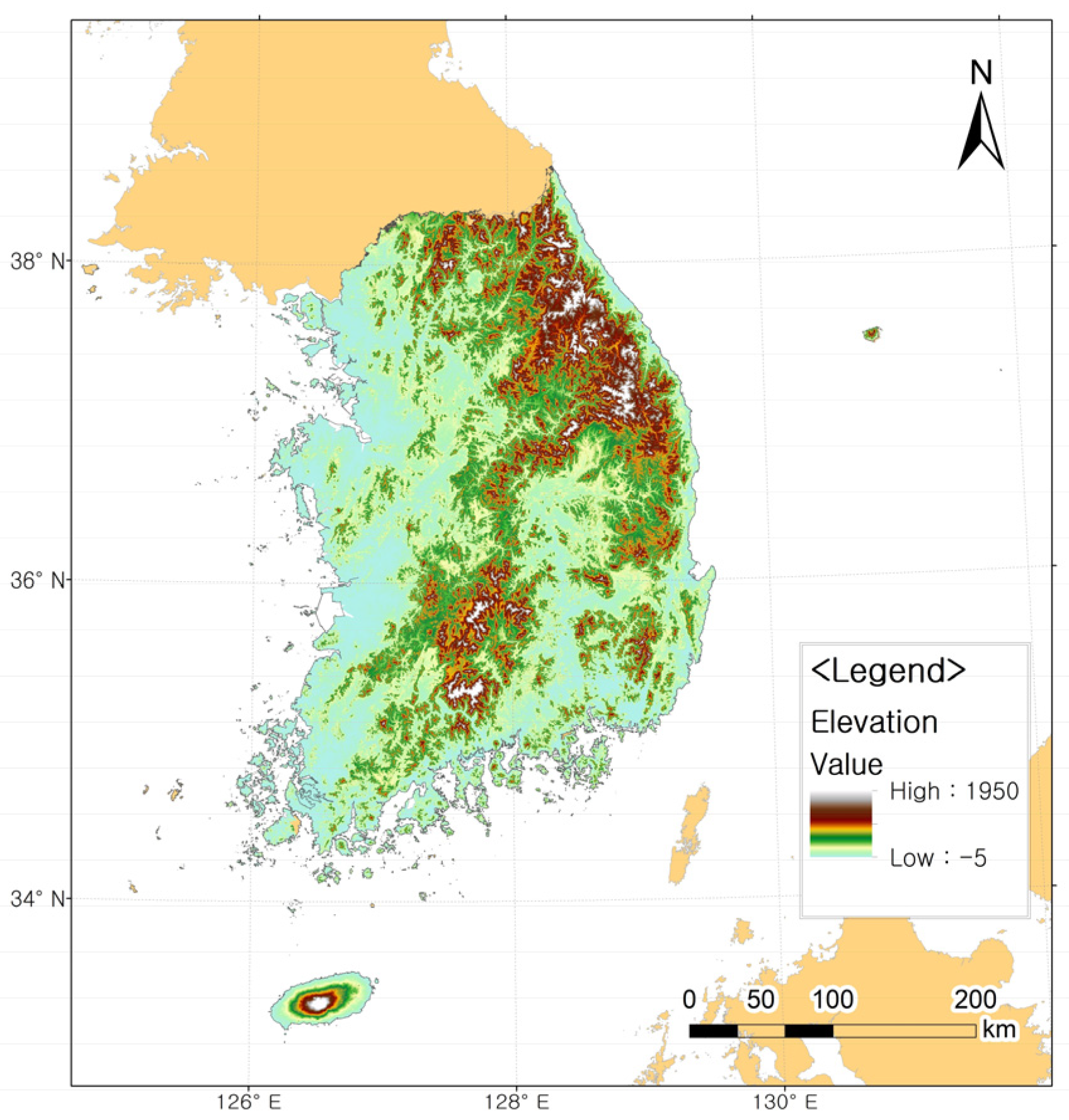
2.1. Study Area

The study site, South Korea, is a peninsula protruding from the eastern tip of the Eurasian continent with a total area of 100,210 km2, is surrounded by the sea on three sides, and borders North Korea at 33°–38° N and 125°–131° E (Figure 1). Located in the mid-latitude region of the northern hemisphere, it has a temperate climate of four seasons, with hot and humid summers due to the influence of the North Pacific air mass, cold dry winters because of the Siberian air mass, and relatively short spring and fall seasons. The average annual precipitation is 1292 mm, of which about 41% is concentrated in the summer months, especially in July and August [19]. The average annual temperature was 12.6 °C in the past (1912–1941) and is 14.0 °C at present (1988–2017), suggesting an average temperature increase of about 1.4 °C in this time period; the lowest and highest temperatures also rose by 1.1 °C and 1.9 °C, respectively, indicating an overall rise in temperature [2].

2.2. The Target Species

We selected 100 plant species that grow in the northern region from the list ‘300 Target Plants Adaptable to Climate Change in the Korean Peninsula’ [20]; among them, woody plant species with at least 100 coordinates were selected based on the third and fourth National Ecosystem Survey (NES) data (2006–2018) provided by the National Institute of Ecology. The NES, which was initiated in 1986, is a nationwide survey that includes endemic as well as alien and invasive species. It contains reliable data assembled using information gathered from GIS-DB, such as details about presence and habitat of the species, and is registered under the Global Biodiversity Information Facility (GBIF).
Finally, based on a review of previous studies, the species A. holophylla was selected because of its economic importance (Table 1). A. holophylla is the evergreen tree of the conifer family of Pinaceae. It has needle-shaped leaves and cylindrical fruits. With its flowers blooming in late April and fruits ripening in early October, this representative tolerant tree grows very slowly for the first seven or eight years but grows with an increasing growth rate afterwards, even well in the shade of other trees [21,22]. A. holophylla inhabit the same areas with various plants: conifers such as Korean pine (Pinus koraiensis), Sword fern (A. nephrolepis), and Olga Bay larch (Larix gmelinii (var. olgensis)), and broad-leaved trees such as Mongolian oak (Quercus mongolica), Manchurian ash (Fraxinus mandshurica), and Erman’s birch (Betula ermanii) [14].
A. holophylla has been designated “near threatened” by the IUCN, and the main threat is unrestricted logging. It is classified as “threatened” on applying criterion A2d of the IUCN Red List. It is distributed throughout northeastern China, southeastern Siberia, and South Korea, and generally inhabits mountainous areas (10–1200 m above sea level in high-latitude areas and 500–1500 m above sea level in low-latitude areas) with cold climatic conditions (characterized by heavy precipitation in summers and dry winters), which remain covered with snow for most of the year [14].
Most plant species are not able to adapt swiftly to the climate-driven changes in their habitat [23]. In particular, the genus Abies is under threat from climate change because the seed dispersal length is short (approximately 100 m), and the time it takes to reach the reproductive stage is long (approximately two years) [24,25].

2.3. Species Distribution Model (SDM)
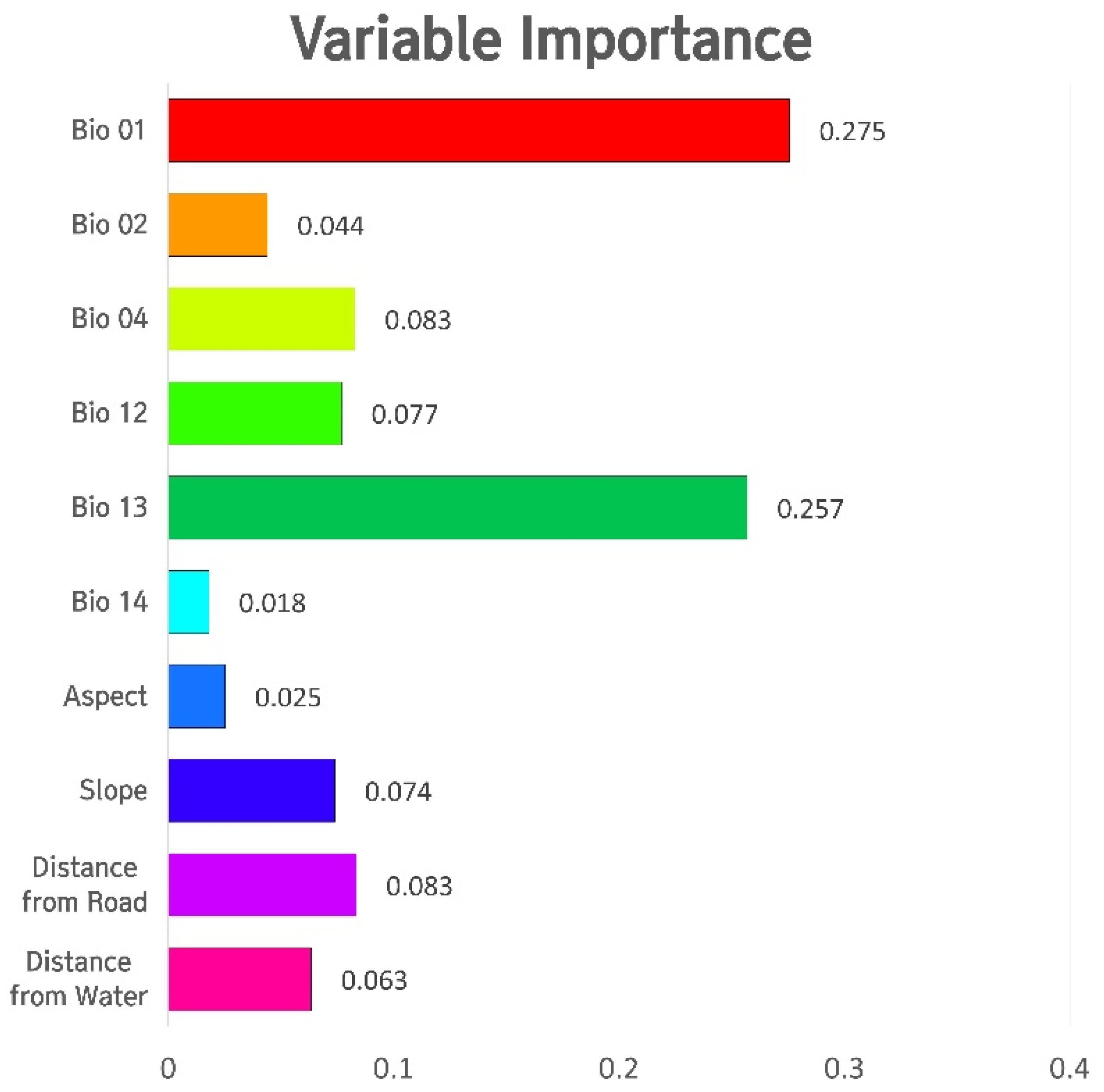
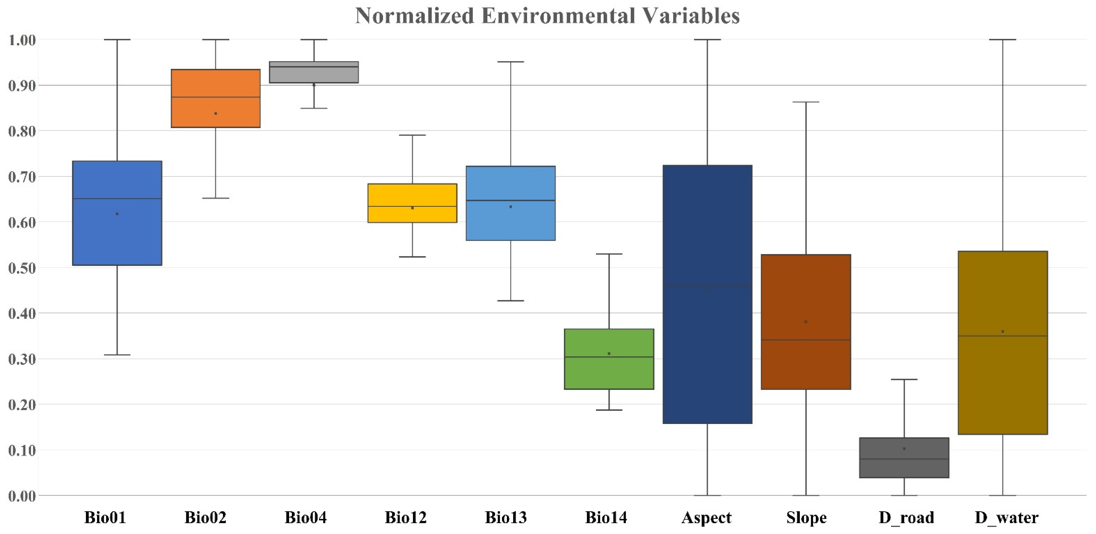
The BIOMOD2 package in R was designed for modeling species distribution using species presence/absence data. The package uses 10 modeling methods (generalized linear model [GLM], generalized additive model [GAM], generalized boosting model [GBM], multiple adaptive regression splines [MARS], flexible discriminant analysis [FDA], classification tree analysis [CTA], random forest [RF], artificial neural network [ANN], surface range envelop [SRE], and maximum entropy [MaxEnt]), and is capable of ensembling single models, as well as generating predictions on future climates through a future climate projection function. In this study, seven of the models (GLM, GBM, MARS, FDA, CTA, RF, and ANN) were used to estimate species distribution, and ensembles were developed using models with a true skill statistic (TSS) value greater than 0.6 [26].
GLM is a linear regression model [27,28], while GBM is a machine learning technique that learns in the direction that approaches the actual value using the mean as an initial estimate [27,29]. MARS is a linear regression technique that can model nonlinearity [28]. FDA is also called linear discriminant analysis, as it is a combination of linear regression models and uses optimal scoring to transform response variables so that linear separation of the data can be performed [28]. CTA is a prediction model that utilizes decision trees to link observations and targets for an item [27,28]. RF is a machine learning-based ensemble technique that uses decision trees [27,30], and ANN is a machine learning technique that derives results based on the strength of connection between variables [31].

2.4. Variables

The environmental variables used to predict the species distribution were selected considering the ecological characteristics mentioned in the previous studies on A. holophylla [14,32], and were classified into climatic and topographical factors. All environmental variables were unified as grids in units of 30 arcseconds (approximately 1 km) corresponding to the location of the climate data source.
Raw data on measured values of environmental variables corresponding to climatic factors were provided by the Korea Meteorological Administration. The current climate represents the years 2000–2019, and the future climate is the raster dataset, which was statistically downscaled using the modified Korean parameter-elevation regressions on the independent slopes model (MK-PRISM) technique coupled with the HadGEM3-RA model. HadGEM3-RA is a dynamic regional climate model downscaled from HadGEM2-AO, developed by the Hadley Center in the UK, and is used as a national standard scenario by the Korea Meteorological Administration [33].
There is no doubt that Shared Socio-economic Pathways (SSPs) is the most up-to-date scenario, but there has been no study of which SSPs correspond to the current state. However, in RCPs, as the current and near-future climatic conditions are similar to the RCP8.5 scenario (based on the 5th report of Intergovernmental Panel on Climate Change [IPCC]), this scenario was selected [34]. The values of climatic variables fluctuate annually, so the moving average method, which represents a single year, is used to average figures over a certain period of time [26,35,36]. Here, a 25-year moving average was estimated by calculating the average of values recorded at a single point in time, and at 12 years before and after that point.
Variables corresponding to climatic factors were generated using the Biovars function in R. BioClim consists of 19 variables derived from measurement of precipitation, lowest temperature, and highest temperature; thus, some variables (showing similar tendencies) are multicollinear. We attempted to avoid multicollinearity by using principal component analysis (PCA) analysis to represent the total climatic factor. Six bioclimatic variables were examined in this study: Bio01, Bio02, Bio04, Bio12, Bio13, and Bio14 (Table 2).
The topographic factors comprised four variables: aspect, slope, distance from roads, and distance from water. Aspect and slope were calculated using elevation data (WorldClim 2.1) provided by WorldClim (https://www.worldclim.org/, 16 December 2021). The distance from roads was calculated using data on the national standard node link provided by the National Transport Information Center of the Ministry of Land, Infrastructure, and Transport (MOLIT, Sejong, Korea), and the distance from water was calculated using the river map provided by the Water Resources Management Information System (WAMIS (http://www.wamis.go.kr/, 26 February 2022)).

2.5. Evaluation Method

TSS was used for the evaluation of data. Our results indicated that the area under curve (AUC) of the receiver operating characteristic (ROC) curve violated the AUC theory when pseudoabsence data was used in place of true-absence data, and single measurement methods such as calculation of Kappa value, taking omission and commission errors into consideration, exhibited the same problem [37]. Due to the above-mentioned problems in the estimation of AUC and Kappa values, TSS is commonly used to verify the predictions of species distribution models [38,39,40]. Overall, TSS, AUC, and Kappa were used as auxiliaries to confirm that the results were explanatory.

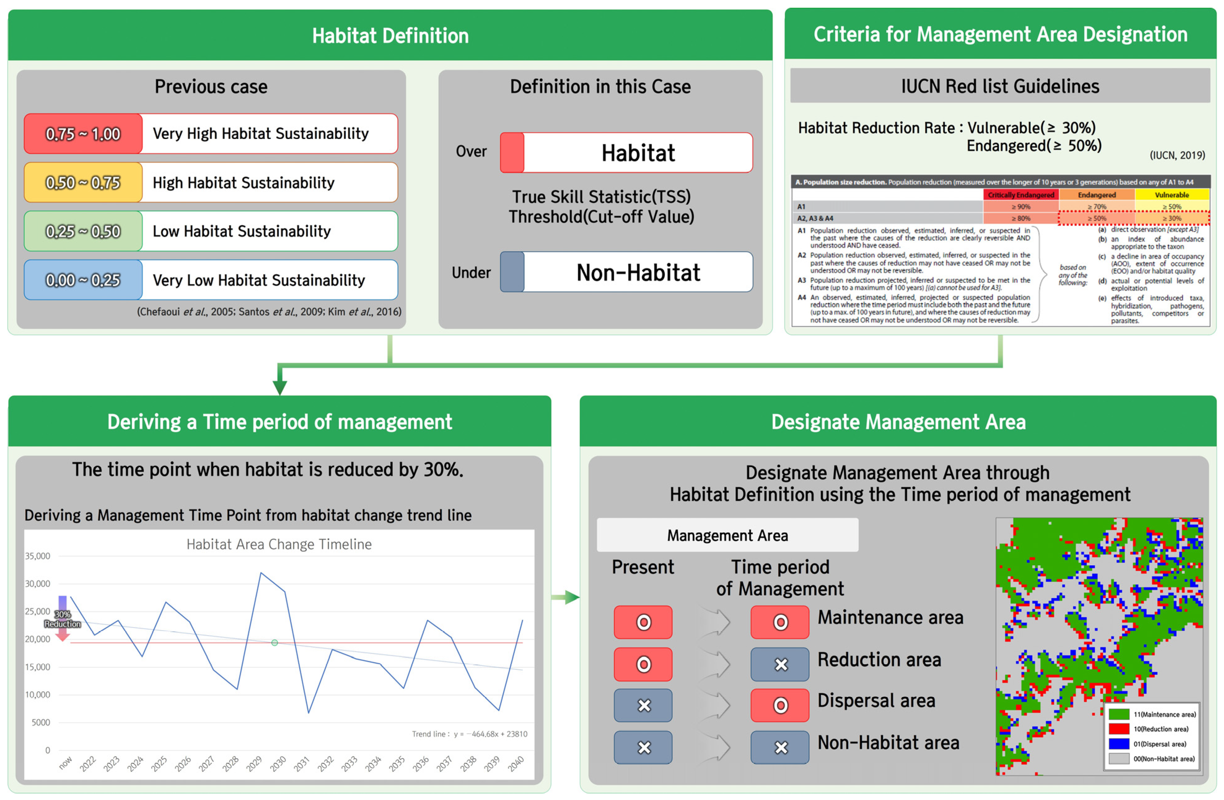
2.6. Time Period of Management and Management Area

To determine the time period for biological resource management, first, the potential habitat was defined, and second, the criteria to define the time period were set. Habitat was defined based on the probability distribution map, which was obtained from a previously performed BIOMOD2. The probability distribution map shows the probability of distribution of the species in each cell, and habitat is defined by identifying a threshold that is derived by modeling or dividing a particular interval. Out of all the accuracy verification methods mentioned above, we decided to use TSS, in which the accuracy was limited to the threshold; therefore, we used the threshold value of TSS derived through modeling.
The five evaluation criteria (A to E) of the IUCN Red List were used to define the time period of management. The criterion A is based on population reduction and is subdivided into four categories, from A1 to A4 [41]. In this study, we wanted to predict the future based on the current distribution, hence, it fulfilled the A3 criterion. To fall under one of the categories of threat in criterion A, certain thresholds representing population reduction must be met. In the rest of the steps (A2, A3, and A4), except for A1, the species is classified as critically endangered (CR) if it loses more than 80% of its population, endangered (EN) if the loss is more than 50%, and vulnerable (V) if the loss is more than 30%. We could not apply the IUCN standard directly because our study was geographically limited to South Korea. Therefore, we modified the IUCN category targeting the world to be more suitable for South Korea. In this process, the decrease in population, which was the criteria of IUCN, was replaced by the decrease in habitat area. Even though we replaced the variable, we also thought the quantitative criteria defined by the IUCN as a global standard could be applied to South Korea. The point where the habitat loss rate reached 30% or more, based on IUCN category vulnerability (Vulnerable [V]), was considered as the time period of biological resource management.
As the habitat of a species changes along with change in the climate, it is necessary to establish a biological resource management zone to manage biological resources. Biological resource management areas are classified into “maintenance areas” where habitats are maintained now and will be maintained in the future, “reduction areas” where habitats exist now but disappear in the future, “dispersal areas” where an area that is not currently a habitat will become a habitat in the future, and “non-habitat areas” that are not habitats in the present or the future (Figure 2).

3. Results and Discussion

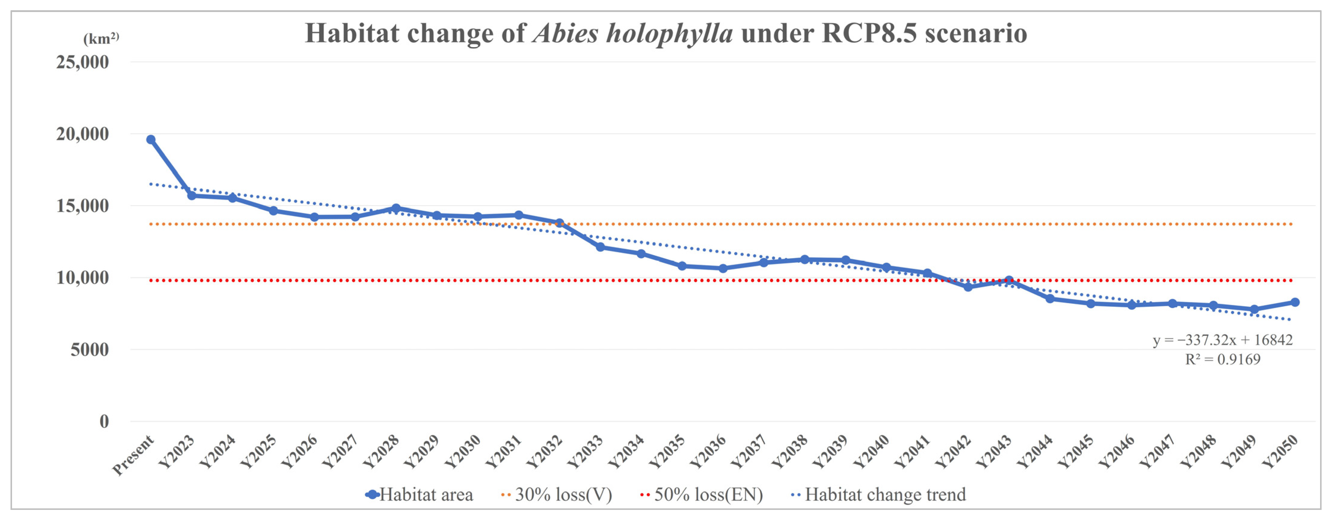
3.1. Analyzing Habitat Changes under Climate Change

The TSS value of the current distribution model of A. holophylla, calculated using BIOMOD2, was 0.703, indicating high accuracy of the presence and absence models. The Kappa value was 0.534, indicating that the classification is unlikely to be coincidental. The AUC value of the ROC (0.915) showed that the model was well-predicted and statistically reliable (Table 3). The cutoff value was 500 or more in all cases, confirming that the model predicts a high value of habitat suitability, despite using the existing method for classification of distribution probabilities that divides them into different sections. Overall, AUC and Kappa values validated the research methodology, and accuracy of the results was verified using the threshold value of TSS.
Variable importance differed for each model used in the ensemble (Table 4). Since the final result was an ensemble calculated using the simple average method based on the results of each model, the variable importance was also represented by a simple average. These values are depicted using a bar graph (Figure 3).
As a result of the modeling, it was found that Bio01 (annual mean temperature) and Bio13 (precipitation of the wettest month) had a significant influence on the distribution of A. holophylla. In particular, Bio01 was observed to show the highest influence by most of the single models except CTA and ANN; according to CTA, it showed the second highest influence. These results corresponded to the results obtained in previous studies showing that A. holophylla generally lives in areas having cold climates and heavy precipitation in summers [14]. The distance from the road variable showed the third highest influence, which validates the findings of previous studies that pollution caused by sulfur dioxide causes serious damage not only to fir trees but also to seedlings [42,43].
Based on the distribution of A. holophylla, the value of each variable corresponding to the current state was derived and compared with the general environmental characteristics of the species coordinates and South Korea (Table 5). There could be errors in comparing only the average value, so we attempted to analyze with the boxplot, which is made from normalized data (Figure 4).
The habitat of A. holophylla showed lower temperatures on average, and the average annual precipitation was relatively high. In case of aspect, the figures in the table showed a tendency to prefer the southeast, but when compared with the boxplot, the distribution of the data was relatively homogeneous, indicating that aspect had little effect. The distance from the road variable was found to be relatively distant compared to the South Korea average, which is thought to be because A. holophylla is affected by air pollution, as mentioned above.

3.2. Determining Time Period of Management

Fir trees are northern-region plants and their habitat is expected to slowly decline under RCP8.5. The current habitat area estimated using BIOMOD is 19,540 km2, accounting for approximately 20% of the total land area in South Korea. The models predicting habitat changes by 2050 showed that there would be a continuous decline from the current conditions.
The management period was determined by considering the trends of habitat change rather than by examining the habitattable area at a specific point in time. In the case of A. holophylla, it is predicted that more than 30% of the habitat will be lost by 2030 (about 8.2 years later), and more than 50% by 2042 (about 19.9 years later; Figure 5). Thus, it is necessary to establish a conservation plan with short-term goals for 2030 and mid- to long-term goals for 2042.

3.3. Management Area Classification

The management period provides a target time-point for the process of species conservation, and the classification of the management area is necessary for determining where and how to manage the biological resources. In order for policies on biological resource management to be effectively implemented, management areas should be classified while appropriate management measures should be applied for each management area. If a uniform method is applied to all areas, cost-effectiveness could decrease.
We have suggested four management areas: maintenance area, reduction area, dispersal area, and non-habitat area. The maintenance area is an area where habitats are maintained from the present to the future. The reduction area refers to an area where it is now a habitat, but not in the future. The dispersal area is now a non-habitat but is expected be habitat area in the future. The non-habitat area is an area where A. holophylla cannot inhabit from now to the future.
The species distribution model predicted that due to climate change, the current habitat area is expected to decrease by more than 30% by 2030 (approximately 8.2 years later). In the management area classification, the habitat at the current time and the habitat at the management period (Y2030) were compared. As for the classification of habitats, the probability map derived as a modeling result was converted to a binary map, which divided into habitat/non-habitat based on the threshold of the TSS. After that, four management areas were derived by overlapping the current and future binary maps.
Comparison of the current habitat (Y2022) with the habitat in the time period of management (Y2030) revealed that the maintenance area was 13,340 km2 (14.01% of the current habitat), the reduction area was 6272 km2 (6.59%), and the dispersal area was 901 km2 (0.95%). More than 50% decrease by 2042, that is, about 19.9 years later (Y2042), was predicted, where the maintenance area was 10,333 km2 (10.85%), the reduction area was 9279 km2 (9.74%), and the dispersal area was 385 km2 (0.40%) (Table 6).

3.4. Formulation of Plans for the Management Area

The four management areas were maintenance, reduction, dispersal, and non-habitat areas. The findings of the previous studies and our study showed that according to the distance from the road variable, sulfur dioxide contained in the smoke emitted from cars might affect the distribution of A. holophylla. Therefore, an environment similar to its habitat must be created by suppressing road development projects and regulating the access of vehicles in the management areas, except for non-habitat areas.
The management plans for each management area are as follows:
In the case of the maintenance area, the following two management directions can be suggested for maintaining the habitat from now to the time period of management. The first involves a non-intensive management method because in this case, the habitat is maintained without any special management required. Second, because the area is a high-quality habitat that lasts for a long time, it is conserved as a source of species diffusion. Assuming one maintenance area patch as an island, based on the island biogeography theory, it is possible to increase diversity and stability within the patch and conserve it [44], or to designate it as a protected area to insulate it from habitat disturbance [45].
In the reduction area, the current habitat becomes a non-habitat area in the time period of management. Considering that the factors having a significant influence on the distribution of A. holophylla are average annual temperature and precipitation in the wettest month, it is believed that the area has changed to a non-residential area due to climatic factors. Because it is impossible to create an environment similar to the species’ habitat by controlling climatic factors, considering realistic aspects, the individuals should be shifted to maintenance or dispersal areas [46], or their genetic resources should be collected for breeding purposes (e.g., seeds and seedlings).
The dispersal area is a non-habitat currently, but in the time period of management, it changes into a habitat. The habitat of a species is affected not only by climate, but also by soil and atmospheric conditions. For A. holophylla, more than 90% of the seeds are known to be dispersed within a radius of 50 m [47], and if the density of the tree-crown is not high, natural dispersal is known to occur well [48]. We can expect natural dispersal in the dispersal area, but we must consider ways to help the dispersal of A. holophylla because the spread distance of seeds does not keep up with the pace of climate change. In the case of soil, the depth less than 30 cm to bedrock and the composition containing gravel were known to be an obstacle to root growth, negatively affecting vertical growth, although it is known that poor soil environment negatively affects the proliferation of side roots and tiny roots even when sufficient depth is given [49]. Therefore, selecting an excellent area could be a important process to conservation. After that, an environment suitable for the habitat should be created through the actions such as identifying and removing the habitats of invasive and foreign species that hinder the growth of A. holophylla. In addition, ex-situ conservation can be achieved by planting seedlings in this area.
Non-habitat areas are areas where there is a very low probability that the species is inhabiting at present, and where it will not be found in the future as well, so it is unnecessary to devise a separate conservation plan for these areas.
Various factors are considered from a human point of view when establishing policies. We noted the need for species conservation in the area of responding to climate change and the importance of economical species due to the Nagoya protocol effect. In other words, the above four management areas are not only applicable to economically importance species such as A. holophylla, but are also applicable methods that can be used to conserve other species, from rare species to common species. However, there is a need to set a management method for each management area according to the characteristics of the target species.

4. Conclusions

A. holophylla, called the needle fir, grows in the northern regions of South Korea. Although it has a limited habitat in northeast Asia, the species is “near threatened.” The species A. koreana and A. spanish belonging to the same genus, are also designated as “near threatened” species and show regional distribution. In this study, our aim was to suggest a time period of management for the protection and conservation of northern-region plants and to propose some methods of management. The management method used for the conservation of one species, A. holophylla, can be extrapolated for management of the sympatric species of this plant.
Evaluation of management methods that have a reliable and consistent threshold as well as international relevance is difficult. It is difficult to apply the thresholds (e.g., cutoff) that were used in this study to other regions or compare them with other research methods, because the thresholds may vary from region to region. However, the target species is also distributed in northeastern China and southeastern Russia, which are geographically close to South Korea; therefore, it is expected that the threshold value can also be applied there. The connectivity between these countries will be considered in the follow-up studies for the preservation of this species.
Fir trees are expected to lose more than 30% of their total habitat by 2030 and approximately 50% of their total habitat by 2042, owing to a continuous decrease in habitat in South Korea (under RCP8.5). Therefore, the long-term preservation of their habitat is necessary. By comparing current and future habitats, management areas were identified and appropriate conservation plans for each management area were proposed. However, considering the limited budget and real-life situation, a comprehensive management plan that includes the sympatric species would be a more effective strategy than the strategy that targets a single species.
The limitation of this study was that we considered only the climate-change factor. In future, threat factors such as natural disasters, logging, or additional factors that reduce population size must be examined. Nevertheless, the results are meaningful and can be used for establishing a plan for effectively managing the endangered species that are influenced by climate change.

Author Contributions

Conceptualization, Y.Y., J.H. and S.J.; Formal analysis, Y.Y.; Investigation, Y.Y., Y.C., H.I.C., J.H., N.O.L., J.L., Y.K., M.J.K. and T.S.K.; Methodology, Y.Y., Y.C., H.I.C. and S.J.; Supervision, S.J.; Validation, Y.Y. and Y.C.; Visualization, Y.Y.; Writing—original draft, Y.Y.; Writing—review & editing, Y.Y., Y.C., Y.K. and S.J. All authors have read and agreed to the published version of the manuscript.

Funding

This research was funded by the Ministry of Science and ICT through Basic Science Research Projects of the National Research Foundation of Korea (NRF) (grant number 2021R1C1C2012406). This work was supported by Korea Environment Industry & Technology Institute (KEITI) through The Decision Support System Development Project for Environmental Impact Assessment, funded by Korea Ministry of Environment (MOE) (2021003360002).

Conflicts of Interest

The authors declare no conflict of interest.

References

  1. Trenberth, K.E.; Jones, P.D.; Ambenje, P.; Bojariu, R.; Easterling, D.; Tank, A.K.; Parker, D.; Rahimzadeh, F.; Renwick, J.A.; Rusticucci, M.; et al. Observations: Surface and Atmospheric Climate Change. In Climate Change 2007: The Physical Science Basis. Contribution of Working Group 1 to the 4th Assessment Report of the Intergovernmental Panel on Climate Change; Cambridge University Press: Cambridge, UK, 2007; pp. 235–336. [Google Scholar]
  2. National Institute of Meteorological Sciences. 100 Years of Climate Change on the Korean Peninsula; Korea Meteorological Administration, Ed.; National Institute of Meteorological Sciences: Jeju, Korea, 2018.
  3. Climap Project Members. Relative Abundance of Planktic Foraminifera in the 120 kyr Time Slice Reconstruction of Sediment Core GIK12392-1; PANGAEA: Bremerhaven, Germany, 1981. [Google Scholar]
  4. Korea Meteorological Administration (Ed.) Korean Cliamte Change Assessment Report 2020; Korea Meteorological Administration: Seoul, Korea, 2020.
  5. Klausmeyer, K.R.; Shaw, M.R. Climate Change, Habitat Loss, Protected Areas and the Climate Adaptation Potential of Species in Mediterranean Ecosystems Worldwide. PLoS ONE 2009, 4, e6392. [Google Scholar] [CrossRef]
  6. Davis, M.B.; Shaw, R.G. Range Shifts and Adaptive Responses to Quaternary Climate Change. Science 2001, 292, 673–679. [Google Scholar] [CrossRef] [PubMed]
  7. Lee, H.K.; Park, H.Y.; Kim, S.H. A Study on Planning for Joint Growth through Collaboration of Bio-Resources between Korea and Peru; Ministry of Science ICT, Ed.; Ministry of Science ICT: Sejong, Korea, 2017.
  8. van Treuren, R.; Hoekstra, R.; Wehrens, R.; van Hintum, T. Effects of climate change on the distribution of crop wild relatives in the Netherlands in relation to conservation status and ecotope variation. Glob. Ecol. Conserv. 2020, 23, e01054. [Google Scholar] [CrossRef]
  9. Cahyaningsih, R.; Phillips, J.; Brehm, J.M.; Gaisberger, H.; Maxted, N. Climate change impact on medicinal plants in Indonesia. Glob. Ecol. Conserv. 2021, 30, e01752. [Google Scholar] [CrossRef]
  10. Lee, S.-H.; Choi, J.-Y.; Lee, Y.-M. Projection of climate change effects on the potential distribution of Abeliophyllum distichum in Korea. Korean J. Agric. Sci. 2011, 38, 219–225. [Google Scholar]
  11. Koo, K.A.; Kim, J.; Kong, W.-S.; Jung, H.; Kim, G. Projecting the Potential Distribution of Abies koreana in Korea Under the Climate Change Based on RCP Scenarios. J. Korea Soc. Environ. Restor. Technol. 2016, 19, 19–30. [Google Scholar] [CrossRef]
  12. Yun, J.-H.; Kim, J.-H.; Oh, K.-H.; Lee, B.-Y. Distributional Change and Climate Condition of Warm-temperate Evergreen Broad-leaved Trees in Korea. Korean J. Environ. Ecol. 2011, 25, 47–56. [Google Scholar]
  13. Yu, S.-B.; Kim, B.-D.; Shin, H.-T.; Kim, S.-J. Habitat Climate Characteristics of Lauraceae Evergreen Broad-leaved Trees and Distribution Change according to Climate Change. Korean J. Environ. Ecol. 2020, 34, 503–514. [Google Scholar] [CrossRef]
  14. Katsuki, T.; Zhang, D.; Rushforth, K. Abies holophylla. In The IUCN Red List of Threatened Species 2013: E.T42287A2969916; IUCN: Gland, Switzerland, 2013. [Google Scholar]
  15. Smith, D.R.; Allan, N.L.; McGowan, C.P.; Szymanski, J.A.; Oetker, S.R.; Bell, H.M. Development of a Species Status Assessment Process for Decisions under the U.S. Endangered Species Act. J. Fish Wildl. Manag. 2018, 9, 302–320. [Google Scholar] [CrossRef]
  16. Wilkening, J.L.; Magness, D.R.; Harrington, A.; Johnson, K.; Covington, S.; Hoffman, J.R. Incorporating Climate Uncertainty into Conservation Planning for Wildlife Managers. Earth 2022, 3, 93–114. [Google Scholar] [CrossRef]
  17. Franklin, J.; Regan, H.M.; Hierl, L.A.; Deutschman, D.H.; Johnson, B.S.; Winchell, C.S. Planning, implementing, and monitoring multiple-species habitat conservation plans. Am. J. Bot. 2011, 98, 559–571. [Google Scholar] [CrossRef] [PubMed]
  18. Shilling, F. Do Habitat Conservation Plans Protect Endangered Species? Science 1997, 276, 1662–1663. [Google Scholar] [CrossRef]
  19. Heo, T.; Suh, E.; Kwon, W. Spatial analysis on the rainfall data by utilizing Variogram models. J. Korean Data Anal. Soc. 2004, 6, 473–491. [Google Scholar]
  20. Korea National Arboretum. 300 Target Plats Adaptable to Climate Change in the Korean Peninsula; Korea Forest Service, Ed.; Korea Forest Service: Daejeon, Korea, 2010.
  21. Kitapbaeva, A.A.; Kabataeva, Z.K.; Alipina, K.B.; Komekova, G.K.; Tuktassinova, A.A. The research of winter hardiness and seasonal development of some woody plants in East Kazakhstan. IOP Conf. Ser. Earth Environ. Sci. 2020, 421, 082024. [Google Scholar] [CrossRef]
  22. Lee, T.B. Coloured Flora of Korea; Hyangmunsa: Seoul, Korea, 2003; p. 910. [Google Scholar]
  23. Corlett, R.T.; Westcott, D.A. Will plant movements keep up with climate change? Trends Ecol. Evol. 2013, 28, 482–488. [Google Scholar] [CrossRef]
  24. Politi, P.-I.; Georghiou, K.; Arianoutsou, M. Reproductive biology of Abies cephalonica Loudon in Mount Aenos National Park, Cephalonia, Greece. Trees 2011, 25, 655–668. [Google Scholar] [CrossRef]
  25. Cremer, E.; Ziegenhagen, B.; Schulerowitz, K.; Mengel, C.; Donges, K.; Bialozyt, R.; Hussendörfer, E.; Liepelt, S. Local seed dispersal in European silver fir (Abies alba Mill.): Lessons learned from a seed trap experiment. Trees 2012, 26, 987–996. [Google Scholar] [CrossRef]
  26. Moullec, F.; Barrier, N.; Drira, S.; Guilhaumon, F.; Hattab, T.; Peck, M.A.; Shin, Y.-J. Using species distribution models only may underestimate climate change impacts on future marine biodiversity. Ecol. Model. 2022, 464, 109826. [Google Scholar] [CrossRef]
  27. Marx, M.; Quillfeldt, P. Species distribution models of European Turtle Doves in Germany are more reliable with presence only rather than presence absence data. Sci. Rep. 2018, 8, 16898. [Google Scholar] [CrossRef]
  28. Hallgren, W.; Santana, F.; Low-Choy, S.; Zhao, Y.; Mackey, B. Species distribution models can be highly sensitive to algorithm configuration. Ecol. Model. 2019, 408, 108719. [Google Scholar] [CrossRef]
  29. Rew, J.; Cho, Y.; Hwang, E. A Robust Prediction Model for Species Distribution Using Bagging Ensembles with Deep Neural Networks. Remote Sens. 2021, 13, 1495. [Google Scholar] [CrossRef]
  30. Valavi, R.; Elith, J.; Lahoz-Monfort, J.J.; Guillera-Arroita, G. Modelling species presence-only data with random forests. Ecography 2021, 44, 1731–1742. [Google Scholar] [CrossRef]
  31. Charney, N.D.; Record, S.; Gerstner, B.E.; Merow, C.; Zarnetske, P.L.; Enquist, B.J. A Test of Species Distribution Model Transferability Across Environmental and Geographic Space for 108 Western North American Tree Species. Front. Ecol. Evol. 2021, 9, 689295. [Google Scholar] [CrossRef]
  32. Hongji, C. Ecological environment analysis ofAbies holophylla plantations under different cutting systems. J. For. Res. 1999, 10, 181–182. [Google Scholar] [CrossRef]
  33. Lee, O.; Kim, S. Estimation of Future Probable Maximum Precipitation in Korea Using Multiple Regional Climate Models. Water 2018, 10, 637. [Google Scholar] [CrossRef]
  34. Schwalm, C.R.; Glendon, S.; Duffy, P.B. RCP8.5 tracks cumulative CO2 emissions. Proc. Natl. Acad. Sci. USA 2020, 117, 19656–19657. [Google Scholar] [CrossRef]
  35. Doblas-Reyes, F.J.; Andreu-Burillo, I.; Chikamoto, Y.; García-Serrano, J.; Guemas, V.; Kimoto, M.; Mochizuki, T.; Rodrigues, L.R.; van Oldenborgh, G.J. Initialized near-term regional climate change prediction. Nat. Commun. 2013, 4, 1715. [Google Scholar] [CrossRef]
  36. Praveen, B.; Sharma, P. Climate variability and its impacts on agriculture production and future prediction using autoregressive integrated moving average method (ARIMA). J. Public Aff. 2020, 20, e2016. [Google Scholar] [CrossRef]
  37. Jiménez-Valverde, A. Insights into the area under the receiver operating characteristic curve (AUC) as a discrimination measure in species distribution modelling. Glob. Ecol. Biogeogr. 2012, 21, 498–507. [Google Scholar] [CrossRef]
  38. Chapman, D.; Pescott, O.L.; Roy, H.E.; Tanner, R. Improving species distribution models for invasive non-native species with biologically informed pseudo-absence selection. J. Biogeogr. 2019, 46, 1029–1040. [Google Scholar] [CrossRef]
  39. Fernandes, R.F.; Scherrer, D.; Guisan, A. Effects of simulated observation errors on the performance of species distribution models. Divers. Distrib. 2019, 25, 400–413. [Google Scholar] [CrossRef]
  40. Hao, T.; Elith, J.; Lahoz-Monfort, J.J.; Guillera-Arroita, G. Testing whether ensemble modelling is advantageous for maximising predictive performance of species distribution models. Ecography 2020, 43, 549–558. [Google Scholar] [CrossRef]
  41. IUCN Standards and Petitions Committee. Guidelines for Using the IUCN Red List Categories and Criteria, 14th ed.; Standards and Petitions Committee, Ed.; IUCN: Gland, Switzerland, 2019. [Google Scholar]
  42. Nagaya, Y.; Taniyama, T.; Yoshizaki, S. Relationship between distribution of air pollutants and vital degree of trees around Kwangyang bay in Korea. In Bulletin of the Faculty of Bioresources-Mie University (Japan); Mie University: Tsu, Japan, 1998. [Google Scholar]
  43. Kharuk, V. Air pollution impacts on subarctic forests at Noril’sk, Siberia. In Forest Dynamics in Heavily Polluted Regions Report No 1 of the IUFRO Task Force on Environmental Change; CABI Publishing: Wallingford, UK, 2000; pp. 77–86. [Google Scholar]
  44. Cronk, Q.C.B. Islands: Stability, diversity, conservation. Biodivers. Conserv. 1997, 6, 477–493. [Google Scholar] [CrossRef]
  45. Butsic, V.; Munteanu, C.; Griffiths, P.; Knorn, J.; Radeloff, V.C.; Lieskovský, J.; Mueller, D.; Kuemmerle, T. The effect of protected areas on forest disturbance in the Carpathian Mountains 1985–2010. Conserv. Biol. 2017, 31, 570–580. [Google Scholar] [CrossRef]
  46. Butt, N.; Chauvenet, A.L.M.; Adams, V.M.; Beger, M.; Gallagher, R.V.; Shanahan, D.F.; Ward, M.; Watson, J.; Possingham, H.P. Importance of species translocations under rapid climate change. Conserv. Biol. 2021, 35, 775–783. [Google Scholar] [CrossRef] [PubMed]
  47. Franklin, J.F.; Smith, C.E. Seeding Habits of Upper-Slope Tree Species, III: Dispersal of White and Shasta Red Fir Seeds on A Clearcut; Forgotten Books: London, UK, 2018. [Google Scholar]
  48. Nam, K.; Joo, K.Y.; Choi, E.H.; Jung, J.B.; Park, P.S. Distribution and Natural Regeneration of Abies holophylla in Plantations in Gapyeong, Gyeonggi-do. J. Korean Soc. For. Sci. 2021, 110, 341–354. [Google Scholar]
  49. Lee, D.-H. Above-and below-ground biomass of Abies holophylla under different stand conditions. Life Sci. J. 2013, 10, 751–758. [Google Scholar]
Figure 1. Study area.
Forests 13 01559 g001
Figure 2. Flow chart depicting designation of management area using time period of management derived from the habitat definition and designation criteria (IUCN, 2019) [41].
Forests 13 01559 g002
Figure 3. Bar plot showing values of variable importance.
Forests 13 01559 g003
Figure 4. Bar plot showing the distribution of value of normalized environmental variables. Since the units and values of each environmental variable were different, they were normalized and expressed as one boxplot.
Forests 13 01559 g004
Figure 5. Change in habitat of Abies holophylla under RCP8.5 scenario. The gray dotted line represents habitat change trend and the red dotted line represents 30% loss of habitat from the present habitat area.
Forests 13 01559 g005
Table 1. The information of the species used for research.
Scientific NameGrowth FormCharacteristicUseNumber of Points
DirectIndirect
Abies holophylla Maxim.TreeEvergreen coniferousTimber
Landscape tree
Antioxidant
Antibacterial
Neuroprotective
127
Table 2. Environmental variables used for the prediction of suitable habitat.
CategoryVariablesExplanationUnit
Topographic
Factors
AspectCompass direction that a slope facesDegree
SlopeAngle of inclination to the horizontalDegree
Distance from road
(D_road)
Represents distance from roadkm
Distance from water
(D_Water)
Represents distance from waterkm
Meteorological
Factors
Bio01Annual mean temperature°C
Bio02Mean diurnal range
(mean of monthly values [max − min])
°C
Bio04Temperature seasonality (standard deviation × 100)°C
Bio12Annual precipitationmm
Bio13Precipitation of wettest monthmm
Bio14Precipitation of driest monthmm
Table 3. Results of BIOMOD2 evaluation of Abies holophylla.
ValueCutoffSensitivitySpecificity
KAPPA0.53477452.12895.732
TSS0.70354790.42679.675
ROC0.91554890.42679.878
Table 4. Variable importance table derived from BIOMOD2 modeling results. The sum of the variable importance values was normalized to 1 for each model. Values showing the highest importance in the single model are highlighted using a blue color, and values showing the second highest importance are highlighted using a green color.
GLMGBMMARSFDACTARFANNMean
Bio010.437540.396070.323980.335120.305570.327160.022440.27548
Bio020.093450.037470.058300.065280.025060.041740.001210.04402
Bio040.034070.069260.109870.125000.109380.110410.046430.08280
Bio120.042710.048020.084370.085480.081710.080700.092990.07687
Bio130.269160.249010.249130.242800.309990.195470.244240.25679
Bio140.010760.010100.032930.021870.015960.018880.014060.01809
Aspect0.006360.013390.005600.008200.014250.012120.077390.02522
Slope0.050250.126190.093090.090070.112380.138360.008560.07392
D_road0.039750.022220.029180.018230.025700.036930.264390.08339
D_water0.015940.028270.013530.007960.000000.038220.228300.06341
Table 5. The average values of each environmental variable. In case of A. holophylla, the value of the environmental variable was extracted using the coordinates, and in case of South Korea, the average value of the environmental variable itself was shown.
VariableBio01Bio02Bio04Bio12Bio13Bio14AspectSlopeD_roadD_water
Unit°C°C°CmmmmmmDegreeDegreekmkm
A. holophylla9.310.81003.51426.9392.020.1160.34.92.11.7
South Korea11.811.0992.51367.5333.121.8181.13.21.91.5
Table 6. Cross table for deriving management area where 1 indicates habitat area and 0 indicates non-habitat area (Unit: km2).
Y2030Y2042
1010
Y2022113,340627210,3339279
090174,70838575,224
Publisher’s Note: MDPI stays neutral with regard to jurisdictional claims in published maps and institutional affiliations.

