
Place-Based Analysis of Satellite Time Series Shows Opposing Land Change Patterns in the Copperbelt Region of Zambia


Abstract
:1. Introduction
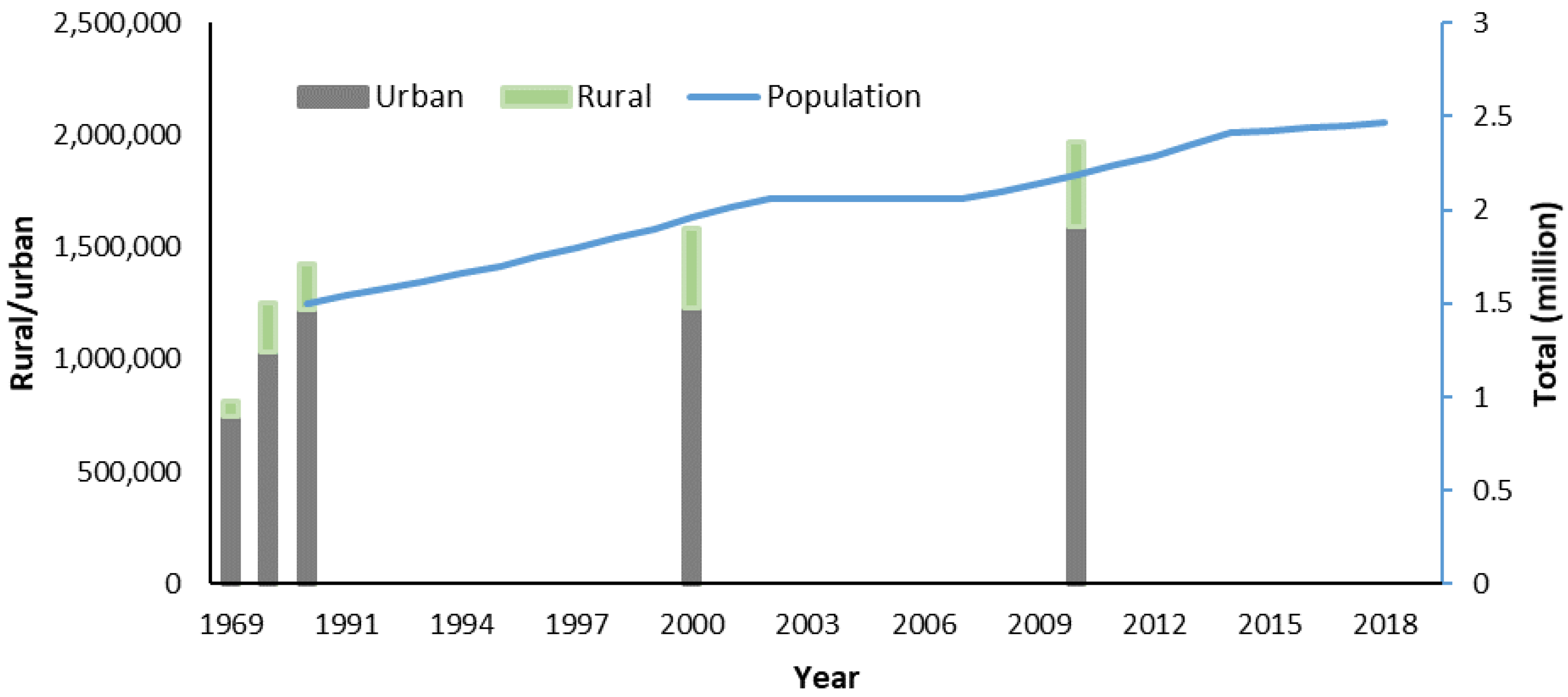
Study Area
2. Materials and Methods
2.1. Time Series Data and Indicators
2.1.1. MODIS (MODerate Resolution Imaging Spectroradiometer)
2.1.2. Parameter Derivation and Trend Estimation
2.2. Additional Data
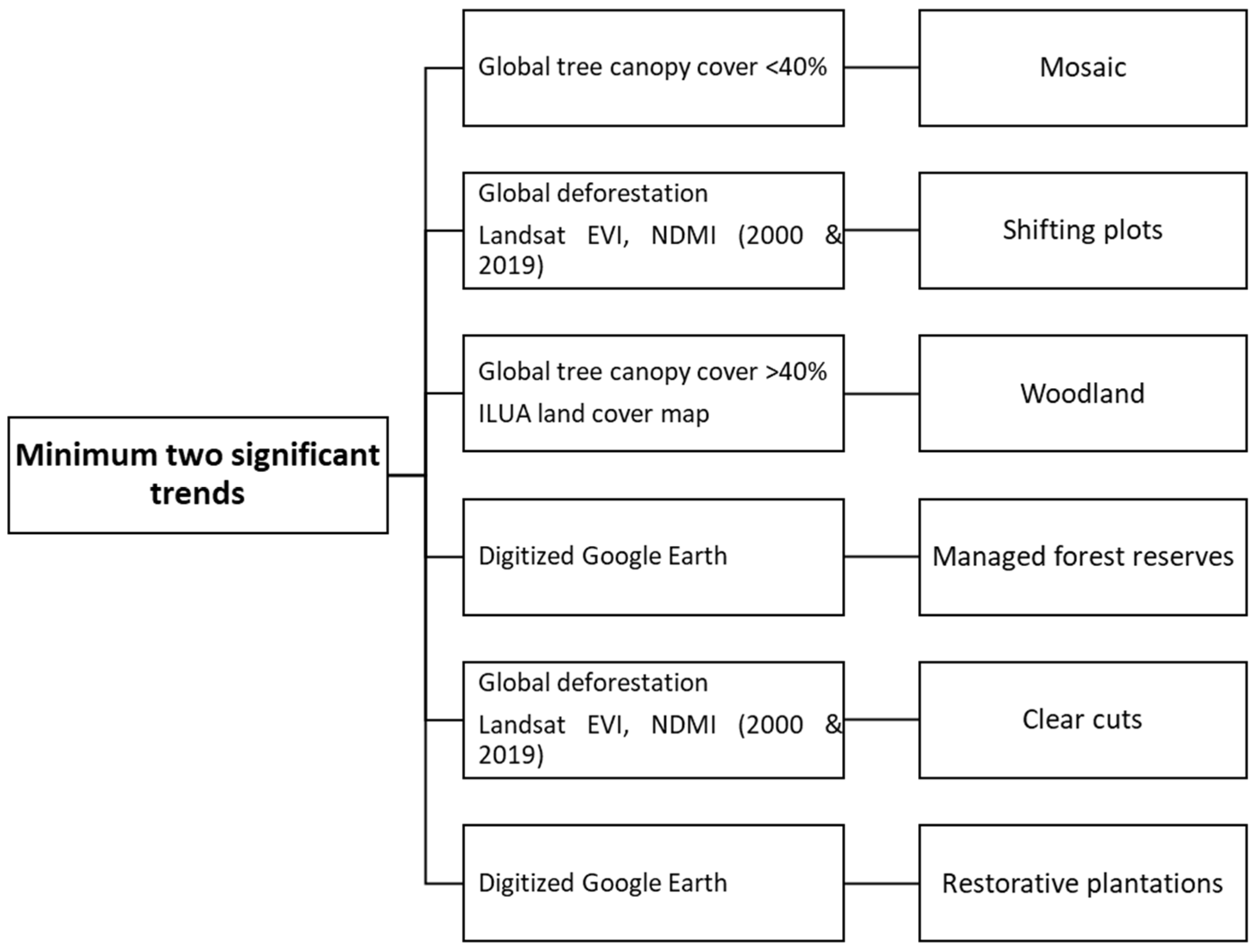
2.3. Assigning Land Change Processes
3. Results
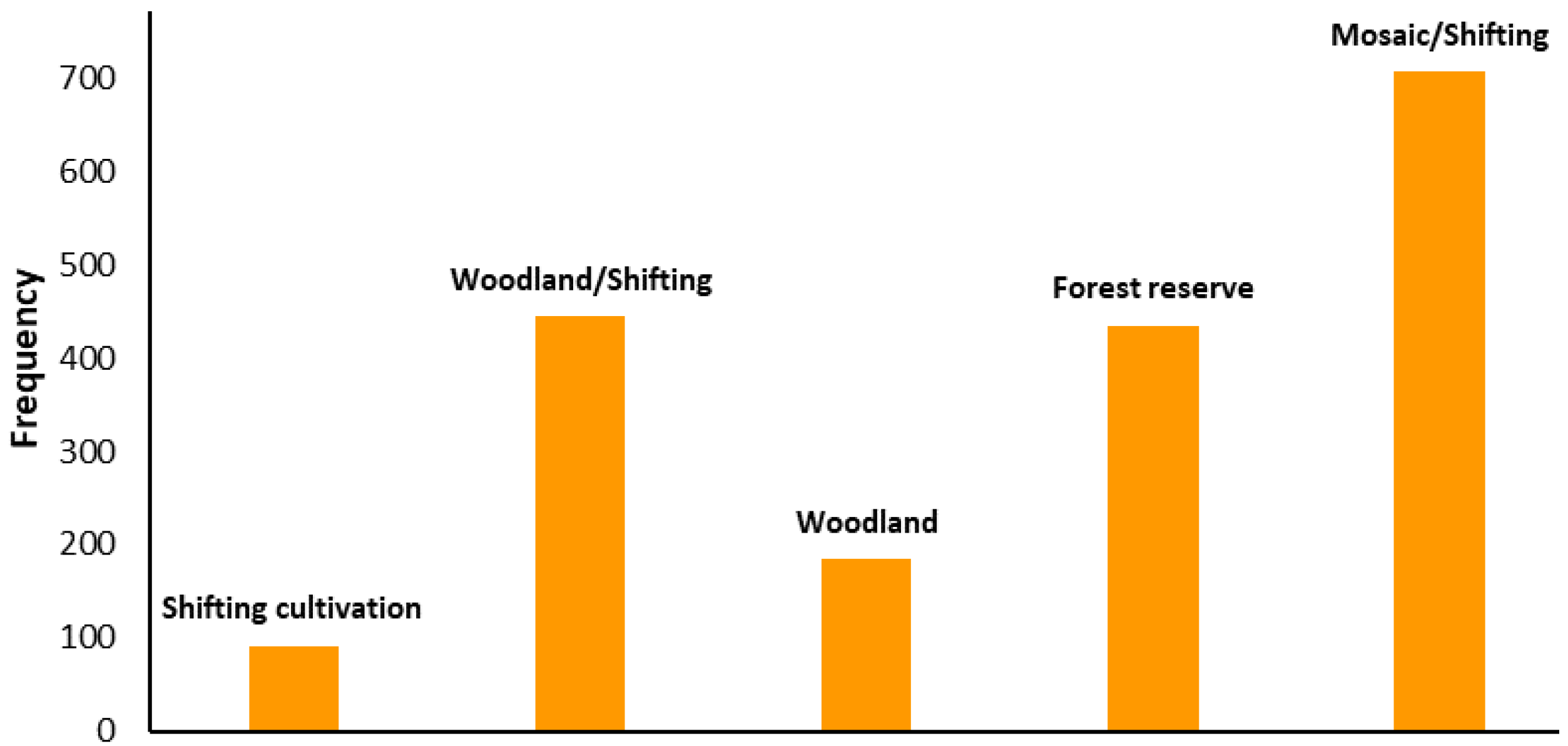
3.1. Trend Analysis
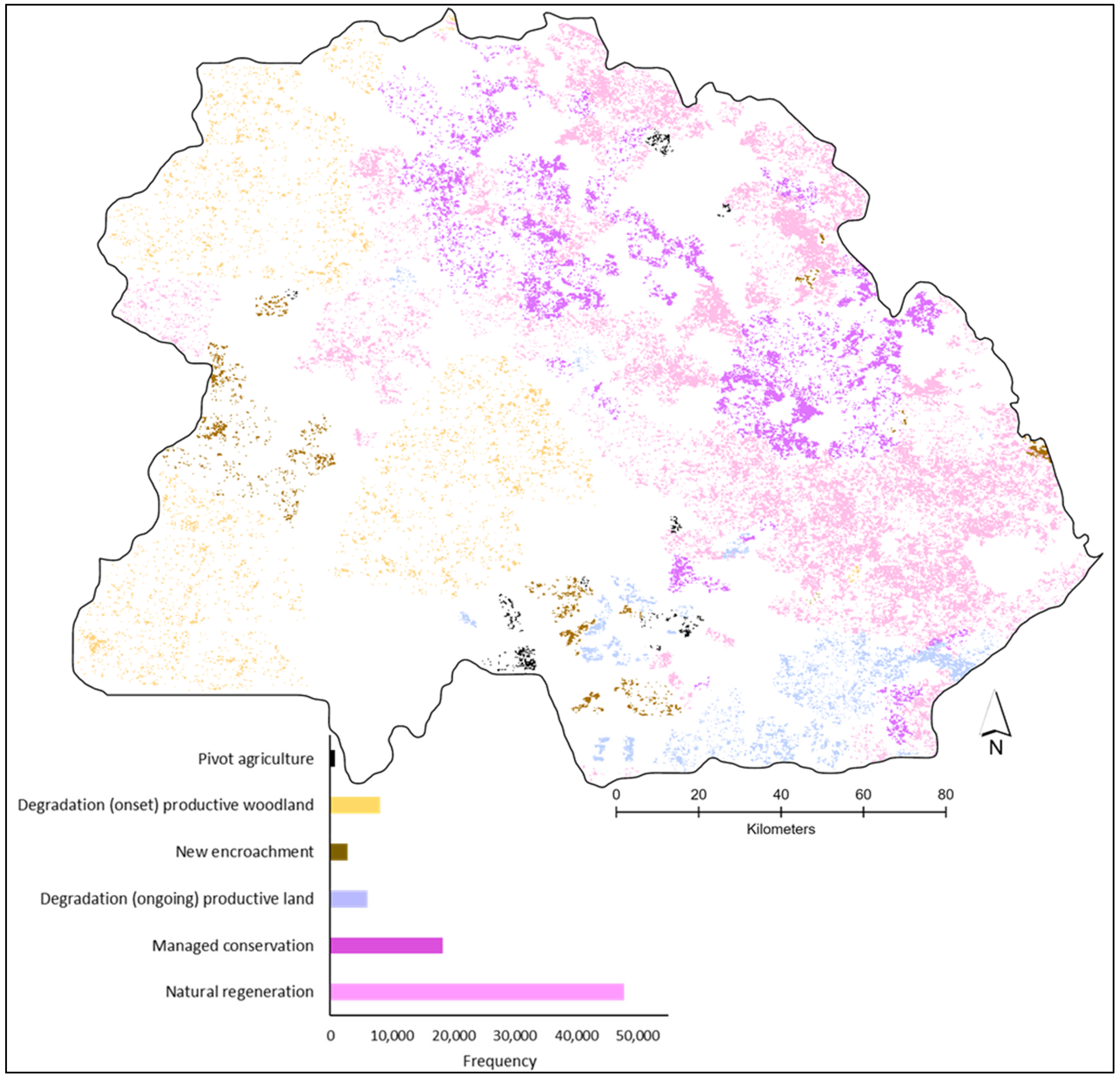
3.2. Land Change Dynamics
4. Discussion
4.1. Degradation
4.2. Recovery
4.3. Land Management
5. Conclusions
Author Contributions
Funding
Data Availability Statement
Acknowledgments
Conflicts of Interest
References
- Vogt, J.V.; Safriel, U.; von Maltitz, G.; Sokona, Y.; Zougmore, R.; Bastin, G.; Hill, J. Monitoring and Assessment of Land Degradation and Desertification: Towards New Conceptual and Integrated Approaches. Land Degrad. Dev. 2011, 22, 150–165. [Google Scholar] [CrossRef]
- Reynolds, J.F.; Maestre, F.T.; Kemp, P.R.; Stafford-Smith, D.M.; Lambin, E. Natural and Human Dimensions of Land Degradation in Drylands: Causes and Consequences. In Terrestrial Ecosystems in a Changing World; Springer: Berlin, Germany, 2007; pp. 247–257. [Google Scholar]
- International Food Policy Research Institute. Global Food Policy Report; International Food Policy Research Institute: Washington, DC, USA, 2013. [Google Scholar]
- Adeel, Z. Ecosystems and Human Well-Being: Desertification Synthesis: A Report of the Millennium Ecosystem Assessment; World Resources Institute: Washington, DC, USA, 2005. [Google Scholar]
- Geist, H.J.; Lambin, E.F. Dynamic Causal Patterns of Desertification. Bioscience 2004, 54, 817–829. [Google Scholar] [CrossRef] [Green Version]
- Schultz, M.; Shapiro, A.; Clevers, J.G.P.W.; Beech, C.; Herold, M. Forest Cover and Vegetation Degradation Detection in the Kavango Zambezi Transfrontier Conservation Area Using BFAST Monitor. Remote Sens. 2018, 10, 1850. [Google Scholar] [CrossRef] [Green Version]
- Veron, S.R.; Paruelo, J.M.; Oesterheld, M. Assessing Desertification. J. Arid. Environ. 2006, 66, 751–763. [Google Scholar] [CrossRef]
- Syampungani, S.; Chirwa, P.W.; Akinnifesi, F.K.; Ajayi, O.C. The Potential of Using Agroforestry as a Win-Win Solution to Climate Change Mitigation and Adaptation and Meeting Food Security Challenges in Southern Africa. Agric. J. 2010, 5, 80–88. [Google Scholar] [CrossRef] [Green Version]
- Munyati, C. Wetland Change Detection on the Kafue Flats, Zambia, by Classification of a Multitemporal Remote Sensing Image Dataset. Int. J. Remote Sens. 2000, 21, 1787–1806. [Google Scholar] [CrossRef]
- Petit, C.; Scudder, T.; Lambin, E. Quantifying Processes of Land-Cover Change by Remote Sensing: Resettlement and Rapid Land-Cover Changes in South-Eastern Zambia. Int. J. Remote Sens. 2001, 22, 3435–3456. [Google Scholar] [CrossRef]
- Simwanda, M.; Murayama, Y. Integrating Geospatial Techniques for Urban Land Use Classification in the Developing Sub-Saharan African City of Lusaka, Zambia. ISPRS Int. J. Geo-Inf. 2017, 6, 102. [Google Scholar] [CrossRef] [Green Version]
- Chomba, B.M.; Tembo, O.; Mutandi, K.; Mtongo, C.S.; Makano, A. Drivers of Deforestation, Identification of Threatened Forests and Forest Co-Benefits Other than Carbon from REDD+ Implementation in Zambia. In A Consultancy Report Prepared for the Forestry Department and the Food and Agriculture Organization of the United Nations under the National UN-REDD Programme; Ministry of Lands, Natural Resources and Environmental Protection: Lusaka, Zambia, 2012. [Google Scholar]
- Mukosha, J.; Siampale, A. Integrated Land Use Assessment (ILUA): Zambia, 2005–2008; Zambia Forestry Department, Ministry of Tourism, Environment and Natural: Lusaka, Zambia, 2008.
- Trapnell, C.G.; Clothier, T.N. The Soils, Vegetation and Agricultural Systems of North-Western Rhodesia; Government Printers: Lusaka, Zambia, 1937.
- Environment Council of Zambia. Zambia Environment Outlook Report 3; Environment Council of Zambia: Lusaka, Zambia, 2008. [Google Scholar]
- Conservation Farming Unit. Conservation Farming in Zambia. Conservation Farming Hand Book for Hoe Farmers in Agro Ecological Region III—The Basics; Conservation Farming Unit: Lusaka, Zambia, 2003. [Google Scholar]
- Mason-Case, S. Legal Preparedness for REDD+ in Zambia: Country Study. In Report Prepared by the International Development Law Organisation (IDLO) with Support from the Food and Agriculture Organisation of the United Nations (FAO) and the UN-REDD Programme; International Development Law Organisation: Rome, Italy, 2011. [Google Scholar]
- Vinya, R.; Syampungani, S.; Kasumu, E.C.; Monde, C.; Kasubika, R. Preliminary Study on the Drivers of Deforestation and Potential for REDD+ in Zambia; FAO/Zambian Ministry of Lands and Natural Resources: Lusaka, Zambia, 2011.
- Oksanen, T.; Mersmann, C. Forests in Poverty Reduction Strategies: An Assessment of PRSP Processes in Sub-Saharan Africa. For. Poverty Reduct. Strateg. Capturing Potential EFI Proc. 2003, 47, 121–158. [Google Scholar]
- Chapoto, A.; Zulu-Mbata, O.; Beaver, M.; Chisanga, B.; Kabwe, S.; Kuteya, A.N.; Munsaka, E.; Namonje-Kapembwa, T.; Tembo, S.; Sitko, N. Rural Agricultural Livelihoods Survey: 2015 Survey Report; Indaba Agricultural Policy Research Institute (IAPRI): Lusaka, Zambia, 2016. [Google Scholar]
- Henry, M.; Maniatis, D.; Gitz, V.; Huberman, D.; Valentini, R. Implementation of REDD+ in Sub-Saharan Africa: State of Knowledge, Challenges and Opportunities. Environ. Dev. Econ. 2011, 16, 381–404. [Google Scholar] [CrossRef] [Green Version]
- Ministry of Tourism, Environment and Natural Resources. Zambia National Action Program for Combating Desertification and Mitigating Serious Effects of Drought; Ministry of Tourism, Environment and Natural Resources: Lusaka, Zambia, 2002.
- Chidumayo, E.N. Development of Reference Emission Levels for Zambia. In Report Prepared for the UN Food and Agriculture Organisation (FAO) and UN Reducing Emissions from Deforestation and Forest Degradation (UN REDD); Makeni Savanna Research Project: Lusaka, Zambia, 2012. [Google Scholar]
- Kalaba, F.K. Barriers to Policy Implementation and Implications for Zambia’s Forest Ecosystems. For. Policy Econ. 2016, 69, 40–44. [Google Scholar] [CrossRef]
- Tucker, C.J. Red and Photographic Infrared Linear Combinations for Monitoring Vegetation. Remote Sens. Environ. 1979, 8, 127–150. [Google Scholar] [CrossRef] [Green Version]
- Graetz, R.D. Empirical and Practical Approaches to Land Surface Characterisation and Change Detection. In The Use of Remote Sensing for Land Degradation and Desertification Monitoring in the Mediterranean Basin; European Commission: Brussels, Belgium, 1996; pp. 9–22. [Google Scholar]
- Hill, J.; Hostert, P.; Röder, A. Long-Term Observation of Mediterranean Ecosystems with Satellite Remote Sensing. In Recent Dynamics of the Mediterranean Vegetation and Landscape; John Wiley & Sons Ltd: Chichester, UK, 2004; pp. 33–43. [Google Scholar]
- Gobron, N.; Verstraete, M.M.; Pinty, B.; Taberner, M.; Aussedat, O. Potential of Long Time Series of FAPAR Products for Assessing and Monitoring Land Surface Changes: Examples in Europe and the Sahel. In Recent Advances in Remote Sensing and Geoinformation Processing for Land Degradation Assessment; CRC Press: London, UK, 2009; pp. 109–122. ISBN 042920681X. [Google Scholar]
- Cho, M.A.; Ramoelo, A. Optimal Dates for Assessing Long-Term Changes in Tree-Cover in the Semi-Arid Biomes of South Africa Using MODIS NDVI Time Series (2001–2018). Int. J. Appl. Earth Obs. Geoinf. 2019, 81, 27–36. [Google Scholar] [CrossRef]
- Leroux, L.; Bégué, A.; Seen, D.L.; Jolivot, A.; Kayitakire, F. Driving Forces of Recent Vegetation Changes in the Sahel: Lessons Learned from Regional and Local Level Analyses. Remote Sens. Environ. 2017, 191, 38–54. [Google Scholar] [CrossRef] [Green Version]
- Schneibel, A.; Stellmes, M.; Röder, A.; Frantz, D.; Kowalski, B.; Haß, E.; Hill, J. Assessment of Spatio-Temporal Changes of Smallholder Cultivation Patterns in the Angolan Miombo Belt Using Segmentation of Landsat Time Series. Remote Sens. Environ. 2017, 195, 118–129. [Google Scholar] [CrossRef] [Green Version]
- Phiri, D.; Morgenroth, J.; Xu, C. Long-Term Land Cover Change in Zambia: An Assessment of Driving Factors. Sci. Total Environ. 2019, 697, 134206. [Google Scholar] [CrossRef]
- Fiorillo, E.; Maselli, F.; Tarchiani, V.; Vignaroli, P. Analysis of Land Degradation Processes on a Tiger Bush Plateau in South West Niger Using MODIS and LANDSAT TM/ETM+ Data. Int. J. Appl. Earth Obs. Geoinf. 2017, 62, 56–68. [Google Scholar] [CrossRef]
- Higginbottom, T.P.; Symeonakis, E. Identifying Ecosystem Function Shifts in Africa Using Breakpoint Analysis of Long-Term NDVI and RUE Data. Remote Sens. 2020, 12, 1894. [Google Scholar] [CrossRef]
- Zimba, H.; Kawawa, B.; Chabala, A.; Phiri, W.; Selsam, P.; Meinhardt, M.; Nyambe, I. Assessment of Trends in Inundation Extent in the Barotse Floodplain, Upper Zambezi River Basin: A Remote Sensing-Based Approach. J. Hydrol. Reg. Stud. 2018, 15, 149–170. [Google Scholar] [CrossRef]
- Munawar, S.; Udelhoven, T. Land Change Syndromes Identification in Temperate Forests of Hindukush Himalaya Karakorum (HHK) Mountain Ranges. Int. J. Remote Sens. 2020, 41, 7735–7756. [Google Scholar] [CrossRef]
- Huete, A.; Didan, K.; Miura, T.; Rodriguez, E.P.; Gao, X.; Ferreira, L.G. Overview of the Radiometric and Biophysical Performance of the MODIS Vegetation Indices. Remote Sens. Environ. 2002, 83, 195–213. [Google Scholar] [CrossRef]
- Team, A. Application for Extracting and Exploring Analysis Ready Samples (AppEEARS); Version 2.49; NASA EOSDIS Land Processes Distributed Active Archive Center (LP DAAC), USGS/Earth Resources Observation and Science (EROS) Center: Sioux Falls, SD, USA, 2020. [Google Scholar]
- Atzberger, C.; Eilers, P.H.C. A Time Series for Monitoring Vegetation Activity and Phenology at 10-Daily Time Steps Covering Large Parts of South America. Int. J. Digit. Earth 2011, 4, 365–386. [Google Scholar] [CrossRef]
- Mattiuzzi, M.; Lobo, A. Acquisition and Processing of MODIS Products; R Package: Vienna, Austria, 2012. [Google Scholar]
- Ollinger, S.V. Sources of Variability in Canopy Reflectance and the Convergent Properties of Plants. New Phytol. 2011, 189, 375–394. [Google Scholar] [CrossRef]
- Verbesselt, J.; Hyndman, R.; Zeileis, A.; Culvenor, D. Phenological Change Detection While Accounting for Abrupt and Gradual Trends in Satellite Image Time Series. Remote Sens. Environ. 2010, 114, 2970–2980. [Google Scholar] [CrossRef] [Green Version]
- Tateishi, R.; Ebata, M. Analysis of Phenological Change Patterns Using 1982–2000 Advanced Very High Resolution Radiometer (AVHRR) Data. Int. J. Remote Sens. 2004, 25, 2287–2300. [Google Scholar] [CrossRef]
- Zeileis, A.; Kleiber, C.; Krämer, W.; Hornik, K. Testing and Dating of Structural Changes in Practice. Comput. Stat. Data Anal. 2003, 44, 109–123. [Google Scholar] [CrossRef] [Green Version]
- R Core TEAM. R: A Language and Environment for Statistical Computing; R Foundation for Statistical Computing: Vienna, Austria, 2009. [Google Scholar]
- Forkel, M.; Carvalhais, N.; Verbesselt, J.; Mahecha, M.D.; Neigh, C.S.R.; Reichstein, M. Trend Change Detection in NDVI Time Series: Effects of Inter-Annual Variability and Methodology. Remote Sens. 2013, 5, 2113–2144. [Google Scholar] [CrossRef] [Green Version]
- Hansen, M.C.; Potapov, P.V.; Moore, R.; Hancher, M.; Turubanova, S.A.; Tyukavina, A.; Thau, D.; Stehman, S.V.; Goetz, S.J.; Loveland, T.R. High-Resolution Global Maps of 21st-Century Forest Cover Change. Science 2013, 342, 850–853. [Google Scholar] [CrossRef] [Green Version]
- OpenStreetMap contributors Copyright and License. Available online: https://www.openstreetmap.org/copyright (accessed on 3 January 2022).
- Ives, A.R.; Zhu, L.; Wang, F.; Zhu, J.; Morrow, C.J.; Radeloff, V.C. Statistical Inference for Trends in Spatiotemporal Data. Remote Sens. Environ. 2021, 266, 112678. [Google Scholar] [CrossRef]
- Mayr, S.; Kuenzer, C.; Gessner, U.; Klein, I.; Rutzinger, M. Validation of Earth Observation Time-Series: A Review for Large-Area and Temporally Dense Land Surface Products. Remote Sens. 2019, 11, 2616. [Google Scholar] [CrossRef] [Green Version]
- Copperbelt Provincial Administration Agriculture Investment Opportunities. Available online: https://www.cbt.gov.zm/?page_id=4539 (accessed on 9 December 2021).
- Kwesiga, F.; Franzel, S.; Matongoya, P.; Ajayi, O.; Phiri, D.; Katanga, R.; Kuntashula, E.; Place, F.; Chira, T. Improved Fallows in Eastern Zambia: History, Farmer Practice and Impacts; Successes in African Agriculture Conference Background Paper No.12 and Environment and Production Technology Division Working Paper, 108; International Food Policy Research Institute: Washington, DC, USA, 2003. [Google Scholar]
- Zambia Forestry Action Plan. Zambia Forestry Action Plan 1997–2015; Ministry of Environment and Natural Resoucres, Ed.; Forestry Department: Lusaka, Zambia, 1997.
- Mulenga, B.; Nkonde, C.; Ngoma, H. Does Customary Land Tenure System Encourage Local Forestry Management in Zambia? A Focus on Wood Fuel; Indaba Agricultural Policy Research Institute: Lusaka, Zambia, 2015. [Google Scholar]
- Kazungu, M.; Zhunusova, E.; Yang, A.L.; Kabwe, G.; Gumbo, D.J.; Günter, S. Forest Use Strategies and Their Determinants among Rural Households in the Miombo Woodlands of the Copperbelt Province, Zambia. For. Policy Econ. 2020, 111, 102078. [Google Scholar] [CrossRef]
- Handavu, F.; Chirwa, P.W.C.; Syampungani, S. Socio-Economic Factors Influencing Land-Use and Land-Cover Changes in the Miombo Woodlands of the Copperbelt Province in Zambia. For. Policy Econ. 2019, 100, 75–94. [Google Scholar] [CrossRef] [Green Version]
- Chidumayo, E. Charcoal Potential in Southern Africa (CHAPOSA): Final Report for Zambia; Stockholm Environment Institute: Lusaka, Zambia, 2002. [Google Scholar]
- Dlamini, C.; Moombe, B.; Syampungani, S.; Samboko, P.C. Load Shedding and Charcoal Use in Zambia: What Are the Implications on Forest Resources. In Policy Brief; Working Paper 109; Indaba Agricultural Policy Research Institute: Lusaka, Zambia, 2016. [Google Scholar]
- Schneibel, A.; Stellmes, M.; Röder, A.; Finckh, M.; Revermann, R.; Frantz, D.; Hill, J. Evaluating the Trade-off between Food and Timber Resulting from the Conversion of Miombo Forests to Agricultural Land in Angola Using Multi-Temporal Landsat Data. Sci. Total Environ. 2016, 548, 390–401. [Google Scholar] [CrossRef] [PubMed]
- Syampungani, S.; Chirwa, P.W.; Geldenhuys, C.J.; Handavu, F.; Chishaleshale, M.; Rija, A.A.; Mbanze, A.A.; Ribeiro, N.S. Managing Miombo: Ecological and Silvicultural Options for Sustainable Socio-Economic Benefits. In Miombo Woodlands in a Changing Environment: Securing the Resilience and Sustainability of People and Woodlands; Springer: Cham, Switzerland, 2020; pp. 101–137. [Google Scholar]
- Van Wyk, G.F.; Everard, D.A.; Midgley, J.J.; Gordon, I.G. Classification and Dynamics of a Southern African Subtropical Coastal Lowland Forest. South Afr. J. Bot. 1996, 62, 133–142. [Google Scholar] [CrossRef] [Green Version]
- Reader, R.J.; Bricker, B.D. Value of Selectively Cut Deciduous Forest for Understory Herb Conservation: An Experimental Assessment. For. Ecol. Manag. 1992, 51, 317–327. [Google Scholar] [CrossRef]
- Ng’andwe, P. Forest Classification, Zones and Classes—Basis for Industrial Processing; Ministry of Lands, Natural Resources and Environmental Protection, FAO: Lusaka, Zambia, 2012.
- Zambia Forestry and Forest Industries Corporation. Annual Report; Zambia Forestry and Forest Industries Corporation: Ndola, Zambia, 2019. [Google Scholar]
- Ng’andwe, P.; Muima-Kankolongo, A.; Banda, M.K.; Mwitwa, J.P.; Shakacite, O. Forest Revenue, Concession Systems and the Contribution of the Forestry Sector to Poverty Reduction and Zambia’s National Economy. In A Draft Analytical Report Prepared for FAO in Conjunction with the Forestry Department and the Ministry of Tourism, Environment and Natural Resources; Forestry Department and the Ministry of Tourism, Environment and Natural Resources: Lusaka, Zambia, 2006. [Google Scholar]
- Pelletier, J.; Hamalambo, B.; Trainor, A.; Barrett, C.B. How Land Tenure and Labor Relations Mediate Charcoal’s Environmental Footprint in Zambia: Implications for Sustainable Energy Transitions. World Dev. 2021, 146, 105600. [Google Scholar] [CrossRef]


| Original Time Series | Parameters | Derivation |
|---|---|---|
| Bi monthly | Monthly composites | Harmonic model |
| Peaking magnitude | Annual maximum EVI | |
| 1 MGS | Average EVI between 2 SOS and 2 EOS |
| Land Use Type 2000 | Land Use Type 2019 |
|---|---|
| Land use change | |
| Natural woodland | b Shifting plots |
| g Pivot | |
| 1 g Pivot | |
| 1 g Mosaic | |
| Shifting plots | g Pivot |
| g Mosaic | |
| g Restorative plantation | |
| Mosaic | b Shifting plots |
| Similar land use | |
| Natural woodland | b Exploitation |
| g Natural regrowth | |
| m Shifting plots | |
| m Mosaic | |
| Managed forest reserves | b Clear cuts |
| g Conservation | |
| Trend | MGS | Peak | Harmonic |
|---|---|---|---|
| Browning | 3% | 7% | 4% |
| Non-significant (stable) | 70% | 77% | 89% |
| Greening | 27% | 16% | 7% |
| Main Class: Land Change Dynamic | Sub Class |
|---|---|
| Pivot agriculture | 10 Shifting plots to Pivot |
| 12 Pivot | |
| 11 Woodland to Pivot | |
| Degradation (onset) productive woodland | 5 Woodland |
| New encroachment | 8 Woodland to Shifting plots |
| Degradation (ongoing) productive land | 9 Shifting plots |
| 7 Mosaic to Shifting plots | |
| Managed conservation | 3 Forest reserves |
| 6 Shifting plots to Plantations | |
| Natural regeneration | 1 Mosaic |
| 4 Woodland to Mosaic | |
| 2 Shifting plots to Mosaic |
Publisher’s Note: MDPI stays neutral with regard to jurisdictional claims in published maps and institutional affiliations. |
© 2022 by the authors. Licensee MDPI, Basel, Switzerland. This article is an open access article distributed under the terms and conditions of the Creative Commons Attribution (CC BY) license (https://creativecommons.org/licenses/by/4.0/).
Share and Cite
Munawar, S.; Röder, A.; Syampungani, S.; Udelhoven, T. Place-Based Analysis of Satellite Time Series Shows Opposing Land Change Patterns in the Copperbelt Region of Zambia. Forests 2022, 13, 134. https://doi.org/10.3390/f13010134
Munawar S, Röder A, Syampungani S, Udelhoven T. Place-Based Analysis of Satellite Time Series Shows Opposing Land Change Patterns in the Copperbelt Region of Zambia. Forests. 2022; 13(1):134. https://doi.org/10.3390/f13010134
Chicago/Turabian StyleMunawar, Sana, Achim Röder, Stephen Syampungani, and Thomas Udelhoven. 2022. "Place-Based Analysis of Satellite Time Series Shows Opposing Land Change Patterns in the Copperbelt Region of Zambia" Forests 13, no. 1: 134. https://doi.org/10.3390/f13010134